ESTIMATION OF LARGE COVARIANCE AND PRECISION MATRICES FROM TEMPORALLY DEPENDENT OBSERVATIONS

Abstract

We consider the estimation of large covariance and precision matrices from high-dimensional sub-Gaussian or heavier-tailed observations with slowly decaying temporal dependence. The temporal dependence is allowed to be long-range so with longer memory than those considered in the current literature. We show that several commonly used methods for independent observations can be applied to the temporally dependent data. In particular, the rates of convergence are obtained for the generalized thresholding estimation of covariance and correlation matrices, and for the constrained $\ell_{1}$ minimization and the $\ell_{1}$ penalized likelihood estimation of precision matrix. Properties of sparsistency and sign-consistency are also established. A gap-block cross-validation method is proposed for the tuning parameter selection, which performs well in simulations. As a motivating example, we study the brain functional connectivity using resting-state fMRI time series data with long-range temporal dependence.

and

t1Supported in part by NIH grant R01-AG036802 and NSF grant DMS-1407142.

1 Introduction

Let $\{\boldsymbol{X}_{1},\dots,\boldsymbol{X}_{n}\}$ be a sample of $p$-dimensional random vectors, each with the same mean $\boldsymbol{\mu}_{p}$, covariance matrix $\mathbf{\Sigma}$ and precision matrix $\mathbf{\Omega}=\mathbf{\Sigma}^{-1}$. It is well known that the sample covariance matrix is not a consistent estimator of $\mathbf{\Sigma}$ when $p$ grows with $n$ [3, 4]. When the sample observations $\boldsymbol{X}_{1},\dots,\boldsymbol{X}_{n}$ are independent and identically distributed (i.i.d.), several regularization methods have been proposed for the consistent estimation of large $\mathbf{\Sigma}$, including thresholding [10, 18, 32, 63], block-thresholding [21], banding [11] and tapering [22]. Existing methods also include Cholesky-based method [48, 64], penalized pseudo-likelihood method [50] and sparse matrix transform [24]. Consistent correlation matrix estimation can be obtained similarly from i.i.d. observations [32, 49].

The precision matrix $\mathbf{\Omega}=(\omega_{ij})_{p\times p}$, when it exists, is closely related to the partial correlations between the pairs of variables in a vector $\boldsymbol{X}$. Specifically, the partial correlation between $X_{i}$ and $X_{j}$ given $\{X_{k},k\neq i,j\}$ is equal to $-\omega_{ij}/\sqrt{\omega_{ii}\omega_{jj}}$ [30]. Zero partial correlation means conditional independence between Gaussian or nonparanormal random variables [53]. There is a rich literature on the estimation of large $\mathbf{\Omega}$ from i.i.d. observations. Various algorithms for the $\ell_{1}$ penalized maximum likelihood method ($\ell_{1}$-MLE) and its variants have been developed [5, 37, 46, 78], and related theoretical properties have been investigated by [50, 61, 62]. Methods of estimating $\mathbf{\Omega}$ column-by-column thus implementable with parallel computing include nodewise Lasso [56, 71], graphical Dantzig selector [77], constrained $\ell_{1}$-minimization for inverse matrix estimation (CLIME) [19], and adaptive CLIME [20].

Recently, researchers become increasingly interested in estimating the large covariance and precision matrices from temporally dependent observations $\{\boldsymbol{X}_{t}:t=1,\dots,n\}$, here $t$ denotes time. Such research is particularly useful in analyzing the resting-state functional magnetic resonance imaging (rfMRI) data to assess the brain functional connectivity [58, 66]. In such imaging studies, the number of brain nodes (voxels or regions of interest) $p$ can be greater than the number of images $n$. The temporal dependence of time series $\boldsymbol{X}_{t}$ is traditionally dealt with by imposing the so-called strong mixing conditions [14]. To overcome the difficulties in computing strong mixing coefficients and verifying strong mixing conditions, [74] introduced a new type of dependence measure, the functional dependence measure, and recently applied it to the hard thresholding estimation of large covariance matrix and the $\ell_{1}$-MLE type methods of large precision matrix [25]. The functional dependence measure may still be difficult to understand and to interpret for most data analysts. Practically, it is straightforward to describe the temporal dependence directly by using cross-correlations [15]. By imposing certain weak dependence conditions on the cross-correlation matrix of samples $\{\boldsymbol{X}_{t}\}_{t=1}^{n}$, [8, 9] extended the banding and tapering regularization methods for estimating covariance matrix.

A univariate stationary time series is said to be long-memory if its autocorrelation function $\rho(t)$ satisfies $\sum_{t=0}^{\infty}|\rho(t)|=\infty$, and short-memory otherwise [57]. The rfMRI data have been reported with long-memory in the scientific literature, e.g., [43, 69]. However, the temporal dependence considered by [25] and that considered by [8, 9] do not cover any long-memory time series. Later we will illustrate that the rfMRI data example does not meet their restrictive temporal dependence conditions. Hence, it is important to show the applicability of the estimating methods for i.i.d. samples to this kind of data. In this article, we propose a new and straightforward temporal dependence measure that solely depends on the Frobenius norm and the spectral norm of the autocorrelation matrices of $\{\boldsymbol{X}_{t}\}_{t=1}^{n}$. Such a new measure clearly displays the effect of temporal dependence on the convergence rates of our considered matrix estimators, allowing each time series to be long-memory or even to be non-stationary. So the rfMRI data can be well handled by our relaxed assumption (see Figure 1). To the best of our knowledge, this is the first work that investigates the estimation of large covariance and precision matrices from long-memory observations.

Note that the estimation of large correlation matrix was not considered by either [25] or [8, 9], which is a more interesting problem in, for example, the study of brain functional connectivity. It was considered in a recent work by [80] but under the assumption that all $p$ time series have the same temporal decay rate, which is rather restrictive and often violated (see Figure 1 for an example of rfMRI data). Moreover, all four aforementioned articles assumed that $\boldsymbol{\mu}_{p}=(\mu_{pi})_{1\leq i\leq p}$ is known, which may not be true in practice. Although the sample mean $\bar{X}_{i}=\frac{1}{n}\sum_{j=1}^{n}X_{ij}$ entrywise converges to $\mu_{pi}$ in probability or even almost surely under some dependence conditions [15, 47], extra care will still be needed when true mean is replaced by sample mean in the matrix estimation, especially for long-memory, heavy-tailed, or even non-stationary data. We consider unknown $\boldsymbol{\mu}_{p}$ in this article, and show that the mean estimation indeed affects our derived matrix convergence rates, particularly for data with heavy tail probabilities.

In this article, we study the generalized thresholding estimation [63] for covariance and correlation matrices, and the CLIME approach [19] and an $\ell_{1}$-MLE type method called sparse permutation invariant covariance estimation (SPICE; [62]) for precision matrix. The convergence rates, sparsistency and sign-consistency are provided for temporally dependent data, potentially with long memory, which are generated from a linear spatio-temporal model with all basis random variables coming from sub-Gaussian, or generalized sub-exponential, or distributions with polynomial-type tails. We also establish the minimax optimal convergence rates of estimating covariance and correlation matrices for a certain class of temporally dependent sub-Gaussian data, including short-memory and some long-memory cases, and show that they can be achieved by the generalized thresholding method. Moreover, if the matrix $\ell_{1}$ norm of the precision matrix is bounded by a constant for such data, then the CLIME estimator attains the minimax optimal rates for i.i.d. observations shown in [20].

The article is organized as follows. In Section 2, we introduce the new temporal dependence measure and the considered temporally dependent data generating mechanism. We provide the theoretical results for the estimation of covariance and correlation matrices in Section 3 and for the estimation of precision matrix in Section 4 for temporally dependent observations with sub-Gaussian tails. We consider extensions to data with generalized sub-exponential tails and polynomial-type tails in Section 5. In Section 6, we introduce a gap-block cross-validation method for the tuning parameter selection, evaluate the estimating performance via simulations, and analyze a rfMRI data set for brain functional connectivity. The concentration inequalities that the proofs of the theoretical results are based on are given in the Appendix. Detailed proofs together with additional numerical considerations are provided in the Supplementary Material due to the page limitation.

2 Temporal dependence

We start with a brief introduction of useful notation. For a real matrix $\mathbf{M}=(M_{ij})$, we define: the spectral norm $\|\mathbf{M}\|_{2}=[\varphi_{\max}{(\mathbf{M}^{\top}\mathbf{M})}]^{1/2}$, where $\varphi_{\max}$ is the largest eigenvalue, also $\varphi_{k}$ and $\varphi_{\min}$ are the $k$-th and the smallest eigenvalues, respectively; the Frobenius norm $\|\mathbf{M}\|_{F}=(\sum_{i}\sum_{j}M_{ij}^{2})^{1/2}$; the matrix $\ell_{1}$ norm $\|\mathbf{M}\|_{1}=\max_{j}\sum_{i}|M_{ij}|$; the entrywise $\ell_{1}$ norm $|\mathbf{M}|_{1}=\sum_{i,j}|M_{ij}|$ and its off-diagonal version $|\mathbf{M}|_{1,\text{off}}=\sum_{i\neq j}|M_{ij}|$; and the entrywise $\ell_{\infty}$ norm $|\mathbf{M}|_{\infty}=\max_{i,j}|M_{ij}|$.

Denote $\textup{vec}(\mathbf{M})$ $=(\boldsymbol{M}_{1}^{\top},\dots,\boldsymbol{M}_{n}^{\top})^{\top}$, where $\boldsymbol{M}_{j}$ is the $j$-th column of $\mathbf{M}$. Write $\mathbf{M}\succ 0$ when $\mathbf{M}$ is positive definite. Denote the trace and the determinant of a square matrix $\mathbf{M}$ by $\text{tr}(\mathbf{M})$ and $\text{det}(\mathbf{M})$, respectively. Denote the Kronecker product by $\otimes$. Write $x_{n}\asymp y_{n}$ if $x_{n}=O(y_{n})$ and $y_{n}=O(x_{n})$, and denote $x_{n}\sim y_{n}$ if $x_{n}/y_{n}\to 1$ as $n\to\infty$. Define $\lceil{x}\rceil$ and $\lfloor{x}\rfloor$ to be the smallest integer $\geq x$ and the largest integer $\leq x$, respectively. Let $\mathds{1}(A)$ be the indicator function of event $A$, $x_{+}=x\mathds{1}(x\geq 0)$ and sign$(x)=\mathds{1}(x\geq 0)-\mathds{1}(x\leq 0)$. Let $A\coloneqq B$ denote that $A$ is defined to be $B$. Denote $X\stackrel{{\scriptstyle d}}{{=}}Y$ if $X$ and $Y$ have the same distribution. Denote $\boldsymbol{1}_{n}=(1,1,\dots,1)^{\top}$ with length $n$ and $\mathbf{I}_{n\times n}$ to be the $n{\times}n$ identity matrix. If without further notification, a constant is independent of $n$ and $p$. Throughout the rest of the article, we assume $p\to\infty$ as $n\to\infty$ and only use $n\to\infty$ in the asymptotic arguments.

2.1 A new temporal dependence measure

Let $\mathbf{X}_{p\times n}\coloneqq(\boldsymbol{X}_{1},...,\boldsymbol{X}_{n})$, where each column $\boldsymbol{X}_{i}$ follows a distribution with the same covariance matrix $\mathbf{\Sigma}=({\sigma}_{k\ell})_{p\times p}$ and correlation matrix $\mathbf{R}=(\rho_{k\ell})_{p\times p}$. Let $\boldsymbol{X}_{[1]},\dots,\boldsymbol{X}_{[p]}$ be the $p$ row vectors of $\mathbf{X}_{p\times n}$, and $\mathbf{R}_{[k]}=(\rho_{[k]}^{ij})_{n\times n}$ be the correlation matrix of $\boldsymbol{X}_{[k]}$, i.e., the autocorrelation matrix of the $k$-th time series. For all $k$, we have the following inequalities:

$$1\leq\frac{1}{n}\|\mathbf{R}_{[k]}\|_{F}^{2}\leq\|\mathbf{R}_{[k]}\|_{2}\leq\|\mathbf{R}_{[k]}\|_{1}\leq n,$$ (1)

where the second inequality follows from

$$\frac{1}{n}\text{tr}(\mathbf{R}_{[k]}^{2})=\frac{1}{n}\sum_{i=1}^{n}\varphi_{i}^{2}(\mathbf{R}_{[k]})\leq\frac{1}{n}\varphi_{\max}(\mathbf{R}_{[k]})\sum_{i=1}^{n}\varphi_{i}(\mathbf{R}_{[k]})=\frac{1}{n}\|\mathbf{R}_{[k]}\|_{2}\text{tr}(\mathbf{R}_{[k]}),$$

and the third inequality is obtained from Corollary 2.3.2 in [39].

Define a joint temporal dependence measure that consists of two components bounded by $g_{F}$ and $g_{2}$, respectively:

$$\max_{1\leq k\leq p}\frac{1}{n}\|\mathbf{R}_{[k]}\|_{F}^{2}\leq g_{F},\ \max_{1\leq k\leq p}\|\mathbf{R}_{[k]}\|_{2}\leq g_{2},$$ (2)

and from (1) we set $1\leq g_{F}\leq g_{2}\leq n$. The proposed measure naturally describes the overall strength of temporal dependence of the $p$ time series. Particularly, we can set $g_{2}=1$ if all the $p$ time series are white noise processes, and $g_{F}=n$ if every pair of data points in one of the time series are perfectly correlated or anti-correlated.

Later we will show that the convergence rates of considered estimators are nicely characterized by the bounds $g_{F}$ and $g_{2}$, which is particularly useful in obtaining convergence results for long-memory data. Note that we do not consider cross-correlations between the multiple time series, neither assume any specific temporal decay model or stationarity for autocorrelations within each individual time series. Here are two special examples of practical interests.

Case 1 (High-dimensional short-memory dependence).

Recall that a univariate stationary time series is said to be short-memory if its autocorrelation function satisfies $\sum_{t=0}^{\infty}|\rho(t)|<\infty$. We extend the “short-memory” concept to multivariate time series that are allowed to be non-stationary by the property

$$\max_{1\leq k\leq p}\|\mathbf{R}_{[k]}\|_{1}<\infty\ \text{as}\ n\to\infty.$$ (3)

Thus from (1) we can set the measure bound $g_{2}<\infty$ as $n\to\infty$.

Case 2 (Polynomial-dominated decay (PDD) model).

We say $\mathbf{X}_{p\times n}$ has PDD temporal dependence if

$$\max_{1\leq k\leq p}\big{|}\rho_{[k]}^{ij}\big{|}\leq C_{0}|i-j|^{-\alpha}\quad\text{for all $i\neq j$}$$ (4)

with some positive constants $C_{0}$ and $\alpha$. We can then set the measure bounds

$$g_{F}=2C_{0}^{2}H_{\lceil{n/2}\rceil}^{(2\alpha)}+1\quad\text{and}\quad g_{2}=2C_{0}H_{\lceil{n/2}\rceil}^{(\alpha)}+1\geq\max_{1\leq k\leq p}\|\mathbf{R}_{[k]}\|_{1}$$ (5)

with the generalized harmonic number (see (25), (26) in [27])

$$H_{n}^{(\alpha)}=\sum_{k=1}^{n}k^{-\alpha}<1+\begin{cases}\frac{n^{1-\alpha}-1}{1-\alpha},&\alpha\neq 1;\\ \log n,&\alpha=1.\end{cases}$$ (6)

The model is short-memory in the sense of (3) when $\alpha>1$, but allows an individual time series to be long-memory when $0<\alpha\leq 1$. It is worth noting that the fractional Gaussian noise [54, 70] and the autoregressive fractionally integrated moving average process [40, 45] are classical examples of stationary univariate time series with autocorrelation function $\rho(t)\sim Ct^{-\alpha}$ as $t\to\infty$ with $C\neq 0$ and $\alpha\in(0,1)\cup(1,2)$.

2.2 Comparisons to existing work

For banding and tapering estimators of $\mathbf{\Sigma}$, [8] considered a weak temporal dependence $\max_{a_{n}\leq|i-j|\leq n}{|\mathbf{\Lambda}^{ij}|_{\infty}}=$ $O(n^{-2}a_{n}),$ where $\mathbf{\Lambda}^{ij}=(\varLambda_{k\ell}^{ij})_{p\times p}$ with $\varLambda_{k\ell}^{ij}$ satisfying $\textup{Cov}(X_{ki},X_{\ell j})=\varLambda_{k\ell}^{ij}\sigma_{k\ell}$, $a_{n}\sqrt{\log p/n}=o(1)$, and $\{a_{n}\}_{n\geq 1}$ is a non-decreasing sequence of non-negative integers. That $a_{n}\sqrt{\log p/n}=o(1)$ implies $a_{n}=o(\sqrt{n})$. Thus, $\left|\mathbf{\Lambda}^{ij}{:}|i-j|{=}\lfloor\sqrt{n}\rfloor\right|_{\infty}\leq\max_{a_{n}\leq|i-j|\leq n}|\mathbf{\Lambda}^{ij}|_{\infty}$ $=O(n^{-2}a_{n})=o(n^{-3/2}).$ Then $\sum_{|i-j|=0}^{\infty}|\rho_{[k]}^{ij}|<\infty$ for any given $k$, which means that the time series cannot be long-memory, not even $\rho_{[k]}^{ij}\asymp|i-j|^{-\alpha}$ with $\alpha\in(0,3]$. [9] extended the banding and tapering techniques to the estimation of $\text{Cov}(\boldsymbol{X}_{j},\boldsymbol{X}_{j+k})$, $k\geq 0$, for the stationary infinite-order moving average model. It is easy to show that their time series cannot be long-memory.

[25] considered the hard thresholding estimation of $\mathbf{\Sigma}$ and an $\ell_{1}$-MLE type estimation of $\mathbf{\Omega}$ using the functional dependence measure of [74]. Without loss of generality, assume that the first row of $\mathbf{X}_{p\times n}$, $\{X_{1t}\}$, is a stationary process with autocovariance function $\gamma_{1}(t)$. Following their setup by letting $E(X_{1t})=0$, we have $\gamma_{1}(t)=E(X_{11}X_{1,t+1})$. By the argument in the proof of Theorem 1 in [75] together with Lyapunov’s inequality [12] and Theorem 1 of [74], one can see that their model requires $\sum_{t=0}^{\infty}|\gamma_{1}(t)|<\infty$, which indicates that $\{X_{1t}\}$ cannot be long-memory.

[80] considered estimating a separable covariance $\textup{Cov}(\boldsymbol{X}_{pn})=\mathbf{A}\otimes\mathbf{B}$, where $\boldsymbol{X}_{pn}\coloneqq\text{vec}(\mathbf{X}_{p\times n})$. Her model implies the same autocorrelation coefficients $\{\rho_{[k]}^{ij}\}_{1\leq i,j\leq n}$ for all $k$, indicating a rather restrictive model with homogeneous decay rate for all $p$ time series.

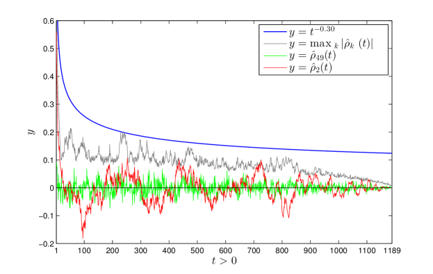
Figure 1: Sample autocorrelations of brain nodes.

Now take a look at the rfMRI data example of a single subject which will be further analyzed in Subsection 6.3. The data set consists of 1190 temporal brain images. We consider 907 functional brain nodes in each image. All node time series have passed the Priestley-Subba Rao test for stationarity [59], the generalized Jarque-Bera test for Gaussianity [2], and the Hinich’s bispectral test for linearity [44]. Hence the linear spatio-temporal model that we will define in the next subsection with sub-Gaussian tails seems adequate for the data. There are 134 time series detected as long-memory by the GPH test [38]. All these tests are conducted with a significant p-value of 0.05 adjusted by the false discovery rate controlling procedure of [7]. Hence, the weak temporal dependence models of [8, 9, 25] do not apply to these long-memory time series. For node $k$, its autocorrelation function $\rho_{k}(t):=\rho_{[k]}^{ij}$, $t=|i-j|$, can be approximated by the sample autocorrelation function $\hat{\rho}_{k}(t)$. Figure 1 shows that the rfMRI data approximately satisfy the PDD model (4) with $C_{0}=1$ and $\alpha=0.30$ since $\max_{1\leq k\leq p}|\hat{\rho}_{k}(t)|\leq t^{-0.30}$. The figure also illustrates the estimated autocorrelation functions for two randomly selected brain nodes, which clearly have different patterns, indicating that the assumption of homogeneous decay rates for all time series in [80] does not hold.

2.3 Data generating mechanism

Throughout the article, we assume that the vectorized data are obtained from the linear spatio-temporal model

$$\boldsymbol{X}_{pn}\coloneqq\text{vec}(\mathbf{X}_{p\times n})=\mathbf{H}\boldsymbol{e}+\boldsymbol{\mu}_{pn},$$ (7)

where $\mathbf{H}=(h_{ij})_{pn\times m}$ is a real deterministic matrix, $\boldsymbol{\mu}_{pn}=\boldsymbol{1}_{n}\otimes\boldsymbol{\mu}_{p}$, and the random vector $\boldsymbol{e}=(e_{1},\dots,e_{m})^{\top}$ consists of $m$ independent (not necessarily i.i.d.) random variables satisfying $E(e_{i})=0$ and $E(e_{i}^{2})=1$ for all $i$. We allow $m=\infty$ by requiring that for each $i$, $\sum_{j=1}^{m}h_{ij}e_{j}$ converges both almost surely and in mean square when $m\to\infty$. A sufficient and necessary condition for both modes of convergence is $\sum_{j=1}^{\infty}h_{ij}^{2}<\infty$ for every $i$ (see Theorem 8.3.4 and its proof in [1]). Under these two modes of convergence, it can be shown that $E(\mathbf{H}\boldsymbol{e})=\mathbf{H}E(\boldsymbol{e})$ and $\textup{Cov}(\mathbf{H}\boldsymbol{e})=\mathbf{H}\textup{Cov}(\boldsymbol{e})\mathbf{H}^{\top}$ (see Proposition 2.7.1 in [15]). Hence, for either finite or infinite $m$, we have $E(\boldsymbol{X}_{pn})=\boldsymbol{\mu}_{pn}$ and $\textup{Cov}(\boldsymbol{X}_{pn})=\mathbf{HH}^{\top}$ with all $n$ submatrices of dimension $p\times p$ on the diagonal equal to $\mathbf{\Sigma}$ and temporal correlations determined by the off-diagonal submatrices. In filtering theory, matrix $\mathbf{H}$ is said to be a linear spatio-temporal coloring filter [35, 55], which generates the output $\boldsymbol{X}_{pn}$ by introducing both spatial and temporal dependence in the input independent variables $e_{1},\dots,e_{m}$. We will use $\mathbf{X}_{p\times n}$ and $\boldsymbol{X}_{pn}$ exchangeably.

The following are two examples of (7) which are often seen in the literature. In particular, two processes used in analyzing fMRI data, i.e., the multivariate fractional Gaussian noise [28] and the vector autoregressive model [41], are special cases of these two examples, respectively.

Example 1 (Gaussian data).

Assume that $\boldsymbol{X}_{pn}$ has a multivariate Gaussian distribution $\mathcal{N}(\boldsymbol{\mu}_{pn},\mathbf{\Delta})$. Then $\mathbf{\Delta}=\mathbf{HH}$ with a symmetric real matrix $\mathbf{H}$. If $\mathbf{\Delta}\succ 0$, then $\boldsymbol{X}_{pn}=\mathbf{H}\boldsymbol{e}+\boldsymbol{\mu}_{pn}$ with $\boldsymbol{e}=\mathbf{H}^{-1}(\boldsymbol{X}_{pn}-\boldsymbol{\mu}_{pn})\sim\mathcal{N}(\boldsymbol{0},\mathbf{I}_{pn\times pn})$. If $\mathbf{\Delta}$ is singular, then $\boldsymbol{X}_{pn}$ has a degenerate multivariate Gaussian distribution, and can be expressed as $\boldsymbol{X}_{pn}\stackrel{{\scriptstyle d}}{{=}}\mathbf{H}\boldsymbol{e}+\boldsymbol{\mu}_{pn}$ with any $\boldsymbol{e}\sim\mathcal{N}(\boldsymbol{0},\mathbf{I}_{pn\times pn})$. In fact, replacing “$=$” in (7) by “$\stackrel{{\scriptstyle d}}{{=}}$” does not affect the theoretical results.

Example 2 (Moving average processes).

Consider the processes

$$\boldsymbol{X}_{j}=\sum_{\ell=0}^{L}\mathbf{B}_{\ell}\boldsymbol{e}_{j-\ell},\quad\text{with}\quad 0\leq L\leq\infty,$$ (8)

where the case with $L=\infty$ is well-defined in the sense of entrywise almost-sure convergence and mean-square convergence, $\{\mathbf{B}_{\ell}\}$ are $p\times p$ real deterministic matrices, and $\boldsymbol{e}_{j}=(e_{1j},e_{2j}\dots,e_{pj})^{\top}$ is a vector with independent zero-mean and unit-variance entries $\{e_{ij},1\leq i\leq p,\,-\infty\leq j\leq n\}$. Since every $X_{ij}$ is a linear combination of $\{e_{st}\}$, we always can find a matrix $\mathbf{H}$ such that $\boldsymbol{X}_{pn}=\mathbf{H}\boldsymbol{e}$ with $\boldsymbol{e}=(\boldsymbol{e}_{1-L}^{\top},\boldsymbol{e}_{2-L}^{\top},\dots,\boldsymbol{e}_{n}^{\top})^{\top}$. It is well-known that any causal vector autoregressive moving average process of the form $\boldsymbol{X}_{j}-\mathbf{A}_{1}\boldsymbol{X}_{j-1}-\dots-\mathbf{A}_{a}\boldsymbol{X}_{j-a}=\boldsymbol{e}_{j}+\mathbf{M}_{1}\boldsymbol{e}_{j-1}+\dots+\mathbf{M}_{b}\boldsymbol{e}_{j-b}$ with finite nonnegative integers $a$ and $b$, and real deterministic matrices $\{\mathbf{A}_{i},\mathbf{M}_{k}\}$, can be written in the form of (8) with $L=\infty$ [15, pp. 418]. Model (8) with $L=\infty$ is widely studied in recent literature of high dimensional time series (see, e.g., [25, 26, 9, 52]).

We will consider the following three types of moment conditions for the basis random variables $e_{1},\dots,e_{m}$ in (7), corresponding to sub-Gaussian, generalized sub-exponential, and polynomial-type tails, respectively. Let $Z$ be a random variable, and $K$, $\vartheta$, and $\eta_{k}$ be positive constants.

1. Sub-Gaussian tails: For all $k\geq 1$, we have $(E|Z|^{k})^{1/k}\leq Kk^{1/2}.$

2. Generalized sub-exponential tails: For some $\vartheta\in(0,2)$ and all $k\geq\vartheta$, we have $(E|Z|^{k})^{1/k}\leq K(k/\vartheta)^{1/\vartheta}.$

3. Polynomial-type tails: For some $k\geq 4$, we have $(E|Z|^{k})^{1/k}\leq\eta_{k}.$

We do not consider condition (C1) as a special case of condition (C2) by setting $\vartheta=2$ due to the fact that sharper convergence rates can be obtained under (C1). We can apply the Hanson-Wright inequality to (C1) [65], but not able to extend it to (C2) because the moment generating function of $Z^{2}$ is no longer finite in an open interval around zero (see Proposition 7.23 and inequality (7.32) in [36], and Lemma 5.5 in [72]). Conditions (C1) and (C2) can be equivalently written as $P(|Z|\geq u)\leq 2\exp(-u^{\vartheta}/C)$ with some constant $C>0$ for all $u\geq 0$, where for the former $\vartheta=2$. Condition (C3) implies $P(|Z|\geq u)\leq\eta_{k}^{k}/u^{k}$ for all $u>0$. Conversely, if $P(|Z|\geq u)=O(u^{-k^{\prime}})$ with some $k^{\prime}\in(0,k)$ as $u\to\infty$, then ${(E|Z|^{k})^{1/k}<\infty}$.

3 Estimation of covariance and correlation matrices for sub-Gaussian data

Consider the $\ell_{q}$-ball sparse covariance matrices [10, 63]

$$\mathcal{U}(q,c_{p},v_{0})=\bigg{\{}\mathbf{\Sigma}:\max_{1\leq i\leq p}\sum_{j=1}^{p}|\sigma_{ij}|^{q}\leq c_{p},\max_{1\leq i\leq p}\sigma_{ii}\leq v_{0}\bigg{\}},$$ (9)

and the corresponding correlation matrices

$$\mathcal{R}(q,c_{p})=\bigg{\{}\mathbf{R}:\max_{1\leq i\leq p}\sum_{j=1}^{p}|\rho_{ij}|^{q}\leq c_{p}\bigg{\}},$$ (10)

where constants $v_{0}>0$ and $0\leq q<1$. For any thresholding parameter $\tau\geq 0$, define a generalized thresholding function [63] by $s_{\tau}:\mathbb{R}\to\mathbb{R}$ satisfying the following conditions for all $z\in\mathbb{R}$: (i) $|s_{\tau}(z)|\leq|z|$; (ii) $s_{\tau}(z)=0$for $|z|\leq{\tau}$; (iii) $|s_{\tau}(z)-z|\leq{\tau}$. Such defined generalized thresholding function covers many widely used thresholding functions, including hard thresholding $s_{\tau}^{H}(z)=z\mathds{1}(|z|>{\tau}),$ soft thresholding $s_{\tau}^{S}(z)=\text{sign}(z)(|z|-{\tau})_{+},$ smoothly clipped absolute deviation and adaptive lasso thresholdings. See details about these examples in [63]. We define the generalized thresholding estimators of $\mathbf{\Sigma}$ and $\mathbf{R}$, respectively, by

$$S_{\tau_{1}}(\widehat{\mathbf{\Sigma}})=(s_{\tau_{1}}(\hat{\sigma}_{ij}))_{p\times p}\ \ \mbox{and}\ \ S_{\tau_{2}}(\widehat{\mathbf{R}})=\left(s_{\tau_{2}}(\hat{\rho}_{ij})\mathds{1}(i\neq j)+\mathds{1}(i=j)\right)_{p\times p},$$

where $\widehat{\mathbf{\Sigma}}\coloneqq(\hat{\sigma}_{ij})_{p\times p}$ is the sample covariance matrix given by

$$\widehat{\mathbf{\Sigma}}=\frac{1}{n}\sum_{i=1}^{n}\boldsymbol{X}_{i}\boldsymbol{X}_{i}^{\top}-\bar{\boldsymbol{X}}\bar{\boldsymbol{X}}^{\top}$$ (11)

with $\bar{\boldsymbol{X}}=\frac{1}{n}\sum_{i=1}^{n}\boldsymbol{X}_{i}$, and $\widehat{\mathbf{R}}\coloneqq\left(\hat{\rho}_{ij}\right)_{p\times p}=\left(\hat{\sigma}_{ij}/\sqrt{\hat{\sigma}_{ii}\hat{\sigma}_{jj}}\right)_{p\times p}$ is the sample correlation matrix. Define

$$u_{1}=\max\left\{(\log p)g_{2}/n,\ [(\log p)g_{F}/n]^{1/2}\right\}.$$ (12)

Then we have the following results.

Theorem 1.

Suppose that $\mathbf{X}_{p\times n}$ is generated from (7) with all $e_{i}$ satisfying condition (C1) with the same $K$. Uniformly on $\mathbf{\Sigma}\in\mathcal{U}(q,c_{p},v_{0})$ and $\{\mathbf{R}_{[k]}\}_{k=1}^{p}$ subject to (2), for sufficiently large constant $M_{1}>0$ depending only on $v_{0}$ and $K$, if ${\tau_{1}}=M_{1}u_{1}$ and $u_{1}=o(1)$, then

$$|S_{\tau_{1}}(\widehat{\mathbf{\Sigma}})-\mathbf{\Sigma}|_{\infty} =O_{P}(u_{1}),$$

$$\|S_{\tau_{1}}(\widehat{\mathbf{\Sigma}})-\mathbf{\Sigma}\|_{2} =O_{P}\left(c_{p}u_{1}^{1-q}\right),$$ (13)

$$\frac{1}{p}\|S_{\tau_{1}}(\widehat{\mathbf{\Sigma}})-\mathbf{\Sigma}\|_{F}^{2} =O_{P}\left(c_{p}u_{1}^{2-q}\right).$$ (14)

Moreover, if $p\geq n^{c}$ for some constant $c>0$, then with sufficiently large $M_{1}$ additionally depending on $c$ and $q$, we have

$$E\left(|S_{\tau_{1}}(\widehat{\mathbf{\Sigma}})-\mathbf{\Sigma}|_{\infty}^{2}\right) =O(u_{1}^{2}),$$

$$E\left(\|S_{\tau_{1}}(\widehat{\mathbf{\Sigma}})-\mathbf{\Sigma}\|_{2}^{2}\right) =O\left(c_{p}^{2}u_{1}^{2-2q}\right),$$

$$\frac{1}{p}E\left(\|S_{\tau_{1}}(\widehat{\mathbf{\Sigma}})-\mathbf{\Sigma}\|_{F}^{2}\right) =O\left(c_{p}u_{1}^{2-q}\right).$$

Remark 1.

When $(\log p)/n=o(1)$, if $u_{1}=O(\sqrt{(\log p)/n})$, which is true when $g_{2}<\infty$ that holds for short-memory multivariate time series satisfying (3), then the in-probability convergence rates given in (13) and (14) are the same rates as those for i.i.d. observations given in [10] and [63]. The same in-probability convergence rates are also obtained by [6, Proposition 5.1] for certain short-memory stationary Gaussian data using the hard thresholding method.

Remark 2.

For the PDD temporal dependence given in (4), by (5) and (6), together with $u_{1}=o(1)$, we have

$$u_{1}\lesssim\begin{cases}\sqrt{(\log p)/{n}},&\alpha>1;\\ \max\big{\{}[(\log p)(\log n)]/{n},\sqrt{(\log p)/{n}}\big{\}},&\alpha=1;\\ \max\big{\{}(\log p)/{n^{\alpha}},\sqrt{(\log p)/{n}}\big{\}},&\alpha\in(1/2,1);\\ \max\big{\{}(\log p)/{n^{1/2}},\sqrt{[(\log p)(\log n)]/{n}}\big{\}},&\alpha=1/2;\\ (\log p)/{n^{\alpha}},&\alpha\in(0,1/2).\end{cases}$$

Here $x_{n}\lesssim y_{n}$ denotes $x_{n}=O(y_{n})$. Note that the case with $\alpha>1$ is short-memory in the sense of (3). When $\alpha=1$ and $(\log n)\sqrt{(\log p)/n}=O(1)$, or when $\alpha\in(1/2,1)$ and $(\log p)^{1/2}n^{1/2-\alpha}=O(1)$, which allows some individual time series to be long-memory, we also have $u_{1}=O(\sqrt{(\log p)/n})$, yielding the same convergence rates as in the case with i.i.d. data.

Theorem 2 (Sparsistency and sign-consistency).

Under the conditions for the convergence in probability given in Theorem 1, we have ${s_{\tau_{1}}(\hat{\sigma}_{ij})=0}$ for all $(i,j)$ where $\sigma_{ij}=0$ with probability tending to 1. If further assume all nonzero entries of $\mathbf{\Sigma}$ satisfy $|\sigma_{ij}|\geq 2\tau_{1}$, then we have $\textup{sign}(s_{\tau_{1}}(\hat{\sigma}_{ij}))$ $=\textup{sign}(\sigma_{ij})$ for all $(i,j)$ where $\sigma_{ij}\neq 0$ with probability tending to 1.

Corollary 1.

Theorems 1 and 2 hold with $\widehat{\mathbf{\Sigma}},\mathbf{\Sigma},\hat{\sigma}_{ij},\sigma_{ij}$, $\mathcal{U}(q,c_{p},v_{0})$, $\tau_{1}$, and $M_{1}$ replaced by $\widehat{\mathbf{R}},\mathbf{R},\hat{\rho}_{ij},\rho_{ij}$, $\mathcal{R}(q,c_{p})$, $\tau_{2}$, and $M_{2}$, respectively, where $M_{2}$ does not depend on $v_{0}$.

We now provide the minimax optimal rates for estimating covariance and correlation matrices over certain sets of distributions of $\mathbf{X}_{p\times n}$, including the short-memory case (3) and some long-memory cases (4) with $\alpha\in(1/2,1]$.

Theorem 3 (Minimax rates).

Let $K_{G}=\sup_{k\geq 1}\sqrt{2/k}\left[\Gamma(\frac{1+k}{2})/\sqrt{\pi}\right]^{1/k}$, where $\Gamma(x)$ is the gamma function. Let $\mathcal{P}_{1}(q,c_{p},v_{0},g_{F},g_{2},K,\kappa)$ be the set of distributions of $\mathbf{X}_{p\times n}$ generated from (7) with all $e_{i}$ satisfying (C1) with constant $K\geq K_{G}$, $\mathbf{\Sigma}\in\mathcal{U}(q,c_{p},v_{0})$, and $\{\mathbf{R}_{[k]}\}_{k=1}^{p}$ subject to (2), where the constant ${\kappa\geq 1}$ is used in setting $u_{1}\leq\kappa\sqrt{(\log p)/n}$. Let $\mathcal{P}_{2}(q,c_{p},g_{F},g_{2},K,\kappa)$ be the corresponding set to $\mathcal{P}_{1}$ with $\mathbf{\Sigma}\in\mathcal{U}(q,c_{p},v_{0})$ replaced by $\mathbf{R}\in\mathcal{R}(q,c_{p})$. Let $\mathfrak{D}$ denote the distribution of $\mathbf{X}_{p\times n}$. If $\sqrt{(\log p)/n}=o(1)$,

$$p\geq n^{c_{1}}\quad\text{and}\quad c_{p}\leq c_{2}n^{(1-q)/2}(\log p)^{-(3-q)/2}$$ (15)

with some constants $c_{1}>1$ and $c_{2}>0$, then for any estimator $\widetilde{\mathbf{\Sigma}}$ we have

$$\inf_{\widetilde{\mathbf{\Sigma}}}\sup_{\mathfrak{D}\in\mathcal{P}_{1}}E_{\mathbf{X}_{p\times n}|\mathfrak{D}}\left(\|\widetilde{\mathbf{\Sigma}}-\mathbf{\Sigma}\|_{2}^{2}\right)\asymp c_{p}^{2}\left(\frac{\log p}{n}\right)^{1-q},$$

$$\inf_{\widetilde{\mathbf{\Sigma}}}\sup_{\mathfrak{D}\in\mathcal{P}_{1}}\frac{1}{p}E_{\mathbf{X}_{p\times n}|\mathfrak{D}}\left(\|\widetilde{\mathbf{\Sigma}}-\mathbf{\Sigma}\|_{F}^{2}\right)\asymp c_{p}\left(\frac{\log p}{n}\right)^{1-q/2}.$$

Additionally if $c_{p}>1$, then for any estimator $\widetilde{\mathbf{R}}$ we have

$$\inf_{\widetilde{\mathbf{R}}}\sup_{\mathfrak{D}\in\mathcal{P}_{2}}E_{\mathbf{X}_{p\times n}|\mathfrak{D}}\left(\|\widetilde{\mathbf{R}}-\mathbf{R}\|_{2}^{2}\right)\asymp c_{p}^{2}\left(\frac{\log p}{n}\right)^{1-q},$$

$$\inf_{\widetilde{\mathbf{R}}}\sup_{\mathfrak{D}\in\mathcal{P}_{2}}\frac{1}{p}E_{\mathbf{X}_{p\times n}|\mathfrak{D}}\left(\|\widetilde{\mathbf{R}}-\mathbf{R}\|_{F}^{2}\right)\asymp c_{p}\left(\frac{\log p}{n}\right)^{1-q/2}.$$

For sufficiently large positive constants $M_{1}$ and $M_{2}$, with $\tau_{1}=M_{1}u_{1}$ and $\tau_{2}=M_{2}u_{1}$, the generalized thresholding estimators $S_{\tau_{1}}(\widehat{\mathbf{\Sigma}})$ and $S_{\tau_{2}}(\widehat{\mathbf{R}})$ attain the above minimax optimal rates, respectively.

The assumption (15) follows [23] who studied the minimax optimal rates of the covariance matrix estimation for i.i.d. data. From Remarks 1 and 2 we see that suitable $(g_{F},g_{2},\kappa)$ in $\mathcal{P}_{1}$ and $\mathcal{P}_{2}$ allow $\mathbf{X}_{p\times n}$ to have short memory (3), or to follow the PDD model (4) with $\alpha\in(1/2,1]$ (thus with some time series to be long-memory) under some additional conditions for $n$ and $p$ discussed in Remark 2.

4 Estimation of precision matrix for sub-Gaussian data

We consider both the CLIME and the SPICE methods for the estimation of $\mathbf{\Omega}$, which were originally developed for i.i.d. observations.

4.1 CLIME estimation

Following [19], we consider the following set of precision matrices

$$\mathcal{G}_{1}(q,c_{p},M_{p},v_{0}){=}\Big{\{}\boldsymbol{\Omega}\succ 0:\max_{1\leq i\leq p}\sum_{j=1}^{p}|\omega_{ij}|^{q}\leq c_{p},\|\boldsymbol{\Omega}\|_{1}\leq M_{p},\max_{1\leq i\leq p}\sigma_{ii}\leq v_{0}\Big{\}},$$

where constant $0\leq q<1$, and $(c_{p},M_{p})$ are allowed to depend on $p$. Though the condition $\max_{i}\sigma_{ii}\leq v_{0}$ is not explicitly provided by [19] in their original set definition, it is implied by their moment conditions (see their (C1) and (C2)). Note that the above ${\cal G}_{1}$ contains $\ell_{q}$-ball sparse matrices such as those with exponentially decaying entries from the diagonal, for example, AR(1) matrices. For an invertible band matrix $\mathbf{\Sigma}$, its inverse matrix $\mathbf{\Omega}$ generally has exponentially decaying entries from the diagonal [31].

Let $\widehat{\mathbf{\Theta}}_{\varepsilon,\lambda_{1}}\coloneqq(\hat{\theta}_{ij}^{(\varepsilon,\lambda_{1})})_{p\times p}$ be a solution of the following optimization:

$$\min|\mathbf{\Theta}|_{1}\quad\mbox{subject to}\quad|\widetilde{\mathbf{\Sigma}}_{\varepsilon}\mathbf{\Theta}-\mathbf{I}_{p\times p}|_{\infty}\leq\lambda_{1},\quad\mathbf{\Theta}\in\mathbb{R}^{p\times p},$$ (16)

where $\widetilde{\boldsymbol{\Sigma}}_{\varepsilon}=\widehat{\boldsymbol{\Sigma}}+\varepsilon\mathbf{I}_{p\times p}$, $\widehat{\boldsymbol{\Sigma}}$ is given in (11), $\varepsilon\geq 0$ is a perturbation parameter introduced for the same reasons given in [19] and can be set to be $n^{-1/2}$ in practice (see Remark 4 below), and $\lambda_{1}$ is a tuning parameter. The CLIME estimator $\widehat{\mathbf{\Omega}}_{\varepsilon,\lambda_{1}}\coloneqq(\hat{\omega}_{ij}^{(\varepsilon,\lambda_{1})})_{p\times p}$ is then obtained by symmetrizing $\widehat{\mathbf{\Theta}}_{\varepsilon,\lambda_{1}}$ with

$$\hat{\omega}_{ij}^{(\varepsilon,\lambda_{1})}=\hat{\omega}_{ji}^{(\varepsilon,\lambda_{1})}=\hat{\theta}_{ij}^{(\varepsilon,\lambda_{1})}\mathds{1}(|\hat{\theta}_{ij}^{(\varepsilon,\lambda_{1})}|\leq|\hat{\theta}_{ji}^{(\varepsilon,\lambda_{1})}|)+\hat{\theta}_{ji}^{(\varepsilon,\lambda_{1})}\mathds{1}(|\hat{\theta}_{ij}^{(\varepsilon,\lambda_{1})}|>|\hat{\theta}_{ji}^{(\varepsilon,\lambda_{1})}|).$$

For $1\leq i\leq p$, let $\hat{\boldsymbol{\beta}}_{i}^{(\varepsilon,\lambda_{1})}$ be a solution of the following convex optimization problem:

$$\min|\boldsymbol{\beta}_{i}|_{1}\quad\mbox{subject to}\quad|\widetilde{\mathbf{\Sigma}}_{\varepsilon}\boldsymbol{\beta}_{i}-\boldsymbol{e}_{i}|_{\infty}\leq\lambda_{1},$$ (17)

where $\boldsymbol{\beta}_{i}$ is a real vector and $\boldsymbol{e}_{i}$ is the vector with 1 in the $i$-th coordinate and 0 in all other coordinates. [19] showed that solving the optimization problem (16) is equivalent to solving the $p$ optimization problems given in (17), i.e., $\widehat{\mathbf{\Theta}}_{\varepsilon,\lambda_{1}}=(\hat{\boldsymbol{\beta}}_{1}^{(\varepsilon,\lambda_{1})},\dots,\hat{\boldsymbol{\beta}}_{p}^{(\varepsilon,\lambda_{1})})$. This equivalence is useful for both numerical implementation and theoretical analysis. The following theorem gives the convergence results of CLIME under temporal dependence.

Theorem 4.

Suppose that $\mathbf{X}_{p\times n}$ is generated from (7) with all $e_{i}$ satisfying condition (C1) with the same $K$. Uniformly on $\mathbf{\Omega}\in\mathcal{G}_{1}(q,c_{p},M_{p},v_{0})$ and $\{\mathbf{R}_{[k]}\}_{k=1}^{p}$ subject to (2), for sufficiently large constant $M>0$ depending only on $v_{0}$ and $K$, if ${\lambda_{1}}=MM_{p}u_{1}$, $0\leq\varepsilon\leq u_{1}$ and $u_{1}=o(1)$ with $u_{1}$ defined in (12), then

$$|\widehat{\mathbf{\Omega}}_{\varepsilon,\lambda_{1}}-\boldsymbol{\Omega}|_{\infty} =O_{P}(M_{p}^{2}u_{1}),$$

$$\|\widehat{\mathbf{\Omega}}_{\varepsilon,\lambda_{1}}-\boldsymbol{\Omega}\|_{2} =O_{P}\left(c_{p}(M_{p}^{2}u_{1})^{1-q}\right),$$

$$\frac{1}{p}\|\widehat{\mathbf{\Omega}}_{\varepsilon,\lambda_{1}}-\boldsymbol{\Omega}\|_{F}^{2} =O_{P}\left(c_{p}(M_{p}^{2}u_{1})^{2-q}\right).$$

Moreover, if $p\geq n^{c}$ and $\min\{p^{-C},u_{1}\}\leq\varepsilon\leq u_{1}$ for some positive constants $c$ and $C$, then with sufficiently large $M$ additionally depending on $c,C$ and $q$, we have

$$E\left(|\widehat{\mathbf{\Omega}}_{\varepsilon,\lambda_{1}}-\boldsymbol{\Omega}|_{\infty}^{2}\right) =O\left((M_{p}^{2}u_{1})^{2}\right),$$

$$E\left(\|\widehat{\mathbf{\Omega}}_{\varepsilon,\lambda_{1}}-\boldsymbol{\Omega}\|_{2}^{2}\right) =O\left(c_{p}^{2}(M_{p}^{2}u_{1})^{2-2q}\right),$$ (18)

$$\frac{1}{p}E\left(\|\widehat{\mathbf{\Omega}}_{\varepsilon,\lambda_{1}}-\boldsymbol{\Omega}\|_{F}^{2}\right) =O\left(c_{p}(M_{p}^{2}u_{1})^{2-q}\right).$$ (19)

Remark 3.

If $(\log p)/n=o(1)$ and $u_{1}=O(\sqrt{(\log p)/n})$, then the above convergence rates are the same as those for i.i.d. data given in [19]. Additionally, if $M_{p}$ is a constant, then the mean-square convergence rates of CLIME in (18) and (19) attain the minimax optimal convergence rates for i.i.d. data shown in [20] under slightly different assumptions. From Remarks 1 and 2 we see that $u_{1}=O(\sqrt{(\log p)/n})$ when $u_{1}=o(1)$ can be achieved for the short-memory case (3) and also for the long-memory cases satisfying (4) with $\alpha\in(1/2,1]$ under some additional conditions for $n$ and $p$.

Remark 4.

As discussed in [19], the perturbation parameter $\varepsilon>0$ is used for a proper initialization of $\{\boldsymbol{\beta}_{i}\}$ in the numerical implementation of (17), and also ensures the existence of $E(\|\widehat{\mathbf{\Omega}}_{\varepsilon,\lambda_{1}}-\boldsymbol{\Omega}\|_{2}^{2})$. Since $g_{F}\geq 1$, from (12) we have that $u_{1}\geq\sqrt{(\log p)/n}\geq n^{-1/2}$. Hence when $p\geq n^{c}$, let $C=1/(2c)$, we have $p^{-C}\leq n^{-1/2}\leq u_{1}$. Thus, we can simply let $\varepsilon=n^{-1/2}$ in practice, which is also the default setting of the R package flare [51] that implements the CLIME algorithm. The same choice of $\varepsilon$ is given in (10) of [19] for i.i.d. observations.

To better recover the sparsity structure of $\mathbf{\Omega}$, [19] introduced additional thresholding on $\widehat{\mathbf{\Omega}}_{\varepsilon,\lambda_{1}}$. Similarly, we may define a hard-thresholded CLIME estimator $\widetilde{\mathbf{\Omega}}_{\varepsilon,\lambda_{1},\xi}=(\tilde{\omega}_{ij}^{(\varepsilon,\lambda_{1},\xi)})_{p\times p}$ by $\tilde{\omega}_{ij}^{(\varepsilon,\lambda_{1},\xi)}=\hat{\omega}_{ij}^{(\varepsilon,\lambda_{1})}\mathds{1}(|\hat{\omega}_{ij}^{(\varepsilon,\lambda_{1})}|>\xi)$ with a tuning parameter $\xi\geq 4M_{p}\lambda_{1}$. Although such an estimator enjoys nice theoretical properties given below, how to practically select $\xi$ remains unknown.

Theorem 5 (Sparsistency and sign-consistency).

Under the conditions for the convergence in probability given in Theorem 4, we have $\tilde{\omega}_{ij}^{(\varepsilon,\lambda_{1},\xi)}=0$ for all $(i,j)$ where $\omega_{ij}=0$ with probability tending to 1. If further assume all nonzero entries of $\boldsymbol{\Omega}$ satisfy $|\omega_{ij}|>\xi+4M_{p}\lambda_{1}$, then we have $\textup{sign}(\tilde{\omega}_{ij}^{(\varepsilon,\lambda_{1},\xi)})=\textup{sign}(\omega_{ij})$ for all $(i,j)$ where $\omega_{ij}\neq 0$ with probability tending to 1.

4.2 SPICE estimation

For i.i.d. observations, [62] proposed the SPICE method for estimating the following precision matrix $\mathbf{\Omega}$

$$\mathcal{G}_{2}(s_{p},v_{0}){=}\Big{\{}\mathbf{\Omega}:\sum_{1\leq i\neq j\leq p}\mathds{1}(\omega_{ij}\neq 0)\leq s_{p},0{<}v_{0}^{-1}{\leq}\varphi_{\min}(\mathbf{\Omega}){\leq}\varphi_{\max}(\mathbf{\Omega}){\leq}v_{0}\Big{\}},$$

where $s_{p}$ determines the sparsity of $\mathbf{\Omega}$ and can depend on $p$, and $v_{0}$ is a constant. Two types of SPICE estimators were proposed:

$$\widetilde{\mathbf{\Omega}}_{\lambda_{2}}=\operatorname*{arg\,min}_{\begin{subarray}{c}{\mathbf{\Theta}}\succ 0,{\mathbf{\Theta}}={\mathbf{\Theta}}^{\top}\end{subarray}}\left\{\text{tr}(\mathbf{\Theta}\widehat{\mathbf{\Sigma}})-\log\det(\mathbf{\Theta})+\lambda_{2}|\mathbf{\Theta}|_{1,\text{off}}\right\},$$ (20)

and

$$\widehat{\mathbf{\Omega}}_{\lambda_{2}} \coloneqq(\hat{\omega}_{ij}^{(\lambda_{2})})_{p\times p}=\widehat{\mathbf{W}}^{-1}\widehat{\mathbf{K}}_{\lambda_{2}}\widehat{\mathbf{W}}^{-1}\quad\text{with}$$ (21)

$$\widehat{\mathbf{K}}_{\lambda_{2}} =\operatorname*{arg\,min}_{\begin{subarray}{c}{\mathbf{\Theta}}\succ 0,{\mathbf{\Theta}}={\mathbf{\Theta}}^{\top}\end{subarray}}\left\{\text{tr}(\mathbf{\Theta}\widehat{\mathbf{R}})-\log\det(\mathbf{\Theta})+\lambda_{2}|\mathbf{\Theta}|_{1,\text{off}}\right\},$$

where $\lambda_{2}>0$ is a tuning parameter, and $\widehat{\mathbf{W}}={\rm diag}\{\sqrt{\hat{\sigma}_{11}},\dots,\sqrt{\hat{\sigma}_{pp}}\}$. We can see that $\widehat{\mathbf{K}}_{\lambda_{2}}$ is the SPICE estimator of $\mathbf{K}\coloneqq\mathbf{R}^{-1}$. The SPICE estimator (20) is a slight modification of the graphical Lasso (GLasso) estimator of [37]. GLasso uses $|\mathbf{\Omega}|_{1}$ rather than $|\mathbf{\Omega}|_{1,\text{off}}$ in the penalty, but the SPICE estimators (20) and (21) are more amenable to theoretical analysis [50, 61, 62], and numerically they give similar results for i.i.d. data [62]. It is worth noting that for i.i.d. data, (20) requires $\sqrt{(p+s_{p})(\log p)/n}=o(1)$ but (21) relaxes it to $\sqrt{(1+s_{p})(\log p)/n}=o(1)$. Similar requirements also hold for temporally dependent observations. Hence in this article, we only consider the SPICE estimator given in (21).

Theorem 6.

Suppose that $\mathbf{X}_{p\times n}$ is generated from (7) with all $e_{i}$ satisfying condition (C1) with the same $K$. Uniformly on $\mathbf{\Omega}\in\mathcal{G}_{2}(s_{p},v_{0})$ and $\{\mathbf{R}_{[k]}\}_{k=1}^{p}$ subject to (2), for sufficiently large constant $M>0$ depending only on $v_{0}$ and $K$, if ${\lambda_{2}}=Mu_{1}$ and $u_{1}=o(1/\sqrt{1+s_{p}})$ with $u_{1}$ defined in (12), then we have

$$\|\widehat{\mathbf{K}}_{\lambda_{2}}-\mathbf{K}\|_{F} =O_{P}(u_{1}\sqrt{s_{p}}),$$

$$\|\widehat{\mathbf{\Omega}}_{\lambda_{2}}-\mathbf{\Omega}\|_{2} =O_{P}(u_{1}\sqrt{1+s_{p}}),$$

$$\frac{1}{\sqrt{p}}\|\widehat{\mathbf{\Omega}}_{\lambda_{2}}-\mathbf{\Omega}\|_{F} =O_{P}\left(u_{1}\sqrt{1+s_{p}/p}\right).$$

Again by Remarks 1 and 2, $u_{1}=O(\sqrt{(\log p)/n})$ is achievable for the short-memory case (3) and also for some long-memory cases, thus for such temporally dependent data Theorem 6 gives the same convergence rates as those given in [62] for i.i.d. observations. The condition $u_{1}=o(1/\sqrt{1+s_{p}})$ implies $s_{p}=o(u_{1}^{-2})=o(n/\log p)$, meaning that $\mathbf{\Omega}$ needs to be very sparse. Such a condition easily fails for many simple band matrices when $p\geq n$.

Under the irrepresentability condition, however, the sparsity requirement can be relaxed [61]. In particular, define $\mathbf{\Gamma}=\mathbf{R}\otimes\mathbf{R}$. By $(i,j)$-th row of $\mathbf{\Gamma}$ we refer to its $[i+(j-1)p]$-th row, and by $(k,\ell)$-th column to its $[k+(\ell-1)p]$-th column. For any two subsets $T$ and $T^{\prime}$ of $\{1,...,p\}{\times}\{1,...,p\}$, denote $\mathbf{\Gamma}_{TT^{\prime}}$ be the $\text{card}(T){\times}\text{card}(T^{\prime})$ matrix with rows and columns of $\mathbf{\Gamma}$ indexed by $T$ and $T^{\prime}$ respectively, where $\text{card}(T)$ denotes the cardinality of set $T$. Let $S$ be the set of nonzero entries of $\mathbf{\Omega}$ and $S^{c}$ be the complement of $S$ in $\{1,...,p\}{\times}\{1,...,p\}$. Define $\kappa_{\mathbf{R}}=\|\mathbf{R}\|_{1}$ and $\kappa_{\mathbf{\Gamma}}=\|\mathbf{\Gamma}_{SS}^{-1}\|_{1}$. Assume the following irrepresentability condition of [61]:

$$\max_{e\in S^{c}}\left|\mathbf{\Gamma}_{eS}\mathbf{\Gamma}_{SS}^{-1}\right|_{1}\leq 1-\beta$$ (22)

for some $\beta\in(0,1]$. Define $d$ to be the maximum number of nonzeros per row in $\mathbf{\Omega}$. Then we have the following result.

Theorem 7.

Let $r=\left(0.5+2.5(1+8/\beta)\kappa_{\mathbf{\Gamma}}\right)Mu_{1}v_{0}$, where $u_{1}$ is defined in (12). Suppose that $\mathbf{X}_{p\times n}$ is generated from (7) with all $e_{i}$ satisfying condition (C1) with the same $K$. Uniformly on $\mathbf{\Omega}\in\mathcal{G}_{2}(s_{p},v_{0})$ and $\{\mathbf{R}_{[k]}\}_{k=1}^{p}$ subject to (2), for sufficiently large constant $M>0$ depending on $v_{0}$ and $K$, if $\lambda_{2}=8Mu_{1}/\beta\leq[6(1+\beta/8)d\max\{\kappa_{\mathbf{R}}\kappa_{\mathbf{\Gamma}},\kappa_{\mathbf{R}}^{3}\kappa_{\mathbf{\Gamma}}^{2}\}]^{-1}$ and $u_{1}=o(\min\{1,[(1+8/\beta)\kappa_{\mathbf{\Gamma}}]^{-1}\})$, then with probability tending to 1 we have

$$|\widehat{\mathbf{\Omega}}_{\lambda_{2}}-\mathbf{\Omega}|_{\infty} \leq r,$$

$$\|\widehat{\mathbf{\Omega}}_{\lambda_{2}}-\mathbf{\Omega}\|_{2} \leq r\min\left\{d,\sqrt{p+s_{p}}\right\},$$

$$\frac{1}{\sqrt{p}}\|\widehat{\mathbf{\Omega}}_{\lambda_{2}}-\mathbf{\Omega}\|_{F} \leq r\sqrt{1+s_{p}/p},$$

and $\hat{\omega}_{ij}^{(\lambda_{2})}=0$ for all $(i,j)$ with $\omega_{ij}=0$. If we further assume all nonzero entries of $\boldsymbol{\Omega}$ satisfy $|\omega_{ij}|>r$, then with probability tending to 1, $\textup{sign}(\hat{\omega}_{ij}^{(\lambda_{2})})=\textup{sign}(\omega_{ij})$ for all $(i,j)$ where $\omega_{ij}\neq 0$.

Consider the case when $\beta$ remains constant and $\max\{\kappa_{\mathbf{R}},\kappa_{\mathbf{\Gamma}}\}$ has a constant upper bound. Then the conditions in Theorem 7 about $\lambda_{2}$ and $u_{1}$ reduce to $\lambda_{2}=M^{\prime}u_{1}$ and $u_{1}=o(1)$ with a constant $M^{\prime}=8M/\beta$, and meanwhile we have $\|\widehat{\mathbf{\Omega}}_{\lambda_{2}}-\mathbf{\Omega}\|_{2}=O_{P}(u_{1}d).$ Then the desired result of $\|\widehat{\mathbf{\Omega}}_{\lambda_{2}}-\mathbf{\Omega}\|_{2}=o_{P}(1)$ is achieved under a relaxed sparsity condition $d=o(u_{1}^{-1})$. If $d^{2}>1+s_{p}$, then $s_{p}=o(u_{1}^{-2})$ and the condition of Theorem 6 satisfies. Hence $\|\widehat{\mathbf{\Omega}}_{\lambda_{2}}-\mathbf{\Omega}\|_{2}=O_{P}(u_{1}\sqrt{\min\{d^{2},1+s_{p}\}})=o_{P}(1),$ which is the better rate between those from Theorems 6 and 7.

5 Extension to heavy tail data

In this section, we generalize the theoretical results for sub-Gaussian data to the cases when all the basis random variables $\{e_{i}\}$ have the generalized sub-exponential tails under condition (C2) or the polynomial-type tails under condition (C3). Define

$$u_{2}=\max\left\{(\log p)^{1+2/\vartheta}g_{2}/n,(\log p)^{1+2/\vartheta}(g_{F}/n)^{1/2}\right\},$$ (23)

and

$$u_{3}=\max\left\{p^{(2+2C)/k}g_{2}/n,p^{(4+2C)/k}(g_{F}/n)^{1/2}\right\}$$ (24)

with an arbitrary constant $C>0$. The quantities $u_{2}$ and $u_{3}$ will substitute $u_{1}$ in characterizing the matrix estimation convergence rates under the tail conditions  (C2) and (C3), respectively. The first term in either $u_{2}$ or $u_{3}$ can be dropped if $\boldsymbol{\mu}_{p}$ is known thus no need to be estimated.

Theorem 8 (Generalized sub-exponential tails).

Theorems 1, 2, 4$-$7, and Corollary 1 hold with condition (C1), parameter $K$, and $u_{1}$ replaced by condition (C2), parameters $\{K,\vartheta\}$, and $u_{2}$, respectively.

Theorem 9 (Polynomial-type tails).

Theorems 1, 2, 4$-$7, and Corollary 1, except those mean-square convergence results therein, hold with condition (C1), parameter $K$, and $u_{1}$ replaced by condition (C3), parameters $\{k,\eta_{k}\}$, and $u_{3}$, respectively.

For data with polynomial-type tails, the mean-square convergence results may require higher order moment conditions, thus are not pursued here.

A referee pointed out a potential connection to the recent work of [26], where the estimation of $\mathbf{\Omega}\boldsymbol{b}$ with $\boldsymbol{b}\in\mathbb{R}^{p}$ was considered for high-dimensional mean-zero stationary processes given in (8) with a temporal dependence satisfying PDD given in $\eqref{PDD}$. Our exploration shows that their concentration inequalities (see page 3 of their Supplementary Material) can be used to obtain the same convergence rates for our concerned estimators to their sub-Gaussian time series. Together with the concentration inequalities in [76], their inequalities also can be applied to their time series with the generalized sub-exponential tails, but result in slower convergence rates. If applied to their time series data with polynomial-type tails, however, their inequalities seem to yield faster convergence rates than ours. We leave the details to interested readers. Note that it is not clear if the concentration inequalities in [26] and [76] are applicable to the more general temporal dependence that we consider here in this article.

6 Numerical Results

6.1 Gap-block cross-validation

For tuning parameter selection, we propose a gap-block cross-validation method that includes the following steps:

1. Split the data $\mathbf{X}_{p\times n}$ into $H_{1}\geq 4$ approximately equal-sized non-overlapping blocks $\mathbf{X}^{*}_{i}$, $i=1,\dots,H_{1}$, such that $\mathbf{X}_{p\times n}=(\mathbf{X}_{1}^{*},\mathbf{X}_{2}^{*},\dots,\mathbf{X}_{H_{1}}^{*})$. For each $i$, set aside block $\mathbf{X}_{i}^{*}$ that will be used as the validation data, and use the remaining data after further dropping the neighboring blocks at both sides of $\mathbf{X}_{i}^{*}$ as the training data that are denoted by $\mathbf{X}_{i}^{**}$.

2. Randomly sample $H_{2}$ blocks $\mathbf{X}_{H_{1}+1}^{*},\dots,\mathbf{X}_{H_{1}+H_{2}}^{*}$ from $\mathbf{X}_{p\times n}$, where $\mathbf{X}_{H_{1}+j}^{*}$ consists of $\lceil{n/H_{1}}\rceil$ consecutive columns of $\mathbf{X}_{p\times n}$ for each $j=1,\dots,H_{2}$. Note that these sampled blocks can overlap. For each $i=H_{1}+1,\dots,H_{1}+H_{2}$, set aside block $\mathbf{X}_{i}^{*}$ as the validation data, and use the remaining data by further excluding the $\lceil{n/H_{1}}\rceil$ columns at both sides of $\mathbf{X}_{i}^{*}$ from $\mathbf{X}_{p\times n}$ as the training data that are denoted by $\mathbf{X}_{i}^{**}$.

3. Let $H=H_{1}+H_{2}$. Select the optimal values of tuning parameters $\tau_{1},\tau_{2},\lambda_{1}$ and $\lambda_{2}$ among their corresponding prespecified candidate values $\{\tau_{1j}\}_{j=1}^{J}$, $\{\tau_{2j}\}_{j=1}^{J}$, $\{\lambda_{1j}\}_{j=1}^{J}$ and $\{\lambda_{2j}\}_{j=1}^{J}$, and denote them respectively by

   $$\hat{\tau}_{1} =\mathop{\arg\min}_{1\leq j\leq J}\frac{1}{H}\sum_{i=1}^{H}\|S_{{\tau}_{1j}}(\widehat{\mathbf{\Sigma}}_{i}^{**})-\widehat{\mathbf{\Sigma}}_{i}^{*}\|_{F}^{2},$$

   $$\hat{\tau}_{2} =\mathop{\arg\min}_{1\leq j\leq J}\frac{1}{H}\sum_{i=1}^{H}\|S_{{\tau}_{2j}}(\widehat{\mathbf{R}}_{i}^{**})-\widehat{\mathbf{R}}_{i}^{*}\|_{F}^{2},$$

   $$\hat{\lambda}_{1} =\mathop{\arg\min}_{1\leq j\leq J}\frac{1}{H}\sum_{i=1}^{H}\left[\text{tr}(\widehat{\mathbf{\Omega}}_{\varepsilon,\lambda_{1j},i}^{**}\widehat{\mathbf{\Sigma}}_{i}^{*})-\log\det(\widehat{\mathbf{\Omega}}_{\varepsilon,\lambda_{1j},i}^{**})\right],$$

   $$\hat{\lambda}_{2} =\mathop{\arg\min}_{1\leq j\leq J}\frac{1}{H}\sum_{i=1}^{H}\left[\text{tr}(\widehat{\mathbf{\Omega}}_{\lambda_{2j},i}^{**}\widehat{\mathbf{\Sigma}}_{i}^{*})-\log\det(\widehat{\mathbf{\Omega}}_{\lambda_{2j},i}^{**})\right],$$

   where $\widehat{\mathbf{\Sigma}}_{i}^{*}$ and $\widehat{\mathbf{R}}_{i}^{*}$ are obtained from $\mathbf{X}_{i}^{*}$, $\widehat{\mathbf{\Sigma}}_{i}^{**}$ and $\widehat{\mathbf{R}}_{i}^{**}$ are obtained from $\mathbf{X}_{i}^{**}$, and $\widehat{\mathbf{\Omega}}_{\varepsilon,\lambda_{1j},i}^{**}$ and $\widehat{\mathbf{\Omega}}_{\lambda_{2j},i}^{**}$ are the CLIME and SPICE estimators, respectively, obtained from $\mathbf{X}_{i}^{**}$.

In the above cross-validation (CV), due to lack of independent observations, we use gap blocks, each of size $\approx\lceil{n/H_{1}}\rceil$, to separate training and validation datasets so that they are nearly uncorrelated. The idea of using gap blocks has been employed by the $hv$-block CV of [60] for linear models with dependent data. Similar to the $k$-fold CV for i.i.d. data, Step 1 guarantees all observations are used for both training and validation, but is limited due to the constrain of keeping the temporal ordering of the observations. Step 2 allows more data splits. This is particularly useful when Step 1 only allows a small number of data splits due to large-size of the gap block and/or limited sample size $n$. Step 2 is inspired by the commonly used repeated random subsampling CV for i.i.d. observations [68]. The above loss functions for selecting tuning parameters are widely used in the literature [10, 19, 20, 63]. The theoretical justification for the gap-block CV remains open. In our numerical examples, we simply set $H_{1}=H_{2}=10$, mimicing the $10$-fold CV recommended by [34, 42]. Our simulation studies show that the method performs well for temporally dependent data.

6.2 Simulation studies

We evaluate the numerical performance of the hard and soft thresholding estimators for large correlation matrix and the CLIME and SPICE estimators for large precision matrix. We generate Gaussian data with zero mean and covariance matrix $\mathbf{\Sigma}$ or precision matrix $\mathbf{\Omega}$ from one of the following four models:

1. $\sigma_{ij}=0.6^{|i-j|}$;

2. $\sigma_{ii}=1$, $\sigma_{i,i+1}=\sigma_{i+1,i}=0.6$, $\sigma_{i,i+2}=\sigma_{i+2,i}=0.3$, and $\sigma_{ij}=0$ for $|i-j|\geq 3$;

3. $\omega_{ij}=0.6^{|i-j|}$;

4. $\omega_{ii}=1$, $\omega_{i,i+1}=\omega_{i+1,i}=0.6$, $\omega_{i,i+2}=\omega_{i+2,i}=0.3$, and $\omega_{ij}=0$ for $|i-j|\geq 3$.

Similar models have been considered in [10, 19, 20, 62, 63]. For the temporal dependence, we set $\textup{Corr}(X_{ki},X_{\ell j})=\varLambda_{k\ell}^{ij}\rho_{k\ell}$ with

$$\varLambda_{k\ell}^{ij}=(|i-j|+1)^{-\alpha},\quad 1\leq i,j\leq n,$$ (25)

so that $\rho_{[k]}^{ij}\sim|i-j|^{-\alpha}$. It is computationally expensive to simulate data $\boldsymbol{X}_{pn}$ directly from a multivariate Gaussian random number generator because of the large dimension of its covariance matrix $\textup{Cov}(\boldsymbol{X}_{pn})$. Instead, we simulate data using the method of [13], which approximately satisfy (25) (see details in Supplementary Material).

Simulations are conducted with sample size $n=200$, variable dimension $p$ ranging from 100 to 400, and 100 replications under each setting, for which $\alpha$ varies from 0.1 to 2. The i.i.d. case is also considered, for which an ordinary 10-fold CV is implemented. For each simulated data set, we choose the optimal tuning parameter from a set of 50 specified values (see Section S.4.1 in Supplementary Material). The CLIME and SPICE are computed by the R packages flare [51] and QUIC [46], respectively. For CLIME, we use the default perturbation of flare with $\varepsilon=n^{-1/2}$.

The estimation performance is measured by both the spectral norm and the Frobenius norm. True-positive rate (TPR) and false-positive rate (FPR) are used for evaluating sparsity recovering for the correlation matrix:

$$\text{TPR}=\frac{\#\{(i,j):s_{\tau}(\hat{\rho}_{ij})\neq 0\ \text{and}\ \rho_{ij}\neq 0,i\neq j\}}{\#\{(i,j):\rho_{ij}\neq 0,i\neq j\}},$$

$$\text{FPR}=\frac{\#\{(i,j):s_{\tau}(\hat{\rho}_{ij})\neq 0\ \text{and}\ \rho_{ij}=0,i\neq j\}}{\#\{(i,j):\rho_{ij}=0,i\neq j\}}.$$

Similar quantities are also reported for the precision matrix. The TPR and FPR are not provided for Models 1 and 3.

Simulation results are summarized in Tables 1-3. In all setups, the sample correlation matrix and the inverse of sample covariance matrix (whenever possible) perform the worst. It is not surprising that the performance of all the regularized estimators generally is better for weaker temporal dependence or smaller $p$. The soft thresholding method performs slightly better than the hard thresholding method in terms of matrix losses for small $\alpha$ and slightly worse for large $\alpha$, and always has higher TPRs but bigger FPRs. The CLIME estimator performs similarly as the SPICE estimator in matrix norms, but generally yields lower FPRs.

We notice that the SPICE algorithm in the R package QUIC is much faster than the CLIME algorithm in the R package flare by using a single computer core. However, the column-by-column estimating nature of CLIME can speed up using parallel computing on multiple cores.

Table 1: Comparison of average (SD) matrix losses for correlation matrix estimation

$p$	$\ \alpha$		$\widehat{\mathbf{R}}\quad\$	Hard	Soft		$\widehat{\mathbf{R}}\quad\$	Hard	Soft
			Spectral norm				Frobenius norm
			Model 1
100	0.1		13.7(1.68)	2.8(0.09)	2.6(0.07)		22.6(1.08)	9.9(0.28)	8.7(0.24)
	0.25		10.5(1.59)	2.4(0.15)	2.4(0.08)		17.4(0.95)	8.1(0.42)	7.5(0.26)
	0.5		7.8(1.14)	2.0(0.15)	2.2(0.08)		14.3(0.69)	6.8(0.33)	6.6(0.23)
	1		4.2(0.45)	1.5(0.10)	1.7(0.08)		9.9(0.29)	5.2(0.23)	5.1(0.20)
	2		2.6(0.24)	1.1(0.09)	1.4(0.08)		7.5(0.17)	3.9(0.15)	4.0(0.19)
	i.i.d.		2.4(0.18)	1.0(0.08)	1.3(0.08)		7.0(0.15)	3.5(0.13)	3.7(0.15)
200	0.1		27.2(2.69)	2.9(0.05)	2.8(0.04)		45.6(1.54)	14.5(0.25)	13.1(0.22)
	0.25		20.6(2.54)	2.5(0.14)	2.5(0.06)		35.0(1.39)	12.2(0.56)	11.4(0.29)
	0.5		15.2(1.77)	2.2(0.12)	2.3(0.06)		28.7(0.99)	10.2(0.40)	10.1(0.25)
	1		7.8(0.64)	1.6(0.08)	1.9(0.06)		20.1(0.35)	7.9(0.24)	7.9(0.21)
	2		4.3(0.24)	1.3(0.08)	1.6(0.06)		15.1(0.15)	5.9(0.19)	6.3(0.18)
	i.i.d.		3.8(0.22)	1.1(0.07)	1.5(0.06)		14.1(0.15)	5.3(0.14)	5.8(0.17)
300	0.1		40.6(3.39)	3.0(0.03)	2.8(0.03)		68.5(1.88)	18.0(0.21)	16.5(0.24)
	0.25		30.9(3.23)	2.6(0.11)	2.6(0.04)		52.6(1.75)	15.4(0.63)	14.5(0.30)
	0.5		22.5(2.16)	2.3(0.12)	2.4(0.04)		43.2(1.16)	12.8(0.47)	12.9(0.27)
	1		11.2(0.79)	1.7(0.05)	2.0(0.05)		30.2(0.42)	9.9(0.21)	10.1(0.25)
	2		5.8(0.27)	1.3(0.08)	1.7(0.05)		22.8(0.16)	7.5(0.25)	8.2(0.19)
	i.i.d.		5.0(0.20)	1.2(0.08)	1.6(0.05)		21.2(0.15)	6.7(0.12)	7.5(0.17)
400	0.1		54.2(4.01)	3.0(0.02)	2.9(0.02)		91.7(2.17)	20.9(0.17)	19.4(0.22)
	0.25		41.0(3.88)	2.7(0.09)	2.7(0.04)		70.1(2.09)	18.4(0.61)	17.1(0.29)
	0.5		29.8(2.62)	2.3(0.12)	2.5(0.04)		57.7(1.38)	15.2(0.59)	15.3(0.30)
	1		14.6(0.91)	1.7(0.05)	2.1(0.04)		40.3(0.48)	11.6(0.22)	12.1(0.20)
	2		7.2(0.26)	1.4(0.07)	1.8(0.04)		30.4(0.16)	9.0(0.27)	9.8(0.23)
	i.i.d.		6.0(0.21)	1.2(0.08)	1.6(0.05)		28.2(0.15)	7.9(0.14)	8.9(0.17)
			Model 2
100	0.1		13.8(1.71)	1.8(0.04)	1.6(0.04)		22.6(1.05)	8.7(0.29)	7.7(0.22)
	0.25		10.5(1.61)	1.5(0.18)	1.4(0.09)		17.5(0.94)	6.7(0.48)	6.5(0.24)
	0.5		7.8(1.10)	1.2(0.17)	1.3(0.07)		14.3(0.66)	5.2(0.34)	5.6(0.21)
	1		4.2(0.40)	0.7(0.09)	1.0(0.05)		10.0(0.27)	4.0(0.17)	4.1(0.16)
	2		2.5(0.18)	0.6(0.05)	0.8(0.04)		7.5(0.14)	2.6(0.25)	3.2(0.13)
	i.i.d.		2.3(0.15)	0.5(0.07)	0.7(0.04)		7.0(0.13)	2.0(0.23)	2.8(0.12)
200	0.1		27.2(2.62)	1.8(0.02)	1.7(0.03)		45.6(1.51)	12.9(0.28)	11.6(0.21)
	0.25		20.6(2.29)	1.6(0.15)	1.5(0.07)		35.0(1.29)	10.3(0.56)	9.9(0.27)
	0.5		15.1(1.58)	1.3(0.14)	1.4(0.05)		28.8(0.88)	7.9(0.43)	8.6(0.21)
	1		7.7(0.57)	0.8(0.10)	1.1(0.04)		20.1(0.34)	5.8(0.15)	6.5(0.20)
	2		4.2(0.18)	0.6(0.05)	0.9(0.04)		15.2(0.14)	4.2(0.30)	5.0(0.13)
	i.i.d.		3.6(0.16)	0.6(0.06)	0.8(0.04)		14.1(0.14)	3.2(0.23)	4.4(0.12)
300	0.1		40.8(3.54)	1.8(0.05)	1.7(0.02)		68.7(1.84)	16.0(0.27)	14.6(0.24)
	0.25		30.8(2.95)	1.7(0.17)	1.6(0.13)		52.6(1.62)	13.2(0.69)	12.5(0.28)
	0.5		22.4(2.04)	1.4(0.12)	1.4(0.09)		43.3(1.10)	10.1(0.57)	10.9(0.25)
	1		11.1(0.73)	0.9(0.08)	1.1(0.03)		30.3(0.41)	7.3(0.16)	8.3(0.20)
	2		5.6(0.22)	0.6(0.04)	0.9(0.04)		22.8(0.14)	5.5(0.29)	6.5(0.18)
	i.i.d.		4.7(0.15)	0.6(0.05)	0.8(0.03)		21.2(0.13)	4.1(0.21)	5.7(0.12)
400	0.1		54.0(3.61)	1.8(0.04)	1.7(0.02)		91.7(1.97)	18.6(0.16)	17.2(0.15)
	0.25		41.1(3.58)	1.7(0.09)	1.7(0.12)		70.2(1.89)	15.8(0.63)	14.9(0.33)
	0.5		29.7(2.53)	1.5(0.17)	1.5(0.08)		57.7(1.29)	12.1(0.62)	13.0(0.24)
	1		14.5(0.86)	0.9(0.08)	1.1(0.03)		40.4(0.46)	8.6(0.16)	10.0(0.23)
	2		7.0(0.26)	0.7(0.04)	0.9(0.03)		30.4(0.14)	6.6(0.26)	7.7(0.15)
	i.i.d.		5.7(0.18)	0.6(0.05)	0.9(0.03)		28.3(0.13)	4.9(0.21)	6.8(0.12)

Table 2: Comparison of average (SD) matrix losses for precision matrix estimation

$p$	$\ \alpha$		$\widehat{\mathbf{\Sigma}}^{-1}\quad\$	CLIME	SPICE		$\widehat{\mathbf{\Sigma}}^{-1}\quad\$	CLIME	SPICE
			Spectral norm				Frobenius norm
			Model 3
100	0.1		381.7(40.07)	4.9(0.26)	5.7(0.53)		850.5(38.22)	28.8(1.54)	27.1(1.46)
	0.25		97.6(9.23)	1.8(0.09)	2.2(0.08)		214.6(9.38)	9.5(0.34)	9.3(0.20)
	0.5		43.3(4.60)	2.4(0.09)	2.7(0.06)		93.9(4.36)	7.7(0.15)	8.6(0.15)
	1		21.8(2.74)	2.6(0.06)	2.9(0.04)		45.4(2.73)	8.0(0.19)	9.2(0.15)
	2		14.1(1.80)	2.7(0.05)	2.9(0.04)		28.9(1.86)	8.0(0.20)	9.1(0.14)
	i.i.d.		12.6(1.66)	2.5(0.06)	2.8(0.04)		25.5(1.56)	7.4(0.20)	8.6(0.15)
200	0.1		N/A	6.2(0.38)	5.8(0.48)		N/A	49.6(2.46)	38.4(1.48)
	0.25		N/A	2.1(0.12)	2.4(0.06)		N/A	14.8(0.52)	13.7(0.18)
	0.5		N/A	2.6(0.07)	2.8(0.04)		N/A	11.9(0.18)	12.8(0.12)
	1		N/A	2.9(0.05)	3.1(0.03)		N/A	12.4(0.23)	13.7(0.14)
	2		N/A	2.9(0.04)	3.1(0.02)		N/A	12.6(0.21)	13.8(0.09)
	i.i.d.		N/A	2.7(0.04)	3.0(0.02)		N/A	11.6(0.24)	13.3(0.14)
300	0.1		N/A	5.3(0.36)	5.9(0.45)		N/A	51.2(2.85)	47.1(1.48)
	0.25		N/A	2.4(0.11)	2.4(0.05)		N/A	18.0(0.36)	17.1(0.18)
	0.5		N/A	2.8(0.07)	2.9(0.03)		N/A	15.7(0.27)	15.9(0.13)
	1		N/A	3.0(0.04)	3.1(0.02)		N/A	15.9(0.28)	17.1(0.12)
	2		N/A	3.0(0.03)	3.1(0.01)		N/A	16.1(0.22)	17.3(0.09)
	i.i.d.		N/A	2.8(0.04)	3.1(0.02)		N/A	15.0(0.26)	16.8(0.11)
400	0.1		N/A	5.8(0.44)	6.0(0.37)		N/A	63.9(4.29)	54.7(1.60)
	0.25		N/A	2.6(0.08)	2.5(0.05)		N/A	20.8(0.22)	20.0(0.19)
	0.5		N/A	2.9(0.06)	2.9(0.03)		N/A	19.0(0.31)	18.6(0.12)
	1		N/A	3.0(0.04)	3.1(0.02)		N/A	19.0(0.32)	19.9(0.13)
	2		N/A	3.1(0.03)	3.2(0.01)		N/A	19.0(0.24)	20.2(0.10)
	i.i.d.		N/A	2.9(0.04)	3.1(0.01)		N/A	17.9(0.31)	19.7(0.10)
			Model 4
100	0.1		355.4(37.62)	4.9(0.40)	5.9(0.72)		829.5(35.78)	28.0(2.05)	26.5(1.68)
	0.25		91.1(8.42)	1.9(0.31)	1.7(0.19)		209.0(8.63)	8.2(1.03)	7.3(0.30)
	0.5		40.7(4.29)	1.1(0.10)	1.4(0.07)		91.6(3.96)	4.7(0.17)	5.8(0.19)
	1		20.5(2.44)	1.3(0.07)	1.6(0.06)		44.4(2.44)	5.1(0.26)	6.2(0.21)
	2		13.3(1.62)	1.4(0.07)	1.6(0.05)		28.3(1.70)	5.3(0.25)	6.3(0.17)
	i.i.d.		11.8(1.44)	1.2(0.06)	1.4(0.05)		25.0(1.37)	4.6(0.24)	5.7(0.18)
200	0.1		N/A	5.4(0.50)	5.6(0.61)		N/A	41.4(2.89)	33.9(1.61)
	0.25		N/A	1.8(0.19)	1.6(0.14)		N/A	11.5(0.59)	10.5(0.18)
	0.5		N/A	1.4(0.11)	1.7(0.04)		N/A	8.5(0.32)	9.6(0.17)
	1		N/A	1.6(0.06)	1.8(0.03)		N/A	9.1(0.38)	10.5(0.21)
	2		N/A	1.6(0.05)	1.8(0.03)		N/A	9.2(0.32)	10.8(0.17)
	i.i.d.		N/A	1.4(0.06)	1.7(0.03)		N/A	7.8(0.34)	9.9(0.17)
300	0.1		N/A	6.0(0.54)	5.6(0.67)		N/A	54.7(4.26)	39.8(1.58)
	0.25		N/A	1.6(0.12)	1.6(0.14)		N/A	14.0(0.30)	13.2(0.13)
	0.5		N/A	1.8(0.07)	1.8(0.04)		N/A	13.1(0.51)	12.5(0.20)
	1		N/A	1.9(0.06)	1.9(0.03)		N/A	13.1(0.53)	13.8(0.20)
	2		N/A	1.8(0.05)	2.0(0.03)		N/A	12.6(0.39)	14.2(0.20)
	i.i.d.		N/A	1.5(0.05)	1.8(0.02)		N/A	10.5(0.38)	13.2(0.19)
400	0.1		N/A	5.1(0.46)	5.4(0.62)		N/A	54.4(4.12)	44.6(1.43)
	0.25		N/A	1.8(0.09)	1.7(0.14)		N/A	17.5(0.28)	15.5(0.11)
	0.5		N/A	2.0(0.06)	1.9(0.03)		N/A	17.3(0.55)	14.9(0.19)
	1		N/A	2.0(0.06)	2.0(0.02)		N/A	16.7(0.59)	16.5(0.20)
	2		N/A	1.9(0.05)	2.0(0.02)		N/A	15.9(0.50)	17.1(0.20)
	i.i.d.		N/A	1.7(0.06)	1.9(0.02)		N/A	13.5(0.48)	16.0(0.20)

Table 3: Comparison of average (SD) TPR(%)/FPR(%) for Models 2 and 4

$p$	$\ \alpha$		Model 2, Hard		Model 2, Soft
100	0.1		10.86(4.35)/0.02(0.03)		54.19(4.41)/4.98(1.26)
	0.25		35.16(5.43)/0.07(0.06)		70.72(3.96)/6.10(1.16)
	0.5		48.43(3.76)/0.06(0.06)		80.43(3.19)/6.75(1.19)
	1		60.92(4.25)/0.02(0.03)		94.34(2.12)/7.23(1.39)
	2		83.93(4.08)/0.04(0.05)		99.33(0.73)/7.47(1.57)
	i.i.d.		93.42(2.63)/0.13(0.09)		99.91(0.21)/11.42(1.82)
200	0.1		5.57(2.93)/0.00(0.00)		45.91(3.86)/2.40(0.55)
	0.25		28.31(4.75)/0.02(0.02)		64.71(3.23)/3.20(0.69)
	0.5		44.48(3.02)/0.02(0.02)		74.38(2.42)/3.40(0.59)
	1		57.45(2.14)/0.01(0.01)		91.40(2.11)/3.84(0.81)
	2		79.04(3.66)/0.02(0.01)		98.71(0.67)/3.73(0.58)
	i.i.d.		90.74(2.68)/0.07(0.05)		99.68(0.31)/6.64(0.65)
300	0.1		4.15(2.50)/0.00(0.00)		40.61(3.94)/1.50(0.43)
	0.25		24.28(4.85)/0.01(0.01)		61.27(2.70)/2.13(0.42)
	0.5		41.75(3.51)/0.01(0.01)		71.65(2.51)/2.43(0.47)
	1		55.42(2.10)/0.00(0.00)		89.41(1.80)/2.61(0.44)
	2		74.39(3.23)/0.01(0.01)		98.11(0.69)/2.49(0.57)
	i.i.d.		88.97(2.29)/0.04(0.02)		99.57(0.34)/4.77(0.84)
400	0.1		2.65(1.29)/0.00(0.00)		36.80(2.27)/1.02(0.23)
	0.25		20.81(3.74)/0.01(0.00)		58.30(2.86)/1.54(0.35)
	0.5		40.14(3.58)/0.01(0.01)		68.74(2.06)/1.68(0.35)
	1		53.82(1.65)/0.00(0.00)		87.51(1.87)/1.80(0.40)
	2		72.19(2.58)/0.00(0.00)		97.79(0.66)/1.97(0.22)
	i.i.d.		87.51(1.65)/0.03(0.01)		99.38(0.30)/3.93(0.40)
			Model 4, CLIME		Model 4, SPICE
100	0.1		91.28(2.76)/25.49(2.37)		82.99(2.76)/28.97(1.04)
	0.25		92.65(2.35)/17.82(1.84)		90.93(2.19)/29.68(1.31)
	0.5		95.30(1.73)/17.80(1.47)		96.00(1.54)/31.58(1.49)
	1		98.47(0.90)/14.37(1.21)		99.24(0.66)/30.65(1.49)
	2		99.71(0.36)/11.99(1.27)		99.94(0.17)/27.77(1.34)
	i.i.d.		99.91(0.20)/16.21(1.63)		99.99(0.07)/31.40(1.28)
200	0.1		82.24(2.70)/12.72(0.64)		76.07(1.95)/17.78(0.56)
	0.25		84.83(2.28)/15.70(2.62)		84.75(1.90)/18.87(0.59)
	0.5		89.55(2.39)/13.21(3.00)		91.65(1.45)/20.07(0.64)
	1		93.81(1.52)/7.27(0.58)		97.12(0.97)/19.07(0.85)
	2		97.77(0.97)/4.86(0.55)		99.31(0.42)/16.25(0.81)
	i.i.d.		99.56(0.36)/7.24(0.79)		99.88(0.18)/19.42(0.81)
300	0.1		82.60(3.59)/12.71(2.55)		71.66(1.71)/13.05(0.34)
	0.25		77.62(2.62)/14.39(2.62)		81.09(1.71)/14.06(0.39)
	0.5		82.23(2.48)/14.33(3.57)		88.71(1.44)/14.98(0.42)
	1		86.84(2.58)/4.71(0.67)		94.87(1.02)/14.20(0.54)
	2		94.88(1.38)/2.84(0.41)		98.27(0.68)/11.59(0.65)
	i.i.d.		98.83(0.49)/4.89(0.58)		99.56(0.29)/14.32(0.70)
400	0.1		83.04(2.84)/14.91(2.84)		68.51(1.49)/10.36(0.24)
	0.25		76.76(3.46)/15.11(3.40)		78.50(1.41)/11.41(0.32)
	0.5		78.58(2.35)/15.67(3.64)		86.19(1.44)/12.20(0.35)
	1		79.44(3.05)/4.40(0.77)		92.85(1.09)/11.55(0.41)
	2		90.47(2.32)/1.92(0.35)		96.68(0.85)/8.97(0.55)
	i.i.d.		97.63(0.82)/3.50(0.52)		99.09(0.39)/11.34(0.60)

6.3 rfMRI data analysis

Here we analyze a rfMRI data set for the estimation of brain functional connectivity. The preprocessed rfMRI data of a healthy young woman are provided by the WU-Minn Human Connectome Project (www.humanconnectome.org). The original data consist of 1,200 temporal brain images and each image contains 229,404 brain voxels with size $2{\times}2{\times}2\mbox{ mm}^{3}$. We discard the first 10 images due to concerns of early nonsteady magnetization. For the ease of implementation, we use a grid-based method [67] to reduce the image dimension to 907 functional brain nodes that are placed in a regular three-dimensional grid spaced at 12-mm intervals throughout the brain. Each node consists of a 3-mm voxel-center-to-voxel-center radius pseudosphere, which encompasses 19 voxels, and the time series at the node is a spatially averaged time series of these 19 voxels. The temporal dependence of the 907 time series is approximated by the PDD model (4) with $C_{0}=1$ and $\alpha=0.30$ (see Figure 1).

The functional connectivity between two brain nodes can be evaluated by either correlation or partial correlation, here we follow the convention by simply calling them the marginal connectivity and the direct connectivity, respectively. For the marginal connectivity, we only apply the hard thresholding method for estimating the correlation matrix, which usually yields less number of false discoveries than the soft thresholding. We find that 1.47% of all the pairs of nodes are connected with a threshold value of 0.12 to the sample correlations. For the direct connectivity, we calculate the estimated partial correlations $\{-\hat{\omega}_{ij}/\sqrt{\hat{\omega}_{ii}\hat{\omega}_{jj}},i\neq j\}$ from the precision matrix estimator $\widehat{\mathbf{\Omega}}\coloneqq(\hat{\omega}_{ij})_{p\times p}$. Both CLIME and SPICE yield similar result, hence we only report the result of CLIME. We find that 2.71% of all the pairs of nodes are connected conditional on all other nodes. Most of the nonzero estimated partial correlations have small absolute values, with the medium at 0.01 and the maximum at 0.45. About 0.62% of all the pairs of nodes are connected both marginally and directly.

Define the degree of a node to be the number of its connected nodes, and a hub to be a high-degree node. The marginal connectivity node degrees range from 0 to 164 with the medium at 2, and the direct connectivity node degrees range from 5 to 85 with the medium at 22. The top 10 hubs found by either method are provided in Supplementary Material with six overlapping hubs. Seven of the top 10 hubs of marginal connectivity are spatially close to those in [17] and [29] obtained from multiple subjects. Note that they arbitrarily used 0.25 as the threshold value for the sample correlations, whereas our threshold value of 0.12 is selected from cross-validation. Some additional results are provided in Supplemental Material.

Appendix: Technical lemmas

The keys to the proofs of Theorems 1-9 are the proper concentration inequalities for $|\widehat{\mathbf{\Sigma}}-\mathbf{\Sigma}|_{\infty}$ and ${|\widehat{\mathbf{R}}-\mathbf{R}|_{\infty}}$ under temporal dependence. Once these inequalities are established, the rest of the proofs are straightforward extensions of those in [10, 19, 61, 62, 63]. We provide these inequalities in the following lemmas, where Part (i) in Lemma A.1 is an extension of the Hoeffding-type inequality [36, Theorem 7.27] and the Hanson-Wright inequality [65, Theorem 1.1] from finite-dimensional to infinite-dimensional sub-Gaussian random vectors. These lemmas can also be applied to the estimation of large band matrix [11] and other high-dimensional time series problems such as linear regression [76] and linear functionals [26].

Lemma A.1.

Let $\boldsymbol{e}=(e_{1},e_{2},\dots)^{\top}$ be an infinite-dimensional random vector with each entry $e_{i}$ satisfying $E(e_{i})=0$ and $E(e_{i}^{2})=1$. Let $\boldsymbol{X}=\mathbf{A}\boldsymbol{e}$ and $\boldsymbol{Y}=\mathbf{B}\boldsymbol{e}$ be two well-defined random vectors with length $n$ in the sense of entrywise almost-sure convergence and mean-square convergence, where $\mathbf{A}$ and $\mathbf{B}$ are two deterministic matrices. For any $n$-dimensional deterministic vector $\boldsymbol{b}$ and all $u>0$,

(i) if all $e_{i}$ satisfy condition (C1) with the same $K$, then

$$P[|\boldsymbol{b}^{\top}\boldsymbol{X}|\geq u]\leq 2\exp\left\{-\frac{Cu^{2}}{K^{2}\|\boldsymbol{b}\|_{F}^{2}\|\mathbf{A}\mathbf{A}^{\top}\|_{2}}\right\}$$ (A.1)

and

$$P\left[\left|\boldsymbol{X}^{\top}\boldsymbol{Y}-E(\boldsymbol{X}^{\top}\boldsymbol{Y})\right|\geq u\right]\leq 2\exp\Bigg{\{} -C\min\bigg{(}\frac{u^{2}}{K^{4}\|\mathbf{A}\mathbf{A}^{\top}\|_{F}\|\mathbf{B}\mathbf{B}^{\top}\|_{F}},$$

$$\frac{u}{K^{2}\sqrt{\|\mathbf{A}\mathbf{A}^{\top}\|_{2}\|\mathbf{B}\mathbf{B}^{\top}\|_{2}}}\bigg{)}\Bigg{\}}$$ (A.2)

with an absolute constant $C>0$;

(ii) if all $e_{i}$ satisfy condition (C2) with the same $K$ and $\vartheta$, then

$$P[|\boldsymbol{b}^{\top}\boldsymbol{X}|\geq u]\leq 2\exp\left\{-\frac{(u\|\boldsymbol{b}\|_{F}^{-1}\|\mathbf{AA}^{\top}\|_{2}^{-1/2})^{\frac{1}{1/2+1/\vartheta}}}{CK(2/\vartheta)^{1/\vartheta}}\right\}$$ (A.3)

and

$$P\left[|\boldsymbol{X}^{\top}\boldsymbol{Y}-E(\boldsymbol{X}^{\top}\boldsymbol{Y})|\geq u\right] \leq 2\exp\left\{-\frac{(u\|\mathbf{AA}^{\top}\|_{F}^{-1/2}\|\mathbf{BB}^{\top}\|_{F}^{-1/2})^{\frac{1}{1/2+2/\vartheta}}}{CK^{2}(4/\vartheta)^{4/\vartheta}}\right\}$$

$$\quad+2\exp\left\{-\frac{(u\|\mathbf{AA}^{\top}\|_{F}^{-1/2}\|\mathbf{BB}^{\top}\|_{F}^{-1/2})^{\frac{1}{1+2/\vartheta}}}{CK^{2}(2/\vartheta)^{2/\vartheta}}\right\}$$ (A.4)

with an absolute constant $C>0$;

(iii) if all $e_{i}$ satisfy condition  (C3) with the same $k$ and $\eta_{k}$, then

$$P[|\boldsymbol{b}^{\top}\boldsymbol{X}|\geq u]\leq(C\eta_{k}k^{1/2}/u)^{k}\|\mathbf{A}\mathbf{A}^{\top}\|_{2}^{k/2}\|\boldsymbol{b}\|_{F}^{k}$$ (A.5)

and

$$P\left[|\boldsymbol{X}^{\top}\boldsymbol{Y}-E(\boldsymbol{X}^{\top}\boldsymbol{Y})|\geq u\right] \leq(C\eta_{k}^{2}k^{1/2}/u)^{k/2}\|\mathbf{AA}^{\top}\|_{F}^{k/4}\|\mathbf{BB}^{\top}\|_{F}^{k/4},$$

$$\quad\ +(C\eta_{k}^{2}k/u)^{k}\|\mathbf{AA}^{\top}\|_{F}^{k/2}\|\mathbf{BB}^{\top}\|_{F}^{k/2}$$ (A.6)

with an absolute constant $C>0$.

Lemma A.2.

Let $v_{0}>0$ be an absolute constant. Suppose that $\mathbf{X}_{p\times n}$ is generated from (7). Uniformly on $\mathbf{\Sigma}$ satisfying $|\mathbf{\Sigma}|_{\infty}\leq v_{0}$ and $\{\mathbf{R}_{[k]}\}_{k=1}^{p}$ subject to (2), for any absolute constant $C>0$, if any of the following three conditions holds:

1. all $e_{i}$ satisfy condition (C1) with the same $K$, $u^{*}=C_{1}u_{1}$ with $C_{1}>0$ being a sufficiently large constant depending only on $(v_{0},K,C)$, and $u_{1}$ is given in (12);

2. all ${e_{i}}$ satisfy condition (C2) with the same $K$ and $\vartheta$, $u^{*}=C_{2}u_{2}$ with $C_{2}>0$ being a sufficiently large constant depending only on $(v_{0},K,\vartheta,C)$, and $u_{2}$ is given in (23);

3. all $e_{i}$ satisfy condition (C3) with the same $k$ and $\eta_{k}$, $u^{*}=C_{3}u_{3}$ with $C_{3}>0$ being a sufficiently large constant depending only on $(v_{0},k,\eta_{k})$, and $u_{3}$ is given in (24) with the same constant $C$ given above;

then we have

$$P\left[|\widehat{\mathbf{\Sigma}}-\mathbf{\Sigma}|_{\infty}\geq u^{*}\right]=O(p^{-C}).$$

Lemma A.3.

Suppose that $\mathbf{X}_{p\times n}$ is generated from (7). Uniformly on $\{\mathbf{R}_{[k]}\}_{k=1}^{p}$ subject to (2), for any absolute constant $C>0$, if any of the three conditions given in Lemma A.2 holds and the corresponding $u_{j}=o(1)$, $j\in\{1,2,3\}$, then we have

$$P\left[|\widehat{\mathbf{R}}-\mathbf{R}|_{\infty}\geq u^{*}\right]=O(p^{-C}).$$

Supplementary material

S.1 Technical Preparations

Proposition 1.

Let $Z$ be a random variable, and $\vartheta>0$. The following three properties are equivalent with positive parameters $\{K_{1},K_{2},K_{3}\}$ satisfying $K_{i}\leq CK_{j}$ for an absolute constant $C>0$:

1. $P(|Z|\geq u)\leq 2\exp(-u^{\vartheta}/K_{1})$ for all $u\geq 0$;

2. $(E|Z|^{k})^{1/k}\leq K_{2}(k/\vartheta)^{1/\vartheta}$ for all $k\geq\vartheta$;

3. $E(\exp\{|Z|^{\vartheta}/K_{3}\})\leq 2$.

Proof.

Let $X=|Z|^{\vartheta}$. Then applying Proposition 1.3.1 of [73] we obtain the results. ∎

In the following, we denote the diagonal and the off-diagonal of a square matrix $\mathbf{A}$ by $\textup{diag}(\mathbf{A})$ and $\overline{\textup{diag}}(\mathbf{A})$, respectively. The proposition below is from Lemmas B.2 and B.4 of [33].

Proposition 2.

Assume $\boldsymbol{Z}=(Z_{1},\dots,Z_{m})^{\top}$, $m<\infty$, where $\{Z_{i}\}_{i=1}^{m}$ are independent mean-zero random variables. Let $(E|Z_{i}|^{k})^{1/k}\leq\eta_{k}$ for all $i=1,\dots,m$ and all $k>0$, where $\eta_{k}$ can be $\infty$. Then for any deterministic vector $\boldsymbol{b}=(b_{1},\dots,b_{m})^{\top}$ and all $k\geq 2$,

$$(E|\boldsymbol{b}^{\top}\boldsymbol{Z}|^{k})^{1/k}\leq C_{1}k^{1/2}\eta_{k}\|\boldsymbol{b}\|_{F}$$ (S.1)

with an absolute constant $C_{1}>0$. If additionally assume $E(Z_{i}^{2})=1$, $i=1,\dots,m$, then for any deterministic matrix $\mathbf{A}=(a_{ij})_{m\times m}$ and all $k\geq 2$,

$$\left[E\left|\sum_{i=1}^{m}a_{ii}(Z_{i}^{2}-1)\right|^{k}\right]^{1/k}\leq C_{2}k^{1/2}\eta_{2k}^{2}\|\textup{diag}(\mathbf{A})\|_{F}$$ (S.2)

and

$$\left[E\left|\sum_{1\leq i\neq j\leq m}a_{ij}Z_{i}Z_{j}\right|^{k}\right]^{1/k}\leq C_{2}k\eta_{k}^{2}\|\overline{\textup{diag}}(\mathbf{A})\|_{F}$$ (S.3)

with an absolute constant $C_{2}>0$.

Proof.

When $E(Z_{i}^{2})=1$ for all $i$, applying Lemma B.2 of [33] gives (S.1), but we found their proof applies without this additional restriction.

Now assume $E(Z_{i}^{2}-1)=0$ for all $i$. For all $k\geq 1$, by Lyapounov’s inequality, see (5.37) in [12], we have $\eta_{2k}\geq\eta_{2}\geq E(Z_{i}^{2})=1$. Then by Minkowski’s inequality, see (19.4) in [12], we obtain

$$(E|Z_{i}^{2}-1|^{k})^{1/k}\leq(E|Z_{i}^{2}|^{k})^{1/k}+1=\eta_{2k}^{2}+1\leq 2\eta_{2k}^{2}.$$ (S.4)

Thus, we obtain (S.2) from (S.1). Furthermore, applying Lemma B.4 of [33] gives (S.3). ∎

Proposition 3.

Let $\boldsymbol{Z}=(Z_{1},\dots,Z_{m})^{\top}$, $m<\infty$, where $\{Z_{i}\}_{i=1}^{m}$ are independent mean-zero random variables with the generalized sub-exponential tails defined in (C2) in the main text with the same constants $K$ and $\vartheta$. Then for any deterministic vector $\boldsymbol{b}=(b_{1},\dots,b_{m})^{\top}$ and all $u>0$, we have

$$P\left[\left|\boldsymbol{b}^{\top}\boldsymbol{Z}\right|\geq u\right]\leq 2\exp\left\{-\frac{(u/\|\boldsymbol{b}\|_{F})^{\frac{1}{1/2+1/\vartheta}}}{C_{1}K(2/\vartheta)^{1/\vartheta}}\right\}$$ (S.5)

with an absolute constant $C_{1}>0$. If additionally assume $E(Z_{i}^{2})=1$, $i=1,\dots,m$, then for any deterministic matrix $\mathbf{A}=(a_{ij})_{m\times m}$ and all $u>0$,

$$P\left[|\boldsymbol{Z}^{\top}\mathbf{A}\boldsymbol{Z}-E(\boldsymbol{Z}^{\top}\mathbf{A}\boldsymbol{Z})|\geq u\right] \leq 2\exp\left\{-\frac{(u/\|\textup{diag}(\mathbf{A})\|_{F})^{\frac{1}{1/2+2/\vartheta}}}{C_{2}K^{2}(4/\vartheta)^{4/\vartheta}}\right\}$$

$$\qquad+2\exp\left\{-\frac{\left(u/\left\|\overline{\textup{diag}}(\mathbf{A})\right\|_{F}\right)^{\frac{1}{1+2/\vartheta}}}{C_{2}K^{2}(2/\vartheta)^{2/\vartheta}}\right\}$$ (S.6)

with an absolute constant $C_{2}>0$.

Proof.

We only consider the non-trivial case for (S.5) with $\boldsymbol{b}\neq\boldsymbol{0}$. By (S.1) in Proposition 2 and condition (C2) in the main text, for all $k\geq 2$, we have

$$(E|\boldsymbol{b}^{\top}\boldsymbol{Z}|^{k})^{1/k}\leq c_{1}k^{1/2}K(k/\vartheta)^{1/\vartheta}\|\boldsymbol{b}\|_{F}=c_{1}K(1/\vartheta)^{1/\vartheta}k^{1/2+1/\vartheta}\|\boldsymbol{b}\|_{F}$$

with an absolute constant $c_{1}>0$. Rewriting the above inequality yields

$$\left(E\left|\boldsymbol{b}^{\top}\boldsymbol{Z}/\|\boldsymbol{b}\|_{F}\right|^{k}\right)^{1/k}\leq c_{1}K(1/\vartheta)^{1/\vartheta}k^{1/2+1/\vartheta}.$$ (S.7)

By Lyapounov’s inequality, see (5.37) in [12], for all $k\in[1/(1/2+1/\vartheta),2]$,

$$\left(E\left|\boldsymbol{b}^{\top}\boldsymbol{Z}/\|\boldsymbol{b}\|_{F}\right|^{k}\right)^{1/k} \leq\left(E\left|\boldsymbol{b}^{\top}\boldsymbol{Z}/\|\boldsymbol{b}\|_{F}\right|^{2}\right)^{1/2}\leq c_{1}K(1/\vartheta)^{1/\vartheta}2^{1/2+1/\vartheta}$$

$$\leq c_{1}K(1/\vartheta)^{1/\vartheta}2^{1/2+1/\vartheta}[(1/2+1/\vartheta)k]^{1/2+1/\vartheta}.$$

Together with (S.7), for all $k\geq 1/(1/2+1/\vartheta)$, we have

$$\left(E\left|\boldsymbol{b}^{\top}\boldsymbol{Z}/\|\boldsymbol{b}\|_{F}\right|^{k}\right)^{1/k}\leq c_{1}2^{1/2}K(2/\vartheta)^{1/\vartheta}[(1/2+1/\vartheta)k]^{1/2+1/\vartheta}.$$ (S.8)

Then from the equivalence between properties 1 and 2 in Proposition 1, we have that for all $u>0$,

$$P\left[\left|\boldsymbol{b}^{\top}\boldsymbol{Z}/\|\boldsymbol{b}\|_{F}\right|\geq u\right]\leq 2\exp\left\{-\frac{u^{\frac{1}{1/2+1/\vartheta}}}{C_{1}K(2/\vartheta)^{1/\vartheta}}\right\}$$

with an absolute constant $C_{1}>0$, which yields (S.5).

Furthermore, assume $E(Z_{i}^{2})=1$ for all $i=1,\dots,m$. Note that for all $u>0$, we have

$$P\left[|\boldsymbol{Z}^{\top}\mathbf{A}\boldsymbol{Z}-E(\boldsymbol{Z}^{\top}\mathbf{A}\boldsymbol{Z})|\geq u\right]$$ (S.9)

$$\ =P\left[\left|\sum_{1\leq i,j\leq m}a_{ij}Z_{i}Z_{j}-\sum_{1\leq i,j\leq m}a_{ij}E(Z_{i}Z_{j})\right|\geq u\right]$$

$$\ \leq P\left[\left|\sum_{i=1}^{m}a_{ii}(Z_{i}^{2}-1)\right|\geq u/2\right]+P\left[\left|\sum_{1\leq i\neq j\leq m}a_{ij}Z_{i}Z_{j}\right|\geq u/2\right].$$

Now consider the first term on the right hand side of (S.9). Since $E(Z_{i}^{2}-1)=0$ for all $i$, by (S.4) and condition (C2), for all $k\geq 1$, we obtain

$$(E|Z_{i}^{2}-1|^{k})^{1/k}\leq 2K^{2}(2k/\vartheta)^{2/\vartheta}.$$

Then from Lyapounov’s inequality, for all $k\in[\vartheta/2,1]$, we have

$$(E|Z_{i}^{2}-1|^{k})^{1/k}\leq E|Z_{i}^{2}-1|\leq 2K^{2}(2/\vartheta)^{2/\vartheta}\leq 2K^{2}(2/\vartheta)^{2/\vartheta}(2k/\vartheta)^{2/\vartheta}.$$

Hence, for all $k\geq\vartheta/2$,

$$(E|Z_{i}^{2}-1|^{k})^{1/k}\leq 2K^{2}(2/\vartheta)^{2/\vartheta}(2k/\vartheta)^{2/\vartheta}.$$

Thus, by inequality (S.5), we obtain

$$P\left[\left|\sum_{i=1}^{m}a_{ii}(Z_{i}^{2}-1)\right|\geq u/2\right] \leq 2\exp\left\{-\frac{\left[u/\left(2\|\textup{diag}(\mathbf{A})\|_{F}\right)\right]^{\frac{1}{1/2+2/\vartheta}}}{c_{2}[K^{2}(2/\vartheta)^{2/\vartheta}](4/\vartheta)^{2/\vartheta}}\right\}$$

$$\leq 2\exp\left\{-\frac{\left[u/\left(2\|\textup{diag}(\mathbf{A})\|_{F}\right)\right]^{\frac{1}{1/2+2/\vartheta}}}{c_{2}K^{2}(4/\vartheta)^{4/\vartheta}}\right\}$$

$$\leq 2\exp\left\{-\frac{(u/\|\textup{diag}(\mathbf{A})\|_{F})^{\frac{1}{1/2+2/\vartheta}}}{c_{3}K^{2}(4/\vartheta)^{4/\vartheta}}\right\}$$ (S.10)

for all $u>0$, where $c_{2}$ is an absolute constant and $c_{3}=2^{2/3}c_{2}\geq 2^{\frac{1}{1/2+2/\vartheta}}c_{2}$.

For the second term on the right hand side of (S.9), we only consider the non-trivial case that $\overline{\textup{diag}}(\mathbf{A})\neq\boldsymbol{0}$. By inequality (S.3) and condition (C2), for all $k\geq 2$, we have

$$\left[E\Big{|}\sum_{1\leq i\neq j\leq m}a_{ij}Z_{i}Z_{j}\Big{|}^{k}\right]^{1/k} \leq c_{4}kK^{2}(k/\vartheta)^{2/\vartheta}\|\overline{\textup{diag}}(\mathbf{A})\|_{F}$$

$$=c_{4}K^{2}(1/\vartheta)^{2/\vartheta}k^{1+2/\vartheta}\|\overline{\textup{diag}}(\mathbf{A})\|_{F}$$

with an absolute constant $c_{4}>0$. Then by Lyapounov’s inequality and the same approach used to obtain (S.8), for all $k\geq 1/(1+2/\vartheta)$,

$$\left[E\Big{|}\sum_{1\leq i\neq j\leq m}\frac{a_{ij}Z_{i}Z_{j}}{\left\|\overline{\textup{diag}}(\mathbf{A})\right\|_{F}}\Big{|}^{k}\right]^{1/k} \leq c_{4}K^{2}(1/\vartheta)^{2/\vartheta}2^{1+2/\vartheta}[(1+2/\vartheta)k]^{1+2/\vartheta}$$

$$=2c_{4}K^{2}(2/\vartheta)^{2/\vartheta}[(1+2/\vartheta)k]^{1+2/\vartheta}.$$

Hence, from the equivalence between properties 1 and 2 in Proposition 1, we have that for all $u>0$,

$$P\left[\left|\sum_{1\leq i\neq j\leq m}\frac{a_{ij}Z_{i}Z_{j}}{\left\|\overline{\textup{diag}}(\mathbf{A})\right\|_{F}}\right|\geq u\right]\leq 2\exp\left\{-\frac{u^{\frac{1}{1+2/\vartheta}}}{c_{5}K^{2}(2/\vartheta)^{2/\vartheta}}\right\}$$

with an absolute constant $c_{5}>0$. Replacing $u$ by $u/(2\left\|\overline{\textup{diag}}(\mathbf{A})\right\|_{F})$ in the above inequality yields

$$P\left[\left|\sum_{1\leq i\neq j\leq m}a_{ij}Z_{i}Z_{j}\right|\geq u/2\right] \leq 2\exp\left\{-\frac{\left[u/(2\left\|\overline{\textup{diag}}(\mathbf{A})\right\|_{F})\right]^{\frac{1}{1+2/\vartheta}}}{c_{5}K^{2}(2/\vartheta)^{2/\vartheta}}\right\}$$

$$\leq 2\exp\left\{-\frac{\left(u/\left\|\overline{\textup{diag}}(\mathbf{A})\right\|_{F}\right)^{\frac{1}{1+2/\vartheta}}}{c_{6}K^{2}(2/\vartheta)^{2/\vartheta}}\right\}$$ (S.11)

for all $u>0$, where $c_{6}=c_{5}\sqrt{2}\geq 2^{1/(1+2/\vartheta)}c_{5}$. Plugging (S.1) and (S.1) into (S.9) yields (3) with $C_{2}=\max(c_{3},c_{6})$. ∎

Now denote $\mathbf{P}_{i}$ to be the $n\times pn$ matrix with $\sigma_{ii}^{-1/2}$ in the $\big{(}j,i+(j-1)p\big{)}$ entries and $0$ in all other entries, $j=1,\dots,n$, and define $\widetilde{\mathbf{R}}=(\tilde{\rho}_{ij})_{p\times p}=(\hat{\sigma}_{ij}/\sqrt{\sigma_{ii}\sigma_{jj}})_{p\times p}$. Note that $\widetilde{\mathbf{R}}$ differs from the sample correlation matrix $\widehat{\mathbf{R}}=(\hat{\sigma}_{ij}/\sqrt{\hat{\sigma}_{ii}\hat{\sigma}_{jj}})_{p\times p}$.

Proposition 4.

Suppose $\mathbf{X}_{p\times n}$ is generated from (7). For all $u>0$, we have

$$P\left[|\widehat{\mathbf{\Sigma}}-\mathbf{\Sigma}|_{\infty}\geq 2u\right]$$

$$\quad\leq\sum_{i=1}^{p}P\left[|\boldsymbol{1}_{n}^{\top}\mathbf{P}_{i}\mathbf{H}\boldsymbol{e}|\geq n\sqrt{\frac{u}{\sigma_{ii}}}\right]$$ (S.12)

$$\qquad+\sum_{1\leq i,j\leq p}P\left[\left|\boldsymbol{e}^{\top}\mathbf{H}^{\top}\mathbf{P}_{i}^{\top}\mathbf{P}_{j}\mathbf{H}\boldsymbol{e}-E(\boldsymbol{e}^{\top}\mathbf{H}^{\top}\mathbf{P}_{i}^{\top}\mathbf{P}_{j}\mathbf{H}\boldsymbol{e})\right|\geq\frac{nu}{\sqrt{\sigma_{ii}\sigma_{jj}}}\right]$$

and

$$P\left[|\widetilde{\mathbf{R}}-\mathbf{R}|_{\infty}\geq 2u\right]$$

$$\quad\leq\sum_{i=1}^{p}P\left[|\boldsymbol{1}_{n}^{\top}\mathbf{P}_{i}\mathbf{H}\boldsymbol{e}|\geq nu^{1/2}\right]$$ (S.13)

$$\qquad+\sum_{1\leq i,j\leq p}P\left[\left|\boldsymbol{e}^{\top}\mathbf{H}^{\top}\mathbf{P}_{i}^{\top}\mathbf{P}_{j}\mathbf{H}\boldsymbol{e}-E(\boldsymbol{e}^{\top}\mathbf{H}^{\top}\mathbf{P}_{i}^{\top}\mathbf{P}_{j}\mathbf{H}\boldsymbol{e})\right|\geq nu\right].$$

Furthermore, if

$$P\left[|\widetilde{\mathbf{R}}-\mathbf{R}|_{\infty}\geq 2u\right]=O(p^{-C})$$ (S.14)

with an absolute constant $C>0$ and $0<u=o(1)$, then we have

$$P\left[|\widehat{\mathbf{R}}-\mathbf{R}|_{\infty}\geq 8u\right]=O(p^{-C}).$$ (S.15)

Proof.

Without loss of generality, we assume $\boldsymbol{\mu}_{p}=\boldsymbol{0}$. We only consider $\mathbf{X}_{p\times n}$ generated from (7) with $m=\infty$ because any case with finite $m$ can be constructed by adding infinite number of zero columns in $\mathbf{H}$. Define $\boldsymbol{Z}_{[i]}=(Z_{i1},\dots,Z_{in})^{\top}$ with $Z_{ij}=X_{ij}/\sqrt{\sigma_{ii}}$, then by (7) we have $\boldsymbol{Z}_{[i]}=\mathbf{P}_{i}\mathbf{H}\boldsymbol{e}$. Since

$$\max_{1\leq i,j\leq p}|\hat{\sigma}_{ij}-\sigma_{ij}| \leq\max_{1\leq i,j\leq p}\left|\bar{X}_{i}\bar{X}_{j}\right|+\max_{1\leq i,j\leq p}\left|\frac{1}{n}\sum_{k=1}^{n}X_{ik}X_{jk}-\sigma_{ij}\right|$$

$$=\max_{1\leq i\leq p}\left|\bar{X}_{i}\right|^{2}+\max_{1\leq i,j\leq p}\left|\frac{1}{n}\sum_{k=1}^{n}X_{ik}X_{jk}-\sigma_{ij}\right|,$$

where $\bar{X}_{i}=\frac{1}{n}\sum_{j=1}^{n}X_{ij}$, for any $u>0$, we obtain (4) in the following:

$$P\left[\max_{1\leq i,j\leq p}|\hat{\sigma}_{ij}-\sigma_{ij}|\geq 2u\right]$$

$$\qquad\leq P\left[\max_{1\leq i\leq p}\left|\bar{X}_{i}\right|^{2}\geq u\right]+P\left[\max_{1\leq i,j\leq p}\left|\frac{1}{n}\sum_{k=1}^{n}X_{ik}X_{jk}-\sigma_{ij}\right|\geq u\right]$$

$$\qquad\leq\sum_{i=1}^{p}P\left[\left|\frac{1}{n}\sum_{j=1}^{n}X_{ij}\right|\geq u^{1/2}\right]$$

$$\qquad\qquad+\sum_{1\leq i,j\leq p}P\left[\left|\frac{1}{n}\sum_{k=1}^{n}X_{ik}X_{jk}-\sigma_{ij}\right|\geq u\right]$$

$$\qquad=\sum_{i=1}^{p}P\left[\left|\frac{1}{n}\sum_{j=1}^{n}Z_{ij}\right|\geq\sqrt{\frac{u}{\sigma_{ii}}}\right]$$

$$\qquad\qquad+\sum_{1\leq i,j\leq p}P\left[\left|\frac{1}{n}\sum_{k=1}^{n}Z_{ik}Z_{jk}-\rho_{ij}\right|\geq\frac{u}{\sqrt{\sigma_{ii}\sigma_{jj}}}\right]$$

$$\qquad=\sum_{i=1}^{p}P\left[\left|\boldsymbol{1}_{n}^{\top}\boldsymbol{Z}_{[i]}\right|\geq n\sqrt{\frac{u}{\sigma_{ii}}}\right]$$

$$\qquad\qquad+\sum_{1\leq i,j\leq p}P\left[\left|\boldsymbol{Z}_{[i]}^{\top}\boldsymbol{Z}_{[j]}-E(\boldsymbol{Z}_{[i]}^{\top}\boldsymbol{Z}_{[j]})\right|\geq\frac{nu}{\sqrt{\sigma_{ii}\sigma_{jj}}}\right]$$

$$\qquad=\sum_{i=1}^{p}P\left[|\boldsymbol{1}_{n}^{\top}\mathbf{P}_{i}\mathbf{H}\boldsymbol{e}|\geq n\sqrt{\frac{u}{\sigma_{ii}}}\right]$$

$$\qquad\qquad+\sum_{1\leq i,j\leq p}P\left[\left|\boldsymbol{e}^{\top}\mathbf{H}^{\top}\mathbf{P}_{i}^{\top}\mathbf{P}_{j}\mathbf{H}\boldsymbol{e}-E(\boldsymbol{e}^{\top}\mathbf{H}^{\top}\mathbf{P}_{i}^{\top}\mathbf{P}_{j}\mathbf{H}\boldsymbol{e})\right|\geq\frac{nu}{\sqrt{\sigma_{ii}\sigma_{jj}}}\right].$$

Note that

$$\max_{1\leq i,j\leq p}|\tilde{\rho}_{ij}-\rho_{ij}| =\max_{1\leq i,j\leq p}\left|\frac{\hat{\sigma}_{ij}-\sigma_{ij}}{\sqrt{\sigma_{ii}\sigma_{jj}}}\right|$$

$$\leq\max_{1\leq i,j\leq p}\left|\frac{\bar{X}_{i}\bar{X}_{j}}{\sqrt{\sigma_{ii}\sigma_{jj}}}\right|+\max_{1\leq i,j\leq p}\left|\frac{1}{n\sqrt{\sigma_{ii}\sigma_{jj}}}\sum_{k=1}^{n}X_{ik}X_{jk}-\rho_{ij}\right|$$

$$=\max_{1\leq i\leq p}\left|\frac{\bar{X}_{i}}{\sqrt{\sigma_{ii}}}\right|^{2}+\max_{1\leq i,j\leq p}\left|\frac{1}{n\sqrt{\sigma_{ii}\sigma_{jj}}}\sum_{k=1}^{n}X_{ik}X_{jk}-\rho_{ij}\right|$$

$$=\max_{1\leq i\leq p}\left|\bar{Z}_{i}\right|^{2}+\max_{1\leq i,j\leq p}\left|\frac{1}{n}\sum_{k=1}^{n}Z_{ik}Z_{jk}-\rho_{ij}\right|.$$

Then following the lines of the proof of (4), we obtain (4).

Now assume that $u=o(1)$ and (S.14) holds. We have

$$O(p^{-C}) =P\left[\max_{1\leq i,j\leq p}\left|\frac{\hat{\sigma}_{ij}-\sigma_{ij}}{\sqrt{\sigma_{ii}\sigma_{jj}}}\right|\geq 2u\right]$$

$$\geq P\left[\max_{1\leq i\leq p}\left|\frac{\hat{\sigma}_{ii}-\sigma_{ii}}{\sigma_{ii}}\right|\geq 2u\right]$$

$$=P\left[\max_{1\leq i\leq p}\left(\left|\sqrt{\frac{\hat{\sigma}_{ii}}{\sigma_{ii}}}-1\right|\left|\sqrt{\frac{\hat{\sigma}_{ii}}{\sigma_{ii}}}+1\right|\right)\geq 2u\right]$$

$$\geq P\left[\max_{1\leq i\leq p}\left|\sqrt{\frac{\hat{\sigma}_{ii}}{\sigma_{ii}}}-1\right|\geq 2u\right],$$

and

$$O(p^{-C}) =P\left[\max_{1\leq i\leq p}\left|\frac{\hat{\sigma}_{ii}-\sigma_{ii}}{\sigma_{ii}}\right|\geq 2u\right]$$

$$=P\left[\max_{1\leq i\leq p}\left|\frac{\hat{\sigma}_{ii}}{\sigma_{ii}}-1\right|^{2}\geq 4u^{2}\right]$$

$$=P\left[\max_{1\leq i,j\leq p}\left(\left|\frac{\hat{\sigma}_{ii}}{\sigma_{ii}}-1\right|\left|\frac{\hat{\sigma}_{jj}}{\sigma_{jj}}-1\right|\right)\geq 4u^{2}\right]$$

$$=P\left[\max_{1\leq i,j\leq p}\left(\left|\sqrt{\frac{\hat{\sigma}_{ii}}{\sigma_{ii}}}-1\right|\left|\sqrt{\frac{\hat{\sigma}_{jj}}{\sigma_{jj}}}-1\right|\left|\sqrt{\frac{\hat{\sigma}_{ii}}{\sigma_{ii}}}+1\right|\left|\sqrt{\frac{\hat{\sigma}_{jj}}{\sigma_{jj}}}+1\right|\right)\geq 4u^{2}\right]$$

$$\geq P\left[\max_{1\leq i,j\leq p}\left|\sqrt{\frac{\hat{\sigma}_{ii}\hat{\sigma}_{jj}}{\sigma_{ii}\sigma_{jj}}}-\sqrt{\frac{\hat{\sigma}_{ii}}{\sigma_{ii}}}-\sqrt{\frac{\hat{\sigma}_{jj}}{\sigma_{jj}}}+1\right|\geq 4u^{2}\right]$$

$$\geq P\left[\max_{1\leq i,j\leq p}\left(\left|\sqrt{\frac{\hat{\sigma}_{ii}\hat{\sigma}_{jj}}{\sigma_{ii}\sigma_{jj}}}-1\right|-\left|\sqrt{\frac{\hat{\sigma}_{ii}}{\sigma_{ii}}}-1\right|-\left|\sqrt{\frac{\hat{\sigma}_{jj}}{\sigma_{jj}}}-1\right|\right)\geq 4u^{2}\right]$$

$$\geq P\left[\max_{1\leq i,j\leq p}\left|\sqrt{\frac{\hat{\sigma}_{ii}\hat{\sigma}_{jj}}{\sigma_{ii}\sigma_{jj}}}-1\right|\geq 4u^{2}+2\max_{1\leq i\leq p}\left|\sqrt{\frac{\hat{\sigma}_{ii}}{\sigma_{ii}}}-1\right|\right].$$

Then by $u=o(1)$, we have

$$P\left[\max_{1\leq i,j\leq p}\left|\sqrt{\frac{\hat{\sigma}_{ii}\hat{\sigma}_{jj}}{\sigma_{ii}\sigma_{jj}}}-1\right|\geq 6u\right]$$

$$\qquad\leq P\left[\max_{1\leq i,j\leq p}\left|\sqrt{\frac{\hat{\sigma}_{ii}\hat{\sigma}_{jj}}{\sigma_{ii}\sigma_{jj}}}-1\right|\geq 6u,\max_{1\leq i\leq p}\left|\sqrt{\frac{\hat{\sigma}_{ii}}{\sigma_{ii}}}-1\right|\leq 2u\right]$$

$$\qquad\qquad+P\left[\max_{1\leq i\leq p}\left|\sqrt{\frac{\hat{\sigma}_{ii}}{\sigma_{ii}}}-1\right|\geq 2u\right]$$

$$\qquad\leq P\left[\max_{1\leq i,j\leq p}\left|\sqrt{\frac{\hat{\sigma}_{ii}\hat{\sigma}_{jj}}{\sigma_{ii}\sigma_{jj}}}-1\right|\geq 2u+2\max_{1\leq i\leq p}\left|\sqrt{\frac{\hat{\sigma}_{ii}}{\sigma_{ii}}}-1\right|\right]+O(p^{-C})$$

$$\qquad\leq P\left[\max_{1\leq i,j\leq p}\left|\sqrt{\frac{\hat{\sigma}_{ii}\hat{\sigma}_{jj}}{\sigma_{ii}\sigma_{jj}}}-1\right|\geq 4u^{2}+2\max_{1\leq i\leq p}\left|\sqrt{\frac{\hat{\sigma}_{ii}}{\sigma_{ii}}}-1\right|\right]+O(p^{-C})$$

$$\qquad=O(p^{-C}).$$

Thus,

$$P\left[\max_{1\leq i,j\leq p}\left|\hat{\rho}_{ij}-\rho_{ij}\right|\geq 8u\right]$$

$$\qquad\leq P\left[\max_{1\leq i,j\leq p}\left|\frac{\hat{\sigma}_{ij}}{\sqrt{\hat{\sigma}_{ii}\hat{\sigma}_{jj}}}-\frac{\hat{\sigma}_{ij}}{\sqrt{{\sigma}_{ii}{\sigma}_{jj}}}\right|+\max_{1\leq i,j\leq p}\left|\frac{\hat{\sigma}_{ij}-\sigma_{ij}}{\sqrt{\sigma_{ii}\sigma_{jj}}}\right|\geq 8u\right]$$

$$\qquad\leq P\left[\max_{1\leq i,j\leq p}\left(\left|\frac{\hat{\sigma}_{ij}}{\sqrt{\hat{\sigma}_{ii}\hat{\sigma}_{jj}}}\right|\left|\sqrt{\frac{\hat{\sigma}_{ii}\hat{\sigma}_{jj}}{\sigma_{ii}\sigma_{jj}}}-1\right|\right)\geq 6u\right]$$

$$\qquad\qquad+P\left[\max_{1\leq i,j\leq p}\left|\frac{\hat{\sigma}_{ij}-\sigma_{ij}}{\sqrt{\sigma_{ii}\sigma_{jj}}}\right|\geq 2u\right]$$

$$\qquad\leq P\left[\max_{1\leq i,j\leq p}\left|\sqrt{\frac{\hat{\sigma}_{ii}\hat{\sigma}_{jj}}{\sigma_{ii}\sigma_{jj}}}-1\right|\geq 6u\right]+P\left[\max_{1\leq i,j\leq p}\left|\frac{\hat{\sigma}_{ij}-\sigma_{ij}}{\sqrt{\sigma_{ii}\sigma_{jj}}}\right|\geq 2u\right]$$

$$\qquad=O(p^{-C}).$$

∎

S.2 Proofs of Technical Lemmas

Proof of Lemma A.1.

First consider part (i). Let $\mathbf{A}=(a_{ij})_{n\times\infty}$ and $\mathbf{B}=(b_{ij})_{n\times\infty}$. Let $\mathbf{A}_{m}=(a_{ij})_{n\times m}$ and $\mathbf{B}_{m}=(b_{ij})_{n\times m}$ be the first $m$ columns of $\mathbf{A}$ and $\mathbf{B}$, respectively. Let $\boldsymbol{e}_{m}=(e_{1},e_{2},...,e_{m})^{\top}$ be the first $m$ elements of $\boldsymbol{e}$, $\boldsymbol{X}_{m}=(X_{1}^{m},...,X_{n}^{m})^{\top}=\mathbf{A}_{m}\boldsymbol{e}_{m}$, and $\boldsymbol{Y}_{m}=(Y_{1}^{m},...,Y_{n}^{m})^{\top}=\mathbf{B}_{m}\boldsymbol{e}_{m}$. By the entrywise almost-sure convergence and mean-square convergence, for each $i$, when $m\to\infty$, we have $X_{i}^{m}=\sum_{j=1}^{m}a_{ij}e_{j}\stackrel{{\scriptstyle P}}{{\to}}X_{i}=\sum_{j=1}^{\infty}a_{ij}e_{j}$, $Y_{i}^{m}=\sum_{j=1}^{m}b_{ij}e_{j}\stackrel{{\scriptstyle P}}{{\to}}Y_{i}=\sum_{j=1}^{\infty}b_{ij}e_{j}$, $\sum_{j=1}^{\infty}a_{ij}^{2}<\infty$ and $\sum_{j=1}^{\infty}b_{ij}^{2}<\infty$. Thus, for any positive $n$, $\varepsilon_{1}$, $\varepsilon_{2}$, and $\delta$, there exists a number $N$ such that for any $m>N$, we have

$$P\left[|\boldsymbol{X}^{\top}\boldsymbol{Y}-\boldsymbol{X}_{m}^{\top}\boldsymbol{Y}_{m}|\geq\varepsilon_{1}\right]\leq\delta,$$ (S.16)

$$P\left[|\boldsymbol{b}^{\top}\boldsymbol{X}-\boldsymbol{b}^{\top}\boldsymbol{X}_{m}|\geq\varepsilon_{1}\right]\leq\delta,$$ (S.17)

and for each $1\leq i,j\leq n$,

$$\left|\sum_{k=1}^{m}a_{ik}b_{ik}-\sum_{k=1}^{\infty}a_{ik}b_{ik}\right|\leq\varepsilon_{2}/n,$$ (S.18)

$$\left|\sum_{k=1}^{m}a_{ik}a_{jk}-\sum_{k=1}^{\infty}a_{ik}a_{jk}\right|\leq\delta/n,$$ (S.19)

$$\left|\sum_{k=1}^{m}b_{ik}b_{jk}-\sum_{k=1}^{\infty}b_{ik}b_{jk}\right|\leq\delta/n.$$ (S.20)

The convergence of $\sum_{k=1}^{m}a_{ik}b_{ik}$ given in (S.18) holds because

$$\sum_{k=1}^{\infty}|a_{ik}b_{ik}|\leq\sqrt{\sum_{k=1}^{\infty}a_{ik}^{2}\sum_{k=1}^{\infty}b_{ik}^{2}}<\infty,$$

and similarly we have (S.19) and (S.20). Thus,

$$\|\mathbf{A}_{m}\mathbf{A}_{m}^{\top}\|_{F} \leq\|\mathbf{A}\mathbf{A}^{\top}\|_{F}+\|\mathbf{A}_{m}\mathbf{A}_{m}^{\top}-\mathbf{A}\mathbf{A}^{\top}\|_{F}$$ (S.21)

$$\leq\|\mathbf{A}\mathbf{A}^{\top}\|_{F}+\sqrt{\sum_{1\leq i,j\leq n}\left|\sum_{k=1}^{m}a_{ik}a_{jk}-\sum_{k=1}^{\infty}a_{ik}a_{jk}\right|^{2}}$$

$$\leq\|\mathbf{A}\mathbf{A}^{\top}\|_{F}+\sqrt{n^{2}(\delta/n)^{2}}$$

$$=\|\mathbf{A}\mathbf{A}^{\top}\|_{F}+\delta,$$

and

$$\|\mathbf{A}_{m}\mathbf{A}_{m}^{\top}\|_{2} \leq\|\mathbf{A}\mathbf{A}^{\top}\|_{2}+\|\mathbf{A}_{m}\mathbf{A}_{m}^{\top}-\mathbf{A}\mathbf{A}^{\top}\|_{2}$$ (S.22)

$$\leq\|\mathbf{A}\mathbf{A}^{\top}\|_{2}+\|\mathbf{A}_{m}\mathbf{A}_{m}^{\top}-\mathbf{A}\mathbf{A}^{\top}\|_{F}$$

$$\leq\|\mathbf{A}\mathbf{A}^{\top}\|_{2}+\delta.$$

Similarly,

$$\|\mathbf{B}_{m}\mathbf{B}_{m}^{\top}\|_{F}\leq\|\mathbf{B}\mathbf{B}^{\top}\|_{F}+\delta\qquad\text{and}\qquad\|\mathbf{B}_{m}\mathbf{B}_{m}^{\top}\|_{2}\leq\|\mathbf{B}\mathbf{B}^{\top}\|_{2}+\delta.$$ (S.23)

By Theorem 1.1 in [65], for all $u>0$, we have

$$P\left[|\boldsymbol{X}_{m}^{\top}\boldsymbol{Y}_{m}-E(\boldsymbol{X}_{m}^{\top}\boldsymbol{Y}_{m})|\geq u/4\right]$$

$$\qquad\leq 2\exp\left\{-c_{1}\min\left(\frac{u^{2}}{K^{4}\|\mathbf{A}_{m}^{\top}\mathbf{B}_{m}\|_{F}^{2}},\frac{u}{K^{2}\|\mathbf{A}_{m}^{\top}\mathbf{B}_{m}\|_{2}}\right)\right\}$$

with an absolute constant $c_{1}>0$. By Lemma 5.5 of [72] and Theorem 7.27 of [36], for all $u>0$, we have

$$P\left[|\boldsymbol{b}^{\top}\boldsymbol{X}_{m}|\geq u/2\right]\leq 2\exp\left\{-\frac{c_{2}u^{2}}{K^{2}\|\boldsymbol{b}^{\top}\mathbf{A}_{m}\|_{F}^{2}}\right\}$$

with an absolute constant $c_{2}>0$. Since

$$\|\mathbf{A}_{m}^{\top}\mathbf{B}_{m}\|_{F}^{2} =\text{tr}(\mathbf{A}_{m}^{\top}\mathbf{B}_{m}\mathbf{B}_{m}^{\top}\mathbf{A}_{m})$$ (S.24)

$$=\text{tr}(\mathbf{A}_{m}\mathbf{A}_{m}^{\top}\mathbf{B}_{m}\mathbf{B}_{m}^{\top})$$

$$\leq\sqrt{\text{tr}(\mathbf{A}_{m}\mathbf{A}_{m}^{\top}\mathbf{A}_{m}\mathbf{A}_{m}^{\top})\text{tr}(\mathbf{B}_{m}\mathbf{B}_{m}^{\top}\mathbf{B}_{m}\mathbf{B}_{m}^{\top})}$$

$$=\|\mathbf{A}_{m}\mathbf{A}_{m}^{\top}\|_{F}\|\mathbf{B}_{m}\mathbf{B}_{m}^{\top}\|_{F},$$

$$\|\mathbf{A}_{m}^{\top}\mathbf{B}_{m}\|_{2} \leq\|\mathbf{A}_{m}^{\top}\|_{2}\|\mathbf{B}_{m}\|_{2}$$

$$=\sqrt{\varphi_{\max}(\mathbf{A}_{m}\mathbf{A}_{m}^{\top})\varphi_{\max}(\mathbf{B}_{m}^{\top}\mathbf{B}_{m})}$$

$$=\sqrt{\varphi_{\max}(\mathbf{A}_{m}\mathbf{A}_{m}^{\top})\varphi_{\max}(\mathbf{B}_{m}\mathbf{B}_{m}^{\top})}$$

$$=\sqrt{\|\mathbf{A}_{m}\mathbf{A}_{m}^{\top}\|_{2}\|\mathbf{B}_{m}\mathbf{B}_{m}^{\top}\|_{2}},$$

and

$$\|\boldsymbol{b}^{\top}\mathbf{A}_{m}\|_{F}^{2} =\|\mathbf{A}_{m}^{\top}\boldsymbol{b}\|_{F}^{2}\leq\|\mathbf{A}_{m}^{\top}\|_{2}^{2}\|\boldsymbol{b}\|_{F}^{2}$$ (S.25)

$$=\varphi_{\max}(\mathbf{A}_{m}\mathbf{A}_{m}^{\top})\|\boldsymbol{b}\|_{F}^{2}=\|\mathbf{A}_{m}\mathbf{A}_{m}^{\top}\|_{2}\|\boldsymbol{b}\|_{F}^{2},$$

where (S.25) is obtained from Lemma 1 in [50], we have

$$P\left[\left|\boldsymbol{X}_{m}^{\top}\boldsymbol{Y}_{m}-E(\boldsymbol{X}_{m}^{\top}\boldsymbol{Y}_{m})\right|\geq u/4\right]$$ (S.26)

$$\qquad\leq 2\exp\Bigg{\{}-c_{1}\min\bigg{(}\frac{u^{2}}{K^{4}\|\mathbf{A}_{m}\mathbf{A}_{m}^{\top}\|_{F}\|\mathbf{B}_{m}\mathbf{B}_{m}^{\top}\|_{F}},$$

$$\qquad\qquad\qquad\qquad\quad\frac{u}{K^{2}\sqrt{\|\mathbf{A}_{m}\mathbf{A}_{m}^{\top}\|_{2}\|\mathbf{B}_{m}\mathbf{B}_{m}^{\top}\|_{2}}}\bigg{)}\Bigg{\}}$$

and

$$P\left[|\boldsymbol{b}^{\top}\boldsymbol{X}_{m}|\geq u/2\right]\leq 2\exp\left\{-\frac{c_{2}u^{2}}{K^{2}\|\boldsymbol{b}\|_{F}^{2}\|\mathbf{A}_{m}\mathbf{A}_{m}^{\top}\|_{2}}\right\}.$$ (S.27)

Let $\varepsilon_{1}=u/2$ and $\varepsilon_{2}=u/4$, then by (S.16), (S.18), (S.26), (S.21), (S.22), and (S.23) we have

$$P\left[\left|\boldsymbol{X}^{\top}\boldsymbol{Y}-E(\boldsymbol{X}^{\top}\boldsymbol{Y})\right|\geq u\right]$$

$$\qquad\leq P\left[|E(\boldsymbol{X}_{m}^{\top}\boldsymbol{Y}_{m})-E(\boldsymbol{X}^{\top}\boldsymbol{Y})|+|\boldsymbol{X}_{m}^{\top}\boldsymbol{Y}_{m}-E(\boldsymbol{X}_{m}^{\top}\boldsymbol{Y}_{m})|\geq u/2\right]$$

$$\qquad\qquad+P\left[\left|\boldsymbol{X}^{\top}\boldsymbol{Y}-\boldsymbol{X}_{m}^{\top}\boldsymbol{Y}_{m}\right|\geq u/2\right]$$

$$\qquad\leq P\left[\left|\sum_{i=1}^{n}\sum_{k=1}^{m}a_{ik}b_{ik}-\sum_{i=1}^{n}\sum_{k=1}^{\infty}a_{ik}b_{ik}\right|+|\boldsymbol{X}_{m}^{\top}\boldsymbol{Y}_{m}-E(\boldsymbol{X}_{m}^{\top}\boldsymbol{Y}_{m})|\geq u/2\right]$$

$$\qquad\qquad+P\left[\left|\boldsymbol{X}^{\top}\boldsymbol{Y}-\boldsymbol{X}_{m}^{\top}\boldsymbol{Y}_{m}\right|\geq\varepsilon_{1}\right]$$

$$\qquad\leq P\left[\sum_{i=1}^{n}\left|\sum_{k=1}^{m}a_{ik}b_{ik}-\sum_{k=1}^{\infty}a_{ik}b_{ik}\right|+|\boldsymbol{X}_{m}^{\top}\boldsymbol{Y}_{m}-E(\boldsymbol{X}_{m}^{\top}\boldsymbol{Y}_{m})|\geq u/2\right]+\delta$$

$$\qquad\leq P\left[|\boldsymbol{X}_{m}^{\top}\boldsymbol{Y}_{m}-E(\boldsymbol{X}_{m}^{\top}\boldsymbol{Y}_{m})|\geq u/2-\varepsilon_{2}\right]+\delta$$

$$\qquad\leq 2\exp\Bigg{\{}-c_{1}\min\Bigg{(}\frac{u^{2}}{K^{4}\|\mathbf{A}_{m}\mathbf{A}_{m}^{\top}\|_{F}\|\mathbf{B}_{m}\mathbf{B}_{m}^{\top}\|_{F}},$$

$$\qquad\qquad\qquad\qquad\qquad\frac{u}{K^{2}\sqrt{\|\mathbf{A}_{m}\mathbf{A}_{m}^{\top}\|_{2}\|\mathbf{B}_{m}\mathbf{B}_{m}^{\top}\|_{2}}}\Bigg{)}\Bigg{\}}+\delta$$

$$\qquad\leq 2\exp\Bigg{\{}-c_{1}\min\Bigg{(}\frac{u^{2}}{K^{4}(\|\mathbf{A}\mathbf{A}^{\top}\|_{F}+\delta)(\|\mathbf{B}\mathbf{B}^{\top}\|_{F}+\delta)},$$

$$\qquad\qquad\qquad\qquad\qquad\frac{u}{K^{2}\sqrt{(\|\mathbf{A}\mathbf{A}^{\top}\|_{2}+\delta)(\|\mathbf{B}\mathbf{B}^{\top}\|_{2}+\delta)}}\Bigg{)}\Bigg{\}}+\delta,$$ (S.28)

and by (S.27), (S.17), and (S.22) we obtain

$$P\left[|\boldsymbol{b}^{\top}\boldsymbol{X}|\geq u\right] \leq P\left[|\boldsymbol{b}^{\top}\boldsymbol{X}_{m}|\geq u/2\right]+P\left[|\boldsymbol{b}^{\top}\boldsymbol{X}-\boldsymbol{b}^{\top}\boldsymbol{X}_{m}|\geq u/2\right]$$

$$\leq 2\exp\left\{-\frac{c_{2}u^{2}}{K^{2}\|\boldsymbol{b}\|_{F}^{2}\|\mathbf{A}_{m}\mathbf{A}_{m}^{\top}\|_{2}}\right\}+\delta$$

$$\leq 2\exp\left\{-\frac{c_{2}u^{2}}{K^{2}\|\boldsymbol{b}\|_{F}^{2}(\|\mathbf{A}\mathbf{A}^{\top}\|_{2}+\delta)}\right\}+\delta.$$ (S.29)

Letting $\delta\to 0$ in both (S.2) and (S.2), we obtain (A.1) and (A.1) with $C=\max(c_{1},c_{2})$.

Part (ii) can be easily shown following the same techniques for the proof of part (i) using Proposition 3 with both $\|\textup{diag}(\cdot)\|_{F}$ and $\left\|\overline{\textup{diag}}(\cdot)\right\|_{F}$ in (3) replaced by $\|\cdot\|_{F}$, and also using (S.24) and (S.25). Details are omitted.

Now consider part (iii). Let $\mathbf{C}_{m}\coloneqq(c_{ij})_{m\times m}=\mathbf{A}_{m}^{\top}\mathbf{B}_{m}$. By Markov’s inequality and Proposition 2, for all $u>0$, we have

$$P\left[|\boldsymbol{b}^{\top}\boldsymbol{X}_{m}|\geq u/2\right] \leq\frac{E|\boldsymbol{b}^{\top}\boldsymbol{X}_{m}|^{k}}{(u/2)^{k}}$$

$$\leq\frac{C_{1}^{k}k^{k/2}\eta_{k}^{k}\|\boldsymbol{b}^{\top}\mathbf{A}_{m}\|_{F}^{k}}{(u/2)^{k}}$$

$$=(2C_{1}\eta_{k}k^{1/2}/u)^{k}\|\boldsymbol{b}^{\top}\mathbf{A}_{m}\|_{F}^{k},$$

and

$$P\left[\left|\boldsymbol{X}_{m}^{\top}\boldsymbol{Y}_{m}-E(\boldsymbol{X}_{m}^{\top}\boldsymbol{Y}_{m})\right|\geq u/4\right]$$

$$\qquad=P\left[\left|\boldsymbol{e}_{m}^{\top}\mathbf{C}_{m}\boldsymbol{e}_{m}-E(\boldsymbol{e}_{m}^{\top}\mathbf{C}_{m}\boldsymbol{e}_{m})\right|\geq u/4\right]$$

$$\qquad\leq P\bigg{[}\Big{|}\sum_{i=1}^{m}c_{ii}(e_{i}^{2}-1)\Big{|}\geq u/8\bigg{]}+P\bigg{[}\Big{|}\sum_{1\leq i\neq j\leq m}c_{ij}e_{i}e_{j}\Big{|}\geq u/8\bigg{]}$$

$$\qquad\leq\frac{E\Big{|}\sum_{i=1}^{m}c_{ii}(e_{i}^{2}-1)\Big{|}^{k/2}}{(u/8)^{k/2}}+\frac{E\Big{|}\sum_{1\leq i\neq j\leq m}c_{ij}e_{i}e_{j}\Big{|}^{k}}{(u/8)^{k}}$$

$$\qquad\leq\frac{C_{2}^{k/2}(k/2)^{k/4}\eta_{k}^{k}\|\textup{diag}(\mathbf{C}_{m})\|_{F}^{k/2}}{(u/8)^{k/2}}+\frac{C_{2}^{k}k^{k}\eta_{k}^{2k}\|\overline{\textup{diag}}(\mathbf{C}_{m})\|_{F}^{k}}{(u/8)^{k}}$$

$$\qquad\leq(4\sqrt{2}C_{2}\eta_{k}^{2}k^{1/2}/u)^{k/2}\|\mathbf{A}_{m}^{\top}\mathbf{B}_{m}\|_{F}^{k/2}+(8C_{2}\eta_{k}^{2}k/u)^{k}\|\mathbf{A}_{m}^{\top}\mathbf{B}_{m}\|_{F}^{k}.$$

Then by (S.24) and (S.25), and using the same proof technique for part (i), we can obtain part (iii) with $C=\max(2C_{1},8C_{2})$. Details are omitted. ∎

Proof of Lemma A.2.

From Proposition 2.7.1 in [15], it is easily seen that $\textup{Corr}(\boldsymbol{X}_{[i]})=\textup{Cov}(\boldsymbol{Z}_{[i]})=\textup{Cov}(\mathbf{P}_{i}\mathbf{H}\boldsymbol{e})=\mathbf{P}_{i}\mathbf{H}\textup{Cov}(\boldsymbol{e}){\mathbf{H}}^{\top}{\mathbf{P}_{i}}^{\top}=\mathbf{P}_{i}\mathbf{H}{\mathbf{H}}^{\top}{\mathbf{P}_{i}}^{\top}$.

We first consider part (i). By (4) in Proposition 4 and part (i) of Lemma A.1, for all $u>0$, we have

$$P\left[|\widehat{\mathbf{\Sigma}}-\mathbf{\Sigma}|_{\infty}\geq 2u\right]$$

$$\qquad\leq 2\sum_{i=1}^{p}\exp\left\{-\frac{c_{1}n^{2}u/\sigma_{ii}}{K^{2}\|\boldsymbol{1}_{n}^{\top}\|_{F}^{2}\|\mathbf{P}_{i}\mathbf{H}\mathbf{H}^{\top}\mathbf{P}_{i}^{\top}\|_{2}}\right\}$$

$$\qquad\quad+2\sum_{1\leq i,j\leq p}\exp\bigg{\{}-c_{1}\min\Big{(}\frac{n^{2}u^{2}/(\sigma_{ii}\sigma_{jj})}{K^{4}\|\mathbf{P}_{i}\mathbf{H}\mathbf{H}^{\top}\mathbf{P}_{i}^{\top}\|_{F}\|\mathbf{P}_{j}\mathbf{H}\mathbf{H}^{\top}\mathbf{P}_{j}^{\top}\|_{F}},$$

$$\qquad\qquad\qquad\qquad\qquad\qquad\quad\frac{nu/\sqrt{\sigma_{ii}\sigma_{jj}}}{K^{2}\sqrt{\|\mathbf{P}_{i}\mathbf{H}\mathbf{H}^{\top}\mathbf{P}_{i}^{\top}\|_{2}\|\mathbf{P}_{j}\mathbf{H}\mathbf{H}^{\top}\mathbf{P}_{j}^{\top}\|_{2}}}\Big{)}\bigg{\}}$$

$$\qquad\leq 2p\exp\left\{-\frac{c_{1}nu/v_{0}}{K^{2}g_{2}}\right\}+2p^{2}\exp\left\{-c_{1}\min\left(\frac{nu^{2}/v_{0}^{2}}{K^{4}g_{F}},\frac{nu/v_{0}}{K^{2}g_{2}}\right)\right\},$$

where $c_{1}>0$ is an absolute constant. Let

$$u=\tilde{u}_{1}:=\max\Big{\{}v_{0}c_{2}K^{2}(\log p)g_{2}/n,v_{0}[c_{2}K^{4}(\log p)g_{F}/n]^{1/2}\Big{\}},$$

with $c_{2}=(C+2)/c_{1}$, then

$$P\left[|\widehat{\mathbf{\Sigma}}-\mathbf{\Sigma}|_{\infty}\geq 2\tilde{u}_{1}\right]\leq 2p^{-(c_{1}c_{2}-1)}+2p^{-(c_{1}c_{2}-2)}=O(p^{-C}).$$

Letting $u^{*}=C_{1}u_{1}$ with a constant $C_{1}\geq 2\max\{v_{0}c_{2}K^{2},v_{0}c_{2}^{1/2}K^{2}\}$ yields

$$P\left[|\widehat{\mathbf{\Sigma}}-\mathbf{\Sigma}|_{\infty}\geq u^{*}\right]\leq P\left[|\widehat{\mathbf{\Sigma}}-\mathbf{\Sigma}|_{\infty}\geq 2\tilde{u}_{1}\right]=O(p^{-C}).$$

Then consider part (ii). By (4) and part (ii) of Lemma A.1, for all $u>0$, we have

$$P\left[|\widehat{\mathbf{\Sigma}}-\mathbf{\Sigma}|_{\infty}\geq 2u\right]$$

$$\leq 2\sum_{i=1}^{p}\exp\left\{-\frac{(n^{1/2}u^{1/2}\sigma_{ii}^{-1/2}\|\mathbf{P}_{i}\mathbf{HH}^{\top}\mathbf{P}_{i}^{\top}\|_{2}^{-1/2})^{\frac{1}{1/2+1/\vartheta}}}{c_{3}K(2/\vartheta)^{1/\vartheta}}\right\}$$

$$\quad+2\sum_{1\leq i,j\leq p}\exp\left\{-\frac{(\frac{nu}{\sqrt{\sigma_{ii}\sigma_{jj}}}\|\mathbf{P}_{i}\mathbf{HH}^{\top}\mathbf{P}_{i}^{\top}\|_{F}^{-1/2}\|\mathbf{P}_{j}\mathbf{HH}^{\top}\mathbf{P}_{j}^{\top}\|_{F}^{-1/2})^{\frac{1}{1/2+2/\vartheta}}}{c_{3}K^{2}(4/\vartheta)^{4/\vartheta}}\right\}$$

$$\quad+2\sum_{1\leq i,j\leq p}\exp\left\{-\frac{(\frac{nu}{\sqrt{\sigma_{ii}\sigma_{jj}}}\|\mathbf{P}_{i}\mathbf{HH}^{\top}\mathbf{P}_{i}^{\top}\|_{F}^{-1/2}\|\mathbf{P}_{j}\mathbf{HH}^{\top}\mathbf{P}_{j}^{\top}\|_{F}^{-1/2})^{\frac{1}{1+2/\vartheta}}}{c_{3}K^{2}(2/\vartheta)^{2/\vartheta}}\right\}$$

$$\leq 2p\exp\left\{-\frac{(n^{1/2}u^{1/2}v_{0}^{-1/2}g_{2}^{-1/2})^{\frac{1}{1/2+1/\vartheta}}}{c_{3}K(2/\vartheta)^{1/\vartheta}}\right\}$$

$$\quad+2p^{2}\exp\left\{-\frac{(n^{1/2}uv_{0}^{-1}g_{F}^{-1/2})^{\frac{1}{1/2+2/\vartheta}}}{c_{3}K^{2}(4/\vartheta)^{4/\vartheta}}\right\}$$

$$\quad+2p^{2}\exp\left\{-\frac{(n^{1/2}uv_{0}^{-1}g_{F}^{-1/2})^{\frac{1}{1+2/\vartheta}}}{c_{3}K^{2}(2/\vartheta)^{2/\vartheta}}\right\},$$

where $c_{3}>0$ is an absolute constant. Let

$$u=\max\Big{\{} v_{0}[c_{4}K(2/\vartheta)^{1/\vartheta}\log p]^{1+2/\vartheta}g_{2}/n,$$

$$v_{0}[c_{4}K^{2}(4/\vartheta)^{4/\vartheta}\log p]^{1+2/\vartheta}(g_{F}/n)^{1/2}\Big{\}}$$

with $c_{4}=\max\{K^{-2},(C+2)c_{3}\}$, we have

$$P\left[|\widehat{\mathbf{\Sigma}}-\mathbf{\Sigma}|_{\infty}\geq 2u\right]\leq 2p^{-(c_{4}/c_{3}-1)}+4p^{-(c_{4}/c_{3}-2)}=O(p^{-C}).$$

Then part (ii) is established by letting $u^{*}=C_{2}u_{2}$ with a constant

$$C_{2}\geq 2\max\{v_{0}[c_{4}K(2/\vartheta)^{1/\vartheta}]^{1+2/\vartheta},v_{0}[c_{4}K^{2}(4/\vartheta)^{4/\vartheta}]^{1+2/\vartheta}\}.$$

Now consider part (iii). By (4) and part (iii) of Lemma A.1, for all $u>0$, there exists a constant $c_{5}>0$ such that

$$P\left[|\widehat{\mathbf{\Sigma}}-\mathbf{\Sigma}|_{\infty}\geq 2u\right]$$

$$\leq\sum_{i=1}^{p}[c_{5}\eta_{k}k^{1/2}\sigma_{ii}^{1/2}/(nu^{1/2})]^{k}\|\mathbf{P}_{i}\mathbf{HH}^{\top}\mathbf{P}_{i}^{\top}\|_{2}^{k/2}n^{k/2}$$

$$\quad+\sum_{1\leq i,j\leq p}[c_{5}\eta_{k}^{2}k^{1/2}\sigma_{ii}^{1/2}\sigma_{jj}^{1/2}/(nu)]^{k/2}\|\mathbf{P}_{i}\mathbf{HH}^{\top}\mathbf{P}_{i}^{\top}\|_{F}^{k/4}\|\mathbf{P}_{j}\mathbf{HH}^{\top}\mathbf{P}_{j}^{\top}\|_{F}^{k/4}$$

$$\quad+\sum_{1\leq i,j\leq p}[c_{5}\eta_{k}^{2}k\sigma_{ii}^{1/2}\sigma_{jj}^{1/2}/(nu)]^{k}\|\mathbf{P}_{i}\mathbf{HH}^{\top}\mathbf{P}_{i}^{\top}\|_{F}^{k/2}\|\mathbf{P}_{j}\mathbf{HH}^{\top}\mathbf{P}_{j}^{\top}\|_{F}^{k/2}$$

$$\leq p[c_{5}^{2}\eta_{k}^{2}kv_{0}g_{2}/(nu)]^{k/2}+p^{2}\{[c_{5}^{2}\eta_{k}^{4}kv_{0}^{2}g_{F}/(nu^{2})]^{k/4}{+}[c_{5}^{2}\eta_{k}^{4}k^{2}v_{0}^{2}g_{F}/(nu^{2})]^{k/2}\},$$

which is $O(p^{-C})$ when

$$u=\max\left\{c_{5}^{2}\eta_{k}^{2}kv_{0}p^{(2+2C)/k}g_{2}/n,(c_{5}^{2}\eta_{k}^{4}k^{2}v_{0}^{2})^{1/2}p^{(4+2C)/k}(g_{F}/n)^{1/2}\right\}.$$

Then part (iii) is obtained by letting $u^{*}=C_{3}u_{3}$ with a constant

$$C_{3}\geq 2\max\left\{c_{5}^{2}\eta_{k}^{2}kv_{0},(c_{5}^{2}\eta_{k}^{4}k^{2}v_{0}^{2})^{1/2}\right\}.$$

∎

Proof of Lemma A.3.

Using inequality (4) and following the proof of Lemma A.2, we can obtain

$$P\left[|\widetilde{\mathbf{R}}-\mathbf{R}|_{\infty}\geq u^{*}/4\right]=O(p^{-C})$$ (S.30)

with sufficiently large positive constants $C_{1},C_{2}$ and $C_{3}$ in $u^{*}$ for the tail conditions (C1), (C2), and (C3), respectively. Then by Proposition 4, we have

$$P\left[|\widehat{\mathbf{R}}-\mathbf{R}|_{\infty}\geq u^{*}\right]=O(p^{-C}).$$

∎

S.3 Proofs of Main Results

Proof of Theorem 1.

Without loss of generality, we assume $\boldsymbol{\mu}_{p}=\boldsymbol{0}$ and $\mathbf{X}_{p\times n}$ is generated from (7) with $m=\infty$.

By part (i) of Lemma A.2, for any constant $c_{1}>0$, there exists a constant $c_{2}>0$ depending only on $v_{0},K,c_{1}$ such that when $M_{1}\geq c_{2}$, we have

$$P\left[\max_{1\leq i,j\leq p}|\hat{\sigma}_{ij}-\sigma_{ij}|\geq\tau_{1}\right]=O(p^{-c_{1}})\quad\text{with}\ \tau_{1}=M_{1}u_{1}.$$ (S.31)

Then following the similar lines of the proof of Theorem 1 after equation (12) in [10] and the proof of Theorem 1 in [63], we obtain that for any constant $c_{1}>0$, there exists a constant $c_{3}\geq c_{2}$ such that

$$P\left[\|S_{\tau_{1}}(\widehat{\boldsymbol{\Sigma}})-\boldsymbol{\Sigma}\|_{2}\geq C_{1}c_{p}u_{1}^{1-q}\right] \leq P\left[\|S_{\tau_{1}}(\widehat{\boldsymbol{\Sigma}})-\boldsymbol{\Sigma}\|_{1}\geq C_{1}c_{p}u_{1}^{1-q}\right]$$ (S.32)

$$=O(p^{-c_{1}}),$$

where $\tau_{1}=M_{1}u_{1}$ with any constant $M_{1}\geq c_{3}$ and some constant $C_{1}>0$ dependent on $M_{1}$. Thus, we obtain (13).

By condition (iii) of the generalized thresholding function and (S.31), we have

$$P\left[|S_{\tau_{1}}(\widehat{\boldsymbol{\Sigma}})-\boldsymbol{\Sigma}|_{\infty}\geq 2{\tau_{1}}\right]$$

$$\qquad=P\left[\max_{1\leq i,j\leq p}|s_{\tau_{1}}(\hat{\sigma}_{ij})-\sigma_{ij}|\geq 2{\tau_{1}}\right]$$

$$\qquad\leq P\left[\max_{1\leq i,j\leq p}|s_{\tau_{1}}(\hat{\sigma}_{ij})-\hat{\sigma}_{ij}|+\max_{1\leq i,j\leq p}|\hat{\sigma}_{ij}-\sigma_{ij}|\geq 2{\tau_{1}}\right]$$

$$\qquad\leq P\left[{\tau_{1}}+\max_{1\leq i,j\leq p}|\hat{\sigma}_{ij}-\sigma_{ij}|\geq 2{\tau_{1}}\right]=O(p^{-c_{1}}).$$ (S.33)

Thus, $|S_{\tau_{1}}(\widehat{\boldsymbol{\Sigma}})-\boldsymbol{\Sigma}|_{\infty}=O_{P}(u_{1})$. By (S.32), (S.3) and the inequality $\|\mathbf{M}\|_{F}^{2}\leq p\|\mathbf{M}\|_{1}|\mathbf{M}|_{\infty}$ for any $p\times p$ matrix $\mathbf{M}$, we have

$$P\left[\frac{1}{p}\|S_{\tau_{1}}(\widehat{\boldsymbol{\Sigma}})-\boldsymbol{\Sigma}\|_{F}^{2}\geq 2{\tau_{1}}C_{1}c_{p}u_{1}^{1-q}\right]$$

$$\quad\leq P\left[\|S_{\tau_{1}}(\widehat{\boldsymbol{\Sigma}})-\boldsymbol{\Sigma}\|_{1}|S_{\tau_{1}}(\widehat{\boldsymbol{\Sigma}})-\boldsymbol{\Sigma}|_{\infty}\geq 2{\tau_{1}}C_{1}c_{p}u_{1}^{1-q}\right]$$

$$\quad\leq P\left[\|S_{\tau_{1}}(\widehat{\boldsymbol{\Sigma}})-\boldsymbol{\Sigma}\|_{1}\geq C_{1}c_{p}u_{1}^{1-q}\right]+P\left[|S_{\tau_{1}}(\widehat{\boldsymbol{\Sigma}})-\boldsymbol{\Sigma}|_{\infty}\geq 2{\tau_{1}}\right]$$

$$\quad=O(p^{-c_{1}}).$$ (S.34)

Hence, we obtain (14).

For the convergence in mean square, we additionally assume $p\geq n^{c}$ for some constant $c>0$. Now

$$E\|S_{\tau_{1}}(\widehat{\boldsymbol{\Sigma}})-\boldsymbol{\Sigma}\|_{2}^{2}$$

$$\qquad=E\left[\|S_{\tau_{1}}(\widehat{\boldsymbol{\Sigma}})-\boldsymbol{\Sigma}\|_{2}^{2}\mathds{1}\left(\|S_{\tau_{1}}(\widehat{\boldsymbol{\Sigma}})-\boldsymbol{\Sigma}\|_{2}\geq C_{1}c_{p}u_{1}^{1-q}\right)\right]$$

$$\qquad\qquad+E\left[\|S_{\tau_{1}}(\widehat{\boldsymbol{\Sigma}})-\boldsymbol{\Sigma}\|_{2}^{2}\mathds{1}\left(\|S_{\tau_{1}}(\widehat{\boldsymbol{\Sigma}})-\boldsymbol{\Sigma}\|_{2}<C_{1}c_{p}u_{1}^{1-q}\right)\right]$$

$$\qquad\leq\left(E\|S_{\tau_{1}}(\widehat{\boldsymbol{\Sigma}})-\boldsymbol{\Sigma}\|_{2}^{4}\right)^{\frac{1}{2}}\left(P\left[\|S_{\tau_{1}}(\widehat{\boldsymbol{\Sigma}})-\boldsymbol{\Sigma}\|_{2}\geq C_{1}c_{p}u_{1}^{1-q}\right]\right)^{\frac{1}{2}}$$

$$\qquad\qquad+(C_{1}c_{p}u_{1}^{1-q})^{2}$$

$$\qquad\leq\left(E\|S_{\tau_{1}}(\widehat{\boldsymbol{\Sigma}})-\boldsymbol{\Sigma}\|_{F}^{4}\right)^{\frac{1}{2}}O(p^{-\frac{c_{1}}{2}})+(C_{1}c_{p}u_{1}^{1-q})^{2}.$$ (S.35)

We want to show $E\|S_{\tau_{1}}(\widehat{\boldsymbol{\Sigma}})-\boldsymbol{\Sigma}\|_{F}^{4}=O(p^{c_{5}})$ with a constant $c_{5}>0$, and then choose a sufficiently large $c_{1}$ to obtain desired result. By condition (iii) of the generalized thresholding function, we have $\|S_{\tau_{1}}(\widehat{\boldsymbol{\Sigma}})-\widehat{\boldsymbol{\Sigma}}\|_{F}\leq p{\tau_{1}},$ then

$$E\|S_{\tau_{1}}(\widehat{\boldsymbol{\Sigma}})-\boldsymbol{\Sigma}\|_{F}^{4}$$

$$\quad\leq E\left(\|S_{\tau_{1}}(\widehat{\boldsymbol{\Sigma}})-\widehat{\boldsymbol{\Sigma}}\|_{F}+\|\widehat{\boldsymbol{\Sigma}}-\boldsymbol{\Sigma}\|_{F}\right)^{4}$$

$$\quad=E\Big{[}\|S_{\tau_{1}}(\widehat{\boldsymbol{\Sigma}})-\widehat{\boldsymbol{\Sigma}}\|_{F}^{4}+\|\widehat{\boldsymbol{\Sigma}}-\boldsymbol{\Sigma}\|_{F}^{4}+4\|S_{\tau_{1}}(\widehat{\boldsymbol{\Sigma}})-\widehat{\boldsymbol{\Sigma}}\|_{F}^{3}\|\widehat{\boldsymbol{\Sigma}}-\boldsymbol{\Sigma}\|_{F}$$

$$\quad\quad+4\|S_{\tau_{1}}(\widehat{\boldsymbol{\Sigma}})-\widehat{\boldsymbol{\Sigma}}\|_{F}\|\widehat{\boldsymbol{\Sigma}}-\boldsymbol{\Sigma}\|_{F}^{3}+6\|S_{\tau_{1}}(\widehat{\boldsymbol{\Sigma}})-\widehat{\boldsymbol{\Sigma}}\|_{F}^{2}\|\widehat{\boldsymbol{\Sigma}}-\boldsymbol{\Sigma}\|_{F}^{2}\Big{]}$$

$$\quad\leq p^{4}{\tau_{1}}^{4}+E\|\widehat{\boldsymbol{\Sigma}}-\boldsymbol{\Sigma}\|_{F}^{4}+4p^{3}{\tau_{1}}^{3}E\|\widehat{\boldsymbol{\Sigma}}-\boldsymbol{\Sigma}\|_{F}+4p{\tau_{1}}E\|\widehat{\boldsymbol{\Sigma}}-\boldsymbol{\Sigma}\|_{F}^{3}$$

$$\quad\quad+6p^{2}{\tau_{1}}^{2}E\|\widehat{\boldsymbol{\Sigma}}-\boldsymbol{\Sigma}\|_{F}^{2}$$

$$\quad\leq p^{4}{\tau_{1}}^{4}+E\|\widehat{\boldsymbol{\Sigma}}-\boldsymbol{\Sigma}\|_{F}^{4}+4p^{3}{\tau_{1}}^{3}\left(E\|\widehat{\boldsymbol{\Sigma}}-\boldsymbol{\Sigma}\|_{F}^{2}\right)^{\frac{1}{2}}$$

$$\quad\quad+4p{\tau_{1}}\left(E\|\widehat{\boldsymbol{\Sigma}}-\boldsymbol{\Sigma}\|_{F}^{6}\right)^{\frac{1}{2}}+6p^{2}{\tau_{1}}^{2}E\|\widehat{\boldsymbol{\Sigma}}-\boldsymbol{\Sigma}\|_{F}^{2}.$$ (S.36)

Since $p\geq n^{c}$, it is easy to see that for $d=1,2,3$,

$$\|\widehat{\boldsymbol{\Sigma}}-\boldsymbol{\Sigma}\|_{F}^{2d}=\left\{\sum_{1\leq i,j\leq p}\left(\frac{1}{n}\sum_{k=1}^{n}X_{ik}X_{jk}-\bar{X}_{i}\bar{X}_{j}-\sigma_{ij}\right)^{2}\right\}^{d}.$$ (S.37)

This is a polynomial of variables $X_{ij}$, $1\leq i\leq p$, $1\leq j\leq n$, of degree $4d$. The number of all its terms is bounded by $p^{C_{2}}$ with a constant $C_{2}>0$, and all its coefficients are bounded by a constant $C_{3}>0$ that only depends on $v_{0}$. Denote by $P_{\ell}^{(d)}$ the $\ell$-th term of the polynomial in (S.37). By Hölder’s inequality, there exist positive constants $c_{6}$ and $c_{7}$ for all $\ell$ and $d$ such that

$$E\left(|P_{\ell}^{(d)}|\right)\leq C_{3}\prod_{i,j}\left[E(|X_{ij}|^{c_{ij\ell d}})\right]^{\frac{1}{C_{ij\ell d}}}$$ (S.38)

with appropriate choices of integer constants $c_{ij\ell d}\in[0,c_{6}]$ and $C_{ij\ell d}\in[1,c_{7}]$, and $\sum_{i,j}\mathds{1}(c_{ij\ell d}\neq 0)\leq 4d$. Note that it is assumed $\mu_{p}=0$ without loss of generality. First by Lyapounov’s inequality, then by Fatou’s Lemma, see Theorem 25.11 in [12], and by (S.1) in Proposition 2, for all $k\geq 2$, we have

$$E|X_{ij}| \leq(E|X_{ij}|^{k})^{1/k}$$ (S.39)

$$\leq\underset{m\to\infty}{\lim\inf}\Big{(}E\Big{|}\sum_{s=1}^{m}h_{i+(j-1)p,s}e_{s}\Big{|}^{k}\Big{)}^{1/k}$$

$$\leq c_{8}k^{1/2}\eta_{k}\bigg{(}\sum_{s=1}^{\infty}h_{i+(j-1)p,s}^{2}\bigg{)}^{1/2}$$

$$=c_{8}k^{1/2}\eta_{k}\sigma_{ii}^{1/2}$$

$$\leq c_{8}k^{1/2}\eta_{k}v_{0}^{1/2}$$

with an absolute constant $c_{8}>0$ and $\eta_{k}=Kk^{1/2}$ by (C1). Hence, (S.38) is bounded by a constant uniformly for all $\ell$ and $d$. Then by (S.37), we have

$$E\|\widehat{\boldsymbol{\Sigma}}-\boldsymbol{\Sigma}\|_{F}^{2d}=O(p^{C_{2}}),\ \text{for}\ d=1,2,3.$$ (S.40)

Then by (S.36), we obtain $E\|S_{\tau_{1}}(\widehat{\boldsymbol{\Sigma}})-\boldsymbol{\Sigma}\|_{F}^{4}=O(p^{c_{5}})$ with some constant $c_{5}>0$. Hence, by (S.3), we have

$$E\|S_{\tau_{1}}(\widehat{\boldsymbol{\Sigma}})-\boldsymbol{\Sigma}\|_{2}^{2}\leq O(p^{\frac{c_{5}-c_{1}}{2}})+(C_{1}c_{p}u_{1}^{1-q})^{2}.$$

Since $u_{1}\geq n^{-1}\geq p^{-1/c}$, we can let $c_{1}$ be sufficiently large such that $p^{\frac{c_{5}-c_{1}}{2}}=O\left((c_{p}u_{1}^{1-q})^{2}\right)$, and then we obtain the rate of mean-square convergence in the spectral norm. Similarly, from (S.3) and (S.3) we can obtain the rates of mean-square convergence in max norm and Frobenius norm, respectively. ∎

Proof of Theorem 2.

For the sparsistency and sign-consistency, the proof follows the similar lines of the proof of Theorem 2 in [63] by replacing their equation (A.4) with (S.31). Details are hence omitted. ∎

Proof of Corollary 1.

By using part (i) of Lemma A.3, the proof follows similar lines of the proof of Theorem 1, where we simply use $\|S_{\tau_{2}}(\widehat{\mathbf{R}})-\mathbf{R}\|_{F}^{4}\leq 16p^{4}$ to bound the first term on the right hand side of the counterpart of (S.3). ∎

Proof of Theorem 3.

From Theorem 1 and Corollary 1, when $u_{1}\leq\kappa\sqrt{(\log p)/n}$ for a constant $\kappa$, the generalized thresholding estimators satisfy the upper bounds for their minimax risks. We only need to show that the minimax lower bounds have the same magnitude as the upper bounds.

For the covariance matrix estimation, following [23], we only need to show the desirable minimax lower bounds for a subset of $\mathcal{P}_{1}$, denoted by $\mathcal{P}_{*}(c_{3},\boldsymbol{\mu}_{p})$ that will be defined later. For any positive $v_{0}$ and $c_{p}$, there exists a constant $c_{3}\in(0,1)$ such that $c_{3}\leq v_{0}$ and $c_{p}-c_{3}^{q}>0$. We consider the set of covariance matrices $\mathcal{F}_{*}$ defined in (20) of [23]. The set $\mathcal{F}_{*}$ depends on a parameter $c_{n,p}$ satisfying $0\leq c_{n,p}\leq c_{4}n^{(1-q)/2}(\log p)^{-(3-q)/2}$ with some given constant $c_{4}>0$. If $\mathbf{\Sigma}\in\mathcal{F}_{*}$, then $\mathbf{\Sigma}$ is positive definite, $\sigma_{ii}=1$ for all $i$, and

$$\max_{1\leq j\leq p}\sum_{i\neq j}|\sigma_{ij}|^{q}\leq c_{n,p}.$$

Define $\mathcal{F}_{*}^{c_{3}}=\{c_{3}\mathbf{\Sigma}:\mathbf{\Sigma}\in\mathcal{F}_{*}\}$. If $\mathbf{\Sigma}\in\mathcal{F}_{*}^{c_{3}}$, then $\sigma_{ii}=c_{3}\leq v_{0}$ for all $i$, and

$$\max_{1\leq j\leq p}\sum_{i=1}^{p}|\sigma_{ij}|^{q}\leq c_{3}^{q}(c_{n,p}+1).$$

Let $c_{p}=c_{3}^{q}(c_{n,p}+1)$ and $c_{4}=c_{3}^{-q}c_{2}$, then $0<c_{3}^{-q}(c_{p}-c_{3}^{q})=c_{n,p}\leq c_{3}^{-q}c_{p}\leq c_{3}^{-q}c_{2}n^{(1-q)/2}(\log p)^{-(3-q)/2}=c_{4}n^{(1-q)/2}(\log p)^{-(3-q)/2}$, thus $\mathcal{F}_{*}^{c_{3}}\subset\mathcal{U}(q,c_{p},v_{0})$. Let $\mathcal{P}_{*}(c_{3},\boldsymbol{\mu}_{p})$ denote the set of distributions of $\boldsymbol{X}_{pn}=\text{vec}(\mathbf{X}_{p\times n})$ satisfying that the columns of $\mathbf{X}_{p\times n}$, i.e., $\boldsymbol{X}_{1},\dots,\boldsymbol{X}_{n}$ are i.i.d. each following a $p$-variate Gaussian distribution with mean $\boldsymbol{\mu}_{p}$ and covariance matrix $\mathbf{\Sigma}\in\mathcal{F}_{*}^{c_{3}}$. Then $\boldsymbol{X}_{pn}$ can be generated in the form of (7) with a linear combination of standard Gaussian variables for which $K=K_{G}$. That $\boldsymbol{X}_{pn}$ can have $g_{F}=g_{2}=1$ together with $\sqrt{(\log p)/n}=o(1)$ leads to $u_{1}=\sqrt{(\log p)/n}$ for sufficiently large $n$. Hence, $\mathcal{P}_{*}(c_{3},\boldsymbol{\mu}_{p})\subset\mathcal{P}_{1}$ when $n$ is sufficiently large. From the proofs of Theorems 2 and 4 in [23], we have

$$\inf_{\widetilde{\mathbf{\Sigma}}}\sup_{\mathfrak{D}\in\mathcal{P}_{*}(1,\boldsymbol{0})}E_{\boldsymbol{X}_{pn}|\mathfrak{D}}\left(\|\widetilde{\mathbf{\Sigma}}-\mathbf{\Sigma}\|_{2}^{2}\right)\geq c_{5}c_{n,p}^{2}\left(\frac{\log p}{n}\right)^{1-q}$$

and

$$\inf_{\widetilde{\mathbf{\Sigma}}}\sup_{\mathfrak{D}\in\mathcal{P}_{*}(1,\boldsymbol{0})}\frac{1}{p}E_{\boldsymbol{X}_{pn}|\mathfrak{D}}\left(\|\widetilde{\mathbf{\Sigma}}-\mathbf{\Sigma}\|_{F}^{2}\right)\geq c_{5}c_{n,p}\left(\frac{\log p}{n}\right)^{1-q/2}$$

with some constant $c_{5}>0$. By the argument of changing variables,

$$\inf_{\widetilde{\mathbf{\Sigma}}}\sup_{\mathfrak{D}\in\mathcal{P}_{1}}E_{\boldsymbol{X}_{pn}|\mathfrak{D}}\left(\|\widetilde{\mathbf{\Sigma}}-\mathbf{\Sigma}\|_{2}^{2}\right)$$

$$\qquad\geq\inf_{\widetilde{\mathbf{\Sigma}}}\sup_{\mathfrak{D}\in\mathcal{P}_{*}(c_{3},\boldsymbol{\mu}_{p})}E_{\boldsymbol{X}_{pn}|\mathfrak{D}}\left(\|\widetilde{\mathbf{\Sigma}}-\mathbf{\Sigma}\|_{2}^{2}\right)$$

$$\qquad=c_{3}^{2}\inf_{\widetilde{\mathbf{\Sigma}}}\sup_{\mathfrak{D}\in\mathcal{P}_{*}(1,\boldsymbol{0})}E_{\boldsymbol{X}_{pn}|\mathfrak{D}}\left(\|\widetilde{\mathbf{\Sigma}}-\mathbf{\Sigma}\|_{2}^{2}\right)$$

$$\qquad\geq c_{3}^{2}c_{5}c_{n,p}^{2}\left(\frac{\log p}{n}\right)^{1-q}$$

$$\qquad=c_{3}^{2}c_{5}[c_{3}^{-q}(c_{p}-c_{3}^{q})]^{2}\left(\frac{\log p}{n}\right)^{1-q}\asymp c_{p}^{2}\left(\frac{\log p}{n}\right)^{1-q},$$

and similarly,

$$\inf_{\widetilde{\mathbf{\Sigma}}}\sup_{\mathfrak{D}\in\mathcal{P}_{1}}\frac{1}{p}E_{\boldsymbol{X}_{pn}|\mathfrak{D}}\left(\|\widetilde{\mathbf{\Sigma}}-\mathbf{\Sigma}\|_{F}^{2}\right) \geq c_{3}^{2}\inf_{\widetilde{\mathbf{\Sigma}}}\sup_{\mathfrak{D}\in\mathcal{P}_{*}(1,\boldsymbol{0})}\frac{1}{p}E_{\boldsymbol{X}_{pn}|\mathfrak{D}}\left(\|\widetilde{\mathbf{\Sigma}}-\mathbf{\Sigma}\|_{F}^{2}\right)$$

$$\asymp c_{p}\left(\frac{\log p}{n}\right)^{1-q/2}.$$

For the correlation matrix estimation, when $c_{p}>1$, we have

$$\inf_{\widetilde{\mathbf{R}}}\sup_{\mathfrak{D}\in\mathcal{P}_{2}}E_{\boldsymbol{X}_{pn}|\mathfrak{D}}\left(\|\widetilde{\mathbf{R}}-\mathbf{R}\|_{2}^{2}\right) \geq\inf_{\widetilde{\mathbf{\Sigma}}}\sup_{\mathfrak{D}\in\mathcal{P}_{*}(1,\boldsymbol{0})}E_{\boldsymbol{X}_{pn}|\mathfrak{D}}\left(\|\widetilde{\mathbf{\Sigma}}-\mathbf{\Sigma}\|_{2}^{2}\right)$$

$$\geq c_{5}c_{n,p}^{2}\left(\frac{\log p}{n}\right)^{1-q}$$

$$=c_{5}(c_{p}-1)^{2}\left(\frac{\log p}{n}\right)^{1-q}$$

$$\asymp c_{p}^{2}\left(\frac{\log p}{n}\right)^{1-q},$$

and similarly,

$$\inf_{\widetilde{\mathbf{R}}}\sup_{\mathfrak{D}\in\mathcal{P}_{2}}\frac{1}{p}E_{\boldsymbol{X}_{pn}|\mathfrak{D}}\left(\|\widetilde{\mathbf{R}}-\mathbf{R}\|_{F}^{2}\right) \geq\inf_{\widetilde{\mathbf{\Sigma}}}\sup_{\mathfrak{D}\in\mathcal{P}_{*}(1,\boldsymbol{0})}\frac{1}{p}E_{\boldsymbol{X}_{pn}|\mathfrak{D}}\left(\|\widetilde{\mathbf{\Sigma}}-\mathbf{\Sigma}\|_{F}^{2}\right)$$

$$\asymp c_{p}\left(\frac{\log p}{n}\right)^{1-q/2}.$$

The proof is now complete. ∎

Proofs of Theorems 4 and 5.

From part (i) of Lemma A.2, we have (S.31), then the proofs of the convergence rates for CLIME follow similarly to the proofs of Theorems 2, 5 and 6 in [19], where we also obtain $|\widehat{\boldsymbol{\Omega}}_{\varepsilon,\lambda_{1}}-\boldsymbol{\Omega}|_{\infty}\leq 4M_{p}\lambda_{1}$ with probability tending to 1. Also, the proofs of sparsistency and sign-consistency for the thresholded CLIME estimator follow the similar lines of the proof of Theorem 2 in [63]. Details are hence omitted. ∎

Proof of Theorem 6.

Since

$$\min_{i}\sigma_{ii}-\varphi_{\min}(\mathbf{\Sigma})=\min_{i}\boldsymbol{e}_{i}^{\top}(\mathbf{\Sigma}-\varphi_{\min}(\mathbf{\Sigma})\mathbf{I}_{p\times p})\boldsymbol{e}_{i}\geq 0$$

and $\max_{i}\sigma_{ii}\leq|\mathbf{\Sigma}|_{\infty}\leq\|\mathbf{\Sigma}\|_{2}=\varphi_{\max}(\mathbf{\Sigma})$, we have

$$v_{0}^{-1}\leq\min_{i}\sigma_{ii}\leq\max_{i}\sigma_{ii}\leq v_{0}.$$ (S.41)

Thus,

$$v_{0}^{-1/2}\leq\|\mathbf{W}\|_{2},\|\mathbf{W}^{-1}\|_{2}\leq v_{0}^{1/2},$$ (S.42)

$$\|\mathbf{K}\|_{2}\leq\|\mathbf{W}\|_{2}\|\mathbf{\Omega}\|_{2}\|\mathbf{W}\|_{2}\leq v_{0}^{2},$$ (S.43)

$$\|\mathbf{R}\|_{2}\leq\|\mathbf{W}^{-1}\|_{2}\|\mathbf{\Sigma}\|_{2}\|\mathbf{W}^{-1}\|_{2}\leq v_{0}^{2},$$ (S.44)

and

$$v_{0}^{-2}\leq\|\mathbf{K}\|_{2}^{-1}=\varphi_{\min}(\mathbf{R})\leq\varphi_{\max}(\mathbf{R})=\|\mathbf{R}\|_{2}\leq v_{0}^{2}.$$ (S.45)

Under $\max_{i}\sigma_{ii}\leq v_{0}$ and $u_{1}=o(1)$, we can obtain part (i) of Lemma A.2, part (i) of Lemma A.3, and (S.30) with $u^{*}=C_{1}u_{1}$ for some constant $C_{1}>0$. In other words, for any constant $C^{\prime}>0$, there exists a constant $C_{1}>0$ depending only on $v_{0},K$ and $C^{\prime}$ such that with probability $1-O(p^{-C^{\prime}})$,

$$\max_{1\leq i,j\leq p}|\hat{\sigma}_{ij}-\sigma_{ij}|\leq C_{1}{u_{1}},$$ (S.46)

$$\max_{1\leq i,j\leq p}|\hat{\rho}_{ij}-\rho_{ij}|\leq C_{1}{u_{1}},$$ (S.47)

and

$$\max_{1\leq i,j\leq p}\left|\frac{\hat{\sigma}_{ij}-\sigma_{ij}}{\sqrt{\sigma_{ii}\sigma_{jj}}}\right|\leq C_{1}{u_{1}}.$$ (S.48)

From (S.46) and (S.41), we obtain $\max_{i}\hat{\sigma}_{ii}^{-1/2}\leq 2v_{0}^{1/2}$ with probability $1-O(p^{-C^{\prime}})$. Letting $i=j$ in (S.48), with probability $1-O(p^{-C^{\prime}})$, we have

$$o(1)=2C_{1}{u_{1}}v_{0}^{1/2} \geq C_{1}{u_{1}}\max_{1\leq i\leq p}\hat{\sigma}_{ii}^{-\frac{1}{2}}\geq\max_{1\leq i\leq p}\left|\frac{\hat{\sigma}_{ii}-\sigma_{ii}}{\sigma_{ii}}\right|\max_{1\leq i\leq p}\hat{\sigma}_{ii}^{-\frac{1}{2}}$$

$$\geq\max_{1\leq i\leq p}\left|\sqrt{\frac{\hat{\sigma}_{ii}}{\sigma_{ii}}}-1\right|\left|\sqrt{\frac{\hat{\sigma}_{ii}}{\sigma_{ii}}}+1\right|\hat{\sigma}_{ii}^{-\frac{1}{2}}\geq\max_{1\leq i\leq p}\left|\sqrt{\frac{\hat{\sigma}_{ii}}{\sigma_{ii}}}-1\right|\hat{\sigma}_{ii}^{-\frac{1}{2}}$$

$$=\max_{1\leq i\leq p}|\sigma_{ii}^{-\frac{1}{2}}-\hat{\sigma}_{ii}^{-\frac{1}{2}}|=\|\widehat{\mathbf{W}}^{-1}-\mathbf{W}^{-1}\|_{2},$$ (S.49)

and then by (S.42),

$$\|\widehat{\mathbf{W}}^{-1}\|_{2}\leq\|\widehat{\mathbf{W}}^{-1}-\mathbf{W}^{-1}\|_{2}+\|\mathbf{W}^{-1}\|_{2}=o(1)+v_{0}^{1/2}.$$ (S.50)

Now recall the assumption that ${u_{1}}=o(1/\sqrt{1+s_{p}})$. Following similar lines of the proof of Theorem 1 in [62] by replacing their line 10 on page 500 by $r_{n}={u_{1}}\sqrt{s_{p}}\to 0$, replacing their line 5 on page 501 by (S.47), replacing their inequality (14) by $\text{II}=0$, replacing their equation (15) by $\lambda_{2}=C_{1}{u_{1}}/\varepsilon$ with a sufficiently small constant $\varepsilon>0$, and replacing the last line on their page 501 by $|\Delta_{S}^{-}|_{1}\leq\sqrt{s_{p}}\|\Delta^{-}\|_{F}$, as well as using (S.45) to establish the counterpart of their inequality (18) for $\mathbf{K}$, we obtain

$$\|\widehat{\mathbf{K}}_{\lambda_{2}}-\mathbf{K}\|_{F}=O_{P}(u_{1}\sqrt{s_{p}}).$$ (S.51)

From the proof of Theorem 2 in [62], we have

$$\|\widehat{\mathbf{\Omega}}_{\lambda_{2}}-\mathbf{\Omega}\|_{2}$$

$$\quad\leq\|\widehat{\mathbf{K}}_{\lambda_{2}}-\mathbf{K}\|_{2}(\|\widehat{\mathbf{W}}^{-1}-\mathbf{W}^{-1}\|_{2}^{2}+\|\widehat{\mathbf{W}}^{-1}\|_{2}\|\mathbf{W}^{-1}\|_{2})$$

$$\qquad+\|\widehat{\mathbf{W}}^{-1}-\mathbf{W}^{-1}\|_{2}(\|\widehat{\mathbf{K}}_{\lambda_{2}}\|_{2}\|\mathbf{W}^{-1}\|_{2}+\|\mathbf{K}\|_{2}\|\widehat{\mathbf{W}}^{-1}\|_{2})$$

$$\quad\leq\|\widehat{\mathbf{K}}_{\lambda_{2}}-\mathbf{K}\|_{F}(\|\widehat{\mathbf{W}}^{-1}-\mathbf{W}^{-1}\|_{2}^{2}+\|\widehat{\mathbf{W}}^{-1}\|_{2}\|\mathbf{W}^{-1}\|_{2})$$

$$\qquad+\|\widehat{\mathbf{W}}^{-1}-\mathbf{W}^{-1}\|_{2}\left[(\|\widehat{\mathbf{K}}_{\lambda_{2}}-\mathbf{K}\|_{F}+\|\mathbf{K}\|_{2})\|\mathbf{W}^{-1}\|_{2}+\|\mathbf{K}\|_{2}\|\widehat{\mathbf{W}}^{-1}\|_{2}\right].$$ (S.52)

Plugging (S.51), (S.3), (S.50), (S.42) and (S.43) into (S.3) yields $\|\widehat{\mathbf{\Omega}}_{\lambda_{2}}-\mathbf{\Omega}\|_{2}=O_{P}(u_{1}\sqrt{1+s_{p}})$.

We can obtain $\frac{1}{\sqrt{p}}\|\widehat{\mathbf{\Omega}}_{\lambda_{2}}-\mathbf{\Omega}\|_{F}=O_{P}\left(u_{1}\sqrt{1+s_{p}/p}\right)$ similarly from

$$\|\widehat{\mathbf{\Omega}}_{\lambda_{2}}-\mathbf{\Omega}\|_{F}$$

$$=\|\widehat{\mathbf{W}}^{-1}\widehat{\mathbf{K}}_{\lambda_{2}}\widehat{\mathbf{W}}^{-1}-\mathbf{W}^{-1}\mathbf{K}\mathbf{W}^{-1}\|_{F}$$

$$=\|(\widehat{\mathbf{W}}^{-1}-\mathbf{W}^{-1})(\widehat{\mathbf{K}}_{\lambda_{2}}-\mathbf{K})(\widehat{\mathbf{W}}^{-1}-\mathbf{W}^{-1})+\mathbf{W}^{-1}\widehat{\mathbf{K}}_{\lambda_{2}}(\widehat{\mathbf{W}}^{-1}-\mathbf{W}^{-1})$$

$$\qquad+(\widehat{\mathbf{W}}^{-1}-\mathbf{W}^{-1})\mathbf{K}\widehat{\mathbf{W}}^{-1}+\widehat{\mathbf{W}}^{-1}(\widehat{\mathbf{K}}_{\lambda_{2}}-\mathbf{K})\mathbf{W}^{-1}\|_{F}$$

$$\leq\|\widehat{\mathbf{K}}_{\lambda_{2}}-\mathbf{K}\|_{F}(\|\widehat{\mathbf{W}}^{-1}-\mathbf{W}^{-1}\|_{2}^{2}+\|\widehat{\mathbf{W}}^{-1}\|_{2}\|\mathbf{W}^{-1}\|_{2})$$

$$\quad+\|\widehat{\mathbf{W}}^{-1}-\mathbf{W}^{-1}\|_{F}(\|\widehat{\mathbf{K}}_{\lambda_{2}}\|_{2}\|\mathbf{W}^{-1}\|_{2}+\|\mathbf{K}\|_{2}\|\widehat{\mathbf{W}}^{-1}\|_{2})$$

$$\leq\|\widehat{\mathbf{K}}_{\lambda_{2}}-\mathbf{K}\|_{F}(\|\widehat{\mathbf{W}}^{-1}-\mathbf{W}^{-1}\|_{2}^{2}+\|\widehat{\mathbf{W}}^{-1}\|_{2}\|\mathbf{W}^{-1}\|_{2})$$

$$\quad+\sqrt{p}\|\widehat{\mathbf{W}}^{-1}-\mathbf{W}^{-1}\|_{2}\left[(\|\widehat{\mathbf{K}}_{\lambda_{2}}-\mathbf{K}\|_{F}+\|\mathbf{K}\|_{2})\|\mathbf{W}^{-1}\|_{2}+\|\mathbf{K}\|_{2}\|\widehat{\mathbf{W}}^{-1}\|_{2}\right],$$

where $\|\mathbf{BA}\|_{F}=\|\mathbf{AB}\|_{F}\leq\|\mathbf{A}\|_{2}\|\mathbf{B}\|_{F}$ for symmetric matrices $\mathbf{A}$ and $\mathbf{B}$ [see Lemma 1 in [50]].

∎

Proof of Theorem 7.

First, we need to show $|\widehat{\mathbf{K}}_{\lambda_{2}}-\mathbf{K}|_{\infty}=o_{P}(1)$, which is similar to the proof of Theorem 1 in [61]. We follow some of their notation for convenience. In the proof, their $\Theta$ and $\Sigma$ are now replaced by our $\mathbf{K}$ and $\mathbf{R}$, respectively. But we keep their $W$ that is our $\widehat{\mathbf{R}}-\mathbf{R}$, which should not be confused with our $\mathbf{W}$ in bold. From (S.47), for any constant $\tau>2$ [note that here we use the notation $\tau$ given in [61] rather than the one defined as the generalized thresholding parameter], there exist constants $M_{1}$ and $N_{1}$ such that when $M\geq M_{1}$ and $n>N_{1}$, we have

$$P(|W|_{\infty}\leq Mu_{1})\geq P(|W|_{\infty}\leq M_{1}u_{1})=1-O(p^{2-\tau}),$$ (S.53)

thus we can set their $\bar{\delta}_{f}(n,p^{\tau})=M{u_{1}}$ and their $1/v_{*}=\infty$. Then, $\lambda_{2}=8M{u_{1}}/\beta=8\bar{\delta}_{f}(n,p^{\tau})/\beta$. From $\lambda_{2}\leq[6(1+\beta/8)d\max\{\kappa_{\mathbf{R}}\kappa_{\mathbf{\Gamma}},\kappa_{\mathbf{R}}^{3}\kappa_{\mathbf{\Gamma}}^{2}\}]^{-1}$, we have

$$\bar{\delta}_{f}(n,p^{\tau})\leq[6(1+8/\beta)d\max\{\kappa_{\mathbf{R}}\kappa_{\mathbf{\Gamma}},\kappa_{\mathbf{R}}^{3}\kappa_{\mathbf{\Gamma}}^{2}\}]^{-1}.$$ (S.54)

Then following the proof of their Theorem 1 by using (S.53) instead of their Lemma 8, and (S.54) instead of their (15) and (29), with probability $1-O(p^{2-\tau})$ we have

$$|\widehat{\mathbf{K}}_{\lambda_{2}}-\mathbf{K}|_{\infty}\leq 2(1+8/\beta)\kappa_{\mathbf{\Gamma}}\bar{\delta}_{f}(n,p^{\tau})=2(1+8/\beta)\kappa_{\mathbf{\Gamma}}M{u_{1}}=o(1),$$ (S.55)

and all entries of $\widehat{\mathbf{K}}_{\lambda_{2}}$ in $S^{c}$ are zero. By $|\mathbf{BA}|_{\infty}=|\mathbf{AB}|_{\infty}\leq|\mathbf{A}|_{\infty}\|\mathbf{B}\|_{1}$ for symmetric matrices $\mathbf{A}$ and $\mathbf{B}$, we have

$$|\widehat{\mathbf{\Omega}}_{\lambda_{2}}-\mathbf{\Omega}|_{\infty}$$

$$=|\widehat{\mathbf{W}}^{-1}\widehat{\mathbf{K}}_{\lambda_{2}}\widehat{\mathbf{W}}^{-1}-\mathbf{W}^{-1}\mathbf{K}\mathbf{W}^{-1}|_{\infty}$$

$$=|(\widehat{\mathbf{W}}^{-1}-\mathbf{W}^{-1})(\widehat{\mathbf{K}}_{\lambda_{2}}-\mathbf{K})(\widehat{\mathbf{W}}^{-1}-\mathbf{W}^{-1})+\mathbf{W}^{-1}\widehat{\mathbf{K}}_{\lambda_{2}}(\widehat{\mathbf{W}}^{-1}-\mathbf{W}^{-1})$$

$$\qquad+(\widehat{\mathbf{W}}^{-1}-\mathbf{W}^{-1})\mathbf{K}\widehat{\mathbf{W}}^{-1}+\widehat{\mathbf{W}}^{-1}(\widehat{\mathbf{K}}_{\lambda_{2}}-\mathbf{K})\mathbf{W}^{-1}|_{\infty}$$

$$\leq|\widehat{\mathbf{K}}_{\lambda_{2}}-\mathbf{K}|_{\infty}\|\widehat{\mathbf{W}}^{-1}-\mathbf{W}^{-1}\|_{1}^{2}+|\widehat{\mathbf{K}}_{\lambda_{2}}|_{\infty}\|\mathbf{W}^{-1}\|_{1}\|\widehat{\mathbf{W}}^{-1}-\mathbf{W}^{-1}\|_{1}$$

$$\qquad+|\mathbf{K}|_{\infty}\|\widehat{\mathbf{W}}^{-1}-\mathbf{W}^{-1}\|_{1}\|\widehat{\mathbf{W}}^{-1}\|_{1}+|\widehat{\mathbf{K}}_{\lambda_{2}}-\mathbf{K}|_{\infty}\|\widehat{\mathbf{W}}^{-1}\|_{1}\|\mathbf{W}^{-1}\|_{1}$$

$$=|\widehat{\mathbf{K}}_{\lambda_{2}}-\mathbf{K}|_{\infty}\|\widehat{\mathbf{W}}^{-1}-\mathbf{W}^{-1}\|_{2}^{2}+|\widehat{\mathbf{K}}_{\lambda_{2}}|_{\infty}\|\mathbf{W}^{-1}\|_{2}\|\widehat{\mathbf{W}}^{-1}-\mathbf{W}^{-1}\|_{2}$$

$$\qquad+\|\mathbf{K}\|_{2}\|\widehat{\mathbf{W}}^{-1}-\mathbf{W}^{-1}\|_{2}\|\widehat{\mathbf{W}}^{-1}\|_{2}+|\widehat{\mathbf{K}}_{\lambda_{2}}-\mathbf{K}|_{\infty}\|\widehat{\mathbf{W}}^{-1}\|_{2}\|\mathbf{W}^{-1}\|_{2}.$$ (S.56)

By inequalities (S.43) and (S.55), with probability $1-O(p^{2-\tau})$ we have

$$|\widehat{\mathbf{K}}_{\lambda_{2}}|_{\infty}\leq|\mathbf{K}|_{\infty}+|\widehat{\mathbf{K}}_{\lambda_{2}}-\mathbf{K}|_{\infty}\leq\|\mathbf{K}\|_{2}+|\widehat{\mathbf{K}}_{\lambda_{2}}-\mathbf{K}|_{\infty}\leq v_{0}^{2}+o(1).$$ (S.57)

Plugging (S.55), (S.3), (S.57), (S.42), (S.43), (S.50) into (S.3) and letting $M\geq\max\{M_{1},10C_{1}v_{0}^{2}\}$ yields that, with probability $1-O(p^{2-\tau})$,

$$|\widehat{\mathbf{\Omega}}_{\lambda_{2}}-\mathbf{\Omega}|_{\infty}$$

$$\quad\leq 2(1+8/\beta)\kappa_{\mathbf{\Gamma}}M{u_{1}}o(1)+\left(v_{0}^{2}+o(1)\right)v_{0}^{1/2}2C_{1}{u_{1}}v_{0}^{1/2}$$

$$\qquad+v_{0}^{2}2C_{1}{u_{1}}v_{0}^{1/2}\left(o(1)+v_{0}^{1/2}\right)+2(1+8/\beta)\kappa_{\mathbf{\Gamma}}M{u_{1}}\left(o(1)+v_{0}^{1/2}\right)v_{0}^{1/2}$$

$$\quad\leq 5C_{1}{u_{1}}v_{0}^{3}+2.5(1+8/\beta)\kappa_{\mathbf{\Gamma}}M{u_{1}}v_{0}\leq\left(0.5+2.5(1+8/\beta)\kappa_{\mathbf{\Gamma}}\right)M{u_{1}}v_{0}=r,$$ (S.58)

$$\|\widehat{\mathbf{\Omega}}_{\lambda_{2}}-\mathbf{\Omega}\|_{2} \leq\min\{\|\widehat{\mathbf{\Omega}}_{\lambda_{2}}-\mathbf{\Omega}\|_{1},\|\widehat{\mathbf{\Omega}}_{\lambda_{2}}-\mathbf{\Omega}\|_{F}\}$$

$$\leq\min\{d,\sqrt{p+s_{p}}\}|\widehat{\mathbf{\Omega}}_{\lambda_{2}}-\mathbf{\Omega}|_{\infty}$$

$$\leq\min\{d,\sqrt{p+s_{p}}\}r,$$

and

$$p^{-1/2}\|\widehat{\mathbf{\Omega}}_{\lambda_{2}}-\mathbf{\Omega}\|_{F} \leq\min\{\|\widehat{\mathbf{\Omega}}_{\lambda_{2}}-\mathbf{\Omega}\|_{2},p^{-1/2}\sqrt{p+s_{p}}|\widehat{\mathbf{\Omega}}_{\lambda_{2}}-\mathbf{\Omega}|_{\infty}\}$$

$$\leq r\min\left\{d,\sqrt{1+s_{p}/p}\right\}$$

$$=r\sqrt{1+s_{p}/p},$$

where the last equality follows from $\sqrt{1+s_{p}/p}\leq\sqrt{1+(d-1)p/p}=\sqrt{d}\leq d$. For any $(i,j)\in S$, by (S.3) and $|\omega_{ij}|>r$, $\hat{\omega}_{ij}^{(\lambda_{2})}$ cannot differ enough from the nonzero $\omega_{ij}$ to change sign. Since $\widehat{\mathbf{\Omega}}_{\lambda_{2}}$ has the same sparsity as $\widehat{\mathbf{K}}_{\lambda_{2}}$ and we have shown that, with probability $1-O(p^{2-\tau})$, all entries of $\widehat{\mathbf{K}}_{\lambda_{2}}$ in $S^{c}$ are zero, then $\widehat{\mathbf{\Omega}}_{\lambda_{2}}$ also has this sparsistency result. ∎

Proofs of Theorems 8 and 9.

The proofs are similar to the proofs of the preceding theorems and corollary by using the corresponding results given in Lemmas A.2 and A.3 for conditions (C2) and (C3), respectively. Details are omitted. ∎

S.4 Some Details for Numerical Considerations

S.4.1 Candidate values for tuning parameters

Let $\eta$ be the generic notation for each considered tuning parameter, i.e., $\eta$ represents one of $\tau_{1}$, $\tau_{2}$, $\lambda_{1}$, and $\lambda_{2}$ corresponding to the generalized thresholding covariance matrix estimation, the generalized thresholding correlation matrix estimation, CLIME, and SPICE, respectively. The ordered candidate values $\eta_{1},\dots,\eta_{N}$ of $\eta$ are chosen from a logarithmic spaced grid. Specifically, $\log\eta_{1},\dots,\log\eta_{N}$ are equally spaced values, where $\eta_{1}=r\eta_{N}$ with some constant $r\in(0,1)$. In our numerical examples, we use $N=50$ and $r=0.01$.

For the generalized thresholding estimation of a correlation matrix, we let $\eta_{N}$ be the largest absolute off-diagonal value of the sample correlation matrix so that the thresholding estimator using $\eta_{N}$ is a diagonal matrix. For the covariance matrix estimation, we first scale the sample covariance matrix to the sample correlation matrix, and then re-scale the generalized thresholding estimator of the correlation matrix back to the original scale using the sample standard deviations.

For CLIME, we use the same $\eta_{N}$ generated by the R package flare [[51], version 1.5.0; see the function sugm] based on the following formula

$$\eta_{N}=\mathds{1}(\eta^{*}\neq 0)\eta^{*}+\mathds{1}(\eta^{*}=0)\eta^{**}$$

with

$$\eta^{*} =\min\left\{\max_{1\leq i,j\leq p}s_{ij},\ -\min_{1\leq i,j\leq p}s_{ij}\right\},$$

$$\eta^{**} =\max\left\{\max_{1\leq i,j\leq p}s_{ij},\ -\min_{1\leq i,j\leq p}s_{ij}\right\},$$

where $(s_{ij})_{p\times p}\coloneqq\hat{\mathbf{\Sigma}}-{\rm diag}\{\hat{\sigma}_{11},\dots,\hat{\sigma}_{pp}\}$. For SPICE, we generate $\eta_{N}$ using the same approach implemented in the R package huge [[79], version 1.2.7; see the function huge.glasso] for GLasso, i.e., $\eta_{N}$ is the largest absolute off-diagonal value of the sample correlation matrix. Note that SPICE is a slight modification of GLasso.

S.4.2 Data generating method in simulations

It is computationally expensive to simulate data $\boldsymbol{X}_{pn}\coloneqq\textup{vec}(\mathbf{X}_{p\times n})$ directly from a multivariate Gaussian random number generator because of the large dimension of its covariance matrix $\textup{Cov}(\boldsymbol{X}_{pn})$. We use an alternative way to simulate the data that approximately satisfy (25). Note that $h(x)=x^{-\alpha}$ with $x\in[1,n]$ and $\alpha>0$ can be approximated by $\hat{h}(x)=\sum_{i=0}^{N}a_{i}\exp(-b_{i}x)$ with small $N$ and appropriately chosen $\{a_{i},b_{i}\}$ by the method of [13] [see Figure S1]. Thus, data $\mathbf{X}_{p\times n}$ are simulated as follows: each column of $\mathbf{X}_{p\times n}$ is generated by $\boldsymbol{X}_{t}=\sum_{i=0}^{N}c_{i}\boldsymbol{Y}_{t}^{(i)}$ for $t=1,...,n,$ where $c_{i}=\sqrt{a_{i}\exp(-b_{i})}$, $\boldsymbol{Y}_{1}^{(i)}$ are i.i.d. $\mathcal{N}(\boldsymbol{0},\mathbf{\Sigma})$ for all $i$, and for $t=2,...,n$, $\boldsymbol{Y}_{t}^{(i)}=\rho_{i}\boldsymbol{Y}_{t-1}^{(i)}+\boldsymbol{e}_{t}^{(i)}$ with $\rho_{i}=\exp(-b_{i})$ and white noise $(1-\rho_{i}^{2})^{-1/2}\boldsymbol{e}_{t}^{(i)}$ i.i.d. $\mathcal{N}(\boldsymbol{0},\mathbf{\Sigma})$. It is easily seen that $\mathbf{R}^{t,t+j}=\sum_{i=0}^{N}c_{i}^{2}\rho_{i}^{j}\mathbf{R}=\sum_{i=0}^{N}a_{i}\exp\{-b_{i}(j+1)\}\mathbf{R}\approx(j+1)^{-\alpha}\mathbf{R}.$

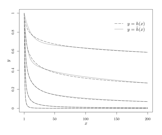
Figure S1: Approximation of $h(x)=x^{-\alpha}$ for $\alpha=0.1,0.25,0.5,1,2$.

S.5 Additional Results of the rfMRI Data Analysis

We illustrate the node degrees of marginal connectivity and direct connectivity in Figure S2 (a) and (c), respectively. The top 10 hubs for marginal connectivity and the top 10 hubs for direct connectivity are listed in the following two tables. The coordinates of the center of each hub is given in the Montreal Neurological Institute (MNI) 152 space. The hubs for marginal connectivity with MNI coordinates listed in bold numbers are spatially close to those found in [17] and [29] from studies with multiple subjects. As an illustration, we plot the marginal connectivity and the direct connectivity of a single hub in Figure S2 (b) and (d), respectively, which is ranked No. 1 in degree of marginal connectivity and No. 4 in degree of direct connectivity. This hub has 164 marginally connected nodes and 79 directly connected nodes, where 80% of the directly connected nodes are also marginally connected. It is located in the right inferior parietal cortex, a part of the so-called default mode network [[16]] that is most active during the resting state.

Table S1: Top 10 hubs for marginal connectivity found by hard thresholding

Rank	Location	MNI coordinates	Degree	Direct rank	Direct degree
1	Inferior parietal	48, -72, 24	164	4	79
2	Supramarginal	-60, -36, 36	151	3	82
3	Superior frontal	0, 48, 36	150	6	73
4	Medial orbitofrontal	0, 60, -12	140	20	53
5	Inferior parietal	-36, -72, 36	137	15	61
6	Supramarginal	60, -48, 36	131	1	85
7	Precuneus	0, -72, 48	128	16	58
8	Precuneus	0, -72, 36	125	10	64
9	Rostral middle frontal	-48, 12, 36	121	5	74
10	Inferior parietal	-48, -60, 24	109	37	48

Table S2: Top 10 hubs for direct connectivity found by CLIME

Rank	Location	MNI coordinates	Degree	Marginal rank	Marginal degree
1	Inferior parietal	60, -48, 36	85	6	131
2	Precentral	-48, 0, 48	82	18	98
3	Supramarginal	-60, -36, 36	82	2	151
4	Inferior parietal	48, -72, 24	79	1	164
5	Rostral middle frontal	-48, 12, 36	74	9	121
6	Superior frontal	0, 48, 36	73	3	150
7	Caudal middle frontal	48, 12, 48	68	29	87
8	Middle temporal	60, -60, 12	66	19	96
9	Precuneus	0, -72, 24	65	14	101
10	Precuneus	0, -72, 36	64	8	125

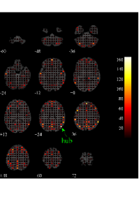
(a)

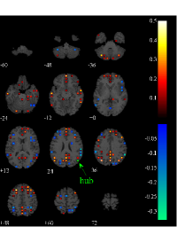
(b)

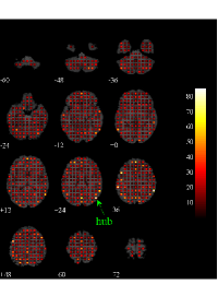
(c)

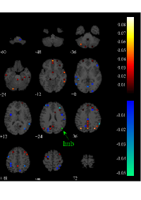
(d)

Figure S2: rfMRI data analysis for brain functional connectivity. (a) Node degrees of marginal connectivity found by hard thresholding. (b) Marginally connected nodes and their estimated correlations to the selected hub. (c) Node degrees of direct connectivity found by CLIME. (d) Directly connected nodes and their estimated partial correlations to the selected hub. The brain is plotted in the Montreal Neurological Institute 152 space with $Z$-coordinates displayed.

References

- [1] {bbook}[author] \bauthor\bsnmAthreya, \bfnmKrishna B.\binitsK. B. and \bauthor\bsnmLahiri, \bfnmSoumendra N.\binitsS. N. (\byear2006). \btitleMeasure theory and probability theory. \bpublisherSpringer, New York. \bmrnumber2247694 \endbibitem
- [2] {barticle}[author] \bauthor\bsnmBai, \bfnmJushan\binitsJ. and \bauthor\bsnmNg, \bfnmSerena\binitsS. (\byear2005). \btitleTests for skewness, kurtosis, and normality for time series data. \bjournalJ. Bus. Econom. Statist. \bvolume23 \bpages49–60. \bdoi10.1198/073500104000000271 \bmrnumber2108691 \endbibitem
- [3] {bbook}[author] \bauthor\bsnmBai, \bfnmZhidong\binitsZ. and \bauthor\bsnmSilverstein, \bfnmJack W.\binitsJ. W. (\byear2010). \btitleSpectral analysis of large dimensional random matrices, \beditionSecond ed. \bpublisherSpringer, New York. \bdoi10.1007/978-1-4419-0661-8 \bmrnumber2567175 \endbibitem
- [4] {barticle}[author] \bauthor\bsnmBai, \bfnmZ. D.\binitsZ. D. and \bauthor\bsnmYin, \bfnmY. Q.\binitsY. Q. (\byear1993). \btitleLimit of the smallest eigenvalue of a large-dimensional sample covariance matrix. \bjournalAnn. Probab. \bvolume21 \bpages1275–1294. \bmrnumber1235416 \endbibitem
- [5] {barticle}[author] \bauthor\bsnmBanerjee, \bfnmOnureena\binitsO., \bauthor\bsnmEl Ghaoui, \bfnmLaurent\binitsL. and \bauthor\bsnmd’Aspremont, \bfnmAlexandre\binitsA. (\byear2008). \btitleModel selection through sparse maximum likelihood estimation for multivariate Gaussian or binary data. \bjournalJ. Mach. Learn. Res. \bvolume9 \bpages485–516. \bmrnumber2417243 \endbibitem
- [6] {barticle}[author] \bauthor\bsnmBasu, \bfnmSumanta\binitsS. and \bauthor\bsnmMichailidis, \bfnmGeorge\binitsG. (\byear2015). \btitleRegularized estimation in sparse high-dimensional time series models. \bjournalAnn. Statist. \bvolume43 \bpages1535–1567. \bdoi10.1214/15-AOS1315 \bmrnumber3357870 \endbibitem
- [7] {barticle}[author] \bauthor\bsnmBenjamini, \bfnmYoav\binitsY. and \bauthor\bsnmYekutieli, \bfnmDaniel\binitsD. (\byear2001). \btitleThe control of the false discovery rate in multiple testing under dependency. \bjournalAnn. Statist. \bvolume29 \bpages1165–1188. \bdoi10.1214/aos/1013699998 \bmrnumber1869245 \endbibitem
- [8] {barticle}[author] \bauthor\bsnmBhattacharjee, \bfnmMonika\binitsM. and \bauthor\bsnmBose, \bfnmArup\binitsA. (\byear2014). \btitleConsistency of large dimensional sample covariance matrix under weak dependence. \bjournalStat. Methodol. \bvolume20 \bpages11–26. \bdoi10.1016/j.stamet.2013.08.005 \bmrnumber3205718 \endbibitem
- [9] {barticle}[author] \bauthor\bsnmBhattacharjee, \bfnmMonika\binitsM. and \bauthor\bsnmBose, \bfnmArup\binitsA. (\byear2014). \btitleEstimation of autocovariance matrices for infinite dimensional vector linear process. \bjournalJ. Time Series Anal. \bvolume35 \bpages262–281. \bdoi10.1111/jtsa.12063 \bmrnumber3194965 \endbibitem
- [10] {barticle}[author] \bauthor\bsnmBickel, \bfnmPeter J.\binitsP. J. and \bauthor\bsnmLevina, \bfnmElizaveta\binitsE. (\byear2008). \btitleCovariance regularization by thresholding. \bjournalAnn. Statist. \bvolume36 \bpages2577–2604. \bdoi10.1214/08-AOS600 \bmrnumber2485008 \endbibitem
- [11] {barticle}[author] \bauthor\bsnmBickel, \bfnmPeter J.\binitsP. J. and \bauthor\bsnmLevina, \bfnmElizaveta\binitsE. (\byear2008). \btitleRegularized estimation of large covariance matrices. \bjournalAnn. Statist. \bvolume36 \bpages199–227. \bdoi10.1214/009053607000000758 \bmrnumber2387969 \endbibitem
- [12] {bbook}[author] \bauthor\bsnmBillingsley, \bfnmPatrick\binitsP. (\byear1995). \btitleProbability and measure, \beditionThird ed. \bpublisherJohn Wiley & Sons, Inc., New York. \bmrnumber1324786 \endbibitem
- [13] {barticle}[author] \bauthor\bsnmBochud, \bfnmThierry\binitsT. and \bauthor\bsnmChallet, \bfnmDamien\binitsD. (\byear2007). \btitleOptimal approximations of power laws with exponentials: application to volatility models with long memory. \bjournalQuant. Finance \bvolume7 \bpages585–589. \bdoi10.1080/14697680701278291 \bmrnumber2374605 \endbibitem
- [14] {barticle}[author] \bauthor\bsnmBradley, \bfnmRichard C.\binitsR. C. (\byear2005). \btitleBasic properties of strong mixing conditions. A survey and some open questions. Update of, and a supplement to, the 1986 original. \bjournalProbab. Surv. \bvolume2 \bpages107–144. \bdoi10.1214/154957805100000104 \bmrnumber2178042 \endbibitem
- [15] {bbook}[author] \bauthor\bsnmBrockwell, \bfnmPeter J.\binitsP. J. and \bauthor\bsnmDavis, \bfnmRichard A.\binitsR. A. (\byear1991). \btitleTime series: theory and methods, \beditionSecond ed. \bpublisherSpringer-Verlag, New York. \bdoi10.1007/978-1-4419-0320-4 \bmrnumber1093459 \endbibitem
- [16] {barticle}[author] \bauthor\bsnmBuckner, \bfnmRandy L\binitsR. L., \bauthor\bsnmAndrews-Hanna, \bfnmJessica R\binitsJ. R. and \bauthor\bsnmSchacter, \bfnmDaniel L\binitsD. L. (\byear2008). \btitleThe brain’s default network. \bjournalAnn. N. Y. Acad. Sci. \bvolume1124 \bpages1–38. \endbibitem
- [17] {barticle}[author] \bauthor\bsnmBuckner, \bfnmRandy L\binitsR. L., \bauthor\bsnmSepulcre, \bfnmJorge\binitsJ., \bauthor\bsnmTalukdar, \bfnmTanveer\binitsT., \bauthor\bsnmKrienen, \bfnmFenna M\binitsF. M., \bauthor\bsnmLiu, \bfnmHesheng\binitsH., \bauthor\bsnmHedden, \bfnmTrey\binitsT., \bauthor\bsnmAndrews-Hanna, \bfnmJessica R\binitsJ. R., \bauthor\bsnmSperling, \bfnmReisa A\binitsR. A. and \bauthor\bsnmJohnson, \bfnmKeith A\binitsK. A. (\byear2009). \btitleCortical hubs revealed by intrinsic functional connectivity: mapping, assessment of stability, and relation to Alzheimer’s disease. \bjournalJ. Neurosci. \bvolume29 \bpages1860–1873. \endbibitem
- [18] {barticle}[author] \bauthor\bsnmCai, \bfnmTony\binitsT. and \bauthor\bsnmLiu, \bfnmWeidong\binitsW. (\byear2011). \btitleAdaptive thresholding for sparse covariance matrix estimation. \bjournalJ. Amer. Statist. Assoc. \bvolume106 \bpages672–684. \bdoi10.1198/jasa.2011.tm10560 \bmrnumber2847949 \endbibitem
- [19] {barticle}[author] \bauthor\bsnmCai, \bfnmTony\binitsT., \bauthor\bsnmLiu, \bfnmWeidong\binitsW. and \bauthor\bsnmLuo, \bfnmXi\binitsX. (\byear2011). \btitleA constrained minimization approach to sparse precision matrix estimation. \bjournalJ. Amer. Statist. Assoc. \bvolume106 \bpages594–607. \bdoi10.1198/jasa.2011.tm10155 \bmrnumber2847973 \endbibitem
- [20] {barticle}[author] \bauthor\bsnmCai, \bfnmT. Tony\binitsT. T., \bauthor\bsnmLiu, \bfnmWeidong\binitsW. and \bauthor\bsnmZhou, \bfnmHarrison H.\binitsH. H. (\byear2016). \btitleEstimating sparse precision matrix: optimal rates of convergence and adaptive estimation. \bjournalAnn. Statist. \bvolume44 \bpages455–488. \bdoi10.1214/13-AOS1171 \bmrnumber3476606 \endbibitem
- [21] {barticle}[author] \bauthor\bsnmCai, \bfnmT. Tony\binitsT. T. and \bauthor\bsnmYuan, \bfnmMing\binitsM. (\byear2012). \btitleAdaptive covariance matrix estimation through block thresholding. \bjournalAnn. Statist. \bvolume40 \bpages2014–2042. \bdoi10.1214/12-AOS999 \bmrnumber3059075 \endbibitem
- [22] {barticle}[author] \bauthor\bsnmCai, \bfnmT. Tony\binitsT. T., \bauthor\bsnmZhang, \bfnmCun-Hui\binitsC.-H. and \bauthor\bsnmZhou, \bfnmHarrison H.\binitsH. H. (\byear2010). \btitleOptimal rates of convergence for covariance matrix estimation. \bjournalAnn. Statist. \bvolume38 \bpages2118–2144. \bdoi10.1214/09-AOS752 \bmrnumber2676885 \endbibitem
- [23] {barticle}[author] \bauthor\bsnmCai, \bfnmT. Tony\binitsT. T. and \bauthor\bsnmZhou, \bfnmHarrison H.\binitsH. H. (\byear2012). \btitleOptimal rates of convergence for sparse covariance matrix estimation. \bjournalAnn. Statist. \bvolume40 \bpages2389–2420. \bdoi10.1214/12-AOS998 \bmrnumber3097607 \endbibitem
- [24] {barticle}[author] \bauthor\bsnmCao, \bfnmGuangzhi\binitsG., \bauthor\bsnmBachega, \bfnmLeonardo R.\binitsL. R. and \bauthor\bsnmBouman, \bfnmCharles A.\binitsC. A. (\byear2011). \btitleThe sparse matrix transform for covariance estimation and analysis of high dimensional signals. \bjournalIEEE Trans. Image Process. \bvolume20 \bpages625–640. \bdoi10.1109/TIP.2010.2071390 \bmrnumber2799176 \endbibitem
- [25] {barticle}[author] \bauthor\bsnmChen, \bfnmXiaohui\binitsX., \bauthor\bsnmXu, \bfnmMengyu\binitsM. and \bauthor\bsnmWu, \bfnmWei Biao\binitsW. B. (\byear2013). \btitleCovariance and precision matrix estimation for high-dimensional time series. \bjournalAnn. Statist. \bvolume41 \bpages2994–3021. \bdoi10.1214/13-AOS1182 \bmrnumber3161455 \endbibitem
- [26] {barticle}[author] \bauthor\bsnmChen, \bfnmXiaohui\binitsX., \bauthor\bsnmXu, \bfnmMengyu\binitsM. and \bauthor\bsnmWu, \bfnmWei Biao\binitsW. B. (\byear2016). \btitleRegularized estimation of linear functionals of precision matrices for high-dimensional time series. \bjournalIEEE Transactions on Signal Processing \bvolume64 \bpages6459–6470. \endbibitem
- [27] {barticle}[author] \bauthor\bsnmChlebus, \bfnmEdward\binitsE. (\byear2009). \btitleAn approximate formula for a partial sum of the divergent -series. \bjournalAppl. Math. Lett. \bvolume22 \bpages732–737. \bdoi10.1016/j.aml.2008.07.007 \bmrnumber2514902 \endbibitem
- [28] {barticle}[author] \bauthor\bsnmCiuciu, \bfnmPhilippe\binitsP., \bauthor\bsnmAbry, \bfnmPatrice\binitsP. and \bauthor\bsnmHe, \bfnmBiyu J\binitsB. J. (\byear2014). \btitleInterplay between functional connectivity and scale-free dynamics in intrinsic fMRI networks. \bjournalNeuroImage \bvolume95 \bpages248–263. \endbibitem
- [29] {barticle}[author] \bauthor\bsnmCole, \bfnmMichael W\binitsM. W., \bauthor\bsnmPathak, \bfnmSudhir\binitsS. and \bauthor\bsnmSchneider, \bfnmWalter\binitsW. (\byear2010). \btitleIdentifying the brain’s most globally connected regions. \bjournalNeuroimage \bvolume49 \bpages3132–3148. \endbibitem
- [30] {bbook}[author] \bauthor\bsnmCramér, \bfnmHarald\binitsH. (\byear1946). \btitleMathematical Methods of Statistics. \bpublisherPrinceton University Press, Princeton, N. J. \bmrnumber0016588 \endbibitem
- [31] {barticle}[author] \bauthor\bsnmDemko, \bfnmStephen\binitsS., \bauthor\bsnmMoss, \bfnmWilliam F.\binitsW. F. and \bauthor\bsnmSmith, \bfnmPhilip W.\binitsP. W. (\byear1984). \btitleDecay rates for inverses of band matrices. \bjournalMath. Comp. \bvolume43 \bpages491–499. \bdoi10.2307/2008290 \bmrnumber758197 \endbibitem
- [32] {barticle}[author] \bauthor\bsnmEl Karoui, \bfnmNoureddine\binitsN. (\byear2008). \btitleOperator norm consistent estimation of large-dimensional sparse covariance matrices. \bjournalAnn. Statist. \bvolume36 \bpages2717–2756. \bdoi10.1214/07-AOS559 \bmrnumber2485011 \endbibitem
- [33] {barticle}[author] \bauthor\bsnmErdős, \bfnmLászló\binitsL., \bauthor\bsnmKnowles, \bfnmAntti\binitsA., \bauthor\bsnmYau, \bfnmHorng-Tzer\binitsH.-T. and \bauthor\bsnmYin, \bfnmJun\binitsJ. (\byear2013). \btitleDelocalization and diffusion profile for random band matrices. \bjournalComm. Math. Phys. \bvolume323 \bpages367–416. \bdoi10.1007/s00220-013-1773-3 \bmrnumber3085669 \endbibitem
- [34] {barticle}[author] \bauthor\bsnmFang, \bfnmYixin\binitsY., \bauthor\bsnmWang, \bfnmBinhuan\binitsB. and \bauthor\bsnmFeng, \bfnmYang\binitsY. (\byear2016). \btitleTuning-parameter selection in regularized estimations of large covariance matrices. \bjournalJ. Stat. Comput. Simul. \bvolume86 \bpages494–509. \bdoi10.1080/00949655.2015.1017823 \bmrnumber3421741 \endbibitem
- [35] {bbook}[author] \bauthor\bsnmFomin, \bfnmVladimir\binitsV. (\byear1999). \btitleOptimal filtering. Vol. II: Spatio-temporal fields. \bpublisherKluwer Academic Publishers, Dordrecht. \bdoi10.1007/978-94-011-4691-3 \bmrnumber1707320 \endbibitem
- [36] {bbook}[author] \bauthor\bsnmFoucart, \bfnmSimon\binitsS. and \bauthor\bsnmRauhut, \bfnmHolger\binitsH. (\byear2013). \btitleA mathematical introduction to compressive sensing. \bpublisherBirkhäuser/Springer, New York. \bdoi10.1007/978-0-8176-4948-7 \bmrnumber3100033 \endbibitem
- [37] {barticle}[author] \bauthor\bsnmFriedman, \bfnmJerome\binitsJ., \bauthor\bsnmHastie, \bfnmTrevor\binitsT. and \bauthor\bsnmTibshirani, \bfnmRobert\binitsR. (\byear2008). \btitleSparse inverse covariance estimation with the graphical lasso. \bjournalBiostatistics \bvolume9 \bpages432–441. \endbibitem
- [38] {barticle}[author] \bauthor\bsnmGeweke, \bfnmJohn\binitsJ. and \bauthor\bsnmPorter-Hudak, \bfnmSusan\binitsS. (\byear1983). \btitleThe estimation and application of long memory time series models. \bjournalJ. Time Ser. Anal. \bvolume4 \bpages221–238. \bdoi10.1111/j.1467-9892.1983.tb00371.x \bmrnumber738585 \endbibitem
- [39] {bbook}[author] \bauthor\bsnmGolub, \bfnmGene H.\binitsG. H. and \bauthor\bsnmVan Loan, \bfnmCharles F.\binitsC. F. (\byear1996). \btitleMatrix computations, \beditionThird ed. \bpublisherJohns Hopkins University Press, Baltimore, MD. \bmrnumber1417720 \endbibitem
- [40] {barticle}[author] \bauthor\bsnmGranger, \bfnmC. W. J.\binitsC. W. J. and \bauthor\bsnmJoyeux, \bfnmRoselyne\binitsR. (\byear1980). \btitleAn introduction to long-memory time series models and fractional differencing. \bjournalJ. Time Ser. Anal. \bvolume1 \bpages15–29. \bdoi10.1111/j.1467-9892.1980.tb00297.x \bmrnumber605572 \endbibitem
- [41] {barticle}[author] \bauthor\bsnmHarrison, \bfnmL\binitsL., \bauthor\bsnmPenny, \bfnmWilliam D\binitsW. D. and \bauthor\bsnmFriston, \bfnmKarl\binitsK. (\byear2003). \btitleMultivariate autoregressive modeling of fMRI time series. \bjournalNeuroimage \bvolume19 \bpages1477–1491. \endbibitem
- [42] {bbook}[author] \bauthor\bsnmHastie, \bfnmTrevor\binitsT., \bauthor\bsnmTibshirani, \bfnmRobert\binitsR. and \bauthor\bsnmFriedman, \bfnmJerome\binitsJ. (\byear2009). \btitleThe elements of statistical learning, \beditionsecond ed. \bseriesSpringer Series in Statistics. \bpublisherSpringer, New York \bnoteData mining, inference, and prediction. \bdoi10.1007/978-0-387-84858-7 \bmrnumber2722294 \endbibitem
- [43] {barticle}[author] \bauthor\bsnmHe, \bfnmBiyu J\binitsB. J. (\byear2011). \btitleScale-free properties of the functional magnetic resonance imaging signal during rest and task. \bjournalJournal of Neuroscience \bvolume31 \bpages13786–13795. \endbibitem
- [44] {barticle}[author] \bauthor\bsnmHinich, \bfnmMelvin J.\binitsM. J. (\byear1982). \btitleTesting for Gaussianity and linearity of a stationary time series. \bjournalJ. Time Ser. Anal. \bvolume3 \bpages169–176. \bdoi10.1111/j.1467-9892.1982.tb00339.x \bmrnumber695228 \endbibitem
- [45] {barticle}[author] \bauthor\bsnmHosking, \bfnmJ. R. M.\binitsJ. R. M. (\byear1981). \btitleFractional differencing. \bjournalBiometrika \bvolume68 \bpages165–176. \bdoi10.1093/biomet/68.1.165 \bmrnumber614953 \endbibitem
- [46] {barticle}[author] \bauthor\bsnmHsieh, \bfnmCho-Jui\binitsC.-J., \bauthor\bsnmSustik, \bfnmMátyás A.\binitsM. A., \bauthor\bsnmDhillon, \bfnmInderjit S.\binitsI. S. and \bauthor\bsnmRavikumar, \bfnmPradeep\binitsP. (\byear2014). \btitleQUIC: quadratic approximation for sparse inverse covariance estimation. \bjournalJ. Mach. Learn. Res. \bvolume15 \bpages2911–2947. \bmrnumber3277149 \endbibitem
- [47] {barticle}[author] \bauthor\bsnmHu, \bfnmTien-Chung\binitsT.-C., \bauthor\bsnmRosalsky, \bfnmAndrew\binitsA. and \bauthor\bsnmVolodin, \bfnmAndrei\binitsA. (\byear2008). \btitleOn convergence properties of sums of dependent random variables under second moment and covariance restrictions. \bjournalStatist. Probab. Lett. \bvolume78 \bpages1999–2005. \bdoi10.1016/j.spl.2008.01.073 \bmrnumber2458009 \endbibitem
- [48] {barticle}[author] \bauthor\bsnmHuang, \bfnmJianhua Z.\binitsJ. Z., \bauthor\bsnmLiu, \bfnmNaiping\binitsN., \bauthor\bsnmPourahmadi, \bfnmMohsen\binitsM. and \bauthor\bsnmLiu, \bfnmLinxu\binitsL. (\byear2006). \btitleCovariance matrix selection and estimation via penalised normal likelihood. \bjournalBiometrika \bvolume93 \bpages85–98. \bdoi10.1093/biomet/93.1.85 \bmrnumber2277742 \endbibitem
- [49] {barticle}[author] \bauthor\bsnmJiang, \bfnmTiefeng\binitsT. (\byear2004). \btitleThe limiting distributions of eigenvalues of sample correlation matrices. \bjournalSankhyā \bvolume66 \bpages35–48. \bmrnumber2082906 \endbibitem
- [50] {barticle}[author] \bauthor\bsnmLam, \bfnmClifford\binitsC. and \bauthor\bsnmFan, \bfnmJianqing\binitsJ. (\byear2009). \btitleSparsistency and rates of convergence in large covariance matrix estimation. \bjournalAnn. Statist. \bvolume37 \bpages4254–4278. \bdoi10.1214/09-AOS720 \bmrnumber2572459 \endbibitem
- [51] {barticle}[author] \bauthor\bsnmLi, \bfnmXingguo\binitsX., \bauthor\bsnmZhao, \bfnmTuo\binitsT., \bauthor\bsnmYuan, \bfnmXiaoming\binitsX. and \bauthor\bsnmLiu, \bfnmHan\binitsH. (\byear2015). \btitleThe flare package for high dimensional linear regression and precision matrix estimation in R. \bjournalJ. Mach. Learn. Res. \bvolume16 \bpages553–557. \bmrnumber3335796 \endbibitem
- [52] {barticle}[author] \bauthor\bsnmLiu, \bfnmHaoyang\binitsH., \bauthor\bsnmAue, \bfnmAlexander\binitsA. and \bauthor\bsnmPaul, \bfnmDebashis\binitsD. (\byear2015). \btitleOn the Marčenko-Pastur law for linear time series. \bjournalAnn. Statist. \bvolume43 \bpages675–712. \bdoi10.1214/14-AOS1294 \bmrnumber3319140 \endbibitem
- [53] {barticle}[author] \bauthor\bsnmLiu, \bfnmHan\binitsH., \bauthor\bsnmLafferty, \bfnmJohn\binitsJ. and \bauthor\bsnmWasserman, \bfnmLarry\binitsL. (\byear2009). \btitleThe nonparanormal: semiparametric estimation of high dimensional undirected graphs. \bjournalJ. Mach. Learn. Res. \bvolume10 \bpages2295–2328. \bmrnumber2563983 \endbibitem
- [54] {barticle}[author] \bauthor\bsnmMandelbrot, \bfnmBenoit B.\binitsB. B. and \bauthor\bsnmVan Ness, \bfnmJohn W.\binitsJ. W. (\byear1968). \btitleFractional Brownian motions, fractional noises and applications. \bjournalSIAM Rev. \bvolume10 \bpages422–437. \bdoi10.1137/1010093 \bmrnumber0242239 \endbibitem
- [55] {bbook}[author] \bauthor\bsnmManolakis, \bfnmDimitris G\binitsD. G., \bauthor\bsnmIngle, \bfnmVinay K\binitsV. K. and \bauthor\bsnmKogon, \bfnmStephen M\binitsS. M. (\byear2005). \btitleStatistical and adaptive signal processing: spectral estimation, signal modeling, adaptive filtering, and array processing \bvolume46. \bpublisherArtech House, Norwood, MA. \endbibitem
- [56] {barticle}[author] \bauthor\bsnmMeinshausen, \bfnmNicolai\binitsN. and \bauthor\bsnmBühlmann, \bfnmPeter\binitsP. (\byear2006). \btitleHigh-dimensional graphs and variable selection with the lasso. \bjournalAnn. Statist. \bvolume34 \bpages1436–1462. \bdoi10.1214/009053606000000281 \bmrnumber2278363 \endbibitem
- [57] {bbook}[author] \bauthor\bsnmPalma, \bfnmWilfredo\binitsW. (\byear2007). \btitleLong-memory time series: Theory and methods. \bpublisherWiley-Interscience, Hoboken, NJ. \bdoi10.1002/9780470131466 \bmrnumber2297359 \endbibitem
- [58] {barticle}[author] \bauthor\bsnmPower, \bfnmJonathan D\binitsJ. D., \bauthor\bsnmCohen, \bfnmAlexander L\binitsA. L., \bauthor\bsnmNelson, \bfnmSteven M\binitsS. M., \bauthor\bsnmWig, \bfnmGagan S\binitsG. S., \bauthor\bsnmBarnes, \bfnmKelly Anne\binitsK. A., \bauthor\bsnmChurch, \bfnmJessica A\binitsJ. A., \bauthor\bsnmVogel, \bfnmAlecia C\binitsA. C., \bauthor\bsnmLaumann, \bfnmTimothy O\binitsT. O., \bauthor\bsnmMiezin, \bfnmFran M\binitsF. M., \bauthor\bsnmSchlaggar, \bfnmBradley L\binitsB. L. \betalet al. (\byear2011). \btitleFunctional network organization of the human brain. \bjournalNeuron \bvolume72 \bpages665–678. \endbibitem
- [59] {barticle}[author] \bauthor\bsnmPriestley, \bfnmM. B.\binitsM. B. and \bauthor\bsnmSubba Rao, \bfnmT.\binitsT. (\byear1969). \btitleA test for non-stationarity of time-series. \bjournalJ. Roy. Statist. Soc. Ser. B \bvolume31 \bpages140–149. \bmrnumber0269062 \endbibitem
- [60] {barticle}[author] \bauthor\bsnmRacine, \bfnmJeff\binitsJ. (\byear2000). \btitleConsistent cross-validatory model-selection for dependent data: hv-block cross-validation. \bjournalJournal of Econometrics \bvolume99 \bpages39–61. \endbibitem
- [61] {barticle}[author] \bauthor\bsnmRavikumar, \bfnmPradeep\binitsP., \bauthor\bsnmWainwright, \bfnmMartin J.\binitsM. J., \bauthor\bsnmRaskutti, \bfnmGarvesh\binitsG. and \bauthor\bsnmYu, \bfnmBin\binitsB. (\byear2011). \btitleHigh-dimensional covariance estimation by minimizing -penalized log-determinant divergence. \bjournalElectron. J. Stat. \bvolume5 \bpages935–980. \bdoi10.1214/11-EJS631 \bmrnumber2836766 \endbibitem
- [62] {barticle}[author] \bauthor\bsnmRothman, \bfnmAdam J.\binitsA. J., \bauthor\bsnmBickel, \bfnmPeter J.\binitsP. J., \bauthor\bsnmLevina, \bfnmElizaveta\binitsE. and \bauthor\bsnmZhu, \bfnmJi\binitsJ. (\byear2008). \btitleSparse permutation invariant covariance estimation. \bjournalElectron. J. Stat. \bvolume2 \bpages494–515. \bdoi10.1214/08-EJS176 \bmrnumber2417391 \endbibitem
- [63] {barticle}[author] \bauthor\bsnmRothman, \bfnmAdam J.\binitsA. J., \bauthor\bsnmLevina, \bfnmElizaveta\binitsE. and \bauthor\bsnmZhu, \bfnmJi\binitsJ. (\byear2009). \btitleGeneralized thresholding of large covariance matrices. \bjournalJ. Amer. Statist. Assoc. \bvolume104 \bpages177–186. \bdoi10.1198/jasa.2009.0101 \bmrnumber2504372 \endbibitem
- [64] {barticle}[author] \bauthor\bsnmRothman, \bfnmAdam J.\binitsA. J., \bauthor\bsnmLevina, \bfnmElizaveta\binitsE. and \bauthor\bsnmZhu, \bfnmJi\binitsJ. (\byear2010). \btitleA new approach to Cholesky-based covariance regularization in high dimensions. \bjournalBiometrika \bvolume97 \bpages539–550. \bdoi10.1093/biomet/asq022 \bmrnumber2672482 \endbibitem
- [65] {barticle}[author] \bauthor\bsnmRudelson, \bfnmMark\binitsM. and \bauthor\bsnmVershynin, \bfnmRoman\binitsR. (\byear2013). \btitleHanson-Wright inequality and sub-Gaussian concentration. \bjournalElectron. Commun. Probab. \bvolume18 \bpagesno. 82, 9. \bdoi10.1214/ECP.v18-2865 \bmrnumber3125258 \endbibitem
- [66] {barticle}[author] \bauthor\bsnmRyali, \bfnmSrikanth\binitsS., \bauthor\bsnmChen, \bfnmTianwen\binitsT., \bauthor\bsnmSupekar, \bfnmKaustubh\binitsK. and \bauthor\bsnmMenon, \bfnmVinod\binitsV. (\byear2012). \btitleEstimation of functional connectivity in fMRI data using stability selection-based sparse partial correlation with elastic net penalty. \bjournalNeuroImage \bvolume59 \bpages3852–3861. \endbibitem
- [67] {barticle}[author] \bauthor\bsnmSripada, \bfnmChandra\binitsC., \bauthor\bsnmAngstadt, \bfnmMichael\binitsM., \bauthor\bsnmKessler, \bfnmDaniel\binitsD., \bauthor\bsnmPhan, \bfnmK Luan\binitsK. L., \bauthor\bsnmLiberzon, \bfnmIsrael\binitsI., \bauthor\bsnmEvans, \bfnmGary W\binitsG. W., \bauthor\bsnmWelsh, \bfnmRobert C\binitsR. C., \bauthor\bsnmKim, \bfnmPilyoung\binitsP. and \bauthor\bsnmSwain, \bfnmJames E\binitsJ. E. (\byear2014). \btitleVolitional regulation of emotions produces distributed alterations in connectivity between visual, attention control, and default networks. \bjournalNeuroImage \bvolume89 \bpages110–121. \endbibitem
- [68] {bincollection}[author] \bauthor\bsnmSyed, \bfnmMujahid N.\binitsM. N., \bauthor\bsnmPrincipe, \bfnmJose C.\binitsJ. C. and \bauthor\bsnmPardalos, \bfnmPanos M.\binitsP. M. (\byear2012). \btitleCorrentropy in data classification. In \bbooktitleDynamics of information systems: mathematical foundations \bpages81–117. \bpublisherSpringer, New York. \bdoi10.1007/978-1-4614-3906-6_5 \bmrnumber3067311 \endbibitem
- [69] {barticle}[author] \bauthor\bsnmTagliazucchi, \bfnmEnzo\binitsE., \bauthor\bparticlevon \bsnmWegner, \bfnmFrederic\binitsF., \bauthor\bsnmMorzelewski, \bfnmAstrid\binitsA., \bauthor\bsnmBrodbeck, \bfnmVerena\binitsV., \bauthor\bsnmJahnke, \bfnmKolja\binitsK. and \bauthor\bsnmLaufs, \bfnmHelmut\binitsH. (\byear2013). \btitleBreakdown of long-range temporal dependence in default mode and attention networks during deep sleep. \bjournalProc. Natl. Acad. Sci. \bvolume110 \bpages15419–15424. \endbibitem
- [70] {bincollection}[author] \bauthor\bsnmTaqqu, \bfnmMurad S.\binitsM. S. (\byear2003). \btitleFractional Brownian motion and long-range dependence. In \bbooktitleTheory and applications of long-range dependence \bpages5–38. \bpublisherBirkhäuser Boston, Boston, MA. \bmrnumber1956042 \endbibitem
- [71] {barticle}[author] \bauthor\bparticlevan de \bsnmGeer, \bfnmSara\binitsS., \bauthor\bsnmBühlmann, \bfnmPeter\binitsP., \bauthor\bsnmRitov, \bfnmYa’acov\binitsY. and \bauthor\bsnmDezeure, \bfnmRuben\binitsR. (\byear2014). \btitleOn asymptotically optimal confidence regions and tests for high-dimensional models. \bjournalAnn. Statist. \bvolume42 \bpages1166–1202. \bdoi10.1214/14-AOS1221 \bmrnumber3224285 \endbibitem
- [72] {bincollection}[author] \bauthor\bsnmVershynin, \bfnmRoman\binitsR. (\byear2012). \btitleIntroduction to the non-asymptotic analysis of random matrices. In \bbooktitleCompressed sensing \bpages210–268. \bpublisherCambridge Univ. Press, Cambridge. \bmrnumber2963170 \endbibitem
- [73] {bbook}[author] \bauthor\bsnmVershynin, \bfnmRoman\binitsR. (\byear2016). \btitleFour lectures on probabilistic methods for data science. \bseries2016 PCMI Summer School. \bpublisherAMS. \bnotearXiv:1612.06661. \endbibitem
- [74] {barticle}[author] \bauthor\bsnmWu, \bfnmWei Biao\binitsW. B. (\byear2005). \btitleNonlinear system theory: another look at dependence. \bjournalProc. Natl. Acad. Sci. \bvolume102 \bpages14150–14154 (electronic). \bdoi10.1073/pnas.0506715102 \bmrnumber2172215 \endbibitem
- [75] {barticle}[author] \bauthor\bsnmWu, \bfnmWei Biao\binitsW. B. and \bauthor\bsnmPourahmadi, \bfnmMohsen\binitsM. (\byear2009). \btitleBanding sample autocovariance matrices of stationary processes. \bjournalStatist. Sinica \bvolume19 \bpages1755–1768. \bmrnumber2589209 \endbibitem
- [76] {barticle}[author] \bauthor\bsnmWu, \bfnmWei-Biao\binitsW.-B. and \bauthor\bsnmWu, \bfnmYing Nian\binitsY. N. (\byear2016). \btitlePerformance bounds for parameter estimates of high-dimensional linear models with correlated errors. \bjournalElectron. J. Stat. \bvolume10 \bpages352–379. \bdoi10.1214/16-EJS1108 \bmrnumber3466186 \endbibitem
- [77] {barticle}[author] \bauthor\bsnmYuan, \bfnmMing\binitsM. (\byear2010). \btitleHigh dimensional inverse covariance matrix estimation via linear programming. \bjournalJ. Mach. Learn. Res. \bvolume11 \bpages2261–2286. \bmrnumber2719856 \endbibitem
- [78] {barticle}[author] \bauthor\bsnmYuan, \bfnmMing\binitsM. and \bauthor\bsnmLin, \bfnmYi\binitsY. (\byear2007). \btitleModel selection and estimation in the Gaussian graphical model. \bjournalBiometrika \bvolume94 \bpages19–35. \bdoi10.1093/biomet/asm018 \bmrnumber2367824 \endbibitem
- [79] {barticle}[author] \bauthor\bsnmZhao, \bfnmTuo\binitsT., \bauthor\bsnmLiu, \bfnmHan\binitsH., \bauthor\bsnmRoeder, \bfnmKathryn\binitsK., \bauthor\bsnmLafferty, \bfnmJohn\binitsJ. and \bauthor\bsnmWasserman, \bfnmLarry\binitsL. (\byear2012). \btitleThe huge package for high-dimensional undirected graph estimation in R. \bjournalJ. Mach. Learn. Res. \bvolume13 \bpages1059–1062. \bmrnumber2930633 \endbibitem
- [80] {barticle}[author] \bauthor\bsnmZhou, \bfnmShuheng\binitsS. (\byear2014). \btitleGemini: graph estimation with matrix variate normal instances. \bjournalAnn. Statist. \bvolume42 \bpages532–562. \bdoi10.1214/13-AOS1187 \bmrnumber3210978 \endbibitem