ON REDUCED ARAKELOV DIVISORS OF REAL QUADRATIC FIELDS

Abstract.

We generalize the concept of reduced Arakelov divisors and define $C$-reduced divisors for a given number $C\geq 1$. These $C$-reduced divisors have remarkable properties which are similar to the properties of reduced ones. In this paper, we describe an algorithm to test whether an Arakelov divisor of a real quadratic field $F$ is $C$-reduced in time polynomial in $\log|\Delta_{F}|$ with $\Delta_{F}$ the discriminant of $F$. Moreover, we give an example of a cubic field for which our algorithm does not work.

1. Introduction

The idea of infrastructure of real quadratic fields of Shanks in [11] was modified and extended by Lenstra [5], Schoof [9] and Buchmann and Williams [2] to certain number fields. Finally, it was generalized to arbitrary number fields by Buchmann [1]. In 2008, Schoof [10] gave the first description of infrastructure in terms of reduced Arakelov divisors and the Arakelov class group $\operatorname{Pic}^{0}_{F}$ of a general number field $F$. Reduced Arakelov divisors can be used for computing $\operatorname{Pic}^{0}_{F}$. They form a finite and regularly distributed set in this topological group [10, Propostion 7.2, Theorem 7.4 and 7.7]. Computing $\operatorname{Pic}^{0}_{F}$ is of interest because knowing this group is equivalent to knowing the class group and the unit group of $F$ (see [6] and [10]).

Schoof proposed two algorithms which run in polynomial time in $\log{|\Delta_{F}|}$ with $\Delta_{F}$ the discriminant of $F$ [10, Algorithm 10.3]: the testing algorithm to check whether a given Arakelov divisor $D$ is reduced, and the reduction algorithm to compute a reduced Arakelov divisor that is close to a given divisor $D$ in $\operatorname{Pic}^{0}_{F}$. However, the reduction algorithm requires finding a shortest vector of the lattice associated to the Arakelov divisor, while finding a reasonably short vector using the LLL algorithm is much faster and easier than finding a shortest vector. This leads to modifications and generalizations of the definition of reduced Arakelov divisors.

One of the generalizations, which we call $C$-reduced Arakelov divisors, comes from the reduction algorithm of Schoof [10, Algorithm 10.3]. With this definition, $C$-reduced Arakelov divisors are reduced in the usual sense when $C=1$, and Arakelov divisors that are reduced in the usual sense are $C$-reduced with $C=\sqrt{n}$ (see [10]). $C$-reduced divisors still form a finite and regularly distributed set in $\operatorname{Pic}^{0}_{F}$, just like the reduced divisors.

This modification, however, has a drawback, since for general number fields it is not known how to test whether a given divisor is $C$-reduced. Currently, we have a testing algorithm to do this only for real quadratic fields, in time polynomial in $\log{\left(|\Delta_{F}|\right)}$. It is the main result of this paper, presented in Section 4.

In Section 2, we discuss $C$-reduced Arakelov divisors in an arbitrary number field. Section 3 is devoted to the properties of $C$-reduced fractional ideals of real quadratic fields. An example of real cubic fields in which the testing algorithm is no longer efficient is given in Section 5.

2. $C$-reduced Arakelov divisors

In this section, we introduce $C$-reduced Arakelov divisors of number fields.

Let $F$ be a number field of degree $n$ and $r_{1},r_{2}$ the numbers of real and complex infinite primes (or infinite places) of $F$, respectively. Let

$$F_{\mathbb{R}}:=F\otimes_{\mathbb{Q}}\mathbb{R}\simeq\prod_{\sigma\text{ real}}\mathbb{R}\times\prod_{\sigma\text{ complex}}\mathbb{C}.$$

Here $\sigma$’s are the infinite primes of $F$. Then $F_{\mathbb{R}}$ is an étale $\mathbb{R}$-algebra with the canonical Euclidean structure given by the scalar product
$\hskip 85.35826pt\langle u,v\rangle:=\operatorname{Tr}(u\overline{v})$ for $u=(u_{\sigma})_{\sigma},v=(v_{\sigma})_{\sigma}\in F_{\mathbb{R}}$.
In particular, in terms of coordinates, we have

$$\|u\|^{2}=\operatorname{Tr}(u\overline{u})=\sum_{\sigma\text{ real}}|u_{\sigma}|^{2}+2\sum_{\sigma\text{ complex}}|u_{\sigma}|^{2},\text{ for any }u=(u_{\sigma})_{\sigma}\in F_{\mathbb{R}}.$$

The norm of an element $u=(u_{\sigma})_{\sigma}$ of $F_{\mathbb{R}}$ is defined by

$$N(u):=\prod_{\sigma\text{ real}}u_{\sigma}\cdot\prod_{\sigma\text{ complex}}|u_{\sigma}|^{2}.$$

Definition 2.1.

An Arakelov divisor is a formal finite sum

$$D=\sum\limits_{\mathfrak{p}}n_{\mathfrak{p}}\mathfrak{p}+\sum_{\sigma}x_{\sigma}\sigma$$

where $\mathfrak{p}$ runs over the nonzero prime ideals in $O_{F}$ and $\sigma$ runs over the infinite primes of $F$, with $n_{\mathfrak{p}}\in\mathbb{Z}$ but $x_{\sigma}\in\mathbb{R}$.

To each divisor $D$ we associate the Hermitian line bundle $(I,u)$ where $I=\prod_{\mathfrak{p}}\mathfrak{p}^{-n_{\mathfrak{p}}}$ is a fractional ideal in $F$ and $u=(e^{-x_{\sigma}})_{\sigma}$ is a vector in $\prod_{\sigma}\mathbb{R}_{>0}\subset F_{\mathbb{R}}$.

There is a natural way to associate an ideal lattice to $D$. Indeed, $I$ is embedded into $F_{\mathbb{R}}$ by the infinite primes $\sigma$. Each element $g$ of $I$ is mapped to the vector $(\sigma(g))_{\sigma}$ in $F_{\mathbb{R}}$. Since the vector $ug:=(u_{\sigma}\sigma(g))_{\sigma}\in F_{\mathbb{R}}$, we can define

$$\|g\|_{D}:=\|ug\|.$$

In terms of coordinates, we have

$$\|g\|_{D}^{2}=\sum_{\sigma\text{ real }}u_{\sigma}^{2}|\sigma(g)|^{2}+2\sum_{\sigma\text{ complex }}|u_{\sigma}|^{2}|\sigma(g)|^{2}.$$

With this metric, $I$ becomes an ideal lattice in $F_{\mathbb{R}}$. We call $I$ the ideal lattice associated to $D$. The vector $u$ has the role of a metric for $I$. Hence we make the following definition.

Definition 2.2.

Let $I$ be a fractional ideal in $F$ and let $u$ be in $F_{\mathbb{R}}^{*}$. The length of an element $g$ of $I$ with respect to the metric $u$ is defined by $\|g\|_{u}:=\|ug\|$.

Definition 2.3.

Let $I$ be a fractional ideal. Then 1 is called primitive in $I$ if $1$ belongs to $I$ and it is not divisible by any integer $\geq 2$.

Definition 2.4.

Let $C\geq 1$. A fractional ideal $I$ is called $C$-reduced if:

• $1$ is primitive in $I$.

• There exists a metric $u\in\prod_{\sigma}\mathbb{R}_{>0}$ such that$\|1\|_{u}\leq C\|g\|_{u}$ for all $g\in I\backslash\{0\}$.

Remark 2.5.

The second condition of Definition 2.4 is equivalent to saying that there exists a metric $u$ such that with respect to this metric, the vector $1$ scaled by the scalar $C$ is a shortest vector in the lattice $I$.

Definition 2.6.

Let $I$ be a fractional ideal in $F$. The Arakelov divisor $d(I)$ is defined to be associated with the Hermitian line bundle $(I,u)$ where $u=(u_{\sigma})_{\sigma}$ with $u_{\sigma}=N(I)^{-1/n}$ for all $\sigma$.

Definition 2.7.

An Arakelov divisor $D$ is called $C$-reduced if it has the form $D=d(I)$ for some $C$-reduced fractional ideal $I$.

Now we prove the following lemma.

Lemma 2.8.

Let $I$ be a fractional ideal. If $I$ is $C$-reduced then the inverse $I^{-1}$ of $I$ is an integral ideal and its norm is at most $C^{n}\partial_{F}$ where $\partial_{F}=(2/\pi)^{r_{2}}\sqrt{|\Delta_{F}|}$.

Proof.

Since $1\in I$, we have $I^{-1}\subset O_{F}$. Then $L=N(I)^{-1/n}I$ is a lattice of covolume $\sqrt{|\Delta_{F}|}$ [10, Section 4]. Consider the symmetric, convex and bounded subset of $F_{\mathbb{R}}$,

$$S=\{(x_{\sigma})_{\sigma}:|x_{\sigma}|<\partial_{F}^{1/n}\text{ for all }\sigma\}.$$

For real $\sigma$, the segment $|x_{\sigma}|<\partial_{F}^{1/n}$ in $\mathbb{R}$ has length $2\cdot\partial_{F}^{1/n}$. For complex $\sigma$, the disc $|x_{\sigma}|<\partial_{F}^{1/n}$ in $\mathbb{C}$ has area $2\pi(\partial_{F}^{1/n})^{2}$. Thus,

$$\operatorname{vol}(S)=(2\partial_{F}^{1/n})^{r_{1}}\cdot(2\pi(\partial_{F}^{1/n})^{2})^{r_{2}}=2^{r_{1}}(2\pi)^{r_{2}}\partial_{F}=2^{n}\operatorname{covol}(L).$$

By Minkowski’s theorem, there is a nonzero element $f\in I$ such that

$$N(I)^{-1/n}|\sigma(f)|\leq\partial_{F}^{1/n}\text{ for all }\sigma.$$

Since $I$ is $C$-reduced, there exists a metric $u$ such that $\|1\|_{u}\leq C\|f\|_{u}$. This implies that $\|u\|\leq C\|u\|\max_{\sigma}|\sigma(f)|\leq C\|u\|\partial_{F}^{1/n}N(I)^{1/n}$. Hence $N(I^{-1})\leq C^{n}\partial_{F}$.

∎

Remark 2.9.

In this paper, given a fractional ideal $I$, we assume that it is represented by a matrix with rational entries as in [7, Section 4] and [6, Section 2]. Without loss of generality, we can also assume that the length of the input is polynomial in $\log|\Delta_{F}|$.

By Lemma 2.8, to test whether $I$ is $C$-reduced, first we can check that $N(I)^{-1}\leq C^{n}\partial_{F}$. We have the following.

Lemma 2.10.

Testing $N(I)^{-1}\leq C^{n}\partial_{F}$ can be done in time polynomial in $\log|\Delta_{F}|$.

Proof.

Let $M$ be the matrix representation of $I$. Since we know that $N(I)^{-1}=\sqrt{|\Delta_{F}|}/\operatorname{covol}(I)$, it is sufficient to check that

$$|det(M)|=\operatorname{covol}(I)>(\pi/2)^{r_{2}}C^{n}.$$

Recall that the determinant of the matrix $M$ can be computed in time polynomial [8, Section 1]. This reason and Remark 2.9 imply that testing $N(I)^{-1}\leq C^{n}\partial_{F}$ can be done in time polynomial in $\log|\Delta_{F}|$. ∎

Regarding the primitiveness of $1$ in $I$, we have the result below.

Lemma 2.11.

Let $C\geq 1$ and let $I$ be a fractional ideal containing $1$ with $N(I)^{-1}\leq C^{n}\partial_{F}$. Then testing whether or not $1$ is primitive can be done in time polynomial in $\log{|\Delta_{F}|}$.

Proof.

Let $\{c_{1},...,c_{n}\}$ be an LLL-reduced $\mathbb{Z}$-basis of $O_{F}$ and $\{b_{1},...,b_{n}\}$ be an LLL-reduced $\mathbb{Z}$-basis of $I^{-1}$. Since $1\in I$, we obtain $I^{-1}\subset O_{F}$ and so $b_{i}\in O_{F}$ for all $i$. Then for each $i=1,...,n$, there exist the integers $k_{ij}$ with $j=1,...,n$ for which $b_{i}=\sum_{i}k_{ij}c_{j}$. Thus, there is an integer $d$ such that $1/d\in I$ if and only if $I^{-1}\subset dO_{F}$. This is equivalent to $d|k_{ij}$ for all $i,j$. In other words, $d|\gcd(k_{ij},1\leq i,j\leq n)$. In conclusion, $1$ is primitive in $I$ if and only if $\gcd(k_{ij},1\leq i,j\leq n)=1$.

Since $N(I)^{-1}\leq C^{n}\partial_{F}$, an LLL-reduced $\mathbb{Z}$-basis of $I$, the coefficients $k_{ij}$ and $\gcd(k_{ij},1\leq i,j\leq n)$ can be computed in polynomial time in $\log{|\Delta_{F}|}$. In other words, testing the primitiveness of $1$ can be done in time polynomial in $\log{|\Delta_{F}|}$. ∎

By Lemma 2.11, we know how to test the first condition of Definition 2.4. From now on, we only consider the second condition of this definition.

Remark 2.12.

Note that if $u\in\prod_{\sigma}\mathbb{R}_{>0}$ satisfies the second condition of Definition 2.4, then $u^{\prime}=\left(u_{\sigma}/N(u)^{1/n}\right)_{\sigma}\in\prod_{\sigma}\mathbb{R}_{>0}$ still satisfies that condition and $N(u^{\prime})=1$. Therefore, we can always assume that $N(u)=1$ from now on.

Proposition 2.13.

Let $I$ be a fractional ideal and $u$ be a vector satisfying the second condition of Definition 2.4 with $N(u)=1$. Then

$$\|u\|\leq C\sqrt{n}(2/\pi)^{r_{2}/n}\operatorname{covol}(I)^{1/n}.$$

Proof.

Let $L=uI:=\{uf=(u_{\sigma}\cdot\sigma(f))_{\sigma}:f\in I\}\subset F_{\mathbb{R}}$. Then $L$ is a lattice with metric inherited from $F_{\mathbb{R}}$ (see [10]). Since $N(u)=1$, the lattice $L$ has covolume equal to $\operatorname{covol}(I)$ . Consider the symmetric, convex and bounded subset $S$ of $F_{\mathbb{R}}$

$$S=\{(x_{\sigma}):|x_{\sigma}|<(2/\pi)^{r_{2}/n}\operatorname{covol}(I)^{1/n}\text{ for all }\sigma\}.$$

We have

$$\operatorname{vol}(S)=2^{r_{1}}(2\pi)^{r_{2}}(2/\pi)^{r_{2}}\operatorname{covol}(I)=2^{n}\operatorname{covol}(L).$$

By Minkowski’s theorem, there is a nonzero element $f\in I$ such that

$$u_{\sigma}|\sigma(f)|\leq(2/\pi)^{r_{2}/n}\operatorname{covol}(I)^{1/n}\text{ for all }\sigma.$$

So

$$\|uf\|\leq\sqrt{n}(2/\pi)^{r_{2}/n}\operatorname{covol}(I)^{1/n}.$$

Because $u$ satisfies the second condition of Definition 2.4, we have $\|u\|\leq C\|uf\|$. The proposition is then proved. ∎

3. $C$-reduced Arakelov divisors of real quadratic fields

In this part, fix $C\geq 1$ and a real quadratic field $F$ with the discriminant $\Delta_{F}$, we will describe what $C$-reduced ideals look like, and we will investigate their properties.

Here and in the rest of the paper, we often identify an element $g$ of fractional ideals with its image $(\sigma(g))_{\sigma}\in F_{\mathbb{R}}$. Thus, elements of fractional ideals of real quadratic fields have the form $g=(g_{1},g_{2})\in F_{\mathbb{R}}\cong\mathbb{R}^{2}$.

Remark 3.1.

Let $F$ be an imaginary quadratic field and let $I$ be a fractional ideal of $F$. Then an element $g\in I$ can be identified with its image $g\in F_{\mathbb{R}}\cong\mathbb{C}$. The second condition of Definition 2.4 is equivalent to: there exists $u\in\mathbb{R}_{>0}$ such that $|u|\leq C|ug|$ for all $g\in I\backslash\{0\}$. Since $u$ is a positive real number, this is equivalent to that $1/C\leq|g|$ for all $g\in I\backslash\{0\}$. In other words, the shortest vectors of $I$ have length at least $1/C$. In addition, the first vector in an LLL reduced basis of $I$ is also its shortest vector; finding this vector can also be done in polynomial time. This together with Lemma 2.11 shows that whether a given ideal of an imaginary quadratic field is $C$-reduced can be tested easily and in polynomial time. Therefore, in this section, we only consider $C$-reduced ideals of real quadratic fields.

3.1. A geometrical view of reduced ideals in real quadratic cases

We have $F_{\mathbb{R}}\cong\mathbb{R}^{2}$. Let $I$ be a fractional ideal of $F$ and $S_{1}$ be the square centered at the origin of $F_{\mathbb{R}}$ which has a vertex $(1/C,1/C)$. We have the following result.

Proposition 3.2.

The second condition in Definition 2.4 can be restated as follows. There exists an ellipse $E_{4}$, centered at the origin and passing through the vertices of $S_{1}$, whose interior does not contain any nonzero points of the lattice $I$.

Proof.

It is easy to see by writing down the condition $\|u\|\leq C\|uf\|$ in terms of the coordinates of $u$ and $f$. ∎

Proposition 3.3.

If $I$ has some nonzero element in the square $S_{1}$ then the ellipse $E_{4}$ described in Proposition 3.2 does not exist. On the other hand, $E_{4}$ exists when the shortest vectors of $I$ have length at least $\sqrt{2}/C$.

Proof.

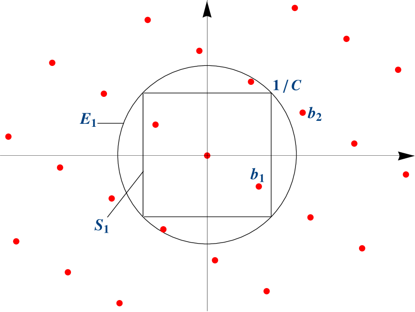
Figure 1. The shortest vectors of $I$ are inside the square $S_{1}$.

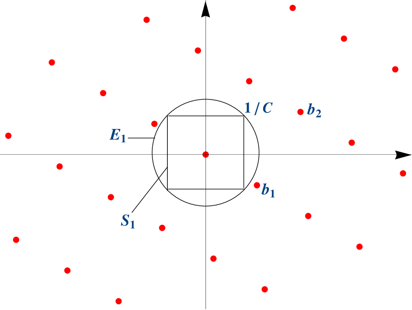
Figure 2. The shortest vectors of $I$ are outside the circle $E_{1}$.

For the first case, we assume that there is a nonzero element $g$ of $I$ in the square $S_{1}$. Since $S_{1}$ is inside $E_{4}$, so is $g$ (see Figure 2). In the second case, we can take for $E_{4}$ the circle $E_{1}$ centered at the origin and of radius $\sqrt{2}/C$. Because the shortest vectors of $I$ are outside $E_{1}$, all the nonzero elements of $I$ are outside $E_{4}$(see Figure 2). ∎

Remark 3.4.

Proposition 3.3 does not show whether the ellipse $E_{4}$ exists or not in case the shortest vectors of $I$ are inside the circle $E_{1}$, and $I$ has no nonzero element in the square $S_{1}$ (see Figure 3). We will discuss this case in the next sections.

Figure 3. The shortest vectors of $I$ are inside $E_{1}$ and $I$ has no nonzero element in $S_{1}$.

3.2. Some properties of $C$-reduced ideals in real quadratic fields

In this section, as mentioned in Remark 3.4, we always assume that $I$ satisfies the conditions $(\star)$ as follows.

$$(\star)\begin{cases}1)\hskip 2.84544pt1\text{ is primitive in }I.\\ 2)\hskip 2.84544ptI\text{ has no nonzero element in the square }\\ S_{1}=\left\{(x_{1},x_{2})\in\mathbb{R}^{2}:|x_{1}|\leq 1/C\text{ and }|x_{2}|\leq 1/C\text{ and }x_{1}^{2}+x_{2}^{2}<2/C^{2}\right\}.\\ 3)\hskip 8.5359pt\text{A shortest vector }f\text{ of }I\text{ has length }1/C<\|f\|<\sqrt{2}/C.\end{cases}$$

Moreover, by Remark 2.12, we can assume that the vector $u$ in Definition 2.4 has the form $u=(\alpha^{-1},\alpha)\in\left(\mathbb{R}_{>0}\right)^{2}\subset F_{\mathbb{R}}$ for some $\alpha\in\mathbb{R}_{>0}$.

Let $\{b_{1}=(b_{1,1},b_{1,2}),b_{2}=(b_{2,1},b_{2,2})\}$ be an LLL-basis of $I$. Then $\|b_{1}\|=\|f\|<\frac{\sqrt{2}}{C}$. We denote by $\{b_{1}^{*},b_{2}^{*}\}$ the Gram-Schmidt orthogonalization of the basis $\{b_{1},b_{2}\}$.

Let

$$G=\{g\in I:\left(g_{1}^{2}-\frac{1}{C^{2}}\right)\left(g_{2}^{2}-\frac{1}{C^{2}}\right)<0\text{ and }\|g\|<\frac{4}{\pi}C\operatorname{covol}(I)\}.$$

We also set

$$G_{1}=\{g\in G:g_{1}^{2}-\frac{1}{C^{2}}<0\}\text{ and }G_{2}=\{g\in G:g_{2}^{2}-\frac{1}{C^{2}}<0\}.$$

So, we obtain $G=G_{1}\cup G_{2}$.
For each $g\in G$, we define

$$B(g):=\left(-\frac{C^{2}g_{1}^{2}-1}{C^{2}g_{2}^{2}-1}\right)^{1/4}.$$

Then denote

(3.1) $$B_{min}=\begin{cases}\frac{1}{2\sqrt{C}}\hskip 85.35826pt\text{ if }&G_{1}=\emptyset\\ \max\left\{B(g):g\in G_{1}\right\}\text{ if }&G_{1}\neq\emptyset.\end{cases}$$

(3.2) $$B_{max}=\begin{cases}2\sqrt{C}\hskip 79.6678pt\text{ if }&G_{2}=\emptyset\\ \min\left\{B(g):g\in G_{2}\right\}\text{ if }&G_{2}\neq\emptyset.\end{cases}$$

Let $G^{\prime}=\{g\in G:B(g)=B_{max}\text{ or }B(g)=B_{min}\}$. Then because of assumption $(\star)$, the vector $b_{1}$ is in $G$. Thus, $G^{\prime}$ is nonempty.

The most important result in this paper is the following proposition.

Proposition 3.5.

The ideal $I$ is $C$-reduced if and only if $B_{min}\leq B_{max}$.

We prove this proposition after proving some results below. First, we establish a property of the ellipses $E_{4}$ described in Section 3.1.

Proposition 3.6.

Assume that $E_{4}:\frac{X_{1}^{2}}{a_{1}^{2}}+\frac{X_{2}^{2}}{a_{2}^{2}}=1$ with $a_{1}>0$ and $a_{2}>0$ is an ellipse satisfying the conclusion of Proposition 3.2. In other words, $E_{4}$ has its center at the origin, passes through the vertices of $S_{1}$ and the interior contains no nonzero points of the lattice $I$. Then:

• The coefficients $a_{1}$ and $a_{2}$ are bounded by $\frac{4}{\pi}C\operatorname{covol}(I)$.

• $E_{4}$ is inside the circle $E_{5}$ of radius $\frac{4}{\pi}C\operatorname{covol}(I)$ centered at the origin.

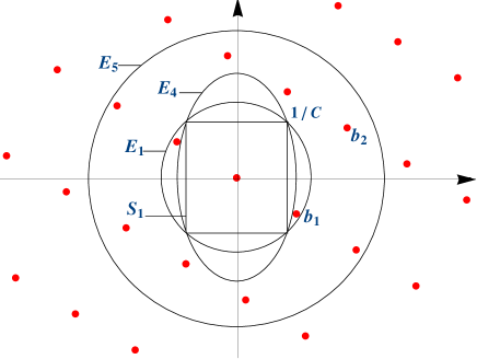
Figure 4. Circle $E_{5}$ and ellipse $E_{4}$.

Proof.

Since $E_{4}$ passes through the vertex $(1/C,1/C)$ of $S_{1}$, its coefficients satisfy $a_{1}>1/C$ and $a_{2}>1/C$ . We also know that $\operatorname{vol}(E_{4})=\pi a_{1}a_{2}$. Hence

$$a_{1}=\frac{\operatorname{vol}(E_{4})}{\pi a_{2}}<\frac{1}{\pi}C\operatorname{vol}(E_{4}).$$

In addition, the ellipse $E_{4}$ is a symmetric, convex and bounded set whose interior contains no nonzero points of the lattice $I$, hence it must have volume less than $2^{2}\operatorname{covol}(I)$ by Minkowski’s theorem. As a consequence,

$$a_{1}<\frac{4}{\pi}C\operatorname{covol}(I).$$

By symmetry, we also have this bound for $a_{2}$. Thus, the first statement of the proposition is obtained. The second one follows from the first. ∎

We have another equivalent condition to Definition 2.4 as follows.

Proposition 3.7.

The second condition of Definition 2.4 is equivalent to the following: there exists a metric $u\in\left(\mathbb{R}_{>0}\right)^{2}$ such that for all $g\in G$, we have $\|1\|_{u}\leq C\|g\|_{u}$.

Proof.

Let $g=(g_{1},g_{2})$ be a nonzero element of $I$. If $\|g\|\geq(4/\pi)C\operatorname{covol}(I)$ then $g$ is outside the circle $E_{5}$. By Proposition 3.6, $g$ is also outside any ellipse $E_{4}$ (see Figure 4). Using this and the equivalent condition of Proposition 3.2, we obtain: a vector $u$ satisfies Definition 2.4 if and only if $\|u\|\leq C\|ug\|$ for all $g\in I\backslash\{0\}$ with $\|g\|<(4/\pi)C\operatorname{covol}(I)$.

On the other hand, if $|g_{1}|\geq 1/C$ and $|g_{2}|\geq 1/C$, then $g$ satisfies $\|u\|\leq C\|ug\|$ for any $u\in\left(\mathbb{R}_{>0}\right)^{2}$. Therefore, it is sufficient to consider the elements $g$ such that $|g_{1}|<1/C$ or $|g_{2}|<1/C$ to show the existence of $u$.

Moreover, $I$ contains no nonzero elements of $S_{1}$, so $g\notin\{(x_{1},x_{2})\in\mathbb{R}^{2}:|x_{1}|\leq 1/C\text{ and }|x_{2}|\leq 1/C\text{ and }x_{1}^{2}+x_{2}^{2}<2/C^{2}\}$.

Combining these conditions, we obtain the conclusion. ∎

The ideal $I$ with properties $(\star)$ mentioned at the beginning of this section has bounded covolume. Explicitly, we obtain the following.

Proposition 3.8.

The covolume of $I$ is bounded by $2/C$.

Proof.

Since $1$ is in $I$, there exist integers $m_{1}$ and $m_{2}$ such that $1=m_{1}b_{1}+m_{2}b_{2}$. If $m_{2}=0$ then $1=m_{1}b_{1}$ so $1/m_{1}=b_{1}\in I$. Because $1$ is primitive in $I$, we must have $m_{1}=\pm 1$. Thus $\|b_{1}\|=\|1\|=\sqrt{2}\geq\sqrt{2}/C$ for any $C\geq 1$. This contradicts the fact that the length of the shortest vectors of $I$ is strictly less than $\sqrt{2}/C$. Hence $m_{2}\neq 0$.

We have $\|b_{2}^{*}\|\leq\frac{1}{|m_{2}|}\|1\|\leq\sqrt{2}$. This leads to the following.

$$\operatorname{covol}(I)=\|b_{1}\|\|b_{2}^{*}\|<\frac{\sqrt{2}}{C}\times\sqrt{2}=\frac{2}{C}.$$

∎

By this proposition and Proposition 3.6, we obtain the corollary below.

Corollary 3.9.

The coefficients $a_{1}$ and $a_{2}$ and the radius of the circle $E_{5}$ in Proposition 3.6 are bounded by $8/\pi$. In addition, the set $G$ is contained in the finite set $\{g\in I:(g_{1}^{2}-1/C^{2})(g_{2}^{2}-1/C^{2})<0\text{ and }\|g\|<8/\pi\}$.

For a real quadratic field, the Proposition 2.13 can be restated as below.

Proposition 3.10.

Assume that $u=(\alpha^{-1},\alpha)\in\left(\mathbb{R}_{>0}\right)^{2}$ satisfies the second condition of Definition 2.4. Then $\|u\|\leq 2\sqrt{C}$ and therefore

$$\frac{1}{2\sqrt{C}}<\alpha<2\sqrt{C}.$$

Proof.

By Proposition 2.13, $\|u\|\leq C\sqrt{2}\operatorname{covol}(I)^{1/2}.$ By Proposition 3.8, we have $\operatorname{covol}(I)<\frac{2}{C}$, so $\|u\|\leq 2\sqrt{C}$. Since $\alpha^{-1}<\|u\|$ and $\alpha<\|u\|$, the conclusion follows. ∎

Proof of Proposition 3.5.

Let $u=(\alpha^{-1},\alpha)\in\left(\mathbb{R}_{>0}\right)^{2}$. Then from $\|1\|_{u}\leq C\|g\|_{u}$, we get

$$\alpha^{4}(C^{2}g_{2}^{2}-1)\geq-(C^{2}g_{1}^{2}-1).$$

Thus $\alpha\geq B(g)$ if $g\in G_{1}$ and $\alpha\leq B(g)$ if $g\in G_{2}$. As $1$ is primitive in $I$, by Proposition 3.7, the ideal $I$ is $C$-reduced if and only if it satisfies the following equivalent conditions:

there exists $u\in\left(\mathbb{R}_{>0}\right)^{2}$ such that $\|1\|_{u}\leq C\|g\|_{u}$ for all $g\in G$,

$$\Leftrightarrow\text{ There exist }\alpha\in\mathbb{R}_{>0}\text{ such that }\begin{cases}\alpha\geq B(g)&\text{ for all }g\in G_{1}\\ \alpha\leq B(g)&\text{ for all }g\in G_{2}\end{cases}$$

$$\Leftrightarrow\text{ There exists }\alpha\in\mathbb{R}_{>0}\text{ such that }\begin{cases}\alpha\geq B_{min}\\ \alpha\leq B_{max}\end{cases}\hskip 73.97733pt$$

$$\Leftrightarrow B_{max}\geq B_{min}.\hskip 241.84842pt$$

The second equivalence comes from Proposition 3.10 and the definition of $B_{min}$ and $B_{max}$. ∎

Proposition 3.5 and 3.7 motivate a further investigation of properties of the sets $G$ and $G^{\prime}$. We first establish a special property of the elements in $G$.

Proposition 3.11.

If $g=s_{1}b_{1}+s_{2}b_{2}\in G$ then $|s_{2}|\leq 1$.

Proof.

Let $g=s_{1}b_{1}+s_{2}b_{2}$ in $G$. As in the proof of Proposition 3.8, we get $\|b_{1}\|<\sqrt{2}/C$ and $\|b_{2}^{*}\|\leq\sqrt{2}$. By the properties of LLL-reduced bases, $\|b_{2}\|\leq\sqrt{2}\|b_{2}^{*}\|\leq 2$. Therefore,

$$\frac{4C\operatorname{covol}(I)}{\pi}=\frac{4C\|b_{1}\|\|b_{2}^{*}\|}{\pi}<\frac{4\sqrt{2}\|b_{2}^{*}\|}{\pi}.$$

Now let $g^{*}$ be a vector of length equal to the distance from $g$ to the 1-dimensional vector space $\mathbb{R}.b_{1}$. In other words, $\|g^{*}\|=d(g,\mathbb{R}.b_{1})=|s_{2}|\|b_{2}^{*}\|$. If $|s_{2}|\geq 2$, then then we would have the following contradiction.

$$\|g\|\geq d(g,\mathbb{R}.b_{1})=\|g^{*}\|\geq 2\|b_{2}^{*}\|>\frac{4\sqrt{2}\|b_{2}^{*}\|}{\pi}>\frac{4}{\pi}C\operatorname{covol}(I).$$

Thus $|s_{2}|\leq 1$. ∎

In the next proposition, we prove that the cardinality of $G$ is bounded by a number that depends only on $C$ but not on $I$ or the number field $F$.

Lemma 3.12.

The number of vectors in $G$ (up to sign) is less than $17C+3$.

Proof.

Let $g\in G$. Then $g=s_{1}b_{1}+s_{2}b_{2}$ for some integers $s_{1},s_{2}$. We have $\|b_{1}\|\geq 1/C$ and $\|g\|<8/\pi$ (by Corollary 3.9). This implies that

$$|s_{1}|\leq\sqrt{2}\left(\frac{3}{2}\right)\frac{\|g\|}{\|b_{1}\|}<\frac{12\sqrt{2}C}{\pi}$$

[7, Section 12]. By Proposition 3.11, we obtain $|s_{2}|\leq 1.$

Consequently, the number of elements in $G$ (up to sign) is at most $3\cdot(\frac{12\sqrt{2}C}{\pi}+1)$, which is less than $17C+3$. ∎

The proposition below gives a property of elements in $G^{\prime}$.

Proposition 3.13.

Let $g=s_{1}b_{1}+b_{2}\in G^{\prime}$. Then:

• $|s_{1}|\leq 2$ or

• $s_{1}\in\{t_{1},t_{2}\}$ for some integers $t_{1}\leq t_{2}$ in the interval $(-1-2C,1+2C)$.

Proof.

It is easy to show that $b_{1}\in G=G_{1}\cup G_{2}$ since $\|b_{1}\|\leq(4/\pi)C\operatorname{covol}(I)$. Here, we only prove the proposition for $b_{1}\in G_{1}$, so $0<b_{11}<1/C$ and $1/C<|b_{12}|<\sqrt{2}/C$. For $b_{1}\in G_{2}$ , it is sufficient to switch $b_{11}$ and $b_{12}$. In the first case, by definition of $B_{min}$, we obtain $B(b_{1})\leq B_{min}$.

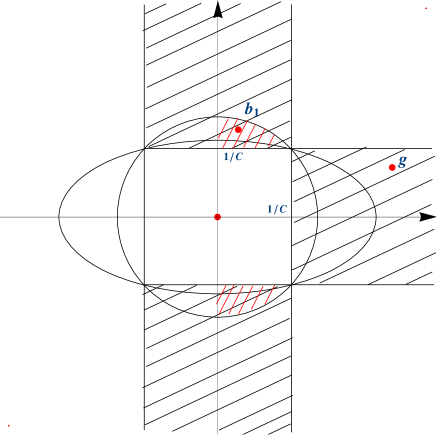
Figure 5. $b_{1}$ is in the doubly-shaded area and $g$ is in the shaded area.

The element $g$ is in $G^{\prime}$, and it belongs to $G_{1}$ or $G_{2}$.

If $g$ is in $G_{1}$ then $0<|g_{1}|<1/C$ and $|g_{2}|>1/C$. Since $g\in G^{\prime}$ and $B(b_{1})\leq B_{min}$, we also have $B(b_{1})\leq B(g)$. If $\|g\|>\sqrt{2}/C$ then $B(b_{1})>B(g)$, contradicting the previous inequality. So, $\|g\|\leq\sqrt{2}/C$. With this in mind and the properties of LLL-reduced bases [7, Section 12], we obtain

$$|s_{1}|\leq\sqrt{2}\left(\frac{3}{2}\right)\frac{\|g\|}{\|b_{1}\|}<\sqrt{2}\left(\frac{3}{2}\right)\left(\frac{\frac{\sqrt{2}}{C}}{\frac{1}{C}}\right)=3\qquad\text{ so }|s_{1}|\leq 2.$$

If $g$ is in $G_{2}$ then $|g_{1}|>1/C$ and $|g_{2}|<1/C$. Since $g=s_{1}b_{1}+b_{2}$ and $|g_{2}|<1/C$, the value of $s_{1}$ is between $\frac{-1/C-b_{22}}{b_{12}}$ and $\frac{1/C-b_{22}}{b_{12}}$. The fact that $0<|b_{12}|<\sqrt{2}/C$ implies that the distance between these numbers

$$\left|\frac{-1/C-b_{22}}{b_{12}}-\frac{1/C-b_{22}}{b_{12}}\right|=\frac{2}{C|b_{12}|}$$

is in the interval $(\sqrt{2},2)$. So, there exist two integers $t_{1}\leq t_{2}$ between these numbers. Moreover, since $1/C<|b_{12}|<\sqrt{2}/C$ and since $|b_{22}|<\|b_{2}\|\leq 2$ (see the proof of Proposition 3.11), one can easily see that

$$\left|\frac{\pm 1/C-b_{22}}{b_{12}}\right|<1+2C.$$

Thus, the bounds for $s_{1}$ are implied, completing the proof.

∎

4. Test algorithm for real quadratic fields

In this section, given $C\geq 1$, we explain an algorithm to test whether a given fractional ideal $I$ is $C$-reduced for a real quadratic field $F$ in time polynomial in $\log|\Delta_{F}|$ with $\Delta_{F}$ the discriminant of $F$.

By Proposition 3.5, if we know $B_{min}$ and $B_{max}$, then we can show the existence of a metric $u=(\alpha^{-1},\alpha)$ in Definition 2.4. In this algorithm, we first find all the possible elements of $G^{\prime}=\{g\in G:B(g)=B_{max}\text{ or }B(g)=B_{min}\}$ and then compute $B_{min}$ and $B_{max}$. Let $\{b_{1},b_{2}\}$ be an LLL-basis of $I$ and $g=s_{1}b_{1}+s_{2}b_{2}\in G^{\prime}$. Then Proposition 3.11 says that $s_{2}=0$ or $s_{2}=\pm 1$. By symmetry, it is sufficient to consider only the case $s_{2}\in\{0,1\}$.

• If $s_{2}=0$ then $g=b_{1}$.

• If $s_{2}=1$ then $g=s_{1}b_{1}+b_{2}$. By Proposition 3.13, there are five possible values for $s_{1}$ in the interval $[-2,2]$ and two possible values $t_{1},t_{2}$ (with $t_{1}\leq t_{2}$) of $s_{1}$ either between $\frac{-1/C-b_{22}}{b_{12}}$ and $\frac{1/C-b_{22}}{b_{12}}$ or between $\frac{-1/C-b_{21}}{b_{11}}$ and $\frac{1/C-b_{21}}{b_{11}}$. This proposition also shows that the coefficients $s_{1}$ have absolute values less than $1+2C$.

Furthermore, by Proposition 3.10, we have $\frac{1}{2\sqrt{C}}<\alpha<2\sqrt{C}$ and so $\frac{1}{16C^{2}}<B(g)^{4}<16C^{2}$ for all $g\in G$. In other words:

$$(\star\star)\begin{cases}\text{If }|g_{2}|<1/C\text{ then }\\ \hskip 28.45274pt|g_{1}|^{2}+16C^{2}|g_{2}|^{2}<16+\frac{1}{C^{2}}\text{ and }|g_{2}|^{2}+16C^{2}|g_{1}|^{2}>16+\frac{1}{C^{2}}.\\ \text{ If }|g_{2}|>1/C\text{ then }\\ \hskip 28.45274pt|g_{2}|^{2}+16C^{2}|g_{2}|^{2}>16+\frac{1}{C^{2}}\text{ and }|g_{2}|^{2}+16C^{2}|g_{1}|^{2}>16+\frac{1}{C^{2}}.\end{cases}$$

The statements in $(\star\star)$ can be applied to eliminate some elements $g$ which are not in $G^{\prime}$ without having to compute $B(g)$.

Let $C\geq 1$ and let $I$ be a fractional ideal of $F$. Assume that an LLL-reduced basis $\{b_{1},b_{2}\}$ of $I$ is also given and change the sign if necessary to have the first component of $b_{1}=(b_{11},b_{12})\in F_{\mathbb{R}}$ positive. In Remark 2.9, we assume that the coordinates of $b_{1}$ and $b_{2}$ have at most $O((\log|\Delta_{F}|)^{a})$ digits for some integer $a>0$.

We have the following algorithm to test whether $I$ is $C$-reduced in time polynomial in $\log|\Delta_{F}|$.

Algorithm 4.1.

1. Check if $1\in I$ and $N(I)^{-1}<C^{2}\sqrt{|\Delta_{F}|}$ or not. 2. Test whether or not $1\in I$ is primitive. 3. Check whether there is no nonzero element of $I$ in
$S_{1}=\{(x_{1},x_{2})\in\mathbb{R}^{2}:|x_{1}|\leq 1/C\text{ and }|x_{2}|\leq 1/C\text{ and }x_{1}^{2}+x_{2}^{2}<2/C^{2}\}$. 4. If $\|b_{1}\|\geq\sqrt{2}/C$ then $I$ is $C$-reduced.
If not, then find all possible elements of $G^{\prime}$. – If $0<b_{11}<1/C$ and $1/C<|b_{12}|<\sqrt{2}/C$ then compute the integers $t_{1}\leq t_{2}$ which are between $\frac{-1/C-b_{22}}{b_{12}}$ and $\frac{1/C-b_{22}}{b_{12}}$ . – If $1/C<b_{11}<\sqrt{2}/C$ and $0<|b_{12}|<1/C$ then compute the integers $t_{1}\leq t_{2}$ which are between $\frac{-1/C-b_{21}}{b_{11}}$ and $\frac{1/C-b_{21}}{b_{11}}$. Let $G_{3}=\{b_{1},t_{1}b_{1}+b_{2},t_{2}b_{1}+b_{2},s_{1}b_{1}+b_{2}\text{ with }|s_{1}|\leq 2\}$. 5. Remove from $G_{3}$ all elements which do not satisfy $(\star\star)$. 6. Compute $B(g)$ for all $g\in G_{3}$, and then $B_{max}$ and $B_{min}$. If $B_{min}\leq B_{max}$ then $I$ is $C$-reduced. If not, then $I$ is not $C$-reduced.

Step 3 of Algorithm 4.1 is done in a similar way to testing the minimality of 1 was done (cf.[10, Algorithm 10.3]) but here 1 is replaced by $\frac{1}{C}$. In fact, we have the lemma below.

Lemma 4.2.

Step 3 of Algorithm 4.1 can be done by checking at most six short vectors of the lattice $I$.

Proof.

If $b_{1}$ is in $S_{1}$ then $I$ is not $C$-reduced. Otherwise, $\|b_{1}\|>\frac{1}{C}$. Assume that $g=s_{1}b_{1}+s_{2}b_{2}$ is in $S_{1}$. Then $g$ has length $\|g\|<\frac{\sqrt{2}}{C}$.

Since $\{b_{1},b_{2}\}$ is an LLL-reduced basis of $I$, the coefficients $s_{1}$ and $s_{2}$ are bounded as

$$|s_{1}|\leq\sqrt{2}\left(\frac{3}{2}\right)\frac{\|g\|}{\|b_{1}\|}<\sqrt{2}\left(\frac{3}{2}\right)\left(\frac{\frac{\sqrt{2}}{C}}{\frac{1}{C}}\right)=3$$

and

$$|s_{2}|\leq\sqrt{2}\frac{\|g\|}{\|b_{1}\|}<\sqrt{2}\left(\frac{\frac{\sqrt{2}}{C}}{\frac{1}{C}}\right)=2$$

[7, Section 12]. Therefore, the elements of $I$ which are in $S_{1}$ have the form $g=s_{1}b_{1}+s_{2}b_{2}$ with $|s_{1}|\leq 2$ and $|s_{2}|\leq 1$. By symmetry, it is sufficient to test at most six short elements of $I$. ∎

Proposition 4.3.

Algorithm 4.1 runs in time polynomial in $\log|\Delta_{F}|$.

Proof.

The first step can be done in polynomial time in $\log|\Delta_{F}|$ by Lemma 2.10. An LLL-reduced basis of $I$ can be computed in time polynomial in $\log|\Delta_{F}|$ and Step 2 can be done in time polynomial in $\log|\Delta_{F}|$ (see Lemma 2.11 in Section 2). In Step 3, by Lemma 4.2, it is sufficient to check few short vectors of $I$ which have length bounded by $\frac{\sqrt{2}}{C}$. Step 4 can be done by finding $2$ integer numbers $t_{1},t_{2}$ which are in the interval $[-1-2C,1+2C]$. In Step 6, the bounds $B(g)$ are between $\frac{1}{2\sqrt{C}}$ and $2\sqrt{C}$. Overall, this algorithm runs in time polynomial in $\log|\Delta_{F}|$. ∎

5. A counterexample

By Lemma 2.10, 2.11 and 4.2, the first three steps of Algorithm 4.1 can be done in time polynomial in $\log|\Delta_{F}|$. Essentially, the last three steps require finding all elements of $I$ in a certain subset $G$ (see Proposition 3.7 and Lemma 5.1). Therefore, the complexity of this algorithm is proportional to the cardinality of $G$.

For real quadratic fields, the task can be reduced to finding all elements of the subset $G^{\prime}$ of $G$ by Proposition 3.5. Since Proposition 3.11 and 3.13 say that $G^{\prime}$ have few elements and it is easy to compute them, Algorithm 4.1 works well, i.e., it runs in time polynomial in $\log|\Delta_{F}|$.

However, for a number field of degree at least $3$, the set $G$ may have many elements, and we currently do not know how to reduce $G$ to a smaller subset. Therefore, an algorithm similar to Algorithm 4.1 would be inefficient. In other words, in bad cases, the complexity of Step 4–6 of Algorithm 4.1 may reach $|\Delta_{F}|^{a}$ for some $a>0$. In this section, we provide an example of a real cubic field $F$ with large discriminant $\Delta_{F}$ for which $G$ has at least $|\Delta_{F}|^{1/4}$ elements.

Since $F$ is a real cubic field, we have $F_{\mathbb{R}}\cong\mathbb{R}^{3}$. Let $I$ be a fractional ideal of $F$. Then we identify each element $g\in I$ with its image $(\sigma(g))_{\sigma}=(g_{1},g_{2},g_{3})\in F_{\mathbb{R}}\cong\mathbb{R}^{3}$.

We set

$$\delta(I,C)=\frac{6}{\pi}C^{2}\operatorname{covol}(I)$$

and let

$$S_{1}=\left\{(x_{1},x_{2},x_{3})\in\mathbb{R}^{3}:|x_{i}|\leq 1/C,1\leq i\leq 3\text{ and }x_{1}^{2}+x_{2}^{2}+x_{2}^{2}<3/C^{2}\right\},$$

$$G=\{g=(g_{1},g_{2},g_{3})\in I:\|g\|<\delta(I,C)\text{ and }\hskip 142.26378pt$$

$$\hskip 170.71652pt\text{ there exists }i\text{ such that }|g_{i}|<1/C\}.$$

Let $E_{1}$ be the sphere centered at the origin of radius $\frac{\sqrt{3}}{C}$. As condition $(\star)$ for the quadratic case (see Remark 3.4), we assume that $1$ is primitive in $I$ and $I$ contains no nonzero element of $S_{1}$ but the shortest vectors of $I$ are inside $E_{1}$.

Proposition 3.2 and 3.6 for the quadratic case can be naturally generalized to a real cubic field. Similar to Proposition 3.7, we have the following result.

Lemma 5.1.

The second condition of Definition 2.4 is equivalent to: there exists a metric $u\in\left(\mathbb{R}_{>0}\right)^{3}$ such that $\|1\|_{u}\leq C\|g\|_{u}$ for all $g\in G$.

Let $\{b_{1},b_{2},b_{3}\}$ be an LLL-basis of $I$. We give an example with $C=1$.

5.1. An example

Let $P(X)=10000000019X^{3}+10218400019X^{2}-8813199073X-4923977196$ be an irreducible polynomial with a root $\beta$ and $F=\mathbb{Q}(\beta)$. Then $F$ is a real cubic field with discriminant

$$\Delta_{F}=70862499223222398531211367826392679055149>7\cdot 10^{40}.$$

Denote by $O_{F}$ the ring of integers of $F$. Let $I=O_{F}+O_{F}\beta$. Then the fractional ideal $I$ has the properties that:

• $1$ is primitive in $I$.

• $I$ has no nonzero element in the cube $S_{1}$.

• $b_{1}$ is inside $E_{1}$ so are the shortest vectors of $I$.

• The covolume of $I$ is greater than $1.6\cdot|\Delta_{F}|^{1/4}$.

The cardinality of $G$ is at least $1.7\cdot 10^{10}>|\Delta_{F}|^{1/4}$.

5.2. How to find the above example

We construct a real cubic field $F$ with a fractional ideal $I$ satisfying the conditions of Section 5.1.

Let $C\geq 1$. Assume that $F=\mathbb{Q}(\beta)$ for some $\beta$ of length $\|\beta\|<\sqrt{3}/C$ and outside the cube $S_{1}$. Let $O_{F}$ be the ring of integers of $F$. Suppose that $I=O_{F}+O_{F}\beta$. Then the shortest vectors of $I$ have length at most $\|\beta\|<\sqrt{3}/C$.

Denote by $P(X)=aX^{3}+bX^{2}+cX+d\in\mathbb{Z}[X]$ with $gcd(a,b,c,d)=1$ and $a>0$ an irreducible polynomial that has a root $\beta$. Let

$$R=\mathbb{Z}\oplus\mathbb{Z}(a\beta)\oplus\mathbb{Z}(a\beta^{2}+b\beta).$$

Then $R$ is a multiplier ring. Hence it is an order of $F$ [4, Section 12.6].

Denote by $\beta_{1}=\beta,\beta_{2}$ and $\beta_{3}$ the roots of $P(X)$. We can easily choose $P(X)$ such that $O_{F}=R$. This can be done by using the lemma below.

Lemma 5.2.

If the discriminant of $P(X)$ is squarefree then $O_{F}=R$.

Proof.

The discriminant of $P(X)$ is $\operatorname{disc}(P)=a^{4}\prod_{i<j}(\beta_{i}-\beta_{j})^{2}$ [3, Proposition 3.3.5]. By computing the discriminant of $R$, we can easily see that it is equal to $\operatorname{disc}(P)$. The result follows since $[O_{F}:R]^{2}|\operatorname{disc}(P)$. ∎

Lemma 5.3.

If $O_{F}=R$ then $N(I^{-1})=a$.

Proof.

Since $O_{F}=R=\mathbb{Z}\oplus\mathbb{Z}(a\beta)\oplus\mathbb{Z}(a\beta^{2}+b\beta)$ and $I=O_{F}+O_{F}\beta$, it is easy to see that $I=\mathbb{Z}\oplus\mathbb{Z}\beta\oplus\mathbb{Z}(a\beta^{2})$. It leads to $N(I^{-1})=[I:O_{F}]=a$ and the lemma is proved. ∎

The next lemma says that $a$ can be chosen such that $1$ is primitive in $I$.

Lemma 5.4.

If $a$ is a prime number then $1$ is primitive in $I$.

Proof.

If there is an integer $d\geq 2$ such that $1/d\in I$, then $d^{3}=N(d)|N(I^{-1})=a$, impossible since $a$ is a prime. Thus, $1$ is primitive in $I$. ∎

Let $\{b_{1}=(b_{11},b_{12},b_{13}),b_{2}=(b_{21},b_{22},b_{23}),b_{3}=(b_{31},b_{32},b_{33})\}\subset\mathbb{R}^{3}\subset F_{\mathbb{R}}$ and $\{b_{1}^{*},b_{2}^{*},b_{3}^{*}\}$ the Gram-Schmidt orthogonalization of this basis. We have the following result, crucial to obtaining the example of Section 5.1.

Proposition 5.5.

Let $C\geq 1$. Assume that:

• $1$ is primitive in $I$.

• $I$ has no nonzero elements in the cube $S_{1}$.

• $\|b_{1}\|<\sqrt{3}/C$.

• $\operatorname{covol}(I)\geq 10$.

Then the cardinality of $G$ is at least $\frac{2}{3}C^{2}\operatorname{covol}(I)$.

Proof.

As $I$ has no nonzero element in $S_{1}$, there is some coordinate $b_{1j}$ with $1\leq j\leq 3$ of $b_{1}$ such that $|b_{1j}|\geq 1/C$. Let $g=s_{1}b_{1}+s_{2}b_{2}=(g_{1},g_{2},g_{3})$. We show that if $|s_{2}|\leq\frac{1}{3}C^{2}\operatorname{covol}(I)$ and if $s_{1}$ is between two numbers $\frac{1}{b_{1j}}(1/C-s_{2}b_{2j})$ and $\frac{1}{b_{1j}}(-1/C-s_{2}b_{2j})$, then $g$ is in $G$.

We know that $\|b_{1}\|<\sqrt{3}/C$, hence $|b_{1j}|<\sqrt{3}/C$. This means that for each $s_{2}$, the distance between $\frac{1}{b_{1j}}(1/C-s_{2}b_{2j})$ and $\frac{1}{b_{1j}}(-1/C-s_{2}b_{2j})$ is greater than $2/\sqrt{3}>1$. Therefore there is at least one integer $s_{1}$ between them.

The bound for $s_{1}$ implies that $|g_{j}|<\frac{1}{C}$. To prove that $g\in G$, it is sufficient to prove that $\|g\|<\delta(I,C)$.

We first show that $\|b_{2}\|\leq\sqrt{3}$. Since $1$ is in $I$, there exist integers $m_{1},m_{2}$ and $m_{3}$ such that $1=m_{1}b_{1}+m_{2}b_{2}+m_{3}b_{3}$. If $m_{3}=m_{2}=0$ then $1=m_{1}b_{1}$. It follows that $1/m_{1}=b_{1}\in I$. Since $1$ is primitive, we must have $m_{1}=\pm 1$. So, $\|b_{1}\|=\|1\|=\sqrt{3}\geq\frac{\sqrt{3}}{C}$ for any $C\geq 1$. This contradicts $\|b_{1}\|<\sqrt{3}/C$. As a result, $m_{3}\neq 0$ or $m_{2}\neq 0$. If $m_{3}\neq 0$, then $\|b_{3}^{*}\|\leq\frac{1}{m_{3}}\|1\|\leq\sqrt{3}$. By the properties of LLL-reduced bases [7, Section 12], we have $\|b_{2}^{*}\|\leq\sqrt{2}\|b_{3}^{*}\|\leq\sqrt{6}$. Then

$$\operatorname{covol}(I)=\|b_{1}\|\|b_{2}^{*}\|\|b_{3}^{*}\|<\frac{\sqrt{3}}{C}\cdot\sqrt{6}\cdot\sqrt{3}=\frac{3\sqrt{6}}{C},$$

contrary to the assumption that $\operatorname{covol}(I)\geq 10$. Hence, $m_{3}=0$ and $m_{2}\neq 0$. Consequently, $\|b_{2}^{*}\|\leq\frac{1}{|m_{2}|}\|1\|\leq\sqrt{3}$.

Next, we prove that $\|b_{2}\|\leq\frac{\sqrt{15}}{2}$. Indeed, denoting $\mu=\langle b_{2},b_{1}\rangle/\langle b_{1},b_{1}\rangle$, by the properties of LLL-reduced bases we have $|\mu|\leq\frac{1}{2}$ and $b_{2}=b_{2}^{*}+\mu b_{1}$ [7, Section 12]. It follows that

$$\|b_{2}\|^{2}=\|b_{2}^{*}\|^{2}+\mu^{2}\|b_{1}\|^{2}<3+\frac{1}{4}\frac{3}{C^{2}}\leq\frac{15}{4}.$$

Now, since $|b_{1j}|\geq\frac{1}{C}$ and $|b_{2j}|\leq\|b_{2}\|\leq\frac{\sqrt{15}}{2}$, the two numbers $\frac{1}{b_{1j}}(1/C-s_{2}b_{2j})$ and $\frac{1}{b_{1j}}(-1/C-s_{2}b_{2j})$ are in the interval

$$\left[-(1+\frac{\sqrt{15}}{2}|s_{2}|)C,\hskip 5.69046pt(1+\frac{\sqrt{15}}{2}|s_{2}|)C\right]$$

and so is $s_{1}$. Therefore

$$\|g\|^{2}=\|(s_{1}+\mu s_{2})b_{1}+s_{2}b_{2}^{*}\|^{2}=(s_{1}+\mu s_{2})^{2}\|b_{1}\|^{2}+|s_{2}|^{2}\|b_{2}\|^{2}$$

$$<\left(\left(1+\frac{\sqrt{15}}{2}|s_{2}|\right)C+\frac{1}{2}|s_{2}|\right)^{2}\frac{3}{C^{2}}+3s_{2}^{2}$$

$$\leq 3\left(1+\frac{1+\sqrt{15}}{2}|s_{2}|\right)^{2}+3s_{2}^{2}<[\delta(I,C)]^{2}$$

since $|s_{2}|\leq\frac{1}{3}C^{2}\operatorname{covol}(I)\text{ and }\operatorname{covol}(I)\geq 10$.

We have shown that $g=s_{1}b_{1}+s_{2}b_{2}\in G$ for all $(s_{1},s_{2})\in\mathbb{Z}^{2}\backslash\{(0,0)\}$ with $|s_{2}|\leq\frac{1}{3}C^{2}\operatorname{covol}(I)$ and $s_{1}$ between $\frac{1}{b_{1j}}(1/C-s_{2}b_{2j})$ and $\frac{1}{b_{1j}}(-1/C-s_{2}b_{2j})$. Furthermore, if $g\in G$, then $-g\in G$. Thus, $G$ has at least $[2\cdot\frac{1}{3}C^{2}\operatorname{covol}(I)=\frac{2}{3}C^{2}\operatorname{covol}(I)]$ elements. ∎

Corollary 5.6.

With the assumptions in Proposition 5.5, the set $G$ contains more than $\gamma C^{2}|\Delta_{F}|^{1/4}$ elements for some constant $\gamma$ depending on the roots $\beta_{1},\beta_{2},\beta_{3}$ of $P$.

Proof.

By choosing $P$ such that $O_{F}=R$, we have

$$|\Delta_{F}|=\operatorname{disc}(R)=\operatorname{disc}(P)=a^{4}\prod_{i<j}(\beta_{i}-\beta_{j})^{2}.$$

Hence

$$a=\frac{1}{\gamma}|\Delta_{F}|^{1/4}\text{ with }\gamma=\left(\prod_{i<j}(\beta_{i}-\beta_{j})^{2}\right)^{1/4}.$$

Consequently,

$$\operatorname{covol}(I)=\frac{\sqrt{|\Delta_{F}|}}{N(I^{-1})}=\frac{|\Delta_{F}|^{1/2}}{a}=\gamma|\Delta_{F}|^{1/4}$$

and the result follows from Proposition 5.5. ∎

Remark 5.7.

Almost all the lattices $I$ constructed this way have no nonzero element in the cube $S_{1}$ as we may expect. Indeed, any element $g=s_{1}b_{1}+s_{2}b_{2}+s_{3}b_{3}\in I\cap S_{1}$ has length at most $\sqrt{3}/C$. So, we can bound for the coefficients $s_{1}s_{2},s_{3}$ as follows [7, Section 12].

$$|s_{1}|\leq 2\left(\frac{3}{2}\right)^{2}\frac{\|g\|}{\|b_{1}\|},\qquad|s_{2}|\leq 2\left(\frac{3}{2}\right)\frac{\|g\|}{\|b_{2}^{*}\|},\qquad|s_{3}|\leq 2\frac{\|g\|}{\|b_{3}^{*}\|}.$$

Therefore,the the cardinality of $I\cap S_{1}$ is bounded by

$$\frac{1}{\operatorname{covol}(I)}\cdot\left(\frac{\sqrt{3}}{C}\right)^{3}\cdot\text{ (a constant ) }$$

[7, Section 12]. Since the covolume of $I$ is very large, this number is very small. So, usually we can get $I$ without any nonzero elements in $S_{1}$.

From the idea above, some examples like the one in 5.1 can be produced as follows.

• First choose the discriminant $|\Delta_{F}|$ of $F$ such that $|\Delta_{F}|>10^{4}$ (to make sure that $\operatorname{covol}(I)\geq 10$).

• Choose a prime number $a\approx|\Delta_{F}|^{1/4}$ (such that $1$ is primitive in $I$).

• Chose a real vector $(\beta_{1},\beta_{2},\beta_{3})$ outside $S_{1}$ and such that

  $$\frac{1}{C^{2}}<\beta_{1}^{2}+\beta_{2}^{2}+\beta_{3}^{2}<\frac{3}{C^{2}}.$$

• Find the polynomial $P(X)=aX^{3}+bX^{2}+cX+d\in\mathbb{Z}[X]$ of the form $a(X-\beta_{1})(X-\beta_{2})(X-\beta_{3})$ (this can be done by using the function round in pari-gp). Then check whether $P(X)$ is irreducible.
  Check if $\operatorname{disc}(P)$ is squarefree. If not then change $\beta_{i}$ until it is. Now $O_{F}=R$.

• Let $I=O_{F}+O_{F}\beta$. Compute an LLL-reduced basis $\{b_{1},b_{2},b_{3}\}$ of $I$ and check if $\|b_{1}\|<\sqrt{3}/C$.

• Test whether $I$ does not have any nonzero element in $S_{1}$.

Acknowledgements

I would like to thank René Schoof for proposing a new definition of $C$-reduced divisors as well as very valuable comments and Hendrik W. Lenstra for helping me to find the counterexample in Section 5. I am also immensely grateful to Wen-Ching Li and National Center for Theoretical Sciences (NCTS) for hospitality during a part of the time when this paper is written. I also would like to thank Duong Hoang Dung and Chloe Martindale for useful comments. Moreover, I wish to thank the reviewers for their comments that helped improve the manuscript.

This research was supported by the Università di Roma “Tor Vergata” and partially supported by the Academy of Finland (grants $\#$276031, $\#$282938, and $\#$283262). The support from the European Science Foundation under the COST Action IC1104 is also gratefully acknowledged.

References

- [1] Johannes Buchmann. A subexponential algorithm for the determination of class groups and regulators of algebraic number fields. In Séminaire de Théorie des Nombres, Paris 1988–1989, volume 91 of Progr. Math., pages 27–41. Birkhäuser Boston, Boston, MA, 1990.
- [2] Johannes Buchmann and H. C. Williams. On the infrastructure of the principal ideal class of an algebraic number field of unit rank one. Math. Comp., 50(182):569–579, 1988.
- [3] Henri Cohen. A course in computational algebraic number theory, volume 138 of Graduate Texts in Mathematics. Springer-Verlag, Berlin, 1993.
- [4] A. K. Lenstra, H. W. Lenstra, Jr., M. S. Manasse, and J. M. Pollard. The number field sieve. In The development of the number field sieve, volume 1554 of Lecture Notes in Math., pages 11–42. Springer, Berlin, 1993.
- [5] H. W. Lenstra, Jr. On the calculation of regulators and class numbers of quadratic fields. In Number theory days, 1980 (Exeter, 1980), volume 56 of London Math. Soc. Lecture Note Ser., pages 123–150. Cambridge Univ. Press, Cambridge, 1982.
- [6] H. W. Lenstra, Jr. Algorithms in algebraic number theory. Bull. Amer. Math. Soc. (N.S.), 26(2):211–244, 1992.
- [7] Hendrik W. Lenstra, Jr. Lattices. In Algorithmic number theory: lattices, number fields, curves and cryptography, volume 44 of Math. Sci. Res. Inst. Publ., pages 127–181. Cambridge Univ. Press, Cambridge, 2008.
- [8] Daniele Micciancio. Basic algorithms. http://cseweb.ucsd.edu/classes/wi10/cse206a/lec2.pdf. Lecture note of the course Lattices Algorithms and Applications (Winter 2010).
- [9] R. J. Schoof. Quadratic fields and factorization. In Computational methods in number theory, Part II, volume 155 of Math. Centre Tracts, pages 235–286. Math. Centrum, Amsterdam, 1982.
- [10] René Schoof. Computing Arakelov class groups. In Algorithmic number theory: lattices, number fields, curves and cryptography, volume 44 of Math. Sci. Res. Inst. Publ., pages 447–495. Cambridge Univ. Press, Cambridge, 2008.
- [11] Daniel Shanks. The infrastructure of a real quadratic field and its applications. In Proceedings of the Number Theory Conference (Univ. Colorado, Boulder, Colo., 1972), pages 217–224. Univ. Colorado, Boulder, Colo., 1972.