Asymmetric Wave Propagation Through Saturable Nonlinear Oligomers

Abstract

In the present paper we consider nonlinear dimers and trimers (more generally, oligomers) embedded within a linear Schrödinger lattice where the nonlinear sites are of saturable type. We examine the stationary states of such chains in the form of plane waves, and analytically compute their reflection and transmission coefficients through the nonlinear oligomer, as well as the corresponding rectification factors which clearly illustrate the asymmetry between left and right propagation in such systems. We examine not only the existence but also the dynamical stability of the plane wave states. Lastly, we generalize our numerical considerations to the more physically relevant case of Gaussian initial wavepackets and confirm that the asymmetry in the transmission properties also persists in the case of such wavepackets.

I Introduction

In the last two decades, the subject of nonlinear dynamical lattices has gained considerable attraction and interest due to its emergence and relevance to a wide range of diverse applications. These include, among others, arrays of nonlinear-optical waveguides moti , Bose-Einstein condensates (BECs) in periodic potentials ober , micromechanical cantilever arrays sievers , Josephson-junction ladders alex , granular crystals of beads interacting through Hertzian contacts theo10 , layered antiferromagnetic crystals lars3 , halide-bridged transition metal complexes swanson , and dynamical models of the DNA double strand Peybi .

On the other hand, a specific phenomenon that has been intensely explored in a wide variety of recent studies is that of potentially asymmetric (i.e., non-reciprocal) wave propagation. This has been examined e.g., in asymmetric phonon transmission through a nonlinear interface layer between two very dissimilar crystals kosevich . Another example is the proposed thermal diode l1 which, in turn, led to its experimental realization  l3 . The optical diode was theoretically suggested in l5 (see also l7 for a setup of unidirectional transmission in photonics crystals) and experimentally achieved in l9 . Such rectification effects have also been proposed in left-handed metamaterials l10 , granular crystals chiar and systems with gain-loss bearing so-called $\mathcal{PT}$-symmetry kot4 ; D'A2012 , among others.

In the present work, we focus on an, arguably simpler, implementation of the diode effect, which is fundamentally due to nonlinearity, as has been presented recently in the work of casati . There, a linear chain was considered with a pair (or more) of nonlinear sites between the two linear ends of the chain. The nonlinear nature of the dynamics, coupled to a potential asymmetry between the characteristics of the nonlinear sites, was at the heart of the asymmetric propagation observed. The nonlinear sites were modeled as a prototypical system that has arisen in numerous applications, either as a direct model of relevance or as an envelope approximation in the form of the so-called discrete nonlinear Schrödinger (DNLS) equation book . While structurally simple, this model incorporates the fundamental characteristics of such lattices, namely diffraction (i.e., a discrete analogue of dispersion) and nonlinearity. The scenario of casati explores the standard cubic nonlinearity associated with the Kerr effect moti . However, often in applications, other types of nonlinearities are important as well. For instance, defocusing lithium niobate waveguide arrays exhibit a different type of nonlinearity, namely a saturable, defocusing one due to the photovoltaic effect kip . In the latter context, dark solitons have been identified not only in regular homogeneous lattices, but also in higher gaps rongdong1 , as parts of multi-component soliton complexes (such as dark-bright solitary waves) rongdong2 , and even in heterogeneous chains with alternating couplings rongdong3 .

In the present work, we combine the experimentally accessible form of the saturable nonlinearity with the asymmetric propagation nonlinear phenomenology of casati . The model setup is presented in Section II. We consider in Section III exact plane wave solutions by solving the linear parts of the chain and gluing them through the nonlinear saturable “defect” sites. In this way, we identify the asymmetry between left and right transmittivities, due to the nonlinear propagation through the asymmetric dimer, trimer or more generally oligomer (i.e., few site) configuration. We explore the stability of these configurations and generically identify them as unstable. The dynamical evolution of the corresponding instabilities is explored through direct numerical simulations. Finally, more realistic (for experimental purposes) wavepackets of a Gaussian form are also considered in Section IV and the manifestation of the asymmetry in propagation under such initial data is systematically quantified. Section V summarizes our findings and presents our conclusions including some possible directions of future work.

II The Model

Motivated by the above application of lithium niobate waveguide arrays, we consider a nonlinear Schrödinger type chain with governing equation

$$i\dot{\phi}_{n}(t)+\phi_{n+1}(t)+\phi_{n-1}(t)=\frac{\gamma_{n}\phi_{n}(t)}{1+|\phi_{n}(t)|^{2}}$$ (1)

for $\gamma_{n}\in\mathds{R}$ and $\phi_{n}\in\mathds{C}$. Here $t$ plays the role of the (spatial) evolution variable. The saturable nonlinearity term is present in a finite region in the middle of the chain. That is, $\gamma_{n}\neq 0$ only for $1\leq n\leq N$. The wave propagates freely i.e., linearly outside of the finite region containing the nonlinearity. The system is Hamiltonian Sam2013 with

$$\mathcal{H}=\displaystyle\sum_{n}\left[\left(\phi_{n}^{*}\phi_{n+1}+\phi_{n}\phi_{n+1}^{*}\right)-\gamma_{n}\ln(1+|\phi_{n}|^{2})\right].$$ (2)

We will examine the transmission properties of stationary solutions that take the form of plane waves on the linear portions of the lattice. We also explore the linear stability analysis for these solutions and for a number of dynamically unstable scenarios, we evolve the corresponding solutions through direct numerical simulations over the propagation parameter $t$. Finally, we examine the propagation of more physically applicable localized Gaussian wavepackets and summarize the corresponding transmission properties in connection to the corresponding (potentially observable experimentally) asymmetries.

III Stationary Solutions

III.1 Plane Waves

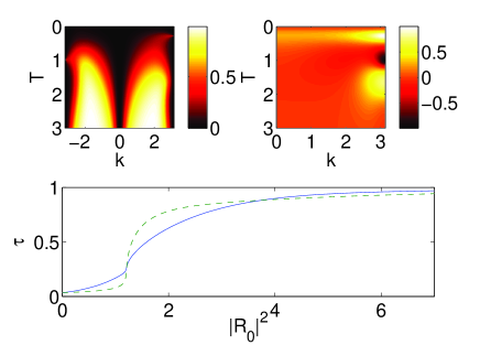
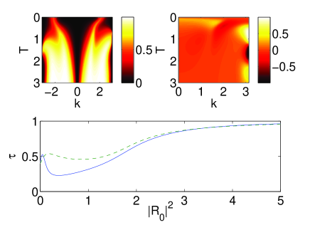
Figure 1: Each panel contains a contour plot of the transmission coefficient $\tau(k,T)$ (top left) and a contour plot of the rectification factor $f(k,T)$ of Equation (9) (top right), plotted as a function of $k$ and $T$. The panels also show a typical example of the dependence of $\tau$ for $k=2$ (solid lines) and $k=-2$ (dashed lines), so as to illustrate the asymmetry between the propagation for left and right incident waves (bottom panel). In the latter the dependence of $\tau$ is given as a function of $|R_{0}|^{2}$. The left panel corresponds to $N=2$ and $\gamma_{1}=2.5$, $\gamma_{2}=5$ and the lattice size is $L=200$ in this case. The right panel is the $N=3$ case with $\gamma_{1}=1.5$, $\gamma_{2}=2$ and $\gamma_{3}=3.5$; here the lattice size is $L=201$.

We seek standing wave solutions by setting $\phi_{n}=\psi_{n}e^{-i\omega t}$ for $\omega\in\mathds{R}$. This gives a set of algebraic equations which can be written in the form of a backwards transfer map

$$\psi_{n-1}=-\psi_{n+1}+\left(-\omega+\frac{\gamma_{n}\psi_{n}}{1+|\psi_{n}|^{2}}\right)\psi_{n}$$ (3)

for $\psi_{n}\in\mathds{C}$ independent of $t$. Following the procedure in D'A2012 and for now assuming $k\geq 0$, we begin by assuming solutions in the form of plane waves on the linear portions of the chain. That is,

$$\psi_{n}=\left\{\begin{array}[]{ll}R_{0}e^{ikn}+Re^{-ikn}&n\leq 1\\ Te^{ikn}&n\geq N\end{array}\right.$$ (4)

with $R_{0},R,T\in\mathds{C}$ representing the incident, reflected and transmitted amplitudes, respectively. The solution (4) solves Eq. (3) for $n\not\in\{1,\dots,N\}$ only if the wavenumber $k$ satisfies $\omega=-2\cos(k)$. Also directly from (4) with $n=0,1$ we have

$$R_{0}=\frac{e^{-ik}\psi_{0}-\psi_{1}}{e^{-ik}-e^{ik}}\qquad\mbox{ and }\qquad R=\frac{e^{ik}\psi_{0}-\psi_{1}}{e^{ik}-e^{-ik}}.$$ (5)

The stationary solution across the whole lattice is then known by the following procedure: given values for $\gamma_{n}$ for $n\in\{1,\dots,N\}$ we start by specifying values for $k$ and $T$. Then we compute $\psi_{0},\psi_{1},\dots\psi_{N-1}$ via Eq. (3) and then $R,R_{0}$ by (5). Such a procedure of finding the input as a function of the output is referred to as a “fixed output problem” knapp .

Stationary solutions where the amplitude $R_{0}$ is incident from the right-hand-side and the wavenumber is taken as $-k\leq 0$ can also be formulated in a similar way. In order to avoid swapping the format of (4) (so that $R_{0},R$ would apply on the right and $T$ on left), it is more convenient to leave (4) as-is with positive wave number $k$ and instead flip left-to-right the configuration of the nonlinearities, i.e. $\{\gamma_{1},\gamma_{2},\dots,\gamma_{N}\}\rightarrow\{\gamma_{N},\gamma_{N-1},\dots,\gamma_{1}\}$. In this way the computation of the solution for negative wavenumber is unchanged from the above outline aside from the swap of the order of the $\gamma$’s. Plots of these plane wave stationary solutions are shown in the next section, where we also address the stability of their $t$-propagation. In practice we truncate the lattice and refer to its finite length as $L$.

For a solution that has been determined by the processes described above, we next compute the transmission coefficient $\tau\stackrel{{\scriptstyle def.}}{{=}}|T|^{2}/|R_{0}|^{2}$ explicitly assuming that $T$ is given. For this purpose it is convenient to write $\psi_{n}\stackrel{{\scriptstyle def.}}{{=}}Te^{ikN}\Psi_{n}$ with $n=N-l$ so that $l=0$ corresponds to $n=N$, and incrementing $l$ corresponds to decreasing $n$. In this notation we have $\Psi_{N}=1$ for $l=0$ and the value of $\Psi_{n}$ for each subsequent node towards the left is given by rewriting Eq. (3) as

$$\Psi_{N-l}=-\Psi_{N-l+2}+\delta_{N-l+1}\Psi_{N-l+1}$$ (6)

for $\delta_{j}\stackrel{{\scriptstyle def.}}{{=}}-\omega+\frac{\gamma_{j}}{1+|T|^{2}|\Psi_{j}|^{2}}$. See the Appendix where we record a few iterations of Eq. (6). Then by (5) with $\psi_{0},\psi_{1}$ computed according to Eq. (6) we have

$$\begin{array}[]{lllllll}R_{0}=&{\frac{T}{e^{-ik}-e^{ik}}}\left(\delta_{1}-2e^{ik}\right)&&\tau=&\left|\frac{e^{ik}-e^{-ik}}{2e^{ik}-\delta_{1}}\right|^{2}&&\mbox{ \ for \ }N=1\\ R_{0}=&\frac{Te^{ik}}{e^{-ik}-e^{ik}}\left(-1+(\delta_{1}-e^{ik})(\delta_{2}-e^{ik})\right)&&\tau=&\left|\frac{e^{ik}-e^{-ik}}{1+(\delta_{1}-e^{ik})(e^{ik}-\delta_{2})}\right|^{2}&&\mbox{ \ for \ }N=2\end{array}$$ (7)

and

$$R_{0} = \frac{Te^{2ik}}{e^{-ik}-e^{ik}}\left(\delta_{1}-e^{ik}+(\delta_{3}-e^{ik})(1-\delta_{2}(\delta_{1}-e^{ik}))\right)$$

$$\tau = \left|\frac{e^{ik}-e^{-ik}}{e^{ik}-\delta_{1}+(e^{ik}-\delta_{3})(1-\delta_{2}(\delta_{1}-e^{ik}))}\right|^{2}\quad\mbox{ \ for \ }N=3.$$ (8)

In the linear case ($\gamma_{1}=\gamma_{2}=0$) and in the symmetric case ($\{\gamma_{1},\gamma_{2},\dots,\gamma_{N}\}=\{\gamma_{N},\gamma_{N-1},\dots,\gamma_{1}\}$ as an ordered set) it is immediately seen that $\tau$ is the same for waves incoming from the left or right side. For $N=1$ the transmission is always symmetric.

We also define here a quantity to measure the asymmetric propagation. We will use the definition of a rectification factor $f$ in the form of

$$f=\frac{\tau(k,T)-\tau_{flip}(k,T)}{\tau(k,T)+\tau_{flip}(k,T)}$$ (9)

where the quantity $\tau(k,T)$ corresponds to transmission of a left-incoming wave with positive wavenumber $k\geq 0$ and $\tau_{flip}(k,T)$ with $k\geq 0$ is equivalent to the transmission of a right-incoming wave with negative wavenumber (recall the process described above of keeping $k$ positive while flipping the order of the $\gamma$’s). This way nonzero values of $f$ in the range $[-1,1]$ measure the asymmetry of transmission in the system. Symmetry in transmission corresponds to $f=0$ and $f>0$ corresponds to greater transmission of incident waves originating from the left (transmitted on the right) as compared with incident waves originating from the right (transmitted on the left). Of course, $f<0$ corresponds to greater transmission of waves originating from the right.

Figure 1 shows plots of the transmission coefficient $\tau$ and the rectification factor $f$ as a function of the amplitude $T$ and the wavenumber $k$ of the extended plane wave solutions. We find that whether more is transmitted for waves incoming from the right or left is variable as a function of $k$ and $T$. Notice that values for $\gamma$’s are chosen in Figure 1 to be such that $\gamma_{1}<\gamma_{2}$ in the $N=2$ case and $\gamma_{1}<\gamma_{2}<\gamma_{3}$ in the $N=3$ case. In other words, with increasing $\gamma$’s from left to right we observe that transmission properties vary with the choice of the parameters $T,k$. We find that in accordance with our above analysis the $N=1$ case is symmetric. Although we do not show an $N=1$ analogue of Figure 1, such plots look similar to Fig. 1 but there is exact symmetry and $f=0$ for all $T,k$. It is interesting to point out here that the rectification factor appears to acquire its largest (absolute) values for $k$ close to $\pi$ i.e., at the edge of the Brillouin zone. Furthermore, both in the $N=2$ and in the $N=3$ case, the dependence of $f$ near this value appears to be a non-sign-definite function of $T$ (i.e., different ranges of $T$ values appear to favor propagation in one or the other direction).

III.2 Stability

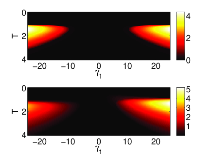
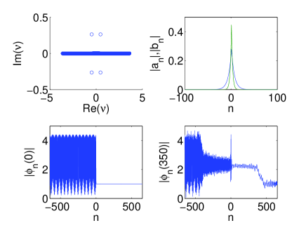
Figure 2: The left panel depicts the value of $|\min({\rm Im}(\nu)|$, for $N=1$, plotted as a function of $\gamma_{1}$ and $T$; the top graph shows $k=\pi/2$ and in the bottom graph $k=2.5$. The lattice length in the two left panel plots is $L=99$. These two plots show that the magnitude of the minimum imaginary part of the calculated eigenvalue, i.e. the strength of the instability, increases as the magnitude of $\gamma_{1}$ increases. On the other hand for a fixed $\gamma_{1}$ value an extended solution of the form shown in Eq. (4) is tending toward stabilization for large $T$. In the right panel we show four plots that correspond to a dim but nonzero region on the plot of $|\min({\rm Im}(\nu)|$ in the left panel. That is, the right-hand four plots correspond to $k=2.5$, $\gamma_{1}=5$ and $T=1$. The four plots show the eigenvalues in the complex plane (top left), eigenvector magnitude (top right with $|a_{n}|$ blue and $|b_{n}|$ green), initial profile of the plane wave at $t=0$ (bottom left) and a later profile at $t=350$ of the plane wave (bottom right). For this instability the eigenvalues are in the form of a quartet.

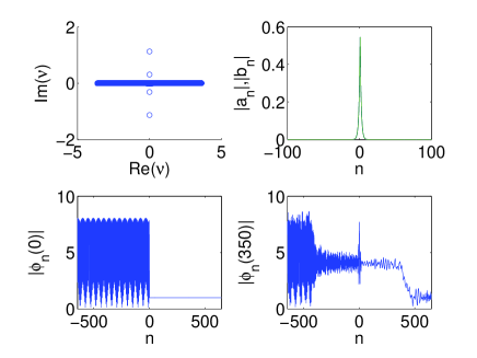
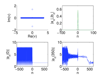
Figure 3: Here we focus on parameter values that correspond to a bright region in the left panel of Figure 2. We show four plots similar to the right panel of Figure 2. Here we have $N=1$, $L=1299$ and $k=2.5$. The left panel of four plots corresponds to $\gamma_{1}=9.5$, $T=1$, and the right panel corresponds to $\gamma_{1}=10$, $T=1.5$. Comparing the three sets of four plots in the present figure and in Figure 2 shows the transition in the eigenvalue plots as we move towards brighter regions of the $|\min({\rm Im}(\nu)|$ diagram.

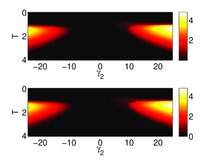
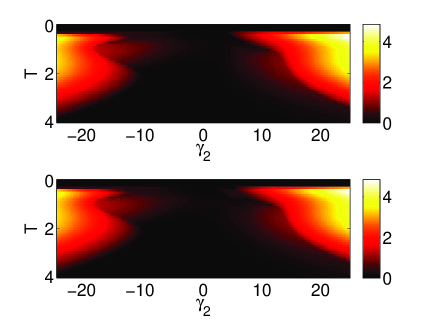
Figure 4: The plots are similar to the left panel in Fig. 2. Here the left panel corresponds to $N=2$, $L=100$ and we plot $|min(Im(\nu)|$ as a function of $\gamma_{2}$ and $T$ while the value of $\gamma_{1}$ is fixed: $\gamma_{1}=1$ in the top graph and $\gamma_{1}=-1$ in the bottom graph. Here the right panel corresponds to $N=3$, $L=101$ and we plot $|\min({\rm Im}(\nu)|$ as a function of $\gamma_{2}$ and $T$ while the values of $\gamma_{1}$ and $\gamma_{3}$ are fixed: $\gamma_{1}=1$, $\gamma_{3}=5$ in the top graph and $\gamma_{1}=-1$,$\gamma_{3}=5$ in the bottom graph.

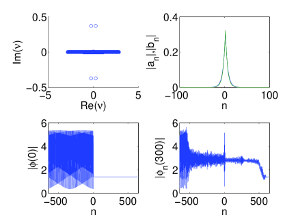
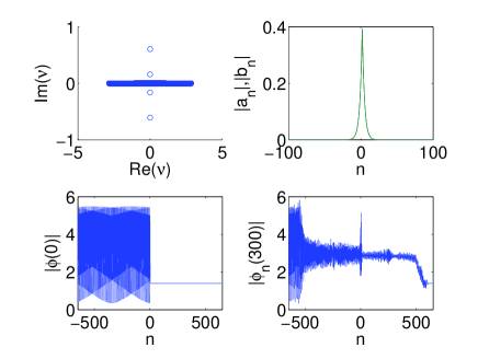
Figure 5: Here we focus on parameter values that correspond to the left panel of Figure 4. Again we show four plots similar to the right panel of Figure 2. Here we have $N=2$, $L=1300$ and $k=2$. The left panel of four plots corresponds to $\gamma_{1}=-1,\gamma_{2}=9.25$, $T=1.4$, and the right panel corresponds to $\gamma_{1}=-1,\gamma_{2}=9.5$, $T=1.4$. Comparing these two sets of four plots shows the transition in the eigenvalue plots as we move towards brighter regions of the appropriate $|min(Im(\nu)|$ diagram in Figure 4.

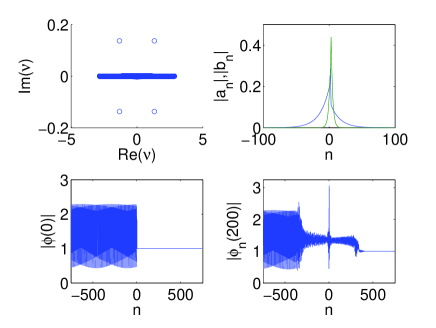
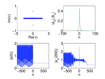
Figure 6: Here we focus on parameter values that correspond to the right panel of Figure 4. Again we show four plots similar to the right panel of Figure 2. Here we have $N=3$, $L=1301$ and $k=2$. The left panel of four plots corresponds to $\gamma_{1}=1,\gamma_{2}=3.25,\gamma_{3}=4$, $T=1$, and the right panel corresponds to $\gamma_{1}=1,\gamma_{2}=5.5,\gamma_{3}=4$, $T=0.4$. Comparing these two sets of four plots shows the transition in the eigenvalue plots as we move towards brighter regions of the appropriate $|min(Im(\nu))|$ diagram in Figure 4.

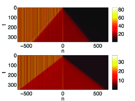
Figure 7: The plots show $|\phi_{n}(t)|^{2}$ as a function of $n$ and $t$. The top plot corresponds to parameters the same as in the right four plots in Fig. 3. The bottom plot corresponds to parameters the same as in the left four plots in Fig. 5.

In order to analyze spectral stability of stationary states of the form discussed in the previous subsection we write

$$\phi_{n}(t)=e^{-i\omega t}\left(\psi_{n}+\varepsilon\left(a_{n}e^{i\nu t}+b_{n}e^{-i\nu^{*}t}\right)\right)$$ (10)

for $a_{n},b_{n},\nu\in\mathds{C}$, $\varepsilon$ small, and with $\psi_{n}$ being a stationary solution from the previous section. The resultng linear stability equations then read

$$\nu\left(\begin{array}[]{c}a_{n}\\ b_{n}^{*}\end{array}\right)=\left(\begin{array}[]{cc}F_{1}&F_{2}\\ F_{3}&F_{4}\end{array}\right)\left(\begin{array}[]{c}a_{n}\\ b_{n}^{*}\end{array}\right)$$ (11)

for

$$F_{1}=diag\displaystyle\left(\omega-\frac{\gamma_{n}}{(1+|\psi_{n}|^{2})^{2}}\right)+G,\qquad F_{2}=diag\displaystyle\left(\frac{\gamma_{n}\psi_{n}^{2}}{(1+|\psi_{n}|^{2})^{2}}\right)$$ (12)

$$F_{3}=diag\displaystyle\left(\frac{-\gamma_{n}\psi_{n}^{2}}{(1+|\psi_{n}|^{2})^{2}}\right),\qquad F_{4}=diag\displaystyle\left(-\omega+\frac{\gamma_{n}}{(1+|\psi_{n}|^{2})^{2}}\right)-G$$

where $G$ is a sparse matrix with ones on both the super- and sub-diagonals. Given a stationary plane wave solution $\psi_{n}$ and values of $\gamma_{n}$ which encode the nonlinearity for $1\leq n\leq N$, one then calculates the eigenvalues $\nu$ in (11). If $\nu$ has a negative imaginary part this indicates that the perturbed solution $\phi_{n}(t)$ is unstable, as is easily seen by Eq. (10). In practice, one diagonalizes a finite truncation of the matrix in (11), ensuring that the relevant eigenvalues are not affected by the truncation error. In other words, $F_{1},F_{2},F_{3},F_{4}$ and $G$ are all $L\times L$ matrices and in the matrix Eq. (11) it is now convenient to think of $a_{n}$ and $b_{n}$ as length $L$ column vectors. Furthermore, the Hamiltonian symmetry of the solution ensures that the relevant instability eigenvalues come either in pairs (if $\nu$ is imaginary) or in quartets (if $\nu$ is genuinely complex).

In Figures 2, 4 we show a plot of $\min({\rm Im}(\nu))$ as a function of $T$ and $\gamma$. We find that an increase in the magnitude of a $\gamma_{i}$ parameter (with other nearby $\gamma$’s held fixed) leads to $\min({\rm Im}(\nu))$ of larger magnitude indicating greater instability. Figures 2, 3, 5, 6 show eigenvector and eigenvalue plots alongside snapshots of $\phi_{n}(t)$ to show the behaviour of typical propagation in the $t$ variable of the unstable plane waves. The boundary conditions are calculated according to (4) at $t=0$ and evolved by multiplying by $e^{-i\omega t}$ for $t>0$ so as to conform with (10). The unstable plane wave solution, when propagated in the evolution variable, exhibits a few effects: if $k>0$ then amplitude leaks over to the right-hand side (to the left if $k<0$), and due to the localized instability a peak appears in the center of the lattice. Of course, given the conservation laws of the system, the power $\sum_{n}|\phi_{n}(t)|^{2}$ and the Hamiltonian $\mathcal{H}(t)$ are preserved over $t$. The figures also show a transition in the eigenvalue plots for unstable solutions. A weak instability (corresponding to dim but nonzero regions of the $min(Im(\nu))$ plots of Figures 2, 4) results in eigenvalue plots in the complex plane where a quartet appears off the real axis; see Figures 2 and 5. As the instability is enhanced for larger values of $\gamma$ (comparably brighter regions of the $min(Im(\nu))$ plots), the two pairs constituting the quartet merges on the imaginary axis and subsequently split with one pair headed towards zero; see Figures 3, 5. For the highest magnitude of instability (brightest regions on the plots of $min(Im(\nu))$) the eigenvalues indicating the instability are in the form of a pair on the imaginary axis; see Figures 3, 6. In the examples shown, the instability generically appears to transport power to the right part of the lattice, deforming (decreasing the power of) the corresponding $n<0$ portion of the plane wave. On the other hand, critically (per the localized eigenvector of the instability), a localized mode appears to form at the central nonlinear nodes within the domain.

In comparing our results with that of casati , we find that the asymmetry associated with the saturable nonlinearity (presented here) is less pronounced to that of a system with a cubic nonlinearity and a linear potential term (presented in casati ). In the $t$ propagation of extended solutions we can also compare the top plot in Fig. 3 of casati with our Fig. 7 in which we show plots over space and the propagation parameter. The two systems both experience a concentration of amplitude at the center of the lattice as $t$ moves forward. In the case of the cubic nonlinearity in casati there are three concentrations of amplitude (two of which are moving). Here we see only the one central concentration of amplitude at the center while sites nearby the center drop amplitude in comparison to the highest points of the initialized state at $t=0$. Also, in contrast to casati where the amplitude concentrations more dramatically rise above the background, here the central concentration of amplitude is more similar to the maximal amplitude of the initialized state.

IV Propagation of a Gaussian

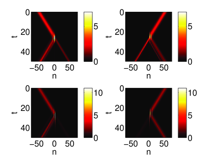
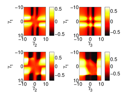
Figure 8: In the left four graphs, we plot $|\phi_{n}(t)|^{2}$ as a function of the lattice $n$ and the propagation variable $t$ for initial profile according to (13) with $|I|^{2}=2.5$. The left columns have wavenumber $k=\pi/2$ and starting position $n_{0}=-50$ and the right columns have wavenumber $k=-\pi/2$ and starting position $n_{0}=50$. The top two plots correspond to $N=2$ with $\gamma_{1}=2.75$ and $\gamma_{2}=5$; we calculate that the rectification factor in this case is $f\approx-0.1767$. The bottom two plots correspond to $N=3$ with $\gamma_{1}=3$, $\gamma_{2}=3.25$, $\gamma_{3}=4$; we calculate that $f\approx-0.1525$. In the right four graphs, we plot the rectification factor of the Gaussian waves for $N=2$ (left column) and $N=3$ (right column) as a function of variable $\gamma$ parameters. The top row corresponds to $|I|^{2}=1$ in (13) and the bottom row to $|I|^{2}=2.5$. For the $N=3$ plots, the value $\gamma_{2}=5$ (top) and $\gamma_{2}=3.25$ (bottom) is fixed.

Finally, in this section we look at the propagation of a Gaussian wavepacket through the lattice for each of the cases $N=1,2,3$. While it is less straightforward to prepare the delocalized initial conditions needed for the plane wave solutions of the previous section (whose asymmetric propagation, however, can be analytically quantified), preparing the Gaussian initial data of the present section appears to be considerably more tractable in optical experiments e.g., with lithium niobate waveguide arrays. On the other hand, in this latter setting, we will have to rely on detailed numerical computations of the rectification factor, as this set of initial conditions is less amenable to detailed analytical considerations. The wavepacket considered is given by the equation

$$\phi_{n}(0)=Ie^{-(n-n_{0})^{2}/s^{2}}$$ (13)

for starting position index $n_{0}$ and width parameter $s$. We measure the transmission at some value $t=t_{0}$ sufficiently large so that the wavepacket has interacted with the nonlinear region and, as a result, some portion of it has been accordingly transmitted through and reflected from the relevant interval. The transmission is then measured by

$$\tau_{+}=\frac{\sum_{n>N}|\phi_{n}(t_{0})|^{2}}{\sum_{n}|\phi_{n}(t_{0})|^{2}}\qquad\tau_{-}=\frac{\sum_{n<1}|\phi_{n}(t_{0})|^{2}}{\sum_{n}|\phi_{n}(t_{0})|^{2}}$$ (14)

for $k>0$ and $k<0$, respectively. Then the rectification factor takes the form $f=(\tau_{+}-\tau_{-})/(\tau_{+}+\tau_{-})$. The transmission is, of course, equal in both directions ($f=0$) in the $N=1$ case. In Figure 8 we plot $f$ as a function of $\gamma_{1},\gamma_{2}$ in the case of $N=2$, and as a function of $\gamma_{1},\gamma_{3}$ with $\gamma_{2}$ fixed in the case of $N=3$. In Figure 8 we also show some typical space-$t$ propagation plots for the Gaussian initial data case. Similar to the plane wave solutions case, the rectification factor may be positive or negative as the parameters change. Here the Gaussian in this particular case with $k=\pi/2$ has the following property. For parameter values concentrated in the vertical and horizontal bands in the right-side four plots of Fig. 8 more is transmitted if the wave hits the lower $\gamma$-value first, in comparison to the wave hitting the larger $\gamma$-value first, i.e., encountering the region which is closer to linear is more conducive towards transmission, while encountering the more nonlinear sites at first is more prone to reflection, a feature that seems to be intuitively justified.

V Conclusions

In the present work, we considered a lattice setting where embedded in a linear Schrödinger chain was a nonlinear “segment” of the saturable type. Our analytical considerations were focused around plane waves enabling us to analytically compute both the transmittivity and the rectification factor between left- and right-propagating such waves. These features evidence the asymmetric nature of the propagation in a way that is analytically tractable. This asymmetry can be explicitly traced in the nonlinearity of the relevant setup. We also considered the spectral stability of such states in which we observe some effects of low versus high rates of instability. Finally, we considered the asymmetry of propagation of a Gaussian wavepacket. The latter was also clearly evidenced both in the case of a dimer, as well as in that of a trimer, paving the way for the experimental observation of relevant phenomena, such as the enhanced transmission of a wavepacket when encountering a region of increasing, rather than that of a decreasing nonlinear index profile.

There are numerous aspects that may be worthwhile to further explore. In the context of lithium niobate waveguide arrays, it may be relevant to examine settings that involve a genuinely nonlinear lattice but with its central sites bearing a different nonlinearity than the background. This type of “spatial profile” of the nonlinearity coefficient has attracted considerable interest in numerous recent studies as evidenced by the review of kartashov and may also be quite experimentally tractable. On the other hand, the vast majority of the present studies on the nonlinearity-induced asymmetry that we are aware of have focused chiefly on one-dimensional configurations. However, it would be both more numerically challenging and also theoretically intriguing to explore scattering of two-dimensional wavepackets from a central (two-dimensional) segment of a lattice which is genuinely nonlinear. Such aspects are currently under investigation and will be reported in future publications.

Finally, we should note that after submission of this manuscript, we were notified of a related work in assun . While the models analyzed in these works are fairly similar, distinctive features of the present work are (a) that we explored systematically the stability of the extended waves and we studied the outcomes of their dynamical instabilities; and (b) we also considered the effect of the incidence of a Gaussian wave packet. Lastly, (c) although the latter work is restricted to dimers, our considerations here have been provided for general $N$ and examined for $N=1,2,3$.

VI Acknowledgements

The authors acknowledge useful discussions with Stefano Lepri on the subject. P.G.K acknowledges support from the National Science Foundation under grants CMMI-1000337, DMS-1312856, from ERC and FP7-People under the grant IRSES-606096 and from the US-AFOSR under grant FA9550-12-10332, as well as from the Binational Science Foundation under grant 2010239.

Appendix A Appendix

We show a few iterations of the backwards transfer map in (6).

$$\delta_{N} = -\omega+\frac{\gamma_{j}}{1+|T|^{2}}$$

$$\Psi_{N-1} = -e^{ik}+\delta_{N}$$

$$\delta_{N-1} = -\omega+\frac{\gamma_{N-1}}{1+|T|^{2}|\delta_{N}-e^{ik}|^{2}}$$

$$\Psi_{N-2} = -1+\delta_{N-1}(\delta_{N}-e^{ik})$$

$$\delta_{N-2} = -\omega+\frac{\gamma_{N-2}}{1+|T|^{2}|1+\delta_{N-1}(e^{ik}-\delta_{N})|^{2}}$$

$$\Psi_{N-3} = -\delta_{N-2}+(e^{ik}-\delta_{N})(1-\delta_{N-2}\delta_{N-1})$$

$$\delta_{N-3} = -\omega+\frac{\gamma_{N-3}}{1+|T|^{2}|\delta_{N-2}+(\delta_{N}-e^{ik})(1-\delta_{N-2}\delta_{N-1})|^{2}}$$

$$\Psi_{N-4} = 1-\delta_{N-3}\delta_{N-2}+(e^{ik}-\delta_{N})\left(\delta_{N-1}+\delta_{N-3}(1-\delta_{N-2}\delta_{N-1})\right)$$ (15)

References

- (1) Lederer, F.; Stegeman, G.I.; Christodoulides, D.N.; Assanto, G.; Segev, M.; Silberberg, Y. Discrete solitons in optics. Phys. Rep. 2008, 463, 1–126.
- (2) Morsch, O.; Oberthaler, M. Dynamics of Bose-Einstein condensates in optical lattices. Rev. Mod. Phys. 2006, 78, 179.
- (3) Sato, M.; Hubbard, B.E.; Sievers, A.J. Colloquium: Nonlinear energy localization and its manipulation in micromechanical oscillator arrays. Rev. Mod. Phys. 2006, 78, 137.
- (4) Binder, P.; Abraimov, D.; Ustinov, A.V.; Flach, S.; Zolotaryuk, Y. Observation of Breathers in Josephson Ladders. Phys. Rev. Lett. 2000, 84, 745.
- (5) Boechler, N.; Theocharis, G.; Job, S.; Kevrekidis, P.G.; Porter, M.A.; Daraio, C. Discrete Breathers in One-Dimensional Diatomic Granular Crystals. Phys. Rev. Lett. 2010, 104, 244302.
- (6) English, L.Q.; Sato, M.; Sievers, A.J. Modulational instability of nonlinear spin waves in easy-axis antiferromagnetic chains. II. Influence of sample shape on intrinsic localized modes and dynamic spin defects. Phys. Rev. B 2003, 67, 024403.
- (7) Swanson, B.I.; Brozik, J.A.; Love, S.P.; Strouse, G.F.; Shreve, A.P.; Bishop, A.R.; Wang, W.-Z.; Salkola, M.I. Observation of Intrinsically Localized Modes in a Discrete Low-Dimensional Material. Phys. Rev. Lett. 1999, 82, 3288.
- (8) Peyrard, M. Nonlinearity. 2004, 17, R1.
- (9) Kosevich, Y. A. Fluctuation subharmonic and multiharmonic phonon transmission and Kapitza conductance between crystals with very different vibrational spectra. Phys. Rev. B 1995, 52, 1017.
- (10) Terraneo, M.; Peyrard, M.; Casati, G. Controlling the Energy Flow in Nonlinear Lattices: A Model for a Thermal Rectifier. Phys. Rev. Lett. 2002, 88, 094302.
-
(11)
Chang, C.W.; Okawa, D.; Majumdar, A.; Zettl, A. Solid-state thermal rectifier.
Science. 2006, 314, 1121.
Kobayashi, W.; Teraoka, Y.; Terasaki, I. An oxide thermal rectifier. Appl. Phys. Lett. 2009, 95, 171905. -
(12)
Scalora, M.; Dowling, J.P.; Bowden, C.M.;
Bloemer, M.J. The photonic band edge optical diode. J. Appl. Phys. 1994, 76, 2023
Tocci, M.D.; Bloemer, M.J.; Scalora, M.; Dowling, J.P.; Bowden, C.M. Thinfilm nonlinear optical diode. Appl. Phys. Lett. 1995, 66, 2324. - (13) Konotop, V.V.; Kuzmiak, V. Nonreciprocal frequency doubler of electromagnetic waves based on a photonic crystal. Phys. Rev. B 2002, 66, 235208.
- (14) Gallo, K.; Assanto, G.; Parameswaran, K.; Fejer, M. All-optical diode in a periodically poled lithium niobate waveguide. Appl. Phys. Lett. 2001, 79, 314.
- (15) Feise, M.W.; Shadrivov, I.V.; Kivshar, Y.S. Bistable diode action in left-handed periodic structures. Phys. Rev. E 2005, 71, 037602.
-
(16)
Boechler, N.; Theocharis, G.; Daraio, C. Bifurcation-based acoustic switching and rectification.
Nature Mater. 2011, 10, 665
Liang, B.; Yuan, B.; Cheng, J.C. Acoustic Diode: Rectification of Acoustic Energy Flux in One-Dimensional Systems. Phys. Rev. Lett. 2009, 103, 104301
Liang, B.; Guo, X.S.; Tu, J.; Zhang, D.; Cheng, J.C. An acoustic rectifier. Nature Mater. 2010, 9, 989-992. -
(17)
Lin, Z.; Ramezani, H.; Eichelkraut, T.; Kottos, T.; Cao, H.; Christodoulides, D.N. Unidirectional Invisibility Induced by -Symmetric Periodic Structures. Phys. Rev. Lett. 2011, 106, 213901.
Bender, N.; Factor, S.; Bodyfelt, J.D.; Ramezani, H.; Christodoulides, D.N.; Ellis, F.M.; Kottos, T. Observation of Asymmetric Transport in Structures with Active Nonlinearities. Phys. Rev. Lett. 2013, 110, 234101. - (18) D’Ambroise, J.; Kevrekidis, P.G.; Lepri, S. Asymmetric wave propagation through nonlinear -symmetric oligomers. J. Phys. A: Math. Theor. 2012, 45, 444012.
- (19) Lepri, S.; Casati, G. Asymmetric wave propagation in nonlinear systems. Phys. Rev. Lett. 2011, 106, 164101
- (20) Kevrekidis, P.G. The Discrete Nonlinear Schrödinger Equation; Springer-Verlag: Heidelberg, Germany, 2009.
- (21) Smirnov, E.; Rüter, C.E.; Stepić, M.; Kip, D.; Shandarov, V. Formation and light guiding properties of dark solitons in one-dimensional waveguide arrays. Phys. Rev. E 2006, 74, 065601.
- (22) Dong, R.; Rüter, C.E.; Song, D.; Xu, J.; Kip, D. Formation of higher-band dark gap solitons in one dimensional waveguide arrays. Opt. Express 2010, 18, 27493.
- (23) Dong, R.; Rüter, C.E.; Kip, D.; Cuevas, J.; Kevrekidis, P.G.; Song, D.; Xu, J. Dark-bright gap solitons in coupled-mode one-dimensional saturable waveguide arrays. Phys. Rev. A 2011, 83, 063816.
- (24) Kanshu, A.; Rüter, C.E.; Kip, D.; Cuevas, J.; Kevrekidis, P.G. Dark lattice solitons in one-dimensional waveguide arrays with defocusing saturable nonlinearities and alternating couplings. Eur. Phys. J. D 2012, 66, 182.
- (25) Samuelsen, M.R.; Khare, A.; Saxena, A.; Rasmussen, K.O. Statistical mechanics of a discrete Schrödinger equation with saturable nonlinearity. Phys. Rev. E 2013, 87, 044901.
- (26) Knapp, R.; Papanicolaou, G.; White, B. Transmission of waves by a nonlinear random medium. J. Stat. Phys. 1991, 63, 567.
- (27) Kartashov, Y.V.; Malomed, B.A.; Torner, L. Solitons in nonlinear lattices. Rev. Mod. Phys. 2011, 83, 247.
- (28) Assunçao, T.F.; Nascimento, E.M.; Lyra, M.L. Nonreciprocal transmission through a saturable nonlinear asymmetric dimer. Phys. Rev. E 2014, 90, 022901.