Spectroscopy of SU(4) lattice gauge theory with fermions in the two index anti-symmetric representation

Abstract:

We present a study of spectroscopy of $SU(4)$ lattice gauge theory coupled to two flavors of Dirac fermions in the anti-symmetric two index representation. The fermion representation is real, and the pattern of chiral symmetry breaking is $SU(2N_{f})\rightarrow SO(2N_{f})$ with $N_{f}$ flavors of Dirac fermions. It is an interesting generalization of QCD, for several reasons: it allows direct exploration of an alternate large $N_{c}$ expansion, it can be simulated at non-zero chemical potential with no sign problem, and several UV completions of composite Higgs systems are built on it. We present preliminary results on the baryon and meson spectra of the theory and compare them with $SU(3)$ results and with expectations for large $N_{c}$ scaling.

1 Introduction

The authors of this paper are involved in a diverse set of projects involving $SU(4)$ gauge theory with various numbers of flavors of degenerate mass fermions in the two-index antisymmetric (AS2) representation of the gauge group, which is a sextet for $SU(4)$. These systems are interesting for a variety of reasons:

First, they are confining and chirally broken systems with similarities to ordinary $N_{c}=3$ QCD. In fact, there is an alternate large-$N_{c}$ limit of ordinary QCD in which the fermions live in an AS2 representation. For $N_{c}=3$, AS2 quarks inhabit the $\bar{3}$ representation. The story goes back to [1]. It reappears in more modern guises in, for example, [2, 3]. Lattice simulation can test the expected large-$N_{c}$ regularities, as it has for the usual ’t Hooft limit of fixed $N_{f}$ fundamental representation fermions at varying $N_{c}$. (An assortment of recent results includes [4, 5].)

Next, they form a chirally broken system with some differences compared to ordinary $N_{c}=3$ QCD. Because the fermions are in a real representation of the gauge group, the pattern of chiral symmetry breaking is not $SU(N_{f})\otimes SU(N_{f})\rightarrow SU(N_{f})$; it is $SU(2N_{f})\rightarrow SO(2N_{f})$ (all for $N_{f}$ flavors of Dirac fermions) [6]. The reality of the representation allows quarks and antiquarks to mix under global flavor rotations. In particular, the $N_{f}=2$ theory has nine Goldstone bosons, which may be classified as isospin $I=1$ triplets of $q\bar{q}$, $qq$, and $\bar{q}\bar{q}$.

Third, reality of the representation means that finite density simulations do not suffer from a sign problem. This is similar to the situation for $N_{c}=2$ with fundamental representation fermions [7]. There is a literature of predictions for $SU(4)$ [8], which we can explore.

Finally, members of this family play a role in composite Higgs studies. For example, the Littlest Higgs model [9] relies on the non-linear sigma model $SU(5)/SO(5)$. Examples of proposed $SU(4)$ UV completions of composite Higgs models, mostly involving 5 Majorana fermions, are given in Refs. [10].

In this note we describe results relevant to the first of these points. The details of the calculations will be presented in our longer paper [11].

2 Lattice setup and observables

We use the usual Wilson plaquette gauge action and Wilson-clover fermions with nHYP smeared links as the gauge connections. The bare gauge coupling $g$ is defined through $\beta=2N_{c}/g^{2}$. The bare quark mass $m$ is introduced through the hopping parameter $\kappa$. The clover coefficient is fixed at its tree level value, $c_{sw}=1$.

Simulations were done at four different $\kappa$ values at a bare coupling $\beta=9.6$. The lattice volume is fixed to be $16^{3}\times 32$. In addition, we calculated spectroscopy at four more partially quenched (PQ) points based on one dynamical data set.

Our large-$N_{c}$ comparisons are done against simulations of $SU(3)$ gauge theory with $N_{f}=2$ fundamental fermions. Five different $\kappa$ values were used at one fixed gauge coupling. Previously generated quenched $SU(N_{c})$ theories, with $N_{c}=3$, 5, and 7 are also used for comparison [12]. All these data sets had the same volume, $16^{3}\times 32$. For comparison among different theories, we fix the lattice spacings using $r_{1}$, the shorter version [13] of the Sommer [14] parameter, defined in terms of the force $F(r)$ between static quarks: $r^{2}F(r)=-1.0$ at $r=r_{1}$.

The pseudoscalar and vector meson decay constants $f_{PS}$ and $f_{V}$ are defined below in Eqs. (1) and (2); and the quark mass $m_{q}$ is defined from the axial Ward identity (AWI) Eq. (3).

$$\langle 0|\bar{u}\gamma_{0}\gamma_{5}d|PS\rangle=m_{PS}f_{PS},$$ (1)

$$\langle 0|\bar{u}\gamma_{i}d|V\rangle=m_{V}^{2}f_{V}\epsilon_{i},$$ (2)

$$\partial_{t}\sum_{\bf x}\left\langle A_{0}^{a}({\bf x},t){\cal O}^{a}\right\rangle=2m_{q}\sum_{\bf x}\left\langle P^{a}({\bf x},t){\cal O}^{a}\right\rangle.$$ (3)

$A_{\mu}^{a}=\bar{\psi}\gamma_{\mu}\gamma_{5}(\tau^{a}/2)\psi$ is the axial current, $\vec{\epsilon}$ is a polarization vector, $P^{a}=\bar{\psi}\gamma_{5}(\tau^{a}/2)\psi$ is the pseudoscalar density, and ${\cal O}^{a}$ is a source. In our normalization convention $f_{PS}\approx 132$ MeV. In Eqs. (1) and (2), the lattice decay constants need to be renormalized by a field rescaling and the corresponding $Z$ factors to get the continuum quantities. For the pseudoscalar decay constant, we have

$$f_{PS}^{cont}=\left(1-\frac{3}{4}\frac{\kappa}{\kappa_{c}}\right)Z_{PS}f_{PS}^{latt}.$$ (4)

There is a similar equation for the vector case. For our case, the $Z$ factors are close to unity [11, 15].

3 Phase diagram

Before computing spectroscopy, we have to map out the phase structure of the system in the $(\beta,\kappa)$ plane. The result is shown in Fig. 1. It is a bit complicated. Here are the ingredients:

Running along the top right side of the figure is the $\kappa_{c}$ line, where the AWI quark mass vanishes. The steeply falling line on the left is a bulk transition. It appears to be first order out to $\beta=9.7$, and then seems to turn into a crossover. When it is first order, the quark mass jumps discontinuously. We believe that the $\kappa_{c}$ line disappears when it encounters this transition, so that at sufficiently strong coupling there is no zero quark mass point for this lattice action.

The region between the two lines contains the desired confining and chirally broken phase. We did simulations on asymmetric lattices and observed finite temperature transitions from a confined to a deconfined phase. These lines move to bigger $\beta$ as the temporal size of the lattice increases. We wanted to simulate at lattice spacings which were neither too large or too small. We settled on a line varying $\kappa$ at $\beta=9.6$.

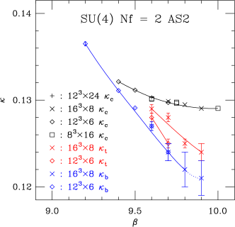
Figure 1: Phase diagram of the $SU(4)$ AS2 theory in the ($\beta$, $\kappa$) plane. The solid lines are drawn to guide the eye and are not a fit to the data. From right to left: the $\kappa_{c}$ line, the thermal transition lines $\kappa_{t}(N_{t}=8)$ and $\kappa_{t}(N_{t}=6)$, and the bulk transition line $\kappa_{b}$. The dotted line indicates weakening of the bulk transition to a crossover.

4 Large $N_{c}$ scaling tests

We computed the masses of the pseudoscalar and vector mesons and their decay constants, and the masses of $J=0$ and $J=1$ diquark states, which were degenerate with their mesonic analogs, as expected (this should no longer be true if a chemical potential is turned on). Meson masses are expected to be $N_{c}$ independent, regardless of the fermion representation.

Pseudoscalar and vector meson decay constants $f$ scale differently with $N_{c}$ in the fundamental and AS2 representations. The expected large $N_{c}$ scaling behavior is

$$f\sim\left\{\begin{array}[]{r l}\sqrt{N_{c}}&\quad\textrm{fundamental,}\\ N_{c}&\quad\textrm{AS2.}\end{array}\right.\$$ (5)

In leading order in $N_{c}$, baryon masses scale with the number of quarks ($N_{b}$) in the baryon, with corrections. $N_{b}=N_{c}$ for fundamental representation fermions, of course, and $N_{b}=N_{c}(N_{c}-1)/2$ for AS2 fermions [16]. This means that $N_{b}=6$ for our $N_{c}=4$ case. This is easy to understand by noting that the AS2 representation of $SU(4)$ is equivalent to the vector representation of $SO(6)$, and the color singlet baryon wave function is just the antisymmetric product of six vectors. At order $1/N_{b}$, the baryon mass $M_{B}$ is given by the rotor formula [17, 18]

$$M_{B}(J)~{}\approx~{}N_{b}m_{0}+B\frac{J(J+1)}{N_{b}}.$$ (6)

The parameters $m_{0}$ and $B$ depend on the quark mass. These are just the leading terms in a $1/N_{c}$ expansion. For example, $m_{0}=m_{00}+(1/N_{c})m_{01}+(1/N_{c}^{2})m_{02}+\cdots$. The terms in the expansion, such as $m_{01}$, are expected to have some “typical hadronic size.” This generic behavior is also expected for meson masses and decay constants.

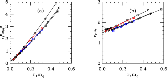
Figure 2: Meson spectroscopy. On the left, the squared pseudoscalar mass scaled by $r_{1}^{2}$, on the right, $r_{1}$ times the vector meson mass. The abscissa is $r_{1}$ times the AWI quark mass. The data sets are: black squares for quenched $SU(3)$ fundamentals, black diamonds for quenched $SU(5)$ fundamentals, black octagons for quenched $SU(7)$ fundamentals, red crosses for $SU(4)$ AS2; the fancy diamonds are the PQ data. Finally, the blue squares are $SU(3)$ with two dynamical, fundamental flavors.

In Fig. 2, we plot the data for the pseudoscalar and vector meson masses as a function of the AWI quark mass $m_{q}$. The weak dependence of meson masses on $N_{c}$ and representation confirms large-$N_{c}$ expectations.

To compare decay constants at different $N_{c}$, we follow Eq. (5) and rescale the fundamental representation data by $\sqrt{3/N_{c}}$, and the AS2 data by $3/N_{c}$. In Fig. 3, we plot the rescaled pseudoscalar and vector meson decay constants in $r_{1}$ units. Dynamical $SU(3)$ data overlap well with all the different $N_{c}$ quenched fundamental ones. The $SU(4)$ AS2 data is consistently above the fundamental ones, but the discrepancy is less than $20\%$.

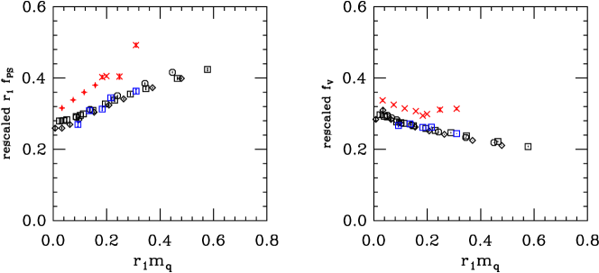
Figure 3: Pseudoscalar and vector meson decay constants. The abscissa is $r_{1}$ times the AWI quark mass. The meaning of the symbols is the same as in Fig. 2. The data are rescaled according to Eq. (5) as described in the text.

Baryon mass data are shown in Fig. 4.

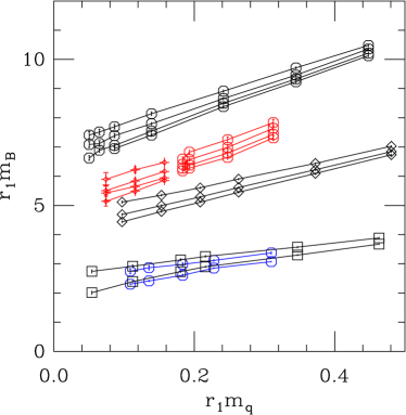
Figure 4: Baryons. The black data are (from the top) quenched $SU(7)$, $SU(5)$ and $SU(3)$ data. The blue octagons are $SU(3)$ with dynamical fermions. The red lines are the six quark baryons in $SU(4)$ AS2, octagons for dynamical and fancy diamonds for partially quenched. Higher $J$ states lie higher in mass and equal $J$ value points are connected by lines.

To compare to the rotor formula, we fit the data with Eq. (6) treating $m_{0}$ and $B$ as free parameters. The fit results are shown in the left panel of Fig. 5 for AS2 data at one quark mass, corresponding to $\kappa=0.1285$. The squares are the fit results and the octagons with error bars are the data points. The correlation between the parameters $m_{0}$ and $B$ at different quark masses is shown in the right panel of Fig. 5. The slope of $r_{1}B$ versus $1/({r_{1}}{m_{0}})$ is around one in the log-log plot. This suggests that the parameter $B$ is inversely proportional to $m_{0}$: this is consistent with the rotor formula, since $N_{B}/(2B)$ is the baryon’s moment of inertia.

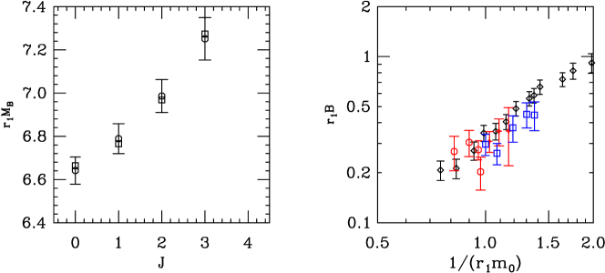
Figure 5: Left: Fit to rotor formula. $SU(4)$ AS2; $\kappa=0.1285$. Octagons with error bars are the data points; squares the best fit values. Right: $B$ vs. $m_{0}$ from the rotor formula; black diamonds from quenched $SU(3)$, blue squares from full $SU(3)$. The $SU(4)$ data are shown as red octagons for the dynamical sets and fancy diamonds for the partially quenched set.

5 Conclusions

Large-$N_{c}$ scaling certainly seems to describe all of our data, both with fundamental and AS2 fermions. Even the quantities with the poorest agreement, the decay constants, show only a twenty per cent discrepancy. Phenomenologists commonly use large-$N_{c}$ scaling to move from QCD to other confining theories. Lattice simulations show that this is a reasonable thing to do.

Our large-$N_{c}$ story for AS2 fermions is still incomplete. With only two $N_{c}$’s, one cannot do any kind of detailed analysis. Additionally, $SU(4)$ with AS2 fermions is also special in its pattern of chiral symmetry breaking compared to all other $N_{c}$’s. We plan to continue our studies of this curious system.

- [1] E. Corrigan and P. Ramond, Phys. Lett. B 87, 73 (1979).
- [2] A. Armoni, M. Shifman and G. Veneziano, Phys. Rev. Lett. 91, 191601 (2003) [hep-th/0307097]. A. Armoni, M. Shifman and G. Veneziano, Nucl. Phys. B 667, 170 (2003) [hep-th/0302163].
- [3] A. Cherman, T. D. Cohen and R. F. Lebed, Phys. Rev. D 86, 016002 (2012) [arXiv:1205.1009 [hep-ph]].
- [4] B. Lucini and M. Panero, Phys. Rept. 526, 93 (2013) [arXiv:1210.4997 [hep-th]].
- [5] G. S. Bali, F. Bursa, L. Castagnini, S. Collins, L. Del Debbio, B. Lucini and M. Panero, JHEP 1306, 071 (2013) [arXiv:1304.4437 [hep-lat]].
- [6] M. E. Peskin, Nucl. Phys. B 175, 197 (1980).
- [7] J. B. Kogut, M. A. Stephanov, D. Toublan, J. J. M. Verbaarschot and A. Zhitnitsky, Nucl. Phys. B 582, 477 (2000) [hep-ph/0001171]; J. B. Kogut, D. Toublan and D. K. Sinclair, Nucl. Phys. B 642, 181 (2002) [hep-lat/0205019]; S. Hands, S. Kim and J. -I. Skullerud, Eur. Phys. J. C 48, 193 (2006) [hep-lat/0604004]; S. Cotter, P. Giudice, S. Hands and J. -I. Skullerud, Phys. Rev. D 87, 034507 (2013) [arXiv:1210.4496 [hep-lat]].
- [8] M. Blake and A. Cherman, Phys. Rev. D 86, 065006 (2012) [arXiv:1204.5691 [hep-th]]; A. Cherman, M. Hanada and D. Robles-Llana, Phys. Rev. Lett. 106, 091603 (2011) [arXiv:1009.1623 [hep-th]]; M. I. Buchoff, A. Cherman and T. D. Cohen, Phys. Rev. D 81, 125021 (2010) [arXiv:0910.0470 [hep-ph]].
- [9] N. Arkani-Hamed, A. G. Cohen, E. Katz and A. E. Nelson, JHEP 0207, 034 (2002) [hep-ph/0206021].
- [10] L. Vecchi, arXiv:1304.4579 [hep-ph]. G. Ferretti and D. Karateev, JHEP 1403, 077 (2014) [arXiv:1312.5330 [hep-ph]]. G. Ferretti, JHEP 1406, 142 (2014) [arXiv:1404.7137 [hep-ph]].
- [11] T. DeGrand, Y. Liu, E. Neil, Y. Shamir and B. Svetitsky, in preparation.
- [12] T. DeGrand, Phys. Rev. D 86, 034508 (2012) [arXiv:1205.0235 [hep-lat]].
- [13] C. W. Bernard, T. Burch, K. Orginos, D. Toussaint, T. A. DeGrand, C. E. DeTar, S. A. Gottlieb and U. M. Heller et al., Phys. Rev. D 62, 034503 (2000) [hep-lat/0002028].
- [14] R. Sommer, Nucl. Phys. B 411, 839 (1994) [arXiv:hep-lat/9310022].
- [15] T. A. DeGrand, A. Hasenfratz and T. G. Kovacs, Phys. Rev. D 67, 054501 (2003) [hep-lat/0211006].
- [16] S. Bolognesi, Phys. Rev. D 75, 065030 (2007) [hep-th/0605065].
- [17] G. S. Adkins, C. R. Nappi and E. Witten, Nucl. Phys. B 228, 552 (1983).
- [18] E. E. Jenkins, Phys. Lett. B315, 441-446 (1993). [hep-ph/9307244].