The Occurrence of Earth-Like Planets Around Other Stars

Abstract

The quantity $\eta_{\oplus}$, the number density of planets per star per logarithmic planetary radius per logarithmic orbital period at one Earth radius and one year period, describes the occurrence of Earth-like extrasolar planets. Here we present a measurement of $\eta_{\oplus}$ from a parameterised forward model of the (correlated) period-radius distribution and the observational selection function in the most recent (Q17) data release from the Kepler satellite. We find $\eta_{\oplus}=3.9_{-1.6}^{+2.2}\%$ (90% CL). We conclude that each star hosts $3.83_{-0.62}^{+0.76}$ planets with $P\lesssim 3\mathrm{yr}$ and $R\gtrsim 0.2R_{\oplus}$. Our empirical model for false-positive contamination is consistent with the dominant source being background eclipsing binary stars. The distribution of planets we infer is consistent with a highly-stochastic planet formation process producing many correlated, fractional changes in planet sizes and orbits.

1. Introduction

The quantity $\eta_{\oplus}$, the number density of planets per star per logarithmic planetary radius per logarithmic orbital period at one Earth radius and one year period, describes the occurrence of Earth-like extrasolar planets. Measurement of $\eta_{\oplus}$ is complicated by the difficulty of detecting Earth-like planets in Earth-like orbits about Sun-like stars. Here we present a measurement of $\eta_{\oplus}$ from a parameterised forward model of the (correlated) period-radius distribution and the observational selection function in the most recent (Q17) data release from the Kepler satellite (Borucki et al., 2010, 2011; Batalha et al., 2013). Our data set comprises 181,568 systems observed under the Kepler exoplanet observing program (mostly G-type stars on the main sequence (Batalha et al., 2010)), producing 2598 planetary candidates. We parameterise the distribution of planetary periods and radii using a single, correlated Gaussian component; treat selection effects using a parameterised transit detection probability based on the measured noise level and stellar properties in the Kepler catalog; and include an empirically-parameterised, independent component in the period-radius distribution to represent false-positive planet detections. Using our model we can simultaneously estimate $\eta_{\oplus}$, place constraints on the planet period-radius distribution function, and determine the degree of contamination by false-positive candidate identifications. We find $\eta_{\oplus}=3.9_{-1.6}^{+2.2}\%$ (90% CL). We conclude that each star hosts $3.83_{-0.62}^{+0.76}$ planets with $P\lesssim 3\mathrm{yr}$ and $R\gtrsim 0.2R_{\oplus}$, that the peak of the planet radius distribution lies at $R_{\mathrm{peak}}=1.25_{-0.17}^{+0.16}R_{\oplus}$, and that $\ln P$ and $\ln R$ are correlated with correlation coefficient $r=0.334_{-0.053}^{+0.052}$ (all 90% CL). Our empirical model for false-positive contamination is consistent with the dominant source being background eclipsing binary stars (Fressin et al., 2013), with $7.8_{-1.3}^{+1.4}\%$ (90% CL) of the candidates being false-positives. The distribution of planets we infer is consistent with a highly-stochastic planet formation process producing many correlated, fractional changes in planet sizes and orbits. Our approach of determining both the intrinsic distribution of objects and selection effects empirically from survey data is generally applicable.

The Kepler satellite detects planets by observing a decrement in the photometric intensity of a planet’s host star as the planet transits between the telescope and the star. The Q17 data release describes 2598 “candidate” planetary transit signals identified by the Kepler team from observations of stars in the “EX” observing program (which are primarily G-type main-sequence stars similar to our own Sun (Batalha et al., 2010)), giving the inferred planetary period and radius for each. The fractional depth of a planetary transit signal depends only on the radii of the planet and its host star. The signal to noise ratio of a series of transits about a particular star in the Kepler satellite scales with planetary period and radius as (Chatterjee et al., 2012)

$$\rho=\rho_{0}\left(\frac{R}{R_{\oplus}}\right)^{2}\left(\frac{P}{1\,\mathrm{yr}}\right)^{-1/3},$$ (1)

where $\rho_{0}$ is the signal to noise ratio of a Earth-radius planet in a one-year orbit about that star, which depends on the number of quarters of observation of that star, the stellar radius and mass, and the intrinsic variability of the stellar intensity (Christiansen et al., 2012). In our analysis, we obtain these quantities from the Kepler Input Catalog (Batalha et al., 2010; Brown et al., 2011) and the MAST Kepler archive.

2. Model

To a good approximation (see Fig. 4 below), the detectability of a series of planetary transits in the Kepler data set is a function of the signal to noise ratio of the series. Because the detectability of planet transits depends on both period and radius, it is important to consider the joint (i.e., two-dimensional) distribution of these quantities in the data (Tabachnik & Tremaine, 2002; Youdin, 2011). We model the detection probability of a transit as a function that rises linearly in the log of the signal to noise ratio from zero at a threshold signal to noise to one at a larger signal to noise:

$$p_{\mathrm{detect}}=\begin{cases}0&\rho<\rho_{\mathrm{min}}\\ \frac{\log\rho-\log\rho_{\mathrm{min}}}{\log\rho_{\mathrm{max}}-\log\rho_{\mathrm{min}}}&\rho_{\mathrm{min}}<\rho<\rho_{\mathrm{max}}\\ 1&\rho_{\mathrm{max}}<\rho\end{cases},$$ (2)

where $\rho_{\mathrm{min}}$ and $\rho_{\mathrm{max}}$ are parameters of our model. We find $\rho_{\mathrm{min}}=5.46^{+0.18}_{-0.18}$ and $\rho_{\mathrm{max}}=18.8^{+1.9}_{-1.9}$ (90% CL), in rough agreement with Borucki et al. (2011); Batalha et al. (2013). A plot of our inferred detection probability appears in Fig. 1

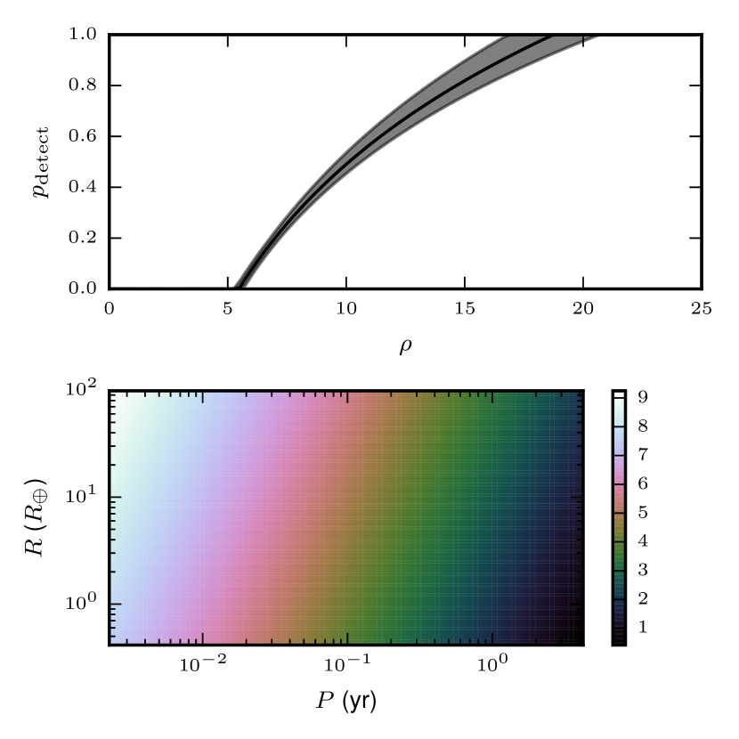
Figure 1.— Inferred detection probability and density of background contamination. (Top) The inferred detection probability versus signal-to-noise ratio (see Eq. (2)) from our parameterised model of selection effects. The solid line is the posterior median detection probability and the shading gives the 90% credible posterior interval. Our inferred detection probability is in rough agreement with the measurements of detection efficiency in Borucki et al. (2011); Batalha et al. (2013). (Bottom) The number density of false-positive candidate signals, $dN_{\mathrm{bg}}/d\ln P\,d\ln R$ (see Eq. (6)). The density is highest at small candidate period and large radius, consistent with the dominant source of contamination being background eclipsing binaries (Fressin et al., 2013). Overall, our model finds $7.8_{-1.3}^{+1.4}\%$ of the candidates are false-positive background signals, consistent with the analysis in Fressin et al. (2013).

The probability that a planet’s orbital plane will align with the line-of-sight to Earth and thereby produce a transit signal is

$$p_{\mathrm{transit}}=0.0016\,\frac{R_{\mathrm{star}}}{R_{\odot}}\left(\frac{M_{\mathrm{star}}}{M_{\odot}}\right)^{-1/3}\left(\frac{P}{1\,\mathrm{yr}}\right)^{-2/3}.$$ (3)

Putting Eq. 2 and 3 together, the probability that Kepler will detect a planet of radius $R$ orbiting its host star at period $P$ is

$$p_{\mathrm{select}}=p_{\mathrm{transit}}p_{\mathrm{detect}}.$$ (4)

A correlated log-normal distribution of planets in period and radius would be a natural outcome of a stochastic planet formation process that produced many correlated, fractional changes in planet sizes and orbits. As we shall see (Figure 4), this simple model combined with the aforementioned selection function provides a good fit to the Kepler candidate distribution. In our model, observed planets populate the candidate $P$-$R$ plane with number density

$$\frac{dN_{\mathrm{obs}}}{d\ln P\,d\ln R}=\left[\sum_{\mathrm{stars}}p_{\mathrm{select}}(P,R)\right]\\ \times\Lambda_{\mathrm{pl}}N\left[\mu,\Sigma\right]\left(\ln P,\ln R\right),$$ (5)

where $\Lambda_{\mathrm{pl}}$, $\mu$, and $\Sigma$ are parameters of our model, with $\Lambda_{\mathrm{pl}}$ the average number of planets per star, $\mu=\left[\mu_{P},\mu_{R}\right]$ the mean of $\ln P$ and $\ln R$, and $\Sigma=\left[\left[\Sigma_{PP},\Sigma_{PR}\right],\left[\Sigma_{PR},\Sigma_{RR}\right]\right]$ the covariance matrix of $\ln P$ and $\ln R$; $N\left[\mu,\Sigma\right](x,y)$ is the normal distribution. Our model assumes that planets appear around their host stars in a Poisson process; this is almost certainly wrong in detail (Weissbein et al., 2012), but nevertheless provides a good fit to the observed data (see Figure 4).

In addition to true planetary signals, we model a false-positive background of planet candidates empirically, assuming they populate the candidate $P$-$R$ plane with a number density that has a linear gradient across a rectangular region in the $\ln P$-$\ln R$ plane:

$$\frac{dN_{\mathrm{bg}}}{d\ln P\,d\ln R}=\frac{N_{\mathrm{bg}}}{\Delta\ln P\Delta\ln R}\\ \times\left(1+\vec{\gamma}\cdot\left[\ln P-\ln P_{\mathrm{mid}},\ln R-\ln R_{\mathrm{mid}}\right]\right),$$ (6)

where $\Delta\ln P=\ln P_{\mathrm{max}}-\ln P_{\mathrm{min}}$, $\ln P_{\mathrm{mid}}=1/2\left(\ln P_{\mathrm{max}}-\ln P_{\mathrm{min}}\right)$, $\Delta\ln R=\ln R_{\mathrm{max}}-\ln R_{\mathrm{min}}$, $\ln R_{\mathrm{mid}}=1/2\left(\ln R_{\mathrm{max}}-\ln R_{\mathrm{min}}\right)$. $N_{\mathrm{bg}}$, the expected number of background false-positive events; $P_{\mathrm{max}}$, $P_{\mathrm{min}}$, $R_{\mathrm{max}}$, and $R_{\mathrm{min}}$, the boundaries in the $P$-$R$ plane within which background events appear; and $\gamma$, the gradient in the number density of background events, are parameters of our model. This is a purely empirical model for the background contamination, but is reasonable if the chief contaminant is background eclipsing binaries (Fressin et al., 2013; Duquennoy & Mayor, 1991). The posterior on the background number density in the $P$-$R$ plane appears in Figure 1.

Unlike Foreman-Mackey et al. (2014), we do not attempt to model the observational uncertainties in the estimated periods and radii from the Kepler candidate data set. In spite of several candidates with very large uncertainties in measured parameters, we have found that our fit is essentially unchanged when applied to synthetic observations with periods and radii re-drawn from the range of observational uncertainties quoted in the Q17 data release.

The likelihood of the observed periods and radii under our model is an inhomogeneous Poisson likelihood (Farr et al., 2013; Youdin, 2011) with a rate that is the sum of Eq. (5) and Eq. (6). We impose priors on our 15 model parameters as follows: for the planet occurrence rate $\Lambda_{\mathrm{pl}}$ and (implicitly) the parameters describing selection effects, we impose a $1/\sqrt{N_{\mathrm{pl}}}$ prior; for the background rate $\Lambda_{\mathrm{bg}}$ we impose a $1/\sqrt{\Lambda_{\mathrm{bg}}}$ prior; for the selection model parameters $\rho_{\mathrm{min}}$ and $\rho_{\mathrm{max}}$ we impose a log-normal prior with unit width at signal to noise ratios of 3 and 11, respectively; in all other parameters we impose a flat (i.e., constant-density) prior. The product of likelihood and prior gives a Bayesian posterior density function on the fifteen-dimensional parameter space of our model. We sample from this function using the emcee sampler (Foreman-Mackey et al., 2013). The posterior describes simultaneously the intrinsic distribution and number of exoplanets, the amount and distribution of the contaminating false-positive events in the candidate data set, and the selection function of the instrument for true planetary transit events.

3. Conclusion

The main result of this paper, the posterior distribution for $\eta_{\oplus}$, the number density of Earth-like planets, marginalised over all other parameters in our model (i.e., incorporating our uncertainty about contamination, selection effects, intrinsic distribution of planets, etc) appears in Fig. 2. Recall that

$$\eta_{\oplus}=\left.\frac{dN}{d\ln P\ln R}\right|_{R=R_{\oplus},P=1\,\mathrm{yr}}\\ =\Lambda_{\mathrm{pl}}N\left[\mu,\Sigma\right]\left(\ln 1\,\mathrm{yr},\ln R_{\oplus}\right),$$ (7)

which is roughly the number of planets per star with periods and radii within a factor of $\sqrt{e}$ of Earth’s. We find $\eta_{\oplus}=3.9_{-1.6}^{+2.2}\%$ (90% CL). Our model also gives an estimate of the number of planets of any radius and period per star; the posterior for this quantity, marginalised over all other parameters also appears in Fig. 2. We find $\Lambda_{\mathrm{pl}}=3.83_{-0.62}^{+0.76}$ (90% CL).

Figure 2.— Posteriors on $\eta_{\oplus}$ and $\Lambda_{\mathrm{pl}}$ accounting for selection effects and false-positive detections. (Top) The inferred posterior density on $\eta_{\oplus}=dN/d\ln P\,d\ln R\left(1\,\textnormal{yr},R_{\oplus}\right)$. Vertical lines indicate the 90% credible range. We find $\eta_{\oplus}=3.9_{-1.6}^{+2.2}\%$. (Bottom) The inferred posterior on $\Lambda_{\mathrm{pl}}$, the number of planets per star with $P\lesssim 3\mathrm{yr}$ and $R\gtrsim 0.2R_{\oplus}$. Vertical lines indicate the 90% credible range. We find $\Lambda_{\mathrm{pl}}=3.83_{-0.62}^{+0.76}$.

Our model allows us to produce a posterior on the distribution of planets in the period-radius plane, and the probability that any given planetary candidate is a planet instead of a background contaminant; these posteriors appear in Fig. 3. Our model finds that the false-positive rate in the candidate data set is $7.8_{-1.3}^{+1.4}\%$ (90% CL), consistent with previous work (Fressin et al., 2013) estimating the contamination in the Kepler candidate set. Our model has the peak of the planet period-radius distribution at $R_{\mathrm{peak}}=1.25_{-0.17}^{+0.16}R_{\oplus}$, $P_{\mathrm{peak}}=0.075_{-0.006}^{+0.007}\mathrm{yr}$, and the distribution of planetary radii and periods is correlated, with correlation coefficient $r=0.334_{-0.053}^{+0.052}$ (all at 90% CL).

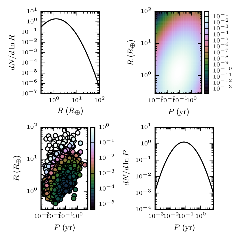
Figure 3.— The inferred planet period–radius distribution accounting for selection effects and false-positives. (Upper Left) The planet number density per logarithmic planet radius. The density peaks at $R_{\mathrm{peak}}=1.25_{-0.17}^{+0.16}R_{\oplus}$ (90% CL). (Upper Right) The planet number density in the period–radius plane. The inferred correlation coefficient between $\ln P$ and $\ln R$ is $r=0.334_{-0.053}^{+0.052}$. (Lower Left) Scatter plot of the radius and period of the Kepler planet candidates. Color indicates the posterior false-positive probability for each candidate. Overall, the model prefers a false-positive rate of $7.8_{-1.3}^{+1.4}\%$ (90% CL). The primary contaminant is probably background eclipsing binaries; our contamination rate is consistent with previous work (Fressin et al., 2013). (Lower Right) The planet number density per logarithmic planet period. The density peaks at $P=0.075_{-0.006}^{+0.007}\mathrm{yr}$ (90% CL).

Our model predicts a distribution for future observed data consistent with the already-observed candidate set. These predictions can be used to perform graphical and posterior-predictive model checking (Gelman et al., 2013). Fig. 4 compares the predictions of our model for observed periods and radii (incorporating both planetary transits and background events) with the candidate set. This is a particularly stringent test of our parameterised selection model since the observed periods and radii are strongly influenced by the selection function of the Kepler telescope and pipeline. Except for the known sub-population of hot Jupiters (Albrecht et al., 2012; Naoz et al., 2012), our model provides a very good fit to the observed data. That a simple log-normal distribution in period and radius fits the observed distribution of planets well may indicate that planet formation is a stochastic process with many small, correlated, and multiplicative influences on planet period and radius resulting, from the central limit theorem, in a log-normal distribution in these parameters.

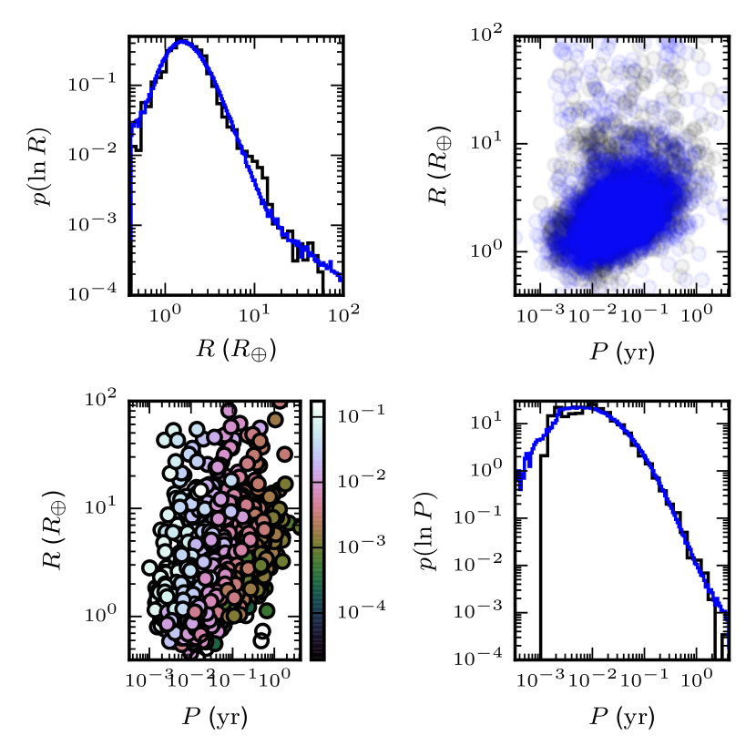
Figure 4.— Comparison of synthetic data sets produced from the forward model incorporating selection effects with observed candidates. (Upper Left) The observed (black curve) and synthetic (blue curve) normalised candidate density per logarithmic radius. Except for a discrepancy at $R\simeq 10R_{\oplus}$—associated with hot Jupiters, a distinct planetary population (Albrecht et al., 2012; Naoz et al., 2012)—the model produces a good fit to the observed candidates over the range of reported radii. Note particularly the tail at large radii that comes from background contaminants in both observed and synthetic data. (Upper Right) Scatter plot of the observed candidates (black circles) and a posterior-averaged draw of observed candidates from the model (blue circles). (Lower Left) Scatter plot of the observed candidates. Colors indicate the posterior-averaged selection probability for each planet about its host star (see Eq. (4)). (Lower Right) The observed (black curve) and synthetic (blue curve) normalised candidate density per logarithmic period. Except for the aforementioned hot Jupiter peak at $P\simeq 1\mathrm{day}$ the model produces a good fit to the observed candidates over the range of reported periods.

Previous estimates (Catanzarite & Shao, 2011; Traub, 2012; Dong & Zhu, 2013; Petigura et al., 2013; Foreman-Mackey et al., 2014) place $1\%\lesssim\eta_{\oplus}\lesssim 34\%$. These works dealt with the problem of selection effects in the sample by either analysing a region of the period-radius parameter space where observations are complete and extrapolating to $R=R_{\oplus}$ and $P=1\mathrm{yr}$ (Catanzarite & Shao, 2011; Traub, 2012), applying a binned analysis incorporating survey incompleteness in the period-radius plane (Dong & Zhu, 2013; Petigura et al., 2013) or analysing the results of a customised planet detection pipeline on a subset of the Kepler observations (Petigura et al., 2013; Foreman-Mackey et al., 2014). The methods and analysed data sets of Petigura et al. (2013); Foreman-Mackey et al. (2014) are most comparable to ours. These studies used the same data set, produced (Petigura et al., 2013) from a subset of the available Kepler data and a customised pipeline to search for transit signals. They both accounted for selection effects by measuring the recoverability of synthetic transit signals injected into their data, in contrast to our approach of empirically determining them from the observed data. Neither study attempted to account for contamination from falsely-identified candidate transit events, controlling this instead through careful choice of threshold. Both studies used a more flexible model for the intrinsic distribution of planets than ours. Our result for $\eta_{\oplus}$ is consistent with, but more precise than, Foreman-Mackey et al. (2014) and (somewhat) inconsistent with Petigura et al. (2013).

References

- Albrecht et al. (2012) Albrecht, S. et al. 2012, ApJ, 757, 18, arXiv:1206.6105
- Batalha et al. (2010) Batalha, N. M. et al. 2010, ApJ, 713, L109, arXiv:1001.0349
- Batalha et al. (2013) ——. 2013, ApJS, 204, 24, arXiv:1202.5852
- Borucki et al. (2010) Borucki, W. J. et al. 2010, Science, 327, 977
- Borucki et al. (2011) ——. 2011, ApJ, 736, 19, arXiv:1102.0541
- Brown et al. (2011) Brown, T. M., Latham, D. W., Everett, M. E., & Esquerdo, G. A. 2011, AJ, 142, 112, arXiv:1102.0342
- Catanzarite & Shao (2011) Catanzarite, J., & Shao, M. 2011, ApJ, 738, 151, arXiv:1103.1443
- Chatterjee et al. (2012) Chatterjee, S., Ford, E. B., Geller, A. M., & Rasio, F. A. 2012, MNRAS, 427, 1587, arXiv:1207.3545
- Christiansen et al. (2012) Christiansen, J. L. et al. 2012, PASP, 124, 1279, arXiv:1208.0595
- Dong & Zhu (2013) Dong, S., & Zhu, Z. 2013, ApJ, 778, 53, arXiv:1212.4853
- Duquennoy & Mayor (1991) Duquennoy, A., & Mayor, M. 1991, A&A, 248, 485
- Farr et al. (2013) Farr, W. M., Gair, J. R., Mandel, I., & Cutler, C. 2013, accepted by Phys. Rev. D, arXiv:1302.5341
- Foreman-Mackey et al. (2013) Foreman-Mackey, D., Hogg, D. W., Lang, D., & Goodman, J. 2013, PASP, 125, 306, arXiv:1202.3665
- Foreman-Mackey et al. (2014) Foreman-Mackey, D., Hogg, D. W., & Morton, T. D. 2014, ApJ, 795, 64, arXiv:1406.3020
- Fressin et al. (2013) Fressin, F. et al. 2013, ApJ, 766, 81, arXiv:1301.0842
- Gelman et al. (2013) Gelman, A., Carlin, J. B., Stern, H. S., Dunson, D. B., Vehtari, A., & Rubin, D. B. 2013, Bayesian Data Analysis, 3rd edn., Chapman & Hall/CRC Texts in Statistical Science (Chapman & Hall/CRC)
- Naoz et al. (2012) Naoz, S., Farr, W. M., & Rasio, F. A. 2012, ApJ, 754, L36, arXiv:1206.3529
- Petigura et al. (2013) Petigura, E. A., Howard, A. W., & Marcy, G. W. 2013, Proceedings of the National Academy of Science, 110, 19273, arXiv:1311.6806
- Tabachnik & Tremaine (2002) Tabachnik, S., & Tremaine, S. 2002, MNRAS, 335, 151, arXiv:astro-ph/0107482
- Traub (2012) Traub, W. A. 2012, ApJ, 745, 20, arXiv:1109.4682
- Weissbein et al. (2012) Weissbein, A., Steinberg, E., & Sari, R. 2012, ArXiv e-prints, arXiv:1203.6072
- Youdin (2011) Youdin, A. N. 2011, ApJ, 742, 38, arXiv:1105.1782