Constraints on the distribution and energetics of fast radio bursts using cosmological hydrodynamic simulations

Abstract

We present constraints on the origins of fast radio bursts (FRBs) using large cosmological simulations. We calculate contributions to FRB dispersion measures (DMs) from the Milky Way, from the local Universe, from cosmological large-scale structure, and from potential FRB host galaxies, and then compare these simulations to the DMs of observed FRBs. We find that the Milky Way contribution has previously been underestimated by a factor of $\sim 2$, and that the foreground-subtracted DMs are consistent with a cosmological origin, corresponding to a source population observable to a maximum redshift $z\sim 0.6-0.9$. We consider models for the spatial distribution of FRBs in which they are randomly distributed in the Universe, track the star-formation rate of their host galaxies, track total stellar mass, or require a central supermassive black hole. Current data do not discriminate between these possibilities, but the predicted DM distributions for different models will differ considerably once we begin detecting FRBs at higher DMs and higher redshifts. We additionally consider the distribution of FRB fluences, and show that the observations are consistent with FRBs being standard candles, each burst producing the same radiated isotropic energy. The data imply a constant isotropic burst energy of $\sim$$7\times 10^{40}$ erg if FRBs are embedded in host galaxies, or $\sim$$9\times 10^{40}$ erg if FRBs are randomly distributed. These energies are 10–100 times larger than had previously been inferred. Within the constraints of the available small sample of data, our analysis favours FRB mechanisms for which the isotropic radiated energy has a narrow distribution in excess of $10^{40}$ erg.

1 Introduction

Fast radio bursts (FRBs) are a newly identified and as-yet-unexplained class of transient objects (Lorimer et al., 2007; Thornton et al., 2013; Kulkarni et al., 2014). The ten known FRBs currently in the literature are characterised by short ($\approx 1$ ms), bright ($\ga$1 Jansky) bursts of radio emission; none have been seen to repeat, and all but two occurred at high Galactic latitude, $|b|>20^{\circ}$. The implied all-sky event rate is enormous, around 10 000 per day (Thornton et al., 2013).

The radio signals from FRBs experience a frequency-dependent dispersion delay as they propagate through ionised gas, just as is routinely seen for radio pulsars. However, for most observed FRBs, the very high dispersion measures (DMs), in the range 400–1100 pc cm^-3, are more than an order of magnitude larger than the DM contribution expected from the interstellar medium (ISM) of the Milky Way in these directions. The currently favoured interpretation is that the observed DMs seen for FRBs correspond primarily to free electrons in the intergalactic medium (IGM) along the line of sight (Luan & Goldreich, 2014; Dennison, 2014), with an additional but presumed small contribution from any host galaxy (Thornton et al., 2013). Simple assumptions about the density of the IGM then immediately imply that FRBs are at cosmological distances, corresponding to redshifts in the range 0.5–1 (Thornton et al., 2013).

The nature of FRBs is not known. Possibilities that have been proposed include flaring magnetars (Popov & Postnov, 2007, 2013; Lyubarsky, 2014), mergers of binary neutron stars (Totani, 2013), gamma-ray bursts (Zhang, 2014), collisions between neutron stars and asteroids/comets (Geng & Huang, 2015), or the collapse of supramassive neutron stars (“blitzars”; Falcke & Rezzolla, 2014). There are two approaches through which we can make further progress in discerning between these and other possibilities, One approach is to localise individual FRBs, so that we can then identify multi-wavelength counterparts, host galaxies, afterglows and redshifts. However, such data are not yet available, because all FRBs seen so far have been poorly localised, and most were not detected in the data until months or years after they were observed. The alternative is to consider the ensemble properties of FRBs, and to compare these to different simulated FRB distributions. In this paper we adopt the latter approach, in which we use state-of-the-art hydrodynamic simulations to consider synthesised populations of FRBs within a cosmological volume. We consider a series of simple assumptions as to the way in which FRBs are distributed relative to the distribution of large-scale structure, compute corresponding distributions of DM and fluence, and compare these to the observations. In §2 we summarise the observed properties of the ten published FRBs. In §3 we consider the various foreground contributions to the observed FRB DMs, including the Milky Way’s disk and spiral arms (§3.1), the Galactic halo (§3.2) and the local Universe (§3.3). In §4 we then calculate the expected cosmological component of FRB DMs using the Magneticum Pathfinder simulation, and compare this to observations. In §5 we compare simulated and observed FRB fluences in order to constrain the isotropic energy released in the radio bursts.

2 Observations of Fast Radio Bursts

The observational data we consider are the ten published FRBs as listed in Table 1, for each of which we provide Galactic coordinates, the observed value of DM, peak flux and fluence, and the central observing frequency at which the FRB was detected.

Table 1: Observed and derived properties of the ten published FRBs. The first seven columns list the observed parameters of each burst, as drawn from the references given in the eighth column. Note that Keane & Petroff (2015) provide revised peak fluxes and fluences for nine of the ten published FRBs, and further note that these revised values are further underestimates typically by a factor of $\sim 2$. In this Table, we have used the revised values of Keane & Petroff (2015) where available, and have further doubled all values of fluxes and fluences. DM_ISM, DM_halo and DM${}_{\rm local~{}sim}$ list the inferred contributions to the total DM from the Galactic disk and spiral arms (§3.1), Galactic halo (§3.2) and local Universe (§3.3), respectively. In the final column, DM_cosmo lists the dispersion measure contribution remaining after subtracting DM_ISM and DM_halo (but not DM${}_{\rm local~{}sim}$) from the observed value. As discussed in §3.3, we assume DM${}_{\rm LU}=0$ throughout.

FRB	$\ell$	$b$	DMobs	Peak flux	Fluence	Freq.	Ref.	DMISM	DMhalo	DM${}_{\rm local~{}sim}$	DMcosmo
	(∘)	(∘)	(pc cm-3)	(Jy)	(Jy ms)	(GHz)		(pc cm-3)	(pc cm-3)	(pc cm-3)	(pc cm-3)
0101251	356.6	–20.0	$790\pm 3$	1.10${}^{+0.22}_{-0.16}$	11.2${}^{+6.0}_{-4.0}$	1.4	1,2	110	30	13	650
010621	25.4	–4.0	$746\pm 1$	1.04${}^{+0.26}_{-0.22}$	8.6${}^{+7.2}_{-3.8}$	1.4	3,2	537	—	—	—
010724	300.8	–41.9	$375\pm 1$	$>3.16$	$>63.0$	1.4	4,2	44	30	20	301
110220	50.8	–54.7	$944.38\pm 0.05$	2.22${}^{+2.24}_{-0.20}$	14.6${}^{+4.8}_{-3.4}$	1.3	5,2	35	30	5	879
110626	355.8	–41.7	$723.0\pm 0.3$	1.26${}^{0.40}_{-0.26}$	1.8${}^{+2.6}_{-0.4}$	1.3	5,2	47	30	10	646
110703	81.0	–59.0	$1103.6\pm 0.7$	0.9${}^{+0.42}_{-0.20}$	3.6${}^{+4.6}_{-2.2}$	1.3	5,2	33	30	14	1041
120127	49.2	–66.2	$553.3\pm 0.3$	1.24${}^{+0.26}_{-0.20}$	1.6${}^{+1.2}_{-0.6}$	1.3	5,2	32	30	9	491
121102	175.0	–0.2	$557\pm 2$	0.8${}^{+0.8}_{-0.2}$	2.4${}^{+8.0}_{-2.0}$	1.4	6,2	192	30	10	335
131104	260.6	–21.9	$778.5^{+0.2}_{-0.3}$	2.2${}^{+0.1}_{-0.2}$	1.9${}^{+0.08}_{-0.18}$	1.4	7	71	30	10	678
140514	50.8	–54.6	$562.7\pm 0.6$	0.94${}^{+0.22}_{-0.16}$	2.6${}^{+4.6}_{-1.0}$	1.4	8,2	35	30	5	498

References: (1) Burke-Spolaor & Bannister (2014); (2) Keane & Petroff (2015); (3) Keane et al. (2012); (4) Lorimer et al. (2007); (5) Thornton et al. (2013); (6) Spitler et al. (2014); (7) Ravi et al. (2014); (8) Petroff et al. (2014a).

¹This burst was misnamed FRB 011025 by Burke-Spolaor & Bannister (2014).

3 Foreground Dispersion Measure

The DMs observed for FRBs as listed in Table 1 must consist of several contributions, corresponding to the various astrophysical structures through which the radio signal has traversed. For our purposes, the DM contributions both from the Milky Way Galaxy and from local large-scale structure are considered to be foregrounds, which we would like to remove to isolate the cosmological signal. Some of the foreground components are difficult to obtain from direct observations, and we use cosmological simulations to estimate the contribution of these components. We define the observed dispersion measure, DM_obs, as:

$${\rm DM}_{\mathrm{obs}}={\rm DM}_{\mathrm{ISM}}+{\rm DM}_{\mathrm{halo}}+{\rm DM}_{\mathrm{LU}}+{\rm DM}_{\mathrm{LSS}}+{\rm DM}_{\mathrm{host}},$$ (1)

where DM_ISM is the contribution from the Milky Way disk and spiral arms, DM_halo is that from the Galactic halo, DM_LU is that from the local Universe, DM_LSS is that from large-scale structure and DM_host is any contribution from any host galaxy or other immediate environment of the FRB. We define:

$${\rm DM}_{\rm cosmo}={\rm DM}_{\mathrm{LSS}}+{\rm DM}_{\mathrm{host}}$$ (2)

as the signal to be estimated from cosmological hydrodynamic simulations, with the remaining terms on the right-hand side of Equation (1) representing the foreground signal that must be accounted for in order to derive ${\rm DM}_{\rm cosmo}$ from DM_obs. Fig. 1 shows full sky-maps of the DM contributions of the various foreground components, as discussed in more detail in §§3.1, 3.2 and 3.3.

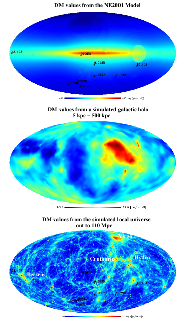
Figure 1: Full-sky maps of the DM contributions of various foregrounds, in Galactic coordinates centred on $\ell=0$, $b=0$. From top to bottom: DM_ISM predicted by the NE2001 model of Cordes & Lazio (2002, 2003); DM_halo contribution from a typical simulation of the extended halo of a Milky-Way-type galaxy; DM_LU contribution from the simulated local Universe out to a distance of 110 Mpc, showing prominent local large-scale structures such as the Perseus-Pisces region, the Virgo cluster and the Centaurus supercluster region. The positions of the FRBs in Table 1 are indicated in the top and bottom panels (FRB 140514 is at almost the same position as FRB 110220 and is not shown.)

3.1 The Galaxy Model

We calculate the foreground contribution from the Milky Way’s disk and spiral arms using the widely-used NE2001 distribution (Cordes & Lazio, 2002, 2003). This three-dimensional model of thermal electron density, $n_{e,{\rm NE2001}}$, is based on the DMs observed for Galactic radio pulsars, and includes contributions from axisymmetric thin and thick disks, Galactic spiral arms, and small-scale elements such as local under-dense regions and localised high density clumps.

We implement the NE2001 model using the hammurabi code (Waelkens et al., 2009) to integrate the Galactic electron density along a given sightline from the position of the Sun out to the limit of the model:

$$\mathrm{DM}_{\mathrm{ISM}}=\int_{0}^{\infty}n_{e,\mathrm{NE2001}}\,\mathrm{d}l~{}.$$ (3)

In Fig. 1 we show the full-sky DM signal for the NE2001 model, together with the positions of the FRBs in Table 1. We list our values derived for DM_ISM in Table 1 — the observed DMs far exceed DM_ISM except in the case of FRB 010621, where the two values are comparable. For this reason FRB 010621 has been argued to be of possible Galactic origin (Bannister & Madsen, 2014), and we exclude it from further consideration.

The estimates that we have derived for DM_ISM match the corresponding values given in the referenced papers, with the exception of FRB 010724 for which Lorimer et al. (2007) quoted DM${}_{\rm ISM}=25$ pc cm^-3 compared to DM${}_{\rm ISM}=44$ pc cm^-3 as given by NE2001 and listed here. We note that the NE2001 model is known not to give reliable estimates for pulsar distances or DMs at high Galactic latitudes, $|b|\ga 40^{\circ}$, as discussed extensively by Gaensler et al. (2008). However, this has minimal impact on our estimates of DM_ISM, which is integrated to the edge of the distribution. At high latitudes, the results of NE2001 can be roughly approximated as DM${}_{\rm ISM}\sim 30/|\sin b|$ pc cm^-3, while Gaensler et al. (2008) adopts DM${}_{\rm ISM}=26/|\sin b|$ pc cm^-3. The difference between these two options is typically $\la 1\%$ of DM_obs for FRBs.

3.2 The Halo Model

The values of DM_ISM calculated in §3.1 above only account for the foreground DM originating in the disk structure of the Milky Way; the NE2001 model lacks the contribution of a virialised dark matter halo with a hot gaseous atmosphere. As per Equation (1), we must also consider the free-electron contribution of the surrounding Galactic halo, which we model using numerical simulations. To estimate DM_halo, we use a cosmological simulation of a representative Milky Way-type galactic halo including hot thermal electrons. We use the existing simulations of Beck et al. (2013) to estimate the contribution to the DM. Fig. 1 shows an all-sky projection of the corresponding DM distribution.

The simulation of Beck et al. (2013) is based on initial conditions which were originally introduced by Stoehr et al. (2002). Briefly, the simulation is based on a large cosmological box with initial fluctuations of power spectrum index $n=1$ and a fluctuation amplitude $\sigma_{8}=0.9$, in which a Milky Way-like dark matter halo is identified. We use the fully magneto-hydrodynamic simulation labeled GA2, which contains 1,055,083 dark matter particles inside the virial radius at present redshift. The halo is comparable in mass ($\approx 3\times 10^{12}$ M_⊙) and in virial size ($\approx 270$ kpc) to the halo of the Milky Way. It does not undergo any major mergers after a redshift $z\approx 2$ and also hosts a sub-halo population comparable to the satellite population of our own Galaxy. Additionally, we follow the gas and stellar components by including multi-phase gas particles, which follow the prescriptions of radiative cooling, supernova feedback and star formation based on the work of Springel & Hernquist (2003a) but without galactic winds. Furthermore, the simulation is extended with magnetic fields following the implementation of Dolag & Stasyszyn (2009). In addition, Beck et al. (2013) further extend the original magnetohydrodynamic calculation of Beck et al. (2012) with a numerical sub-grid model for the self-consistent seeding of magnetic fields by supernova explosions.

The left panel of Fig. 2 shows some resulting predictions for radial electron density distributions representative of the Galactic halo, overplotted with observational data and constraints covering the entire virial radius, as presented by Miller & Bregman (2013), Grcevich & Putman (2009), Blitz & Robishaw (2000), Bregman & Lloyd-Davies (2007) and Gupta et al. (2012). Our simulated radial electron number density profile also agrees closely with the recent work of Nuza et al. (2014), which is based on a constrained simulation of the Local Group.

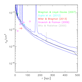
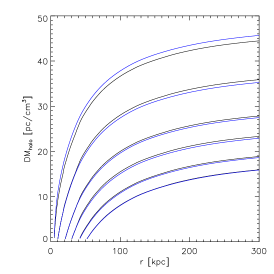
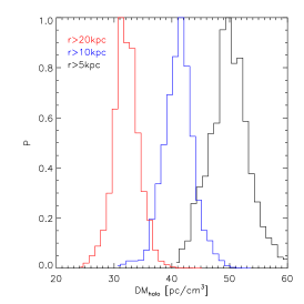
Figure 2: Predicted DM properties of a hot halo in a cosmological simulation of a Milky-Way-type galaxy. The left panel shows calculations for the radial distribution of free electrons, plus a comparison with observational constraints for the Milky Way. The black line shows the electron density obtained using the mean gas mass within each cell under the assumption of full ionisation of a primordial gas composition, while the blue lines show the median values, enveloped by the 10th and 90th percentiles of the electron density distribution within the simulation. The spikes in the simulated density profiles are caused by individual sub-structures within the simulated halo. The middle panel shows the corresponding integrated DM, the different lines indicating different inner radii used as the starting point for the integration. The right panel shows the predicted distribution of DM_halo over all possible sightlines, for three possible values of the inner radius.

The middle panel of Fig. 2 shows the cumulative increase of DM_halo as function of distance for different starting radii, while the right panel shows the distribution of DM_halo over all sightlines for these radii. At small radii, our results are consistent with the constraints from pulsar DMs discussed in §4.6 of Gaensler et al. (2008). Most interestingly, we find that the electrons in the hot Galactic halo make a non-negligible contribution to the total observed DMs for FRBs.

Our simulation of the halo has not been constrained to match the particular structure of the Milky Way, so we cannot calculate specific values of DM_halo for individual FRB sightlines as we did for DM_ISM in §3.1. Rather, we use the results of Fig. 2 to determine an indicative value for DM_halo. To make such an estimate, we should ideally use a radius to begin the integration that corresponds to the outer edge of the NE2001 model. However, this outer edge is direction-dependent and is not a well-defined concept. Given that the maximal extent of NE2001 from the Galactic centre is $\sim 17$ kpc (see Fig. 3 and Table 3 of Cordes & Lazio, 2002), we adopt from Fig. 2 a representative halo electron column DM${}_{\rm halo}=30$ pc cm^-3, as listed for all relevant FRBs in Table 1.

3.3 The Local Universe

To consider the possible contribution of local superclusters to the DMs observed for FRBs, we use the final output of a cosmological hydrodynamic simulation of the local Universe. Our initial conditions are similar to those adopted by Mathis et al. (2002) in their study (based on a pure N-body simulation) of structure formation in the local Universe. We first apply a gaussian smoothing to the galaxy distribution in the IRAS 1.2-Jy galaxy survey on a scale of 7 Mpc, and then evolve this structure linearly back in time back to $z=50$, following the method proposed by Kolatt et al. (1996). We then use the resulting field as a Gaussian constraint (Hoffman & Ribak, 1991) for an otherwise random realisation of a flat $\Lambda$CDM model, for which we assume a present matter density parameter $\Omega_{\mathrm{0m}}=0.3$, a Hubble constant $H_{0}=70$ km s^-1 Mpc^-1 and an root mean square (rms) density fluctuation $\sigma_{8}=0.9$. The volume constrained by the observational data covers a sphere of radius $\sim 110$ Mpc, centred on the Milky Way. This region is sampled with more than 50 million high-resolution dark matter particles and is embedded in a periodic box $\sim 343$ Mpc on a side. The region outside the constrained volume is filled with nearly 7 million low-resolution dark matter particles, allowing good coverage of long-range gravitational tidal forces.

Unlike in the original simulation of Mathis et al. (2002) where only the dark matter component was present, here we also follow the gas and stellar components. For this reason we extend the initial conditions by splitting the original high-resolution dark matter particles into gas and dark matter particles with masses of $m_{\mathrm{gas}}\approx 0.69\times 10^{9}$ M_⊙ and $m_{\mathrm{dm}}\approx 4.4\times 10^{9}$ M_⊙, respectively; this corresponds to a cosmological baryon fraction of 13 per cent. The total number of particles within the simulation is then slightly more than 108 million and the most massive clusters are resolved by almost one million particles. The physics included in the simulation is exactly the same as that used in the Magneticum Pathfinder simulation (to be described in §4.1 below). The lower panel of Fig. 1 shows the local structures and superclusters (Perseus-Pisces, Virgo and Centaurus are all prominent features) and the positions of the known FRBs. Table 1 lists DM${}_{\rm local~{}sim}$. for each FRB, defined as the DM contribution along each sightline from this Local Universe simulation. As can be seen, DM${}_{\rm local~{}sim}$ is relatively small in all cases, with none showing an excess that corresponds to any specific constrained structures. Since the sightlines are all through unconstrained regions, the values of DM${}_{\rm local~{}sim}$ have no specific significance, and are simply representative of the DM of low-contrast density enhancements in this local volume. The resulting dispersion from small-scale structure and the intergalactic medium is incorporated into the cosmological signal considered in §4, and we therefore assume henceforth that the specific contribution to DM from known structures in the Local Universe is DM${}_{\rm LU}=0$.

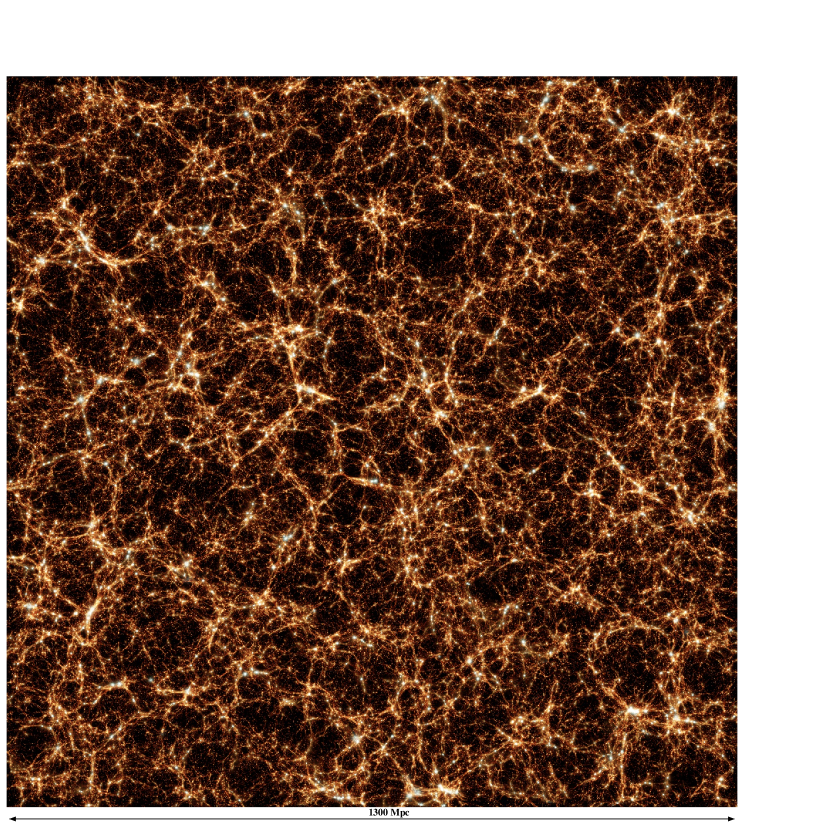
Figure 3: The distribution of baryonic material in the largest box of the Magneticum Pathfinder simulation at redshift zero. The colour indicates the gas temperature, ranging from dark red (cold) to light blue (hot), combined with the stellar component (white). The image shows a 100-Mpc thick, 1300-Mpc wide slice through the simulation at $z=0$.

4 Cosmological Dispersion Measure

After subtraction of the various foreground contributions to the DM as defined in Equation (1) and discussed throughout §3, the remaining excess dispersion is listed as DM_cosmo in Table 1. In all nine cases, this is by far the dominant contribution to the total observed DM.

Table 2: Properties of the two simulation runs from the Magneticum Pathfinder analysed in this study.

Name	Box size	Resolution level	Initial particle number	$m_{\mathrm{dm}}$	$m_{\mathrm{gas}}$	$m_{\mathrm{stars}}$	Softening length (dm, gas, stars)
	[Mpc/$h$]			[M${}_{\odot}/h$]	[M${}_{\odot}/h$]	[M${}_{\odot}/h$]	[kpc/$h$]
1300Mpc/mr	896	mr	$2\times 1,526^{3}$	$1.3\times 10^{10}$	$2.6\times 10^{9}$	$6.5\times 10^{8}$	10.0, 10.0, 5.0
500Mpc/hr	352	hr	$2\times 1,584^{3}$	$6.9\times 10^{8}$	$1.4\times 10^{8}$	$3.5\times 10^{7}$	3.75, 3.75, 2.0

In the following sections, we describe our derivation of DM_cosmo using hydrodynamic, cosmological simulations. As per Equation (2), this cosmological contribution to the DM of an FRB is composed of two parts. The first is DM_LSS, the signal coming from the diffuse gas within the cosmic web between the source and the observer. The second component is DM_host, the contribution from the host galaxy of the FRB. Here, due to limited spatial resolution, our simulations can only capture the hot atmosphere of virialised halos. For early-type galaxies, the host contribution should thus be incorporated by our simulation. However, for late-type galaxies, the simulation does not capture the contribution of the gas within the galactic disk. To properly model this component, additional assumptions or modeling would be required. For the purposes of the present discussion, we disregard the disk contribution to DM_host, because of the likely low inclination of the disk and because the $(1+z)^{-1}$ dilution of DM_host in the observer’s frame is larger than for all subsequently encountered dispersive media. (Thornton et al., 2013; McQuinn, 2014; Gao et al., 2014).

4.1 The Magneticum Pathfinder

We use the two largest simulations from the Magneticum Pathfinder data set (Dolag et al., in preparation). These two simulations use $896h^{-3}$ Mpc³ and $352h^{-3}$ Mpc³ boxes, simulated using $2\times 1526^{3}$ and $2\times 1584^{3}$ particles, respectively, where we adopt a WMAP7 (Komatsu et al., 2011) $\Lambda$CDM cosmology with $\sigma_{8}=0.809$, $h=0.704$, $\Omega_{m}=0.728$, $\Omega_{\Lambda}=0.272$, $\Omega_{b}=0.0456$, and an initial slope for the power spectrum of $n_{s}=0.963$. A visualisation of a 100-Mpc thick slice from the largest box at redshift $z=0$ is shown in Fig. 3. In Table 2 we summarise the details of the two simulations, including the dark matter particle mass, gas particle mass and softening length. Up to four stellar particles are generated for each gas particle.

Our simulations are based on the parallel cosmological TreePM-smoothed particle hydrodynamics (SPH) code P-GADGET3 (Springel, 2005). The code uses an entropy-conserving formulation of SPH (Springel & Hernquist, 2002) and follows the gas using a low-viscosity SPH scheme to properly track turbulence (Dolag et al., 2005b). It also allows radiative cooling, heating from a uniform time-dependent ultraviolet (UV) background, and star formation with the associated feedback processes. The latter is based on a sub-resolution model for the multi-phase structure of the ISM (Springel & Hernquist, 2003b).

Radiative cooling rates are computed through the procedure presented by Wiersma et al. (2009). We account for the presence of the cosmic microwave background (CMB) and for UV/X-ray background radiation from quasars and galaxies, as computed by Haardt & Madau (2001). The contributions to cooling from 11 elements (H, He, C, N, O, Ne, Mg, Si, S, Ca, Fe) have been pre-computed using the publicly available CLOUDY photoionisation code (Ferland et al., 1998) for an optically thin gas in (photo-)ionisation equilibrium.

In the multi-phase model for star formation (Springel & Hernquist, 2003b), the ISM is treated as a two-phase medium, in which clouds of cold gas form from the cooling of hot gas and are embedded in the hot gas phase. Pressure equilibrium is assumed whenever gas particles are above a given threshold density. The hot gas within the multi-phase model is heated by supernovae and can evaporate the cold clouds. Ten per cent of massive stars are assumed to explode as core-collapse supernovae (CCSNe). The energy released by CCSNe ($10^{51}$ erg per explosion) is modeled to trigger galactic winds with a mass loading rate proportional to the star-formation rate (SFR), to obtain a resulting wind velocity $v_{\mathrm{wind}}=350$ km s^-1. Our simulations also include a detailed model of chemical evolution (Tornatore et al., 2007). Metals are produced by CCSNe, by Type Ia supernovae and by intermediate and low-mass stars in the asymptotic giant branch (AGB). Metals and energy are released by stars of different mass by properly accounting for mass-dependent lifetimes (with a lifetime function as given by Padovani & Matteucci, 1993), the metallicity-dependent stellar yields of Woosley & Weaver (1995) for CCSNe, the yields of AGB stars from van den Hoek & Groenewegen (1997) and the yields of Type Ia supernovae from Thielemann et al. (2003). Stars of different mass are initially distributed according to a Chabrier (2003) initial mass function.

Most importantly, our simulations also include a prescription for black hole growth and for feedback from active galactic nuclei (AGN). As for star formation, accretion onto black holes and the associated feedback is tracked using a sub-resolution model. Supermassive black holes are represented by collisionless “sink particles” that can grow in mass either by accreting gas from their environments or by merging with other black holes. This treatment is based on the model presented by Springel et al. (2005) and Di Matteo et al. (2005) including the same modifications as in the study of Fabjan et al. (2010) plus some further adaptations (see Hirschmann et al., 2014, for a detailed description).

We use the SUBFIND algorithm (Springel et al., 2001; Dolag et al., 2009) to define halo and sub-halo properties. SUBFIND identifies sub-structures as locally overdense, gravitationally bound groups of particles. Starting with a halo identified through the Friends-of-Friends algorithm, a local density is estimated for each particle via adaptive kernel estimation, using a prescribed number of smoothing neighbours. Starting from isolated density peaks, additional particles are added in sequence of decreasing density. Whenever a saddle point in the global density field is reached that connects two disjoint overdense regions, the smaller structure is treated as a sub-structure candidate, and the two regions are then merged. All sub-structure candidates are subjected to an iterative unbinding procedure with a tree-based calculation of the potential. These structures can then be associated with galaxies, and their integrated properties (such as stellar mass or star-formation rate) can then be calculated. Note that with an adopted resolution limit for our simulations of $3\times 10^{9}$ M_⊙, any detected galaxy is assumed to contain a central supermassive black hole (SMBH).

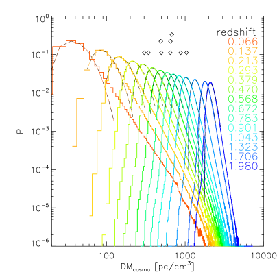
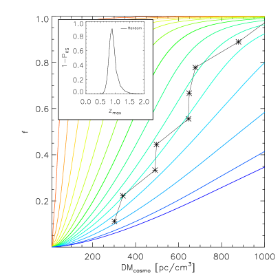
Figure 4: The expected distribution of DM_cosmo for FRBs derived from the medium-resolution simulation. The left panel shows histograms of DM_cosmo as a function of redshift from the 1300Mpc/mr simulation, with each coloured curve representing the distribution of DM_cosmo for a large ensemble of sightlines at a fixed redshift. Values of DM_cosmo observed for FRBs in Table 1 are shown by black diamonds. Fits to the simulated distributions of DM_cosmo are shown as black dashed lines (see text for details). The right panel shows cumulative distributions of DM_cosmo, obtained by integrating light-cones through the hydrodynamic simulation up to a maximum redshift $z_{\rm max}$, and assuming that FRBs are randomly distributed in the Universe — i.e., distributed randomly within the co-moving volume of every slice of the light-cone. Each coloured curve shows the cumulative distribution of DM_cosmo for a different redshift $z_{\rm max}$, using the same colours as in the left-hand panel. The black points show the corresponding cumulative distribution of DM_cosmo for FRBs from Table 1 (noting that DM_cosmo for FRB 110703 sits just outside the DM range plotted). The inset shows the probability derived from a KS test that the simulated and observed distributions of DM_cosmo could be drawn from the same underlying distribution, as a function of $z_{\rm max}$.

4.2 Calculating the Cosmological Dispersion Measure

Within the simulation we assume a primordial mixture of hydrogen and helium with a hydrogen mass fraction of 0.752, and when calculating the electron density we take into account the actual ionisation state of the medium. We disregard star-forming particles in this calculation, since their multi-phase nature means that their free electron density is not properly characterised. The cosmological frequency shift is taken into account when integrating the free electron density (McQuinn, 2014; Deng & Zhang, 2014), such that:

$$\mathrm{DM}_{\rm cosmo}(z_{\mathrm{max}})=\int_{0}^{z_{\mathrm{max}}}\frac{n_{e}(z)}{1+z}~{}dl,$$ (4)

where we integrate up to some maximum redshift of interest $z_{\mathrm{max}}$.

To actually construct past light-cones from the simulations, we follow the common approach to stack the co-moving volumes (e.g. placing them at the proper distance $w(z_{i})$) of the simulations (see for example Roncarelli et al. (2007); Ursino et al. (2010) for similar approaches). To avoid replications of similar structurs we randomized cosecutive slices by rotating and shifting. Our simulation volumes however are big enough so that we do not need to duplicate the simulation volumes for our 36 different individual slices. The number of outputs produced in the simulation was chosen so that the required radial integration length ($w(z_{i+0.5})-w(z_{i-0.5})$) of the individual slices always fit entirely within the simulated volume, which is placed at the proper distance $w(z_{i})$ according to the assumed cosmology. The opening angle is chosen so that the orthogonal extent — which depends on the angular diameter distance at the redshift of a slice – - always fits entirely within the simulated volume. The cosmological signal up to a maximum redshift $z_{\mathrm{max}}$ is thus approximated by the stacking of the individual slices:

$$\mathrm{DM}_{\rm cosmo}(z_{\mathrm{max}})=\sum_{i=0}^{i_{\rm max}}\int_{w(z_{i-0.5})}^{w(z_{i+0.5})}\frac{n_{e}(l)}{1+z_{i}}~{}dl.$$ (5)

We produce maps of the integrated electron density across each slice using SMAC (Dolag et al., 2005a), each resolved with $4096\times 4096$ pixels and covering a field of view of $13^{\circ}\times 13^{\circ}$ for the 1300Mpc/mr simulation and $5^{\circ}\times 5^{\circ}$ for the 500Mpc/hr simulation. Each of these slices represents the corresponding cosmological volume within the light-cone, while the actual integration is done converting the simulation to physical units first. We are using this volume, as well as the galaxies (and their properties) to weight the our source models as introduced in section §4.4.

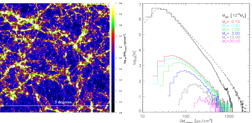
Figure 5: Results from the high-resolution simulation. The left-hand panel shows the distribution of DM_cosmo in the 500Mpc/hr simulation in a roughly 160-Mpc-thick slice of the light-cone at $z=0.5$; pink crosses mark the positions of the most massive galaxies. In the right-hand panel, we show the corresponding overall distribution function for DM_cosmo (black line), and the restricted distribution of DM_cosmo only at the positions of galaxies (coloured lines, with different colours showing differnet minimum thresholds for stellar massss). For comparison, the distribution of DM_cosmo for the lower-resolution but larger 1300Mpc/mr simulation is shown by a dashed line. With the exception of the tail at extreme DMs, the distributions of DM_cosmo in the two simulations are reasonably similar.

4.3 Medium-Resolution Simulation

We first consider results from the 1300Mpc/mr simulation, which covers a large cosmological volume at intermediate spatial resolution. This allows us to study the overall distribution of DM_cosmo down to the scale of galaxy groups. The resulting distribution of DM_cosmo as a function of $z_{\rm max}$ can be seen in the left panel of Fig. 4, where we show the distribution of DM_cosmo in the light-cone when integrating up to the indicated redshift. The nine observed values of DM_cosmo listed in Table 1 are shown as black diamonds in Fig. 4, confirming the conclusions of previous authors that FRBs occur at large cosmological distances, $0.5\la z\la 1$ (Ioka, 2003; Inoue, 2004; Lorimer et al., 2007; Thornton et al., 2013).

The dashed black lines shown in the left-hand panel of Fig. 4 indicate fits to the DM_cosmo distribution $P({\rm DM}_{\rm cosmo})$ of the form:

$$P({\rm DM}_{\rm cosmo})=A(z) \times \left[{\rm DM}_{\rm cosmo}+{\rm DM}_{00}(z)\right]^{2}$$ (6)

$$\times \mathrm{exp}\left(-\frac{{\rm DM}_{\rm como}+{\rm DM}_{01}(z)}{\sigma(z)}\right)$$

where the constants can be written as function of redshift,

$$A(z)=2\times 10^{-11}z^{-9}+1.3\times 10^{-7}z^{-4}+5\times 10^{-7}(z-2.325)^{2},$$ (7)

$${\rm DM}_{00}(z)=-770z^{1.3}+31.2\sqrt{z},$$ (8)

$${\rm DM}_{01}(z)=-108+926z+67z^{3},$$ (9)

$$\sigma(z)=126.9z+2.03-27.4z^{2}.$$ (10)

Note that we only fit the distribution of DM_cosmo down to 1% of the maximum value for each value of $z$, since this captures the bulk of the signal and because at their highest values the distributions of DM_cosmo take on a complex shape that can only be fit properly with a combination of several broken power laws. Note also that this tail toward large values of DM_cosmo is sensitive both to the largest supercluster structures present (and therefore to the size of the underlying cosmological simulation) and to the ability of the simulation to properly capture the inner regions and cool cores of galaxy clusters (see also the left panel of Fig. 5 and the associated discussion below).

The right-hand panel of Fig. 4 shows the expected cumulative distribution of DM_cosmo if the detected FRBs originate from random locations throughout the Universe (i.e., at a probability of incidence proportional to the co-moving volume within the light-cone) up to some maximum observable redshift $z_{\rm max}$. The observed cumulative distribution of DM_cosmo for FRBs, shown in black, closely matches the simulated distribution for $z_{\rm max}\sim 1$. We quantify this in the inset to the right-hand panel of Fig. 4, where we show the result of a series of Kolmogorov-Smirnoff (KS) tests between the observations and the simulated distributions as a function of $z_{\rm max}$. This demonstrates that the data only match the simulations in a narrow range around $z_{\rm max}\approx 0.9$.

We emphasise that although the 1300Mpc/mr simulation is currently the largest of its kind, the corresponding spatial resolution is not good enough to properly capture details in the halo structure (and especially precise stellar components of halos) at scales below massive galaxies. We therefore only use the 1300Mpc/mr simulation for the overall distribution of DM_cosmo (i.e., the component dominated by DM_LSS), a regime for which the 1300Mpc/mr simulation is superior to the higher-resolution 500Mpc/hr simulation because the former captures structures on much larger scales. We switch to the smaller, higher-resolution 500Mpc/hr simulation when stellar properties of the halos get important (e.g., when trying to account for DM_host), as we next consider in §4.4.

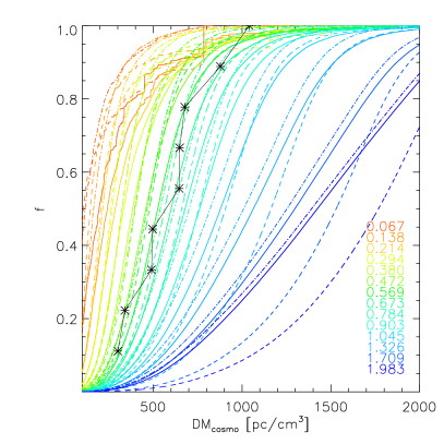
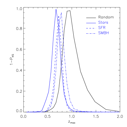
Figure 6: The expected cumulated distribution of DM_cosmo as a function of maximum observed FRB redshift, assuming that FRBs only occur in galaxies, and that the FRB rate for a given galaxy depends on stellar mass, (solid line), star-formation rate (dashed line) or the presence of a central SMBH (dash-dotted line). The left-hand panel shows the simulated cumulative distributions of DM_cosmo as a function of maximum redshift, $z_{\rm max}$, for these three models, with the observed distribution overlaid in black. The right-hand panel shows the results of KS tests between each model and the data, each as a function of $z_{\rm max}$.

4.4 High-Resolution Simulation

In §4.3, we used the medium-resolution 1300Mpc/mr simulation to determine the distribution of DM_cosmo for FRBs distributed randomly over the cosmic volume out to some maximum observable redshift. We now use the high-resolution 500Mpc/hr simulation to calculate the corresponding distribution of DM_cosmo when FRBs are embedded in potential host galaxies. We consider three simple models in which the spatial distribution of detectable FRBs within the simulation volume is correlated with the properties and locations of individual galaxies:

1. FRBs trace the total stellar component, as might result if FRBs are produced by an evolved population such as merging neutron stars. In this case, we assume that the FRB rate is proportional to the stellar mass within each galaxy. To compute the spatial distribution of FRBs, we only allow FRBs to occur at pixels in our simulation at which we identify a galaxy, and we weight the rate of FRB occurrence by the corresponding stellar mass.

2. FRBs are associated with massive stars, as would result if FRBs are produced by supernovae or young neutron stars. We here assume that the FRB rate is proportional to the current star-formation rate. We calculate the rate of FRBs by again only allowing an FRB to occur at a pixel associated with an individual galaxy, but we now weight the FRB rate by the current star-formation rate of that galaxy.

3. FRBs are associated with activity or interactions around the SMBH in a galaxy’s nucleus. Again we assume FRBs can only occur at pixels associated with individual galaxies, but we give all such pixels equal weight.

In each case, we wish to compute the expected distribution of DM_cosmo, and compare this to the FRB observations given in Table 1 to see if we can discriminate between possible FRB mechanisms. We construct simulated distributions of DM_cosmo by identifying the position of galaxies within each slice of the light-cone. The predicted value of DM_cosmo for an FRB occurring within a given galaxy (disregarding the disk contribution as discussed in §4) is then the contribution within the light-cone up to the position of that galaxy, as per Equation (4). Using the global properties of this galaxy determined as described in §4.1, we then assign a relative probability for the occurrence of an FRB at this location by weighting the correspondingly calculated value of DM_cosmo as per one of the three schemes described above.

The left-hand panel of Fig. 5 shows the contribution to DM_cosmo in the light-cone from a slice at redshift $z\approx 0.5$ in the 500Mpx/hr simulation, overplotted with the positions of the most massive galaxies (which correspond to the central galaxies in groups and clusters). The right-hand panel of Fig. 5 shows the distribution functions for DM_cosmo through all pixels in the full slice (black line) and only for pixels associated with galaxies above a threshold in stellar mass (colour coded). We also show the distribution of DM_cosmo for the same slice in the 1300Mpc/mr simulation (dashed line), in order to illustrate the contribution of even larger structures that are only present in the larger cosmological box. These large structures manifest as an excess in the tail of the distribution at the largest values of DM_cosmo. However, for the range in DM_cosmo corresponding to halos of all masses, the overall distributions of DM_cosmo for the medium- and high-resolution simulations are reasonably similar and the differences due to resolution and box size will not significantly alter any of our conclusions. In general, the range of values derived for DM_cosmo agrees with the estimates made by McQuinn (2014). Note that the different models for the spatial locations of FRBs all utilise the same underlying distributions in DM_cosmo, but give different weights to the individual pixels depending on the global properties of the galaxy associated with each pixel.

We perform this calculation for every slice of our light cone and thereby construct distributions of DM_cosmo as a function of $z_{\rm max}$ for each of the three different weighting schemes described above. The resulting cumulative distributions of DM_cosmo are shown in the left-hand panel of Fig. 6, together with the corresponding observed cumulative distribution of DM_cosmo for the FRBs listed in Table 1.

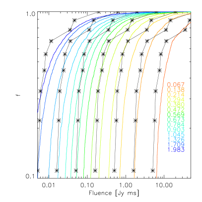
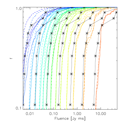
Figure 7: The expected distribution of FRB fluences as a function of maximum redshift, $z_{\rm max}$, assuming a nominal energy $E=1.4\times 10^{39}$ erg in the radio pulse. The left-hand panel shows simulations of the cumulative distribution of fluence as a function of maximum redshift for randomly distributed FRBs, while the right-hand panel shows the equivalent calculations when FRBs are associated with host galaxies and when the FRB rate depends on total stellar mass (solid line), star-formation rate (dashed line) or the presence of a central black hole (dotted line). The colours correspond to a range of maximum redshifts as per the legend to Fig. 4. Observed FRB fluences are overplotted in black: the second curve from the right shows the fluences in Table 1, while the other six curves show fluences shifted up or down in successive steps of half a decade to provide a scaling to other values of $E$.

There are only nine observed data points at present, collected in a very inhomogeneous way rather than from a single survey. Thus we cannot draw robust conclusions from the present sample. Nevertheless, the left-hand panel of Fig. 6 shows clearly that the detected FRBs extend up to a maximum redshift $z_{\rm max}\approx 0.6-0.9$, independent of their origin or detailed spatial distribution with respect to any host galaxies. We quantify this in the right-hand panel of Fig. 6, where we show the results of KS tests between the observed values of DM_cosmo and the simulated distributions as a function of maximum redshift for the three scenarios involving FRBs in host galaxies, and also for the random (unweighted) distribution of FRBs considered in §4.3. It is clear that all four possibilities are a reasonable match to the observations, although the best-fitting values of $z_{\rm max}$ are smaller for FRBs in host galaxies than for FRBs distributed randomly (as expected given that the former involves sightlines biased toward high DMs as per Fig. 5). The differences in the best fits for $z_{\rm max}$ for the three host-galaxy models are small, but the fact that case (i) gives a lower redshift than case (ii), and that case (ii) is lower than case (iii), can be understood qualitatively. If we adopt case (i) in which the frequency of FRBs tracks stellar mass, many sightlines to FRBs then involve high-mass systems, which therefore contribute more to DM_host and hence reduce the required value of $z_{\rm max}$. However, massive galaxies experience reduced star-formation due to SMBH activity in these systems; thus in case (ii), FRBs occur on sightlines to lower-mass galaxies, such that DM_host is lower and hence $z_{\rm max}$ is higher. Finally, FRBs associated with SMBHs result in a set of sightlines that have no weighting at all for the size of the host galaxy, and therefore result in even larger values of $z_{\rm max}$.

The similarities between the form of the cumulative DM_cosmo distributions of different weighting schemes at these redshifts (seen as the green curves in the left panel of Fig. 6) means that even once we obtain a much larger sample of FRBs, it will be difficult to use their DMs to discriminate between different possible origins if the observed values of DM_cosmo continue to mostly fall in the range $\sim 300-1000$ pc cm^-3. Conversely, as we approach $z_{\rm max}\sim 2$ the distributions of DM_cosmo diverge for the different weighting schemes (seen in blue in the left panel of Fig. 6). The much higher star-formation rate at these earlier epochs leads to larger differences in the weighting schemes between models, and thus to a broader range in the predicted distributions of DM_cosmo. If (through either improved sensitivity or simply a larger sample size) we can begin to detect an appreciable fraction of FRBs with DM${}_{\rm cosmo}\ga 1000-1500$ pc cm^-3, we may be able to distinguish between the different models, especially between FRB mechanisms that track the star-formation rate compared to other possibilities.

5 Expected Fluences and Energies

We now consider the implications for the observed distribution of FRB fluences. We consider the same three possible spatial distributions for FRBs as discussed in §4.4, along with a uniform (random) distribution of FRBs within the co-moving volume as in §4.3. However, while before we calculated distributions of DM from the simulations, here we infer fluences, and use these to test the hypothesis that FRBs are standard candles, each with the same emitted radio energy.

We assume that each FRB has the same isotropic total energy, $E$, where:

$$\frac{E}{4\pi D_{\mathrm{lum}}^{2}(z_{0})}=F_{\nu_{0}}~{}\nu_{0}(1+z_{0})~{},$$ (11)

for an FRB of received fluence $F_{\nu_{0}}$ at an observing frequency $\nu_{0}$, where $D_{\mathrm{lum}}$ is the luminosity distance for the FRB’s redshift, $z_{0}$.

Fig. 7 shows the expected cumulative distributions in fluences for a range of values of $E$ and as a function of maximum FRB redshift: the left panel shows how such fluences should be distributed if FRBs are located randomly in the cosmic volume (see §4.3), while the right panel shows the corresponding distribution if the number of FRBs per galaxy scales as the total stellar mass, as the star-formation rate, or at an equal rate per massive galaxy (see §4.4). For comparison, the cumulative distribution of observed fluences from Table 1 is overplotted as black points, and also shifted up or down to mimic different values of the fiducial energy that we assign to the FRBs. Again having only nine data points does not allow robust conclusions, but overall the shapes of the predicted distributions in fluence are all similar to that observed, showing that the data at present are consistent with the FRB population being standard candles. This favours mechanisms that produce FRBs through a deterministic process with a small number of free parameters (e.g., blitzars or neutron-star mergers; Totani, 2013; Falcke & Rezzolla, 2014) over stochastic process such as flares or reconnection events that typically show a wide distribution of energies (Popov & Postnov, 2013; Lyubarsky, 2014; Loeb et al., 2014). The fluences for a uniform (random) distribution show a very good agreement with the data. Models in which FRBs trace galaxies provide a slightly poorer match to the observed fluences, but this difference is not statistically significant, and none of the simulated distributions can be excluded. In Fig. 8 we show the value of the isotropic energy required to match the distribution of observed fluences as a function of maximum observed redshift, under the assumption that FRBs are standard candles, and for the same four models for the spatial distribution of FRBs as shown in Fig. 7. Note that this only depends on the spatial distribution of possible FRB hosts in the simulations. With the DM distributions considered in §§4.3 & 4.4, we can then infer $E\sim 7\times 10^{40}$ erg for any of the three models in which FRBs trace large-scale structure, for which we found $z_{\rm max}\sim 0.6-0.7$ in Fig. 6. For randomly distributed FRBs, for which we found $z_{\rm max}\approx 0.9$ in §4.3, $E$ is slightly larger than this ( $E\sim 9\times 10^{40}$ erg). We note that these energies, inferred using Equation (11), are 1–2 orders of magnitude larger than those reported in most other papers (e.g., Thornton et al., 2013; Keane & Petroff, 2015), because these previous authors have omitted the factor $4\pi$ needed to calculate isotropic energies, and have multiplied by the observing bandwidth rather than the observing frequency. The latter is far less dependent on the specifics of the observations, and (in the absence of any spectral index information) is a better rough estimate of the integrated radio energy of the burst; see §3.1 of Kulkarni et al. (2014) for a more detailed treatment. The energies we have calculated are a very good match to the predicted energy release $E\approx 3\times 10^{40}$ erg predicted by the blitzar model for FRBs presented by Falcke & Rezzolla (2014) and also agree with $E\ga 10^{40}$ erg expected from FRBs generated by magnetar flares (Lyubarsky, 2014; Kulkarni et al., 2014).

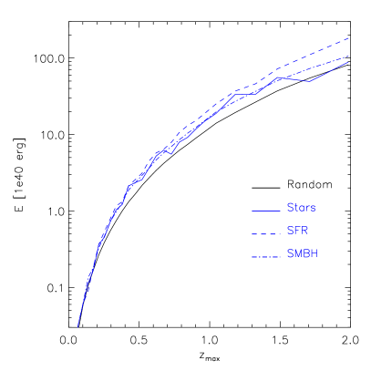
Figure 8: The isotropic FRB energy needed to match the observed distribution of cumulative fluences as a function of maximum redshift and for different models for the spatial distribution of FRBs, assuming all FRBs to be standard candles and using Equation (11) to convert between observed fluence and isotropic energy.

We note from Table 1 that FRBs 110220 and 140514 occurred at almost the same position on the sky, but with different DMs and different fluences. If FRBs are standard candles, the simplest expectation along a single sightline is that an FRB with a higher DM is farther away and thus must have a lower fluence. This is the opposite to what is observed for these two sources, for which FRB 140514 has a lower observed DM than FRB 110220 but also a lower fluence. However, given the significant angular structure seen in the simulation (see Fig. 5), we cannot exclude large fluctuations in DM, even along sightlines separated by 0.1 degrees. In addition, the reported fluences of FRBs have significant systematic uncertainties due to their unknown location within the telescope beam (see Spitler et al., 2014; Keane & Petroff, 2015).

6 Conclusions

We have used a set of advanced cosmological hydrodynamic simulations to investigate the contributions to dispersion measures of fast radio bursts from the Milky Way disk and halo, from the local Universe, from cosmological large-scale structure, and from potential host galaxies. Through this combination of calculations, we have made predictions for the expected DMs of FRBs distributed over different redshift ranges and for differing spatial distributions.

For the foreground (non-cosmological) contributions to DM, we obtain two main results:

1. The Milky Way’s hot halo contributes an additional $\sim$30 pc cm^-3 to the total DM, over and beyond the DM contribution from the Galactic disk predicted by the NE2001 model of Cordes & Lazio (2002, 2003). Except for FRBs at low Galactic latitudes ($|b|\la 20^{\circ}$), this means that the full Galactic contribution to FRM DMs is approximately double previous estimates.

2. By using a constrained simulation of the local Universe, we exclude any significant contribution to FRB DMs from prominent structures out to a distance of $\sim 110$ Mpc.

From our simulations of DMs at cosmological distances, we can make four additional conclusions:

1. The observed DM distribution for the available sample of nine extragalactic FRBs is consistent with a cosmological population detectable out to a redshift $z_{\rm max}\approx 0.6-0.9$, regardless of the specifics of how FRBs are distributed with respect to large-scale structure or the properties of their host galaxies.

2. If future observations can extend the FRB population to higher DMs and higher redshifts (DM${}_{\rm cosmo}\ga 1000-1500$ pc cm^-3, $z_{\rm max}\approx 2$) than for the currently known sample, we will be able to use the resulting DM distribution to determine whether FRBs are related to recent star formation or have some other origin.

3. The distribution of observed FRB fluences is consistent with a standard-candle model, in which the radio emission from each FRB corresponds to the same isotropic energy release.

4. Under the assumption that FRBs are standard candles, the isotropic energy associated with each radio burst is $\sim 7\times 10^{40}$ erg if FRBs are embedded in host galaxies and trace large-scale structure, or $\sim 9\times 10^{40}$ erg if FRBs occur at random locations in the Universe.

The blitzar model, in which a supramassive young neutron star is initially supported against gravitational collapse through its rapid rotation, but then later implodes to form a black hole once it has spin down sufficiently (Falcke & Rezzolla, 2014), is an FRB mechanism that may meet this joint requirement that FRBs are standard candles and that the radiated energy is $\ga 10^{40}$ erg. A more statistically robust distribution of fluences resulting from additional FRB detections will be able to better test whether FRBs are indeed standard candles, while an extension to higher redshifts can test whether FRBs track the star-formation rate as expected for the blitzar model.

There are many additional issues that we have not considered in this initial study. From an observational perspective, the fluxes and fluences of FRBs are difficult to determine (e.g., Spitler et al., 2014), and the selection effects associated with the detectability of FRBs are still being understood (Lorimer et al., 2013; Petroff et al., 2014b; Burke-Spolaor & Bannister, 2014; Keane & Petroff, 2015). In addition, DMs and fluences are not the only information available: most FRBs show significant scattering (e.g. Thornton et al., 2013), which in principle can provide additional constraints on their distances and environments (Macquart & Koay, 2013; Katz, 2014). In terms of foreground modeling, it is now well-established that the NE2001 model is not a complete description of the Galactic electron distribution, especially at high latitudes (Gaensler et al., 2008). While any errors in NE2001 do not have a qualitative effect on the conclusions of our present study, improved foreground electron distributions will be needed if FRBs are to be used as precision probes of cosmology and dark energy (e.g., Gao et al., 2014; Zhou et al., 2014). In addition, the exact distribution of baryons around galactic halos is still not well understood and depends on details of its implementation into numerical simulations (e.g. Ford et al., 2015), which could alter the DM signal expected from intervening, low mass galaxies (e.g. McQuinn, 2014). Looking to the future, not only can we expect larger numbers of FRBs, but we now know that FRBs are polarised (Petroff et al., 2014a). This raises the prospect of detecting Faraday rotation for FRBs, so that we can simultaneously obtain both DMs and rotation measures (RMs). Such data can provide direct measurements of the magnetisation of the IGM (Zheng et al., 2014; Macquart et al., 2015), and hence can potentially discriminate between different mechanisms for the origin of cosmic magnetism (e.g., Donnert et al., 2009).

References

- Bannister & Madsen (2014) Bannister, K. W. & Madsen, G. J. 2014, MNRAS, 440, 353
- Beck et al. (2013) Beck, A. M., Dolag, K., Lesch, H., & Kronberg, P. P. 2013, MNRAS, 435, 3575
- Beck et al. (2012) Beck, A. M., Lesch, H., Dolag, K., Kotarba, H., Geng, A., & Stasyszyn, F. A. 2012, MNRAS, 422, 2152
- Blitz & Robishaw (2000) Blitz, L. & Robishaw, T. 2000, ApJ, 541, 675
- Bregman & Lloyd-Davies (2007) Bregman, J. N. & Lloyd-Davies, E. J. 2007, ApJ, 669, 990
- Burke-Spolaor & Bannister (2014) Burke-Spolaor, S. & Bannister, K. W. 2014, ApJ, 792, 19
- Chabrier (2003) Chabrier, G. 2003, PASP, 115, 763
- Cordes & Lazio (2002) Cordes, J. M. & Lazio, T. J. W. 2002, arXiv:astro-ph/0207156
- Cordes & Lazio (2003) —. 2003, arXiv:astro-ph/0301598
- Deng & Zhang (2014) Deng, W. & Zhang, B. 2014, ApJ, 783, L35
- Dennison (2014) Dennison, B. 2014, MNRAS, 443, L11
- Di Matteo et al. (2005) Di Matteo, T., Springel, V., & Hernquist, L. 2005, Nature, 433, 604
- Dolag et al. (2009) Dolag, K., Borgani, S., Murante, G., & Springel, V. 2009, MNRAS, 399, 497
- Dolag et al. (2005a) Dolag, K., Hansen, F. K., Roncarelli, M., & Moscardini, L. 2005a, MNRAS, 363, 29
- Dolag & Stasyszyn (2009) Dolag, K. & Stasyszyn, F. 2009, MNRAS, 398, 1678
- Dolag et al. (2005b) Dolag, K., Vazza, F., Brunetti, G., & Tormen, G. 2005b, MNRAS, 364, 753
- Donnert et al. (2009) Donnert, J., Dolag, K., Lesch, H., & Müller, E. 2009, MNRAS, 392, 1008
- Fabjan et al. (2010) Fabjan, D., Borgani, S., Tornatore, L., Saro, A., Murante, G., & Dolag, K. 2010, MNRAS, 401, 1670
- Falcke & Rezzolla (2014) Falcke, H. & Rezzolla, L. 2014, A&A, 562, 137
- Ferland et al. (1998) Ferland, G. J., Korista, K. T., Verner, D. A., Ferguson, J. W., Kingdon, J. B., & Verner, E. M. 1998, PASP, 110, 761
- Ford et al. (2015) Ford, A. B., Werk, J. K., Dave, R., Tumlinson, J., Bordoloi, R., Katz, N., Kollmeier, J. A., Oppenheimer, B. D., Peeples, M. S., Prochaska, J. X., & Weinberg, D. H. 2015, ArXiv e-prints
- Gaensler et al. (2008) Gaensler, B. M., Madsen, G. J., Chatterjee, S., & Mao, S. A. 2008, PASA, 25, 184
- Gao et al. (2014) Gao, H., Li, Z., & Zhang, B. 2014, ApJ, 788, 189
- Geng & Huang (2015) Geng, J. J. & Huang, Y. F. 2015, ArXiv e-prints
- Grcevich & Putman (2009) Grcevich, J. & Putman, M. E. 2009, ApJ, 696, 385
- Gupta et al. (2012) Gupta, A., Mathur, S., Krongold, Y., Nicastro, F., & Galeazzi, M. 2012, ApJ, 756, L8
- Haardt & Madau (2001) Haardt, F. & Madau, P. 2001, in Clusters of Galaxies and the High Redshift Universe Observed in X-rays, ed. D. M. Neumann & J. T. V. Tran
- Hirschmann et al. (2014) Hirschmann, M., Dolag, K., Saro, A., Bachmann, L., Borgani, S., & Burkert, A. 2014, MNRAS, 442, 2304
- Hoffman & Ribak (1991) Hoffman, Y. & Ribak, E. 1991, ApJ, 380, L5
- Inoue (2004) Inoue, S. 2004, MNRAS, 348, 999
- Ioka (2003) Ioka, K. 2003, ApJ, 598, L79
- Katz (2014) Katz, J. I. 2014, 5766, arXiv:1409.5766
- Keane & Petroff (2015) Keane, E. F. & Petroff, E. 2015, MNRAS, 447, 2852
- Keane et al. (2012) Keane, E. F., Stappers, B. W., Kramer, M., & Lyne, A. G. 2012, MNRAS, 425, L71
- Kolatt et al. (1996) Kolatt, T., Dekel, A., Ganon, G., & Willick, J. A. 1996, ApJ, 458, 419
- Komatsu et al. (2011) Komatsu, E., Smith, K. M., Dunkley, J., Bennett, C. L., Gold, B., Hinshaw, G., Jarosik, N., Larson, D., Nolta, M. R., Page, L., Spergel, D. N., & Halpern, M. 2011, ApJS, 192, 18
- Kulkarni et al. (2014) Kulkarni, S. R., Ofek, E. O., Neill, J. D., Zheng, Z., & Juric, M. 2014, ApJ, 797, 70
- Loeb et al. (2014) Loeb, A., Shvartzvald, Y., & Maoz, D. 2014, MNRAS, 439, L46
- Lorimer et al. (2007) Lorimer, D. R., Bailes, M., McLaughlin, M. A., Narkevic, D. J., & Crawford, F. 2007, Science, 318, 777
- Lorimer et al. (2013) Lorimer, D. R., Karastergiou, A., McLaughlin, M. A., & Johnston, S. 2013, mnras, 436, L5
- Luan & Goldreich (2014) Luan, J. & Goldreich, P. 2014, ApJ, 785, L26
- Lyubarsky (2014) Lyubarsky, Y. 2014, MNRAS, 442, L9
- Macquart et al. (2015) Macquart, J.-P., Keane, E., Grainge, K., McQuinn, M., Fender, R. P., Hessels, J., Deller, A., Bhat, R., Breton, R., Chatterjee, S., Law, C., Lorimer, D., Ofek, E. O., Pietka, M., Spitler, L., Stappers, B., & Trott, C. 2015, ArXiv e-prints
- Macquart & Koay (2013) Macquart, J.-P. & Koay, J.-Y. 2013, ApJ, 776, 125
- Mathis et al. (2002) Mathis, H., Lemson, G., Springel, V., Kauffmann, G., White, S. D. M., Eldar, A., & Dekel, A. 2002, MNRAS, 333, 739
- McQuinn (2014) McQuinn, M. 2014, ApJ, 780, L33
- Miller & Bregman (2013) Miller, M. J. & Bregman, J. N. 2013, ApJ, 770, 118
- Nuza et al. (2014) Nuza, S. E., Parisi, F., Scannapieco, C., Richter, P., Gottlöber, S., & Steinmetz, M. 2014, MNRAS, 441, 2593
- Padovani & Matteucci (1993) Padovani, P. & Matteucci, F. 1993, ApJ, 416, 26
- Petroff et al. (2014a) Petroff, E., Bailes, M., Barr, E. D., Barsdell, B. R., Bhat, N. D. R., Bian, F., Burke-Spolaor, S., Caleb, M., Champion, D., Chandra, P., Da Costa, G., Delvaux, C., Flynn, C., Gehrels, N., Greiner, J., Jameson, A., Johnston, S., Kasliwal, M. M., Keane, E. F., Keller, S., Kocz, J., Kramer, M., Leloudas, G., Malesani, D., Mulchaey, J. S., Ng, C., Ofek, E. O., Perley, D. A., Possenti, A., Schmidt, B. P., Shen, Y., Stappers, B., Tisserand, P., van Straten, W., & Wolf, C. 2014a, MNRAS, in press (arXiv:1412.0342)
- Petroff et al. (2014b) Petroff, E., van Straten, W., Johnston, S., Bailes, M., Barr, E. D., Bates, S. D., Bhat, N. D. R., Burgay, M., Burke-Spolaor, S., Champion, D., Coster, P., Flynn, C., Keane, E. F., Keith, M. J., Kramer, M., Levin, L., Ng, C., Possenti, A., Stappers, B. W., Tiburzi, C., & Thornton, D. 2014b, ApJ, 789, L26
- Popov & Postnov (2007) Popov, S. B. & Postnov, K. A. 2007, arXiv:0710.2006
- Popov & Postnov (2013) —. 2013, arXiv:1307.4924
- Ravi et al. (2014) Ravi, V., Shannon, R. M., & Jameson, A. 2014, ApJ, in press (arXiv:1412.1599)
- Roncarelli et al. (2007) Roncarelli, M., Moscardini, L., Borgani, S., & Dolag, K. 2007, MNRAS, 378, 1259
- Spitler et al. (2014) Spitler, L. G., Cordes, J. M., Hessels, J. W. T., Lorimer, D. R., McLaughlin, M. A., Chatterjee, S., Crawford, F., Deneva, J. S., Kaspi, V. M., Wharton, R. S., Allen, B., Bogdanov, S., Brazier, A., Camilo, F., Venkataraman, A., Zhu, W. W., Aulbert, C., & Fehrmann, H. 2014, ApJ, 790, 101
- Springel (2005) Springel, V. 2005, MNRAS, 364, 1105
- Springel et al. (2005) Springel, V., Di Matteo, T., & Hernquist, L. 2005, MNRAS, 361, 776
- Springel & Hernquist (2002) Springel, V. & Hernquist, L. 2002, MNRAS, 333, 649
- Springel & Hernquist (2003a) —. 2003a, MNRAS, 339, 289
- Springel & Hernquist (2003b) —. 2003b, MNRAS, 339, 289
- Springel et al. (2001) Springel, V., White, S. D. M., Tormen, G., & Kauffmann, G. 2001, MNRAS, 328, 726
- Stoehr et al. (2002) Stoehr, F., White, S. D. M., Tormen, G., & Springel, V. 2002, MNRAS, 335, L84
- Thielemann et al. (2003) Thielemann, F.-K., Argast, D., Brachwitz, F., Hix, W. R., Höflich, P., Liebendörfer, M., Martinez-Pinedo, G., Mezzacappa, A., Panov, I., & Rauscher, T. 2003, Nuclear Physics A, 718, 139
- Thornton et al. (2013) Thornton, D., Stappers, B., Bailes, M., Barsdell, B., Bates, S., Bhat, N. D. R., Burgay, M., Burke-Spolaor, S., Champion, D. J., Coster, P., D’Amico, N., Jameson, A., Milia, S., Ng, C., Possenti, A., & van Straten, W. 2013, Science, 341, 53
- Tornatore et al. (2007) Tornatore, L., Borgani, S., Dolag, K., & Matteucci, F. 2007, MNRAS, 382, 1050
- Totani (2013) Totani, T. 2013, PASJ, 65, L12
- Ursino et al. (2010) Ursino, E., Galeazzi, M., & Roncarelli, M. 2010, ApJ, 721, 46
- van den Hoek & Groenewegen (1997) van den Hoek, L. B. & Groenewegen, M. A. T. 1997, A&AS, 123, 305
- Waelkens et al. (2009) Waelkens, A., Jaffe, T., Reinecke, M., Kitaura, F. S., & Enßlin, T. A. 2009, A&A, 495, 697
- Wiersma et al. (2009) Wiersma, R. P. C., Schaye, J., & Smith, B. D. 2009, MNRAS, 393, 99
- Woosley & Weaver (1995) Woosley, S. E. & Weaver, T. A. 1995, ApJS, 101, 181
- Zhang (2014) Zhang, B. 2014, ApJ, 780, L21
- Zheng et al. (2014) Zheng, Z., Ofek, E. O., Kulkarni, S. R., Neill, J. D., & Juric, M. 2014, ApJ, 797, 71
- Zhou et al. (2014) Zhou, B., Li, X., Wang, T., Fan, Y.-Z., & Wei, D.-M. 2014, Phys. Rev. D, 89, 107303