The Reionization of Carbon

Abstract

Observations suggest that $\mathrm{C\,II}$ was more abundant than $\mathrm{C\,IV}$ in the intergalactic medium towards the end of the hydrogen reionization epoch ($z\sim 6$). This transition provides a unique opportunity to study the enrichment history of intergalactic gas and the growth of the ionizing background (UVB) at early times. We study how carbon absorption evolves from $z=10$–5 using a cosmological hydrodynamic simulation that includes a self-consistent multifrequency UVB as well as a well-constrained model for galactic outflows to disperse metals. Our predicted UVB is within $\sim 2$–$4\times$ of that from Haardt & Madau (2012), which is fair agreement given the uncertainties. Nonetheless, we use a calibration in post-processing to account for Lyman-$\alpha$ forest measurements while preserving the predicted spectral slope and inhomogeneity. The UVB fluctuates spatially in such a way that it always exceeds the volume average in regions where metals are found. This implies both that a spatially-uniform UVB is a poor approximation and that metal absorption is not sensitive to the epoch when HII regions overlap globally even at column densites of $10^{12}$ cm^-2. We find, consistent with observations, that the $\mathrm{C\,II}$ mass fraction drops to low redshift while $\mathrm{C\,IV}$ rises owing the combined effects of a growing UVB and continued addition of carbon in low-density regions. This is mimicked in absorption statistics, which broadly agree with observations at $z=6$–3 while predicting that the absorber column density distributions rise steeply to the lowest observable columns. Our model reproduces the large observed scatter in the number of low-ionization absorbers per sightline, implying that the scatter does not indicate a partially-neutral Universe at $z\sim 6$.

1 Introduction

Intergalactic $\mathrm{C\,IV}$ and $\mathrm{C\,II}$ absorbers are observed along sightlines to quasars out to the highest redshifts probed (Songaila, 2001; Ryan-Weber et al., 2006; Becker et al., 2009; Ryan-Weber et al., 2009; Simcoe et al., 2011; D’Odorico et al., 2013; Becker et al., 2011). They occur naturally in cosmological hydrodynamic simulations in which galactic outflows expel metals out to the virial radius and beyond (Theuns et al., 2002; Cen et al., 2005; Oppenheimer & Davé, 2006; Oppenheimer & Davé, 2008; Oppenheimer et al., 2009; Cen & Chisari, 2011), opening up the possibility of using models to interpret them as tracers of star formation, outflows, and the ultraviolet ionizing background (UVB). $\mathrm{C\,IV}$ is the easier ion to observe owing to its larger oscillator strength and greater redshift separation from the Lyman-$\alpha$ forest. It is also relatively straightforward to model because it arises in gas that is optically thin to ionizing photons and lies far enough away from galaxies that the local radiation field may be neglected to first order. Its overall mass density is robustly observed to decline slowly with increasing redshift (Songaila, 2001; Becker et al., 2009; Ryan-Weber et al., 2009; D’Odorico et al., 2010, 2013; Simcoe et al., 2011; Becker et al., 2011; Cooksey et al., 2013). Numerous studies have shown that the observed decline can readily be accommodated by numerical simulations (Oppenheimer & Davé, 2006; Oppenheimer et al., 2009; Cen & Chisari, 2011). There remains some controversy as to what causes it: Some models indicate a combination of declining metallicity and increasing density (Oppenheimer & Davé, 2006; Oppenheimer et al., 2009) while others prefer an evolving mix of photoionization and shock-heating (Cen & Chisari, 2011). Future high-resolution observations of $\mathrm{C\,IV}$ absorbers past $z=3$ will constrain their velocity widths, which in turn can distinguish between different ionization mechanisms.

$\mathrm{C\,II}$ has received less theoretical and observational attention up until now. This is due to change as observations push into the hydrogen reionization epoch, where physical conditions favor increasingly neutral ionization states. For example,  Becker et al. (2011) have recently constrained the mass density of $\mathrm{C\,II}$, $\Omega_{\mathrm{C\,II}}$, to be $\geq 9\times 10^{-9}$ over the range $z=$5.3–6.4. For comparison, D’Odorico et al. (2013) find that $\Omega_{\mathrm{C\,IV}}$ is $8.4\times 10^{-9}$ over the interval $z=$5.30–6.20. Hence by $z=6$, $\mathrm{C\,IV}$ may already be subdominant to $\mathrm{C\,II}$. Note that correcting these measurements for incompleteness would strengthen the result: Becker et al. (2011) estimate that they are $>50\%$ complete for $\mathrm{C\,II}$ absorbers with column densities above $10^{13.5}$cm^-2, whereas D’Odorico et al. (2013) estimate 70% completeness for $\mathrm{C\,IV}$ absorbers stronger than $10^{13.4}$cm^-2. We will show (Figure 6) that $\mathrm{C\,II}$ is expected to become increasingly dominant to higher redshifts. Hence tracing the IGM metallicity into the reionization epoch essentially requires observations to shift from high- to low-ionization ions.

There is an additional reason to consider $\mathrm{C\,II}$ absorbers: At high redshift, $\mathrm{C\,II}$ traces lower-mass galaxies than $\mathrm{C\,IV}$ because only more massive galaxies can expel metals out to the low densities where $\mathrm{C\,IV}$ is the dominant ionization state; gas expelled by lower-mass galaxies remains at higher densities that favor $\mathrm{C\,II}$. In particular, Oppenheimer et al. (2009) (hereafter ODF09) find that $\mathrm{C\,II}$ absorbers at $z=6$ are associated with galaxies with stellar masses of $\sim 10^{7}M_{\odot}$ whereas $\mathrm{C\,IV}$ is seen near galaxies with $M_{*}\sim 10^{8}M_{\odot}$ (their Figures 21 and 23). The latter prediction is supported by observations that the two strongest $\mathrm{C\,IV}$ absorbers at $z\sim 6$ are physically associated with Lyman-$\alpha$ emitters (Díaz et al., 2014), whose stellar mass is characteristically $10^{8}$–$10^{10}M_{\odot}$ (Lidman et al., 2012). The tendency for low-ionization metal absorbers to trace predominantly lower-mass galaxies (Becker et al., 2011; Finlator et al., 2013; Kulkarni et al., 2013) immediately promotes them to a critical constraint on the origin of the UVB and of cosmological reionization because current models for reionization tend to rely heavily on low-mass galaxies to provide the required flux of ionizing photons (Finlator et al., 2011; Alvarez et al., 2012; Kuhlen & Faucher-Giguère, 2012; Jaacks et al., 2012; Robertson et al., 2013; Duffy et al., 2014; Wise et al., 2014). Such systems are generally too faint to be observed in emission, hence low-ionization absorbers will remain the only way to constrain their abundance for the foreseeable future.

These considerations motivate a closer look at the ionization state of carbon past $z=5$. How does the fraction of intergalactic carbon that is in $\mathrm{C\,II}$ and $\mathrm{C\,IV}$ evolve in time? How does this evolution map into absorption statistics? Does it contain the signature of reionization, or is the ionization state of carbon primarily determined by local sources? How many additional absorbers will be identified in future observations that probe to fainter column densities?

Modelling metal absorbers in the reionization epoch requires a treatment for the impact of local sources because the mean free path for ionizing photons drops below 10 proper Mpc for $z>5$ (Worseck et al., 2014). ODF09 explored the impact of a local field in a hydrodynamic simulation by assuming that each gas parcel’s ionization state is dominated by the closest galaxy’s radiation field (their Bubble model). They found that the local radiation field was much harder than the uniform Haardt & Madau (2001) UVB, leading broadly to more highly-ionized gas in which the $\mathrm{C\,II}$ and $\mathrm{C\,IV}$ column density distributions (CDDs) were respectively steeper and shallower. In particular, the predicted $\mathrm{C\,IV}$ CDD was found to vary with column $N_{\mathrm{C\,IV}}$ as $N_{\mathrm{C\,IV}}^{\alpha}$ with $\alpha=-1.4$ and -2.0 for their local field model versus the Haardt & Madau (2001) model. This result is quite intuitive: accounting for the fact that galaxies can amplify the UVB locally boosts the ionization parameter in outflowing gas, increasing the number of strong high-ionization systems at the expense of the low-ionization systems. Recently,  D’Odorico et al. (2013) measured the slope of the $\mathrm{C\,IV}$ CDD at $z\sim 6$ and found $\alpha=-1.7\pm 0.2$, favoring a somewhat flatter CDD (though not as flat as the Bubble model) and indicating a significant ionizing contribution from local sources. This model was therefore clearly a step in the right direction.

However, it neglected two important effects. First, galaxies are clustered such that, by $z=6$, an overdense gas parcel will be irradiated by many nearby galaxies rather than just the nearest one (Barkana & Loeb, 2004; Furlanetto et al., 2004a, b; Furlanetto & Oh, 2005). Second, gas that resides near galaxies is often dense enough to attenuate the weak reionization-epoch UVB before it reaches carbon atoms, boosting the predicted abundance of $\mathrm{C\,II}$. Working out which of these effects dominates requires improved theoretical models.

Recently, numerical simulations have acquired the ability to resolve the Jeans scale at the relevant redshifts while modeling the spatially-inhomogeneous UVB owing to stars and active galactic nuclei (AGN) self-consistently. These improvements remedy both of the problems mentioned above. In this paper, we use an updated model for the growth of structure and the UVB to study the ionization state of intergalactic carbon at $z\geq 5$. The outline of this work is as follows: In Section 2, we summarize our numerical model. In Section 3, we discuss our simulated UVB, compare it to the spatially-homogeneous Haardt & Madau (2012) model (hereafter HM12), and explain how we use the latter to calibrate our UVB. In Section 4, we compare the predicted $\mathrm{C\,II}$ and $\mathrm{C\,IV}$ fractions using our simulated UVB versus the HM12 UVB. In Section 5, we compare the predicted and observed absorber abundances. In Section 6, we then use the simulations to predict how the abundances of $\mathrm{C\,II}$ and $\mathrm{C\,IV}$ absorbers evolve in time. We also study the scatter in the number of absorbers per line of sight and produce predictions for the number of systems per survey. Finally, we summarize in Section 7.

2 Simulations

2.1 Hydrodynamics, Star Formation, and Feedback

Our simulation was run using a custom version of Gadget-3 (last described in Springel 2005). Hydrodynamics is modelled using a density-independent formulation of smoothed particle hydrodynamics (SPH) that treats fluid instabilities accurately (Hopkins, 2013). We compute the physical properties of each gas particle using a 5th-order B-spline kernel that incorporates information from up to 128 neighbours. Gas particles cool radiatively owing to collisional excitation of hydrogen and helium using the processes and rates in Table 1 of Katz et al. (1996), except that we relax the assumption of ionization equilibrium. We model metal-line cooling using the collisional ionization equilibrium tables of Sutherland & Dopita (1993).

Gas whose proper hydrogen number density exceeds 0.13 cm^-3 acquires a subgrid multiphase structure (Springel & Hernquist, 2003) and forms stars at a rate that is calibrated to match the observed Kennicutt-Schmidt law. We model metal enrichment owing to supernovae of Types II and Ia as well as asymptotic giant branch stars; see Oppenheimer & Davé (2008) for details. Galactic outflows form via a monte carlo model in which star-forming gas particles receive “kicks” in momentum space and are thereafter temporarily decoupled hydrodynamically. The outflow rates and velocities follow the “ezw” prescription introduced in Davé et al. (2013).

Our simulation discretizes the matter in a $6h^{-1}{\rm Mpc}$ volume using $2\times 256^{3}$ particles, which resolves the hydrogen-cooling limit at $10^{8}M_{\odot}$ with 65 particles. We generate the initial conditions using an Eisenstein & Hu (1999) power spectrum at $z=249$. We run the simulation to $z=3$, but we will focus mainly on results from snapshots taken at redshifts between 5 and 10. Our adopted cosmology is one in which $\Omega_{M}=0.3$, $\Omega_{\Lambda}=0.7$, $\Omega_{b}=0.045$, $h=0.7$, $\sigma_{8}=0.8$, and the index of the primordial power spectrum $n=0.96$.

2.2 Radiation Transport

We discretize the radiation field owing to galaxies spatially on a regular grid of $32^{3}$ voxels and spectrally into 16 frequency groups spaced evenly between 1–10 Ryd. Its evolution is followed via a moment method that couples with the opacity field from the gas in a way that captures the UVB’s feedback effect (Finlator et al., 2011). The emissivity of star-forming gas particles is proportional to their star formation rate, with a metallicity dependence that is computed from a modified version of Yggdrasil (Zackrisson et al., 2011). The emissivity is tabulated at 7 distinct metallicities between $Z=0$–$0.04$, and each gas particle’s actual emissivity is computed by interpolating to its $Z$. The $Z=0$ emissivity comes from Schaerer (2002); the $Z=10^{-5}$ and $Z=10^{-7}$ emissivities come from Raiter et al. (2010); and the $Z=0.001$–$0.040$ emissivities come from Starburst 99 (Leitherer et al., 1999), running with the Geneva tracks (high mass-loss version, without rotation) and Pauldrach/Hillier atmospheres. Each model is adjusted to a Kroupa IMF.

The most uncertain aspect of our model for the radiation field is the ionizing escape fraction from galaxies, $f_{\mathrm{esc}}$. Choosing a constant value for all masses and redshifts leads to a reionization history that either begins too late or overproduces the observed UVB amplitude at $z<6$ (Finlator et al., 2011; Kuhlen & Faucher-Giguère, 2012). In order to match both constraints, recent models assume that the volume-averaged $f_{\mathrm{esc}}$ varies in time (Kuhlen & Faucher-Giguère, 2012; Haardt & Madau, 2012; Mitra et al., 2013); this behavior is seen directly in some models (So et al., 2014). Alternatively, a number of detailed theoretical models suggest that $f_{\mathrm{esc}}$ is larger at lower masses (Wise & Cen, 2009; Yajima et al., 2011; Wise et al., 2014; Paardekooper et al., 2013; Ferrara & Loeb, 2013). Given that the typical mass of star-forming halos increases with time, this leads naturally to a scenario in which the mean $f_{\mathrm{esc}}$ decreases, yielding good agreement with observations (Alvarez et al., 2012).

We have found in practice that a pure mass dependence is not sufficient to match available constraints owing to the strong suppression of star formation by galactic outflows at low masses, so we adopt a model for $f_{\mathrm{esc}}$ that includes both mass- and redshift-dependence. We divide halos into three mass ranges. Minihalos ($M_{h}\leq 10^{8}M_{\odot}$) have $f_{\mathrm{esc}}=0.8$ at all times. Photoresistant halos ($M_{h}\geq 10^{9.5}M_{\odot}$) have an $f_{\mathrm{esc}}$ that varies with redshift:

$$f_{\mathrm{esc}}=\left\{\begin{array}[]{lc}0.5&z\geq 10\\ f_{\mathrm{esc,5}}\left(\frac{1+z}{6}\right)^{\kappa}&z<10\end{array}\right.$$ (3)

Here, the $f_{\mathrm{esc}}$ from photoresistant halos at $z=5$ is $f_{\mathrm{esc,5}}=0.05$ and the slope of the redshift dependence is $\kappa=3.8$. The $f_{\mathrm{esc}}$ from photosensitive halos ($10^{8}<M_{h}/M_{\odot}<10^{9.5}$) varies linearly with $\log(M_{h}/M_{\odot})$ between 0.8 at $10^{8}M_{\odot}$ and the redshift-dependent value for photoresistant halos. This model associates high $f_{\mathrm{esc}}$ values with lower masses and earlier times.

Note that, in our model, $f_{\mathrm{esc}}$ does not depend on frequency. This contrasts with HM12, who assume that no photons with energies above 4 Ryd escape from galaxies. Our choice is motivated by theoretical models in which ionizing radiation escapes either by leaking through porous ISMs or because some stars have irregular orbits that take them outside the ISM’s dense regions (Wise & Cen, 2009). In both scenarios, the wavelength dependence of $f_{\mathrm{esc}}$ could be weak. In practice, however, we have verified that this assumption has negligible impact on our predictions regarding $\mathrm{C\,IV}$ and $\mathrm{C\,II}$ absorbers at $z\sim 6$, hence we will not discuss it further.

We model the AGN radiation field via a spatially-averaged radiation transfer calculation (see equation 1 of HM12). The field is discretized spectrally into the same frequency bins as the galaxy field but is spatially uniform (except in dense regions, where it is attenuated by a self-shielding model that we describe below). The emissivity and spectral shape are taken from Equations 37 and 38 of HM12, with the modification that the emissivity vanishes at $z>8$ (this assumption does not matter because galaxies dominate the UVB at energies less than 10 Ryd for $z>4$). The sink term is given by the simulation’s volume-averaged opacity. The transfer calculation is included in the simulation’s cooling/ionization iteration, hence it is fully coupled into the radiation hydrodynamic framework.

The radiation field is not modelled with high enough spatial resolution to capture self-shielding in Lyman limit systems, hence we attenuate it in dense regions using a subgrid prescription based on the local Jeans length that is a generalization of the model presented in Schaye (2001). This model is not important for $\mathrm{C\,IV}$ absorbers as they arise primarily in the circumgalactic medium. On the other hand, it is crucial for low-ionization absorbers (Figure 1 of Finlator et al., 2013), which arise in denser gas.

The optical depth $\tau_{\nu}$ through a region in hydrostatic equilibrium with Jeans length $L_{\mathrm{J}}$ owing to a set of species $n_{i}$ with absorption cross sections $\sigma_{\nu,i}$ is given by

$$\tau_{\nu}=L_{\mathrm{J}}\sum_{i}n_{i}\sigma_{\nu,i},$$ (4)

where we sum only over the abundances of neutral hydrogen and neutral and singly-ionized helium. To compute the local ion abundances $n_{i}$, we assume that gas is in photoionization equilibrium (note that this assumption is only used to model self-shielding; the actual ionization states of hydrogen and helium are tracked using our nonequilibrium ionization solver). Following HM12, we define the following dimensionless ionization parameters:

$$R_{\mathrm{HI}} = \frac{\Gamma_{\mathrm{HI}}}{n_{e}\alpha_{\mathrm{HII}}}$$

$$R_{\mathrm{HeI}} = \frac{\Gamma_{\mathrm{HeI}}}{n_{e}\alpha_{\mathrm{HeII}}}$$

$$R_{\mathrm{HeII}} = \frac{\Gamma_{\mathrm{HeII}}}{n_{e}\alpha_{\mathrm{HeIII}}}$$

With these definitions, Equation 4 may be expanded to

$$\begin{aligned} \tau_{\nu}=&L_{\mathrm{J}}n_{H}\times\\ &\left[\frac{\sigma_{\nu,HI}}{(1+R_{\mathrm{HI}})}+\frac{1-X_{H}}{4X_{H}}\frac{(\sigma_{\nu,HeII}+R_{\mathrm{HeI}}\sigma_{\nu,HeIII})}{(1+R_{\mathrm{HeI}}+R_{\mathrm{HeI}}R_{\mathrm{HeII}})}\right].\end{aligned}$$ (5)

In order to evaluate equation 5, we need the photoionization rates $\Gamma_{i}$, gas temperature, and electron abundance. We adopt the local values for each particle, all of which are computed self-consistently by the simulation. In Appendix A, we show that this treatment is in good agreement with the spatially-resolved radiation transport calculations of Rahmati et al. (2013).

Although our simulation volume is too small to be numerically resolved, it yields a plausible reionization history. The bottom panel of Figure 1 shows the time-evolution of the volume-averaged neutral fraction $x_{\mathrm{H\,I,V}}(z)$. The predicted reionization history is extended, with $x_{\mathrm{H\,I,V}}$ dropping below 90% at $z\sim 10$ and 50% shortly after $z=8$. The predicted optical depth to Thomson scattering $\tau_{\mathrm{es}}$ is 0.057, which is barely within the observed $2\sigma$ confidence interval of $0.081\pm 0.012$ (Hinshaw et al., 2013). This value is considerably lower than our previous simulation, which yielded 0.071 (Finlator et al., 2013). The difference owes to varying degrees to the lower adopted values for $\sigma_{8}$ and $\Omega_{b}$ (0.08 and 0.045 versus 0.082 and 0.046, respectively); our smaller cosmological volume (our current simulation volume subtends 6 versus 9$h^{-1}{\rm Mpc}$); and our different model for the ionizing escape fraction, which is capped at 0.8 rather than 1.0 and decreases to high masses rather than being constant at all masses. Additionally, the ezw outflow model suppresses star formation in halos with circular velocities below 75$\;{\rm km}\,{\rm s}^{-1}$ more strongly than the previous vzw model (Davé et al., 2013), delaying the early stages of reionization. In short, the differences between our previous and current simulations generally delay the current model’s reionization and suppress $\tau_{\mathrm{es}}$. This reinforces the well-known problem that reionization via galaxy formation, while possible within the concordance cosmology, is challenging.

Despite the somewhat delayed reionization history, we believe that our model gives a plausible representation model for the UVB and metal absorbers during the latter stages of the reionization epoch for two reasons. First, the volume-averaged neutral hydrogen fraction drops below 1% at $z=6.5$. This is reasonably consistent with the observation that it is very small ($<10^{-3}$) by $z=6$ (Fan et al., 2006; Becker et al., 2014), although large-scale fluctuations in the UVB may remain until $z=5$ (Schroeder et al., 2013; Becker et al., 2014; Malloy & Lidz, 2014). Furthermore, we will show in Figure 2 that the simulated Lyman-$\alpha$ forest optical depth is either at the lower or upper end of the observed range, depending on our treatment of the UVB. Hence although the model may not account for all ionizing sources at $z\geq 10$, we expect that it does at later epochs. Second, our mass resolution is higher than the w8n256 simulation discussed by Oppenheimer & Davé (2006), which was already shown to yield converged predictions for absorbers down to columns of $10^{12}$cm^-2. This indicates our simulation fully accounts for the galaxy population that generates low-column absorbers.

3 The Simulated Radiation Field

In this section, we discuss our simulated radiation field. Our model predicts that $\mathrm{C\,IV}$ absorbers are photoionization-dominated because gravitational and outflow-driven shocks do not heat enough enriched gas to the temperatures at which $\mathrm{C\,III}$ can be collisionally ionized (ODF09). This is consistent with the observational result that, at $z\sim 3$, $\mathrm{C\,IV}$ absorbers in high-resolution spectra have narrow velocity widths implying an origin in photoionization (Prochaska & Wolfe, 1997; Tescari et al., 2011).

At $z>3$, Cen & Chisari (2011) predict a transition from photoionization to collisional ionization of $\mathrm{C\,IV}$-absorbing gas. Unfortunately, observations of $\mathrm{C\,IV}$ absorbers at these redshifts cannot yet test whether they consist of multiple narrow ($b$-parameters $<25\;{\rm km}\,{\rm s}^{-1}$) components, which is necessary to rule out the collisional ionization hypothesis. At $z\sim 6$, Becker et al. (2011) use high-resolution spectra of seven low-ionization absorbers to find velocity widths of 10–100$\;{\rm km}\,{\rm s}^{-1}$ (Becker et al., 2011). Four of these have velocity widths $\leq 25\;{\rm km}\,{\rm s}^{-1}$, indicating negligible collisional ionization of CIII. The other three have widths of up to $200\;{\rm km}\,{\rm s}^{-1}$. Such broad widths indicate sufficiently energetic gas to collisionally ionize metals completely. Remarkably, however, even these systems are undetected in $\mathrm{C\,IV}$ and $\mathrm{Si\,IV}$ (with the possible exception of a weak $\mathrm{C\,IV}$ system at $z=5.79$ in the spectrum of SDSS J0818+1722), hence the presence of low-ionization systems may indicate turbulent broadening of cold gas. One of their quasars (SDSS J1030+0524) does contain coincident $\mathrm{C\,II}$ and $\mathrm{C\,IV}$ absorption at $z=5.7425$, but this is only seen in the X-shooter spectrum of D’Odorico et al. (2013), where the data quality do not permit a robust constraint on its $b$-parameter. More high-resolution data will be required to test the hypothesis that $\mathrm{C\,IV}$ is collisionally-ionized at $z>3$.

In short, an origin in photoionization remains consistent with available constraints at $z\geq 3$. For the present, we therefore persist in the simple approach of asking how well our current simulation performs and speculate for the purposes of future work as to how important the subgrid scales are.

3.1 Amplitude

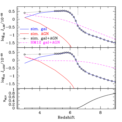
Figure 1: The amplitude of the ionizing background in ergs s^-1 cm^-2 Hz^-1 Sr^-1 at the ionizing edges of $\mathrm{H\,I}$ (top) and $\mathrm{C\,III}$ (middle). Red and blue solid curves show the contributions from galaxies and AGN, while the black dotted curve gives their total. The dashed curve is from HM12, smoothed to the same spectral resolution as our simulation. The bottom panel shows the volume-averaged neutral hydrogen fraction $x_{\mathrm{H\,I,V}}$, while the vertical sements in the top and middle panels indicate where $x_{\mathrm{H\,I,V}}$ drops below 1%. The simulated radiation field’s amplitude is 2–3$\times$ larger than in the HM12 model throughout the observed epoch and is dominated by galaxies rather than AGN.

In Figure 1, we show how the simulated UVB’s amplitude at the $\mathrm{H\,I}$ and $\mathrm{C\,III}$ ionization edges evolves with time. For comparison, we also show the volume-averaged neutral hydrogen fraction in the bottom panel. Prior to the completion of hydrogen reionization, the volume-averaged UVB grows smoothly as the mean free path to ionizing photons increases. Its amplitude then jumps when reionization completes ($z=6.5$). This is a well-known numerical artefact of computing reionization in small volumes (Barkana & Loeb, 2004; Iliev et al., 2014), and owes to an overly-rapid increase in the mean free path of ionizing photons.

Following reionization, the contribution from galaxies to the UVB declines slowly while the contribution from AGN increases more rapidly. The combination of the two yields a nearly invariant UVB amplitude, in qualitative agreement with observations (Becker & Bolton, 2013). To our knowledge, this represents the first attempt to model both the pre- and post-reionization UVB in a three-dimensional framework. The fact that, despite its limitations, our model already reproduces the UVB’s observed non-evolution is an encouraging victory.

For reference, we also show the UVB amplitude predicted by the HM12 model. For a fair comparison with our simulation’s low spectral resolution, we average the HM12 model over the energy range 1.0–1.5625 Ryd in the top panel and 3.25–3.8125 Ryd in the middle panel. The simulated background lies below the HM12 model prior to reionization, but this is not a serious problem as the latter is a volume-averaged calculation that becomes inaccurate in epochs where the UVB becomes highly inhomogeneous. Following reionization, the simulated UVB is 2–4$\times$ stronger than the HM12 model, with the gap declining to $z=3$. This discrepancy is not large compared to the observational uncertainties, which characteristically span a factor of 2–3 (Becker & Bolton, 2013). Moreover, it is difficult to avoid in numerical simulations because the UVB amplitude $J$ varies with the ionizing emissivity $\epsilon$ as $J\propto\epsilon^{3}$–$\epsilon^{4}$ (McQuinn et al., 2011). As long as galaxies dominate the UVB, $\epsilon\propto f_{\mathrm{esc}}$, so a factor of three in $J$ translates to a factor of $<1.5$ in $f_{\mathrm{esc,5}}$. This nonlinear dependence, combined with the high computational expense of radiation transport simulations, means that “hitting the target” is very challenging. For the present, we simply adjust our simulated UVB by a factor $J_{\rm{HM12}}/\langle J_{\rm{sim}}\rangle$ (where the amplitudes are evaluated at the $\mathrm{H\,I}$ ionization edge) wherever it overproduces the HM12 model. This calibration preserves the simulated UVB’s shape and spatial inhomogeneity below $z=6.5$ and leaves it entirely unchanged at earlier times. In what follows, we will refer to this UVB as the “renormalized” one as compared to the directly-computed, “simulated” one.

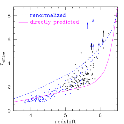
Figure 2: The volume-averaged optical depth to aborption by the Lyman-$\alpha$ forest as a function of redshift directly predicted by the simulation (solid magenta) and under the assumption of ionization equilibrium with the renormalized UVB (dashed blue). The two curves broadly bracket the observed range at $z>5$ while the simulated curve is in excellent agreement with observations at later times. Black circles and blue squares are from Fan et al. (2006) and Becker et al. (2014), respectively, while arrows indicate regions where no transmission was detected at $2\sigma$.

In order to examine to what extent the simulated and renormalized UVBs agree with IGM observations, we have computed the volume-averaged optical depth to absorption by the Lyman-$\alpha$ forest $\tau_{\mathrm{Ly}\alpha}$ in both cases. The solid magenta curve in Figure 2 shows the simulated optical depth. It is in remarkably good agreement with observations for $z<5$ (Fan et al., 2006; Becker et al., 2014). From $z=5$–5.8, it traces the lower end of the observed range, indicating that it is slightly too strong. Above $z=5.8$, it is much stronger than implied by observations.

These discrepancies can be traced to two factors. First, the tendency for the simulated $\tau_{\mathrm{Ly}\alpha}$ to evolve too quickly is a well-known artefact of small volumes (Barkana & Loeb, 2004; Iliev et al., 2014) that will improve through increased dynamic range. Second, the Lyman-$\alpha$ forest is increasingly sensitive to rare voids at high redshifts (Bolton & Becker, 2009); these are systematically absent from small volumes. Note that, by contrast, metal absorbers are likely weighted toward overdense regions where galaxies form. In other words, our simulation probably yields a better model for metal absorbers than for the Lyman-$\alpha$ forest.

In order to produce the blue dashed curve corresponding to the renormalized UVB, we recomputed each gas particle’s ionization state under the assumption of ionization equilibrium given the local temperature and density (this introduces $\sim 1\%$ shifts in $\tau_{\mathrm{Ly}\alpha}$ with respect to a full non-equilibrium calculation). The renormalized UVB traces the upper envelope of the observed range from $z=5-6$. This is consistent with the view that our simulation lacks large-scale voids where the gas would be on average more ionized (Bolton & Becker, 2009). Expanding our dynamic range would suppress $\tau_{\mathrm{Ly}\alpha}$ into improved agreement with observations.

While Figure 2 does not obviously favour one UVB model over the other, we will find it convenient to assume the renormalized UVB in order to facilite comparisons with the HM12 model. At the same time, in Section 5 we will leverage the fact that the simulated and renormalized UVBs bracket observations to explore the impact of UVB fluctuations on length scales that our simulation does not capture.

3.2 Spectral Slope

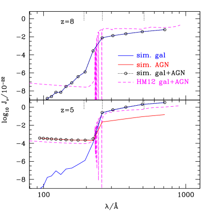
Figure 3: The simulated UVB from 1–10 Ryd at two representative redshifts along with the HM12 model. Dotted vertical ticks indicate the ionization potentials of $\mathrm{C\,II}$, $\mathrm{C\,III}$, and $\mathrm{C\,IV}$. Note that our model does not account for the sawtooth opacity of singly-ionized helium owing to its low spectral resolution.

We show in Figure 3 how galaxies and AGN contribute to the total UVB at two representative redshifts and compare with the HM12 model. Note that these figures do not include the calibration discussed in Section 3.1. This comparison reveals two differences in addition to the small amplitude offset discussed in Section 3.1. First, we note that, redwards of the HeII ionization edge (228 Å), the simulated background is redder at $z=8$ than in the HM12 model. This discrepancy cannot owe to the metallicity of the star-forming gas because the simulation’s star formation-rate weighted mean metallicity is roughly 0.5–0.6 times as large as assumed by HM12 (their equation 52) for $z=6$–10, hence we would have expected a bluer continuum. The difference probably owes to the dramatically different ways that the two models treat the opacity from a partially-neutral universe. In any case, it largely disappears by $z=5$, when it could be probed observationally, hence we will not consider it further.

Second, the simulation yields a very different mean UVB bluewards of 228 Å for $z>6$ partly because we do not “turn on” AGN until $z=8$, and partly because we do not assume that $f_{\mathrm{esc}}=0$ for photons with energies above 4 Ryd. This allows galaxies to “jump-start” $\mathrm{He\,II}$ reionization and may eventually be testable via observations of high-ionization metal absorbers at high redshifts, perhaps along sightlines to gamma-ray bursts. For the present, however, we have found that including or excluding the galaxy flux with energies greater than 4 Ryd does not affect the predicted abundance of $\mathrm{C\,II}$ and $\mathrm{C\,IV}$ absorbers, hence the two models are equally acceptable.

3.3 Scatter

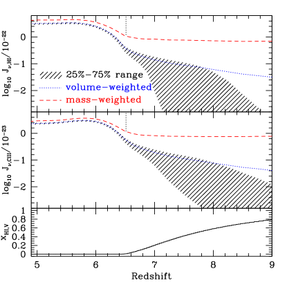
Figure 4: The scatter in the simulated radiation field at the HI (top) and $\mathrm{C\,III}$ (middle) ionization edges. For reference, we include the volume-averaged neutral fraction in the bottom panel and use vertical segments to indicate the reionization redshift as in Figure 1. The UVB amplitude varies by orders of magnitude prior to the completion of reionization. When considering only the galaxy contribution, the mass-weighted UVB is always stronger than the volume-weighted UVB, which suggests that the volume-averaged UVB underestimates the field that metal absorbers experience by $>30\%$ for $z>4$.

As observations push into the reionization epoch, the UVB becomes increasingly inhomogeneous. A key strength of our model is its ability to capture this inhomogeneity down to length scales of 30–40 proper kiloparsecs, which is roughly half the distance out to which metals travel ($\sim 100$ proper kpc; Oppenheimer & Davé 2008). Given that galaxies cluster on much larger scales, our simulation is therefore beginning to resolve the impact of the local field on metal absorbers. In order to assess whether this could play a role in our predictions, we show in Figure 4 the interquartile range as well as the volume-weighted and mass-weighted UVB ($J_{V}$ and $J_{M}$, respectively) at the $\mathrm{H\,I}$ and $\mathrm{C\,III}$ ionization edges as a function of redshift. To compute $J_{M}$, we weight the UVB in each radiation transport voxel by the amount of collapsed mass that it contains; this presumably provides a fair representation of the field near virialized regions. Note that Figure 4 does not include the calibration discussed in Section 3.1 as doing so would obviously leave results regarding spatial fluctuations unchanged.

Not surprisingly, the UVB fluctuates enormously prior to the epoch of overlap (we define this is the redshift where the volume-averaged neutral hydrogen fraction drops below 1%; this occurs at $z=6.5$ in our simulation). What is perhaps surprising is how quickly it becomes inhomogeneous: already if the neutral fraction is only 10% (which it may be at $z=7$; Bolton et al. 2011; Bolton & Haehnelt 2013), the interquartile range spans a factor of 2.5 (2) at the $\mathrm{H\,I}$ ($\mathrm{C\,III}$) ionization edges. The obvious implication is that it is inappropriate to model metal absorbers with a homogeneous UVB at redshifts where the neutral fraction is greater than $\sim 10\%$; the local field will dominate the photoionization rate.

Following reionization, fluctuations are at the $\sim 10\%$ level. Interestingly, $J_{M}>J_{V}$ at all times, and the difference is larger than the interquartile range. Even at $z=5$, when the mean free path to ionizing photons is much larger than our simulation volume (Worseck et al., 2014), $J_{M}/J_{V}$ is 1.3 (1.2) at the $\mathrm{H\,I}$ ($\mathrm{C\,III}$) ionization edges. This means that, as long as the UVB is not dominated by AGN, it is not possible for models to predict the abundance of metal absorbers to better than this accuracy unless they take local-field effects into account. Importantly, this is true even for optically-thin ions that are seen out to large impact parameters (such as $\mathrm{C\,IV}$). This is in contrast to the Lyman-$\alpha$ forest, which is relatively insensitive to the large spatial fluctuations that exist at $z>5$ because it is dominated by gas that lives in overall less biased regions (Mesinger & Furlanetto, 2009).

4 Comparison With a Volume-Averaged UVB

The most important differences between our current simulation and previous work are (1) The introduction of a spatially-resolved UVB; and (2) A subgrid treatment for self-shielding that explicitly attenuates the UVB in dense regions. In this section, we compare where absorbers lie in temperature-density space within our model versus expectations from the HM12 background in order to indicate what physical conditions $\mathrm{C\,II}$ and $\mathrm{C\,IV}$ absorbers trace in each case. We then show how the overall ionization state of carbon evolves in order to motivate a discussion of the evolving abundance of $\mathrm{C\,II}$ and $\mathrm{C\,IV}$ absorbers.

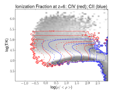
Figure 5: Solid red and blue contours indicate the mass fraction of carbon that is in $\mathrm{C\,IV}$ and $\mathrm{C\,II}$ as a function of density and temperature at $z=6$ using our simulated UVB with the normalization discussed in Section 3. Dashed contours are the same, but adopting the spatially-uniform HM12 UVB. Gray shading is proportional to the logarithm of the mean carbon mass fraction. Broadly, the simulated UVB yields significantly more ionized gas even though the two backgrounds are calibrated to match at the hydrogen ionization edge.

We show in Figure 5 how the mass fractions of carbon in $\mathrm{C\,II}$ and $\mathrm{C\,IV}$ (blue$=f_{\mathrm{C\,II}}$ and red$=f_{\mathrm{C\,IV}}$, respectively) vary with temperature and density at $z=6$ in the presence of our (spatially-inhomogeneous) renormalized UVB (solid) as compared to the spatially-uniform HM12 UVB (dashed). Broadly, the behaviour is similar to the results presented in ODF09: $\mathrm{C\,IV}$ prefers gas whose density is at or below the mean and has temperatures below $10^{5}$K, indicating an origin in photoionization. Meanwhile, $\mathrm{C\,II}$ prefers gas with densities more than $30\times$ the cosmic mean and temperatures below 50,000 K.

Comparing the dashed and solid curves, we see that our simulated UVB pushes the contours to higher density with respect to the HM12 model. In other words, gas is more highly ionized at all densities less than $\sim 100$. The generally higher ionization state reflects the impact of the local radiation field. At higher densities, self-shielding boosts the model’s $\mathrm{C\,II}$ fraction with respect to expectations from the HM12 UVB.

These differences have implications for the relationship between galaxies and absorbers. ODF09 find that, during the reionization epoch, $\mathrm{C\,IV}$ traces the locations of relatively massive galaxies because only they can expel metals out to the low densities where $\mathrm{C\,IV}$ becomes the dominant ionization state. Meanwhile, $\mathrm{C\,II}$ prefers higher densities and hence dominates in regions that are closer to the originating galaxies, and since low-mass galaxies dominate by number, they host most of the $\mathrm{C\,II}$ absorbers. Given that the local UVB boosts the ionization parameter near halos, it increases the $\mathrm{C\,IV}$ mass fraction and suppresses $\mathrm{C\,II}$ at all masses.

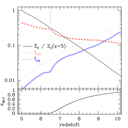
Figure 6: The evolution of the IGM’s carbon metal mass fraction $Z_{c}$ (normalized to its value at $z=5$) and the volume-weighted mass fractions that are in $\mathrm{C\,IV}$ and $\mathrm{C\,II}$. The bottom panel shows the simulated reionization history while the vertical segment in the top panel indicates the simulated reionization redshift. Heavy and light curves show results from our simulated UVB and the HM12 UVB, respectively. From $z=5$–10, both $Z_{C}$ and $f_{\mathrm{C\,IV}}$ increase while $f_{\mathrm{C\,II}}$ decreases. Meanwhile, the simulation predicts generally more ionized gas than the HM12 UVB owing to the local field from galaxies. This figure clearly shows that observations need to transition to low-ionization ions as they approach the reionization epoch.

In Figure 6, we elaborate on this point and move a step closer to observational implications by showing how the volume-weighted mass fractions of carbon in $\mathrm{C\,II}$ and $\mathrm{C\,IV}$ evolve along with the IGM carbon metal mass fraction $Z_{C}$, normalized to its value at $z=5$. Here, we define as “IGM” any gas that is not star-forming. Note that the normalizations of these curves are different from those of the total ion abundances $\Omega_{\mathrm{C\,II}}$ and $\Omega_{\mathrm{C\,IV}}$ (which we will explore in Figure 10) because the latter are weighted to high cross sections and columns. Nonetheless, they give qualitative insight into the expected observational trends. For reference, we include the volume-averaged neutral hydrogen fraction in the bottom panel.

Focusing on the heavy curves first, our simulation predicts that $f_{\mathrm{C\,II}}$ declines from 20–30% at $z=10$ to $<1\%$ by $z=5$. Over the same interval, $f_{\mathrm{C\,IV}}$ grows from 10% to 50%. In other words, $f_{\mathrm{C\,II}}$ and $f_{\mathrm{C\,IV}}$ essentially “swap places” during this epoch. It follows that observations should transition from high-ionization to low-ionization absorbers as they approach the reionization epoch, as that is where most of the carbon is. We will discuss how the abundance of $\mathrm{C\,II}$ and $\mathrm{C\,IV}$ absorbers is predicted to evolve at $z>5$ in Section 6.

The thin dashed and dotted curves show what is expected if we replace our renormalized UVB with the HM12 model. Despite the fact the two backgrounds match at the hydrogen ionization edge, the simulated UVB predicts significantly more $\mathrm{C\,IV}$ and less $\mathrm{C\,II}$. This reflects the fact that the UVB experienced by metals is stronger than the volume-averaged field. It is interesting to note that self-shielding does not cancel the impact of the the local field on $\mathrm{C\,II}$. This is because it boosts the $\mathrm{C\,II}$ mass fraction predominantly in highly overdense regions (Figure 5) whereas Figure 6 is weighted toward lower densities.

The behavior in Figure 6 is in qualitative agreement with the observation by Becker et al. (2011) that their observed sample of low-ionization systems was skewed to the higher-redshift portion of their survey. In the next section, we map Figure 6 into observable spaces and ask how its predictions could be tested.

5 Comparison with Observations

In this section, we study the predicted abundance of $\mathrm{C\,II}$ and $\mathrm{C\,IV}$ absorbers. We will show that our simulation reproduces the observed abundance of $\mathrm{C\,IV}$ and $\mathrm{C\,II}$ absorbers at $z=6$ in the regime where the simulated and observed dynamic ranges overlap, and at $z=3$ for $\mathrm{C\,IV}$ absorbers with $\log(N_{\mathrm{C\,IV}})>14$.

5.1 Generating Simulated Spectra

We begin by discussing how we extract simulated spectra from our model and compute the abundance of absorbers. At each redshift, we cast a sightline that is oblique to the simulation boundaries and wraps around it until subtending a Hubble velocity width of $5\times 10^{5}\;{\rm km}\,{\rm s}^{-1}$. This corresponds to an absorption path length (e.g., Equation 2 of Becker et al., 2011) of 20–100, depending on the redshift. The line of sight is divided into bins whose width $\Delta$ in configuration space corresponds to a separation of $2\;{\rm km}\,{\rm s}^{-1}$ in a pure Hubble flow; that is, $\Delta\times H(z)=2\;{\rm km}\,{\rm s}^{-1}$. We smooth particles that overlap the line of sight to the radiation field’s grid in order to compute the local ionization rates of all ions of O, C, and Si. Next, we compute the equilibrium ionization state of these atoms using the local temperature, density, metallicity, and UVB (where we emply the renormalized UVB unless stated otherwise). Our ionization solver accounts for photoionization, collisional ionization, direct and dielectronic recombination, and charge transfer recombination. Photoionization cross-sections are taken from Verner et al. (1996); collisional photoionization rates are from Voronov (1997); direct and dielectronic recombinations are from Badnell (2006) and Badnell et al. (2003), respectively; and charge transfer recombination rates are from Kingdon & Ferland (1996). The local hydrogen ionization state is fixed to the nonequilibrium value stored in the simulation snapshot, and the electron abundance is taken as the value from the simulation owing to ionization of hydrogen and helium plus the small contribution from ionized metals. This approach is essentially equivalent to running CLOUDY (Ferland et al., 1998) on each gas particle because we use the same cross-sections and rates except that we neglect Auger ionization.

We derive each transition’s optical depth along the sightline as a function of velocity following a standard approach that takes thermal and bulk motions into account (for example, Theuns et al., 1998). We then smooth the predicted transmission with a Gaussian kernel whose full-width at half maximum is $10\;{\rm km}\,{\rm s}^{-1}$ in the rest-frame and add random noise corresponding to a signal-to-noise of 50 per pixel. Finally, we use autovp (Davé et al., 1997) with the default parameters to identify absorption systems and compute column densities.

In order to make a fair comparison to observations, we follow standard practice and merge all absorbers that lie within $50\;{\rm km}\,{\rm s}^{-1}$ of each other into “systems” and add their column densities. In what follows, we will will use the terms “systems”, “absorbers,” and “absorption systems” interchangeably.

5.2 Column Density Distribution

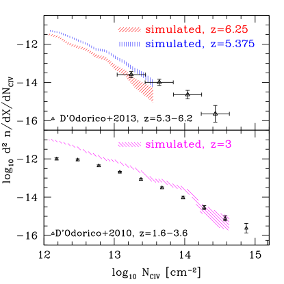
Figure 7: Simulated column density distribution versus observations at $z\approx 5$–6 (top panel) and $z=1.6$–3.6 (bottom panel). The simulated range reflects sqrt(N) uncertainty. We have multiplied the D’Odorico et al. (2013) measurements by 1.07 and the D’Odorico et al. (2010) measurements by 1.197 to adjust to our cosmology. The predicted abundance near the end of the reionization epoch shows good agreement with observations in the column density range $\log(N_{\mathrm{C\,IV}})=$13–13.5, with an abundant population of absorbers predicted at lower columns. By $z=3$, the simulation overpredicts the observations, particularly at the low-column end.

In the top panel of Figure 7, we compare the simulated column density distribution (CDD) of $\mathrm{C\,IV}$ absorption systems at $z\sim 6$ versus the observations of D’Odorico et al. (2013) at $z=5.3$–6.2, where we have adjusted their measurements to match our assumed cosmology. We find reasonable agreement in the range $\log(N_{\mathrm{C\,IV}})=$13–13.5. This suggests that the assumed carbon yields and outflow scalings at the reionization epoch are broadly realistic. Unfortunately, the simulation underproduces systems with larger columns. This reflects a well-known numerical artefact whereby small simulation volumes whose mean matter density equals the cosmic value systematically lack the massive systems that dominate $\mathrm{C\,IV}$ absorbers at high redshift.

Our high mass resolution allows us to predict the CDD down to lower columns than previous works (such as Cen & Chisari, 2011); this is the tradeoff for our much smaller simulation volume. We find that the predicted CDD remains quite steep down to at least $10^{12}$ cm^-2, as directly observed at lower redshifts (bottom panel). Future observations probing to lower columns will therefore impose stronger constraints both on our newest outflow model and, more generally, on reionization models in which galaxies in photosensitive halos dominate the ionizing background.

In the bottom panel, we compare the predicted column density distribution at $z=3$ versus the D’Odorico et al. (2010) observations at $z=1.6$–3.6. At high columns ($\log(N_{\mathrm{C\,IV}})>14$), the predicted CDD lies within $1\sigma$ of observations. At lower columns, the model overpredicts observations by 2–3$\times$, which is much larger than the measurement uncertainty. Note that observational completeness is not expected to be the main problem: D’Odorico et al. (2010) estimate a completeness of 60% at $10^{12}$cm^-2 and $>90\%$ for $\log(N_{\mathrm{C\,IV}})>12.6$.

If the discrepancy owes to the simulated UVB, then it must owe either to its slope or to spatial fluctuations rather than the amplitude, which is reasonably well-constrained at $z=3$ (recall that we calibrate it to match the HM12 model at the $\mathrm{H\,I}$ ionization edge). Obviously, the tendency for the UVB to be stronger near galaxies contributes, but only at the 30% level (Section 3.3). Moreover, we believe this is a real effect, so it cannot be the true problem. An alternative explanation is that our model underestimates the UVB at the $\mathrm{C\,IV}$ ionization edge owing to delayed HeII reionization (Section 3.2); in other words, the model underestimates the mass fraction that is photoionized to $\mathrm{C\,V}$ and higher ionization states because the opacity bluewards of 4 Ryd is too strong.

It is also possible that the model overproduces $\mathrm{C\,IV}$ because it ejects too many metals into the IGM. We disfavor this interpretation because, as we will show in Figure 8, our model reproduces the observed abundance of $\mathrm{C\,II}$ absorbers. Suppressing outflows in order to reduce the number of $\mathrm{C\,IV}$ absorbers would cause the model to underproduce $\mathrm{C\,II}$ severely.

Finally, we note that, if numerical limitations are any problem at all at $z=6$, then they are a much bigger one at $z=3$ because small simulation volumes miss a progressively larger fraction of collapsed structure at lower redshifts (Barkana & Loeb, 2004). At a glance, it is therefore quite surprising that our simulation extends to higher columns at $z=3$ than at $z=6$. The explanation may be found in the tendency for $\mathrm{C\,IV}$ to trace higher overdensities at lower redshifts (ODF09; D’Odorico et al., 2013). The higher the characteristic overdensity of an ion, the more rapidly galaxies can enrich their surroundings to the point where that ion becomes observable. Consequently, limitations associated with our small simulation volume are less severe for $\mathrm{C\,IV}$ at lower redshifts, particularly when considering absorbers in a fixed range in column density.

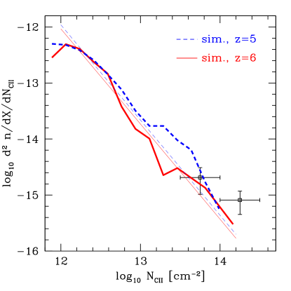
Figure 8: Simulated $\mathrm{C\,II}$ CDD at two different redshifts as indicated. Data are derived from 9 observed $\mathrm{C\,II}$ systems at absorption redshifts of 5.57–6.25 (see text), with vertical errors indicating sqrt(N). Thin curves indicate best-fit power laws assuming a constant slope of -1.7. The simulation reproduces observations within the errors, indicating that the simulated CGM and radiation fields are broadly realistic.

In Figure 8, we compare the predicted $\mathrm{C\,II}$ CDD to observations.  Becker et al. (2011) identified 7 $\mathrm{C\,II}$ systems in high-resolution spectra of 9 quasars that have a mean emission redshift of 6; 6 of these have column densities above $10^{13.5}$cm^-2, where they report more than 50% completeness.  D’Odorico et al. (2013) identified 5 $\mathrm{C\,II}$ systems in lower-resolution spectra of 6 quasars whose mean emission redshift is 5.7. Three of these quasars and two of the $\mathrm{C\,II}$ systems were also observed at higher resolution by Becker et al. (2011). We combine these samples, adopting the Becker et al. (2011) column densities for the two absorbers in the spectrum of SDSS J0818+1722. This yields a total of 9 $\mathrm{C\,II}$ systems with column densities above $10^{13.5}$cm^-2. We assume that each sightline surveys an absorption path length of 2.37, for a total surveyed path length of 28.44. Our simulation reproduces the observed $\mathrm{C\,II}$ CDD within the errors.

In summary, the level of agreement between the predicted and observed $\mathrm{C\,II}$ and $\mathrm{C\,IV}$ CDDs in Figures 7–8 suggests that the metallicity, temperature, and radiation field of the reionization-epoch CGM in our model are realistic. The fact that we have not tuned any parameters in order to match these observations supports the view that current observations of metal absorbers do not require additional physical inputs such as metals or light from Population III stars (see also Kulkarni et al., 2013) or a strong contribution from X-ray binaries to the UVB (Jeon et al., 2014).

6 Predictions

6.1 Integrated Abundances

In this section, we predict the integrated abundance of $\mathrm{C\,II}$ and $\mathrm{C\,IV}$ absorbers as a function of redshift. In order to correct for the limitations that we identified in Figures 7 and 8, we extrapolate from our simulation as follows: First, we assume that the simulated $\mathrm{C\,IV}$ and $\mathrm{C\,II}$ CDDs are complete over the column density range $10^{12}$–$10^{13}$cm^-2. Next, we assume that they follow power-laws with slopes of -1.7 (where the slope for $\mathrm{C\,II}$ is inferred from Figure 8 and the slope for $\mathrm{C\,IV}$ is supported by D’Odorico et al. 2013), and use the predicted abundances of systems with columns in the resolved range to normalize. Finally, we compute the predicted number of systems with column densities in the range $10^{13}$–$10^{15}$cm^-2 per absorption path length as a function of redshift. For reference, we also include the expected number of systems in the expanded range $10^{12}$–$10^{15}$cm^-2 as the lower-column systems will be observable using the next generation of thirty-meter telescopes.

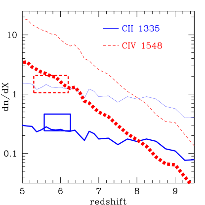
Figure 9: The predicted number of $\mathrm{C\,II}$ (solid blue) and $\mathrm{C\,IV}$ (dashed red) systems per unit absorption path length as a function of redshift. Heavy curves indicate the expected number of systems in the column density range $10^{13}$–$10^{15}$cm^-2, whereas thin curves correspond to a next-generation survey encompassing $10^{12}$–$10^{15}$cm^-2. All curves include an extrapolation as described in the text. The predicted number of $\mathrm{C\,II}$ systems evolves slowly while the predicted $\mathrm{C\,IV}$ abundance decreases strongly with increasing redshift. The solid blue and dashed red boxes indicate $\mathrm{C\,II}$ and $\mathrm{C\,IV}$ observations, respectively.

In Figure 9, we show how the total number of systems per path length is predicted to evolve with redshift. Perhaps the most important takeaway from this figure is what is not seen, namely a sharp feature in the abundance of $\mathrm{C\,II}$ and $\mathrm{C\,IV}$ systems at the reionization redshift ($z=6.5$). This reflects the fact that carbon is ionized by local sources long before reionization is complete. Going to lower column densities does not help because lower column densities are populated by systems with lower masses, which are quite abundant. Hence our model indicates that metal absorbers are sensitive both to ongoing enrichment and to reionization. We will return to this point in Figure 13.

The abundances of $\mathrm{C\,II}$ and $\mathrm{C\,IV}$ systems evolve in very different ways. In particular, the abundance of $\mathrm{C\,II}$ systems evolves very slowly owing to a tradeoff between the competing effects of enrichment and ionization (as was also noted in ODF09 and Finlator et al., 2013). Meanwhile, the abundance of $\mathrm{C\,IV}$ systems increases strongly with decreasing redshift because the strengthening ionizing background, increasing metallicity, and decreasing overall gas densities all push an increasing fraction of the IGM into the range favoring $\mathrm{C\,IV}$.

For a constant minimum column density, the abundance of $\mathrm{C\,IV}$ systems eventually drops below the $\mathrm{C\,II}$ abundance. This is qualitatively consistent with the observation that $\mathrm{C\,IV}$ is not observed past $z=6$ (Becker et al., 2011), although Figure 9 predicts that $\mathrm{C\,IV}$ absorbers vanish much more slowly.

The solid blue box indicates the observed $\mathrm{C\,II}$ abundance. We compute this by taking the 10 $\mathrm{C\,II}$ systems from 12 sightlines observed by Becker et al. (2011) and D’Odorico et al. (2013), each of which is assumed to probe a path length of 2.37. The vertical error is sqrt(N). This estimate is in marginal agreement with the prediction. Correcting the data for the known incompleteness over this column density range ($>50\%$ for $N_{\mathrm{C\,II}}<10^{13.5}$cm^-2; Becker et al. 2011) would boost the observed abundance and degrade the level of agreement. On the other hand, increasing our simulation volume would likewise boost the predicted abundance by sampling the mass function more completely (Barkana & Loeb, 2004). Given these uncertainties, we conclude that the predicted $\mathrm{C\,II}$ abundance is consistent with current observations.

The dashed red box indicates the observed abundance of $\mathrm{C\,IV}$ absorbers from $z=5.3$–6.2. We compute the observed value by using a least-squares approach to fit power-laws to the measurements of D’Odorico et al. (2013) and extrapolating to encompass the range $10^{13}$–$10^{15}$cm^-2. Although current observations do not constrain the power-law parameters tightly (D’Odorico et al., 2013), this extrapolation is fairly robust because it only strays slightly outside the observed range. The resulting best-fit value and 67% confidence interval is $1.3^{+0.8}_{-0.2}$ for a fiducial slope of -1.7. This is in good agreement with the simulation, particularly at $z\sim 6$.

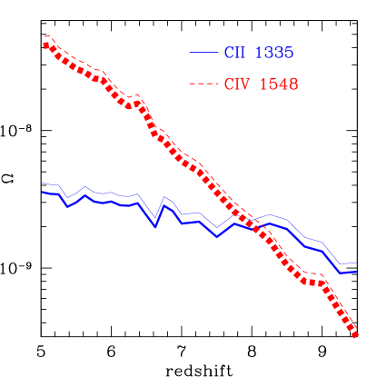
Figure 10: The predicted mass density in $\mathrm{C\,II}$ (solid blue) and $\mathrm{C\,IV}$ (dashed red) systems as a function of redshift. Heavy curves sum over systems in the column density range $10^{13}$–$10^{15}$cm^-2, whereas thin curves correspond to a next-generation survey encompassing $10^{12}$–$10^{15}$cm^-2.

We next show in Figure 10 how the predicted mass density in each ion relative to the critical mass density evolves with redshift using the same column density ranges as in Figure 9. Broadly, the same trends are seen as before: $\Omega_{\mathrm{C\,IV}}$ evolves rapidly whereas $\Omega_{\mathrm{C\,II}}$ evolves slowly, with the two crossing at $z=8$. This may be slightly too early: As noted in Section 1, observations indicate that $\Omega_{\mathrm{C\,II}}>\Omega_{\mathrm{C\,IV}}$ at $z=6$. We attribute this discrepancy to uncertainty in the CDD slopes, which are poorly-constrained at these redshifts. Our assumption that both CDDs have power-law slopes of -1.7 affects Figure 10 more strongly than Figure 9 because it weights the $\Omega$s toward the strongest absorbers, where the model is most incomplete. If, for example, the $\mathrm{C\,II}$ slope were flatter or the $\mathrm{C\,IV}$ slope steeper, then they would cross at a later redshift.

In summary, our model reproduces the observed number of $\mathrm{C\,IV}$ and $\mathrm{C\,II}$ absorbers per path length at $z\sim 6$ within the uncertainties, and assuming that both CDDs have slopes of -1.7 leads to the prediction that $\Omega_{\mathrm{C\,IV}}$ and $\Omega_{\mathrm{C\,II}}$ cross at $z\approx 8$. The former prediction is constrained and reasonably robust, while the latter will need to be revisited using calculations that treat a larger dynamic range in order to model the CDDs’ power-law slopes more precisely.

6.2 Scatter

Up until now we have considered the total number of absorption systems, but we have not investigated the scatter in the number per line of sight. This could be significant for $\mathrm{C\,II}$ systems because there is roughly 1 per line of sight at $z=6$. For example, Becker et al. (2011) identify 7 systems along 9 sightlines. Four of their systems lie along a single sightline while 6 sightlines have no low-ionization absorption at all (although one of these 6, SDSS J1030+0524, does yield up a $\mathrm{C\,II}$ absorber in the X-shooter spectrum of D’Odorico et al. 2013). Combining the Becker et al. (2011) and D’Odorico et al. (2013) samples, all of the observed $\mathrm{C\,II}$ systems are accounted for by only one third of their sightlines. Does this indicate that the Universe is partially neutral at $z=6$ or could it reflect ordinary galaxy clustering? These considerations motivate an inquiry into the scatter in the number of systems per observed line of sight or per survey. Our simulated sightlines subtend absorption path-lenghths of 20–100, while a single observed line of sight at $z\sim 6$ can only probe $\mathrm{C\,II}$ systems over a path length of 2–3, hence we may use our simulation to study the scatter in the predicted number of absorbers. In practice, this will underestimate the actual scatter owing to our small simulation volume, but it is nonetheless a useful first step.

We begin by breaking up our simulated lines of sight into individual segments whose absorption path length corresponds to the redshift distance over which $\mathrm{C\,II}$ is observable in a quasar at that redshift. This is taken to be the distance between Lyman-$\alpha$ in the quasar rest-frame and 5000 $\;{\rm km}\,{\rm s}^{-1}$ bluewards of the $\mathrm{C\,II}$ 1334 transition (mimicking observational efforts to avoid the quasar’s proximity zone). Note that, throughout this section, we use the simulated number of absorbers “out of the box” rather than correcting for missing strong absorbers as in Figures 9–10. This will lead us to underestimate the predicted number of systems with columns greater than $10^{14}$cm^-2, but not have much effect at lower columns.

Figure 11: The distribution in the predicted number of $\mathrm{C\,II}$ systems with column density greater than $10^{13}$cm^-2 per sightline at two redshifts and in observations. All histograms are normalized to unit area. Both the simulation and the observations find many sightlines with no systems at all and a small number of sightlines with one or more.

In Figure 11, we show the distribution in the predicted number of systems per sightline at two representative redshifts and in the observations. For reference, the observations consist of 12 independent sightlines while the simulation yields 23 at each redshift. Broadly, the simulation reproduces both the tendency for a large number of sightlines to contain no systems at all and an occasional sightline to contain more than one. At the abundant end, three of 23 simulated sightlines drawn from the $z=5.75$ snapshot contain $\geq 3$ systems (and none at $z=6.25$). By comparison, one of 12 observed sightlines contains 4 systems at $z=$6.13–6.25. At the same time, more than half of sightlines have no absorbers both in the models and the data. We conclude that, subject to our numerical limitations and the small current sample sizes, our simulation reproduces the observed clustering behavior of $\mathrm{C\,II}$ systems. Given that our simulation volume completes reionization at $z=6.5$, this implies that $\mathrm{C\,II}$ observations are consistent with a completely reionized Universe.

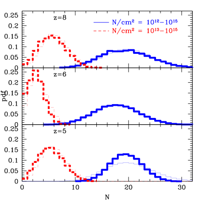
Figure 12: The distribution in the predicted number of $\mathrm{C\,II}$ systems observed in hypothetical surveys covering 6 quasars (or GRBs) at three different redshifts and two different column density ranges. Heavy and thin curves indicate the raw simulated number of systems and Poisson distributions with the same means. The predicted number of systems is skewed to low numbers with respect to a matching Poisson distribution.

Having studied the scatter in the number of absorbers per sightline, we assemble 10,000 mock “surveys” by drawing 6 simulated sightlines at random and compiling the number of absorbers in two ranges of column density. In Figure 12, we use heavy curves to show the distribution in the total number of systems per survey at three redshifts and in two column density ranges. The mean number of systems per mock survey increases from $z=5$ to $z=8$ because the increasing path length per sightline more than cancels the declining intrinsic number of systems per path length (Figure 9). In fact, these effects give rise to a local minimum in the predicted number of systems per path length which appears to occur somewhere between $z=8$ and $z=5$. The effect is not seen in Figure 9 because the latter extrapolates from the predicted number of systems with columns of $10^{12}$–$10^{13}$cm²; it is therefore apparent only in stronger systems. Future work will be necessary in order to determine to what extent it reflects cosmic variance limitations.

For each combination of redshift and column density, we additionally use a thin curve to show the Poisson distribution corresponding to the same mean number of systems. In most cases, there are slightly more surveys with low numbers of systems than predicted by the Poisson distribution. At $z=8$ this could in principle reflect the presence of sightlines that subtend neutral regions, but by $z=5$ it indicates the impact of voids on absorber statistics. That the distributions are not significantly more skewed to low numbers at $z=8$ than at $z=5$ indicates that voids play a bigger role in generating the skew than neutral regions because carbon is ionized locally even in regions that are neutral on large scales.

6.3 Evolution in Gas or UVB?

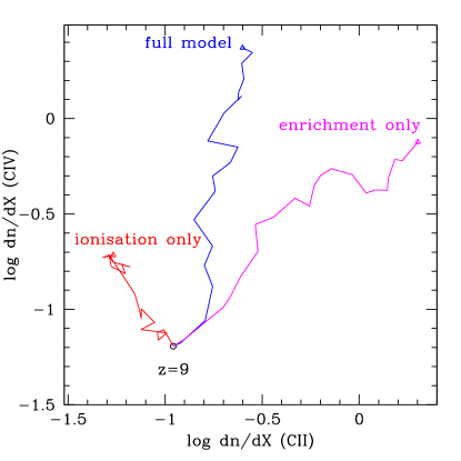
Figure 13: The predicted evolution in the number of absorption systems per path length from $z=9\rightarrow 5.5$ in our fiducial case (blue) versus a toy model in which no extra metals are ejected after $z=9$ (red) and a model where the UVB does not evolve after $z=9$ (magenta). Evolution in the UVB and the CGM both contribute to the overall evolution in absorber abundance.

A central question in interpreting metal absorbers regards what drives their evolution. The three major contributing factors are the growing UVB, the declining mean density of CGM gas, and ongoing enrichment. If evolution is primarily driven by a growing UVB, then (1) metal absorbers are a complementary tracer of reionization (Oh, 2002; Furlanetto & Loeb, 2003); and (2) the observed metals are the signature of a very early generation of stars. If evolution is primarily driven by a tradeoff between continuing enrichment and declining densities, then observations trace ongoing star formation in low-mass galaxies (Becker et al., 2011).

In order to address this question, we re-compute the predicted number of $\mathrm{C\,II}$ and $\mathrm{C\,IV}$ absorbers per path length in the column density range of $10^{13}$–$10^{15}$cm^-2 ($l_{\mathrm{C\,II}}$ and $l_{\mathrm{C\,IV}}$, respectively) in two toy-model scenarios. First, we take the gas density and metallicity from our $z=9$ snapshot while allowing the UVB to evolve down to $z=5.5$. This “ionization-only” scenario is illustrated by the red trajectory in Figure 13 leading upwards and to the left. Quite intuitively, a growing UVB suppresses $l_{\mathrm{C\,II}}$ and boosts $l_{\mathrm{C\,IV}}$. In the second toy-model, we allow the gas density and metallicity to evolve but leave the UVB fixed (in proper units) to the $z=9$ field. This “enrichment-only” model is indicated by the magenta trajectory leading to increasing $l_{\mathrm{C\,II}}$ and $l_{\mathrm{C\,IV}}$. In this case, there is fairly continuous growth in both $l_{\mathrm{C\,II}}$ and $l_{\mathrm{C\,IV}}$. The full model runs between these two. We conclude that the evolving population of carbon absorbers does not predominantly trace either UVB or CGM evolution because they either cancel (in the case of $l_{\mathrm{C\,II}}$) or both drive signicant evolution (in the case of $l_{\mathrm{C\,IV}}$). Instead, it is sensitive to both.

6.4 Large-Scale Fluctuations in the UVB

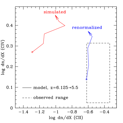
Figure 14: The impact of our renormalized field on the predicted number of systems per path length from $z=6\rightarrow 5.5$. Renormalizing the UVB to boost $\tau_{\mathrm{Ly}\alpha}$ suppresses $\mathrm{C\,IV}$ modestly while boosting the number of $\mathrm{C\,II}$ systems by $\approx 4\times$. The dashed box shows the observationally-allowed region from Figure 9.

The observable space in Figure 13 is a convenient setting for exploring how large-scale spatial fluctuations in the UVB might impact our predictions. In particular, Becker et al. (2014) have recently argued that the UVB may be inhomogeneous down to $z=5$ on scales that are not captured by our simulation. We showed in Figure 2 that the simulated and renormalized UVBs roughly span the observed range of $\tau_{\mathrm{Ly}\alpha}$ measurements from $z=5$–6. We now use this fact to bracket the uncertainty owing to large-scale UVB fluctuations. In Figure 14, we show how $l_{\mathrm{C\,II}}$ and $l_{\mathrm{C\,IV}}$ evolve from $z=6.125\rightarrow 5.5$ using the simulated (left) and renormalized (right) UVBs, while the dashed box indicates the same observations as in Figure 9. The simulated UVB overproduces $l_{\mathrm{C\,IV}}$ and underproduces $l_{\mathrm{C\,II}}$, indicating that its amplitude is on average too high. Renormalizing the UVB increases $l_{\mathrm{C\,II}}$ by a factor of 3–4 and reduces $l_{\mathrm{C\,IV}}$ abundance by 0.1 dex. To the extent that the simulated and renormalized UVBs span the realistic range, the converged value will lie somewhere between these curves. On the other hand, given that the renormalized field is not weak enough to match the regions where flux is undetected in Figure 2, the true correction may be somewhat larger still.

7 Summary

7.1 Summary of Results

We have used a cosmological hydrodynamic simulation that models a spatially-inhomogeneous multifrequency ionizing background on-the-fly to study how the abundance of $\mathrm{C\,II}$ and $\mathrm{C\,IV}$ absorbers evolves through the latter half of the hydrogen reionization epoch. Our results are as follows:

• The volume average of our simulated radiation field is within a factor of 2–4$\times$ of the spatially-uniform HM12 model down to $z=3$; this discrepancy is not large compared to observational uncertainties.

• Consistently with observations, the predicted UVB at the HI ionization edge does not evolve strongly between $z=$6–3.

• The mean radiation field shows large spatial fluctuations on scales that metal absorbers are sensitive to and is stronger than the volume-average in regions where metals lurk, indicating that models cannot predict the abundance of metal absorbers to better than 20–30% accuracy unless they account for local sources.

• Our model matches the observed $\mathrm{C\,IV}$ and $\mathrm{C\,II}$ abundances at $z=6$ and slightly overproduces low-column $\mathrm{C\,IV}$ absorbers at $z=3$. Meanwhile, it does not reproduce the observed mass densities at $z\sim 6$, indicating that further work is necessary to constrain the CDD slopes.

• The volume-averaged mass fraction, absorber abundance, and mass density of $\mathrm{C\,IV}$ decrease to high redshifts. Meanwhile, the $\mathrm{C\,II}$ mass fraction increases owing to weakening UVB and the increasing proper density of metal-bearing regions. However, the overall $\mathrm{C\,II}$ absorber abundance and ion mass density decrease slowly with increasing redshift because the CGM metallicity decreases.

• The abundances and mass densities of $\mathrm{C\,II}$ and $\mathrm{C\,IV}$ are predicted to cross at $z=8$, reflecting evolution in the volume-averaged mass fractions.

• The predicted number of low-ionization absorbers per quasar sightline shows roughly the same scatter as observations, with the implication that the observed scatter does not require a partially-neutral universe at $z=6$. There are somewhat more sightlines with zero absorbers than predicted by Poisson statistics, indicating the influence of voids.

7.2 Summary of Limitations

The major drawback of our simulation is its small volume, which introduces three limitations. First, we saw in Section 3 that our simulation predicts an artificially rapid rise in the UVB amplitude at the overlap epoch. We compensate for this by normalizing the simulated UVB so that its volume average does not exceed the HM12 model at the $\mathrm{H\,I}$ ionization edge. In practice, this means scaling the entire simulated UVB at each redshift below $z=6.5$ by a factor that ranges from 2 to 4. This calibration preserves the simulated UVB’s spectral slope and spatial fluctuations while preventing the artefact from propagating into our predictions.

Unfortunately, Figure 2 shows that this calibration does not bring the predicted Lyman-$\alpha$ optical depth into complete agreement with observations owing to the second problem, which is an inaccurate sampling of voids and overdensities. Lyman-$\alpha$ transmission occurs in voids where the neutral fraction is lower (Bolton & Becker, 2009), hence it requires large volumes. Meanwhile, metal absorbers occur in overdensities where galaxies form, hence they require high resolution in order to capture the dominant, low-mass galaxy population.

The final consequence of our small volume is the incomplete overlap between the simulated and observed column density ranges at $z=6$. This occurs because our simulation systematically lacks the massive halos that host high-column systems (Figures 8–7). We compensate for this by extrapolating the predicted CDDs assuming power-law slopes of -1.7.

In short, increasing our dynamic range will simultaneously yield a smoother reionization history, a more realistic representation of voids and overdensities, and a more accurate model for the CDD. These improvements will enhance our ability to understand how metal absorbers probe the galaxies, enriched CGM, and UVB that had formed by the close of the reionization epoch.

Appendix

A Test of self-shielding

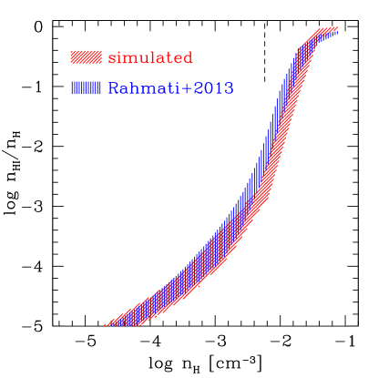
Figure 15: The 15–85% neutral hydrogen fraction range versus proper hydrogen number density at $z=3$ in our simulation (red, diagonal shading) and using the Rahmati et al. (2013) attenuation function (blue, vertical shading). The vertical dashed segment indicates a representative self-shielding threshold density of 0.006 cm^-3 (assuming a temperature of $10^{4}K$). The two ranges overlap at all densities, indicating that our self-shielding treatment attenuates the radiation field realistically.

As a test of our self-shielding prescription, we compare the simulated trend of neutral hydrogen fraction versus proper hydrogen number density $n_{H}$ at $z=3$ with the spatially-resolved study by Rahmati et al. (2013). We implement the Rahmati et al. (2013) attenuation model as follows: First, we compute the volume-averaged mean hydrogen photoionization rate directly from our simulation (their Equation 3). Next, we use their Equation 13 to compute the threshold density for self-shielding, adopting each particle’s local temperature in turn. Next, we use their Equation 14 to compute the attenuation. Finally, we use the attenuated photoionization rate to compute the equilibrium ionization fraction following Katz et al. (1996). Note that we do not employ the renormalised radiation field for this purpose (Section 3), hence the comparison is a direct test of the simulation.

Figure 15 shows that the two models are in broad agreement, indicating that our self-shielding model is realistic. In detail, however, the simulated neutral fraction is up to $3\times$ lower for densities $-2.5<\log(n_{H})<-1.5$, while for higher densities it is somewhat higher. We have directly verified that these slight differences do not reflect the helium ionization state, the predicted flux above 4 Ryd, or departures from ionization equilibrium. Instead, they suggest (1) that the simulated radiation field is insufficiently attenuated at densities near the self-shielding threshold; and (2) that very dense gas ($-1.5<\log(n_{H})$) is slightly too neutral in the simulation because we omit ionizing recombination radiation (see, for example, Figure 4 of Rahmati et al. 2013). The lack of recombination radiation is not a problem for our study because it is sharply peaked at 1 Ryd whereas the $\mathrm{C\,II}$ photoionization threshold is 1.8 Ryd. Hence while there is room for progress in accounting for small-scale radiative transfer effects accurately, we conclude that our simulation is adequate for our present purposes.

References

- Alvarez et al. (2012) Alvarez, M. A., Finlator, K., & Trenti, M. 2012, ApJL, 759, L38
- Badnell et al. (2003) Badnell, N. R., O’Mullane, M. G., Summers, H. P., et al. 2003, A&A, 406, 1151
- Badnell (2006) Badnell, N. R. 2006, ApJS, 167, 334
- Barkana & Loeb (2004) Barkana, R., & Loeb, A. 2004, ApJ, 609, 474
- Becker et al. (2009) Becker, G. D., Rauch, M., & Sargent, W. L. W. 2009, ApJ, 698, 1010
- Becker et al. (2011) Becker, G. D., Sargent, W. L. W., Rauch, M., & Calverley, A. P. 2011, ApJ, 735, 93
- Becker & Bolton (2013) Becker, G. D., & Bolton, J. S. 2013, MNRAS, 436, 1023
- Becker et al. (2014) Becker, G. D., Bolton, J. S., Madau, P., et al. 2014, arXiv:1407.4850
- Bolton & Becker (2009) Bolton, J. S., & Becker, G. D. 2009, MNRAS, 398, L26
- Bolton et al. (2011) Bolton, J. S., Haehnelt, M. G., Warren, S. J., et al. 2011, MNRAS, 416, L70
- Bolton & Haehnelt (2013) Bolton, J. S., & Haehnelt, M. G. 2013, MNRAS, 429, 1695
- Cen et al. (2005) Cen, R., Nagamine, K., & Ostriker, J. P. 2005, ApJ, 635, 86
- Cen & Chisari (2011) Cen, R., & Chisari, N. E. 2011, ApJ, 731, 11
- Cooksey et al. (2013) Cooksey, K. L., Kao, M. M., Simcoe, R. A., O’Meara, J. M., & Prochaska, J. X. 2013, ApJ, 763, 37
- Davé et al. (1997) Davé, R., Hernquist, L., Weinberg, D. H., & Katz, N. 1997, ApJ, 477, 21
- Davé et al. (2013) Davé, R., Katz, N., Oppenheimer, B. D., Kollmeier, J. A., & Weinberg, D. H. 2013, MNRAS, 434, 2645
- Díaz et al. (2014) Díaz, C. G., Koyama, Y., Ryan-Weber, E. V., et al. 2014, MNRAS, 442, 946
- D’Odorico et al. (2010) D’Odorico, V., Calura, F., Cristiani, S., & Viel, M. 2010, MNRAS, 401, 2715
- D’Odorico et al. (2013) D’Odorico, V., Cupani, G., Cristiani, S., et al. 2013, MNRAS, 435, 1198
- Duffy et al. (2014) Duffy, A. R., Wyithe, J. S. B., Mutch, S. J., & Poole, G. B. 2014, MNRAS, 443, 3435
- Eisenstein & Hu (1999) Eisenstein, D. J., & Hu, W. 1999, ApJ, 511, 5
- Fan et al. (2006) Fan, X., Strauss, M. A., Becker, R. H., et al. 2006, AJ, 132, 117
- Ferland et al. (1998) Ferland, G. J., Korista, K. T., Verner, D. A., et al. 1998, PASP, 110, 761
- Ferrara & Loeb (2013) Ferrara, A., & Loeb, A. 2013, MNRAS, 431, 2826
- Finlator et al. (2011) Finlator, K., Davé, R., Özel, F. 2011, ApJ, 743, 169
- Finlator et al. (2013) Finlator, K., Muñoz, J. A., Oppenheimer, B. D., et al. 2013, MNRAS, 436, 1818
- Furlanetto & Loeb (2003) Furlanetto, S. R., & Loeb, A. 2003, ApJ, 588, 18
- Furlanetto et al. (2004a) Furlanetto, S. R., Zaldarriaga, M., & Hernquist, L. 2004, ApJ, 613, 1
- Furlanetto et al. (2004b) Furlanetto, S. R., Zaldarriaga, M., & Hernquist, L. 2004, ApJ, 613, 16
- Furlanetto & Oh (2005) Furlanetto, S. R., & Oh, S. P. 2005, MNRAS, 363, 1031
- Haardt & Madau (2001) Haardt, F. & Madau, P. 2001, in proc. XXXVIth Rencontres de Moriond, eds. D.M. Neumann & J.T.T. Van.
- Haardt & Madau (2012) Haardt, F., & Madau, P. 2012, ApJ, 746, 125
- Hinshaw et al. (2013) Hinshaw, G., Larson, D., Komatsu, E., et al. 2013, ApJS, 208, 19
- Hopkins (2013) Hopkins, P. F. 2013, MNRAS, 428, 2840
- Iliev et al. (2014) Iliev, I. T., Mellema, G., Ahn, K., et al. 2014, MNRAS, 439, 725
- Jaacks et al. (2012) Jaacks, J., Choi, J.-H., Nagamine, K., Thompson, R., & Varghese, S. 2012, MNRAS, 420, 1606
- Jeon et al. (2014) Jeon, M., Pawlik, A. H., Bromm, V., & Milosavljević, M. 2014, MNRAS, 440, 3778
- Katz et al. (1996) Katz, N., Weinberg, D. H., & Hernquist, L. 1996, ApJS, 105, 19
- Kingdon & Ferland (1996) Kingdon, J. B., & Ferland, G. J. 1996, ApJS, 106, 205
- Kuhlen & Faucher-Giguère (2012) Kuhlen, M., & Faucher-Giguère, C.-A. 2012, MNRAS, 423, 862
- Kulkarni et al. (2013) Kulkarni, G., Rollinde, E., Hennawi, J. F., & Vangioni, E. 2013, ApJ, 772, 93
- Leitherer et al. (1999) Leitherer, C., Schaerer, D., Goldader, J. D., et al. 1999, ApJS, 123, 3
- Lidman et al. (2012) Lidman, C., Hayes, M., Jones, D. H., et al. 2012, MNRAS, 420, 1946
- Malloy & Lidz (2014) Malloy, M., & Lidz, A. 2014, arXiv:1410.0020
- McQuinn et al. (2011) McQuinn, M., Oh, S. P., & Faucher-Giguère, C.-A. 2011, ApJ, 743, 82
- Mesinger & Furlanetto (2009) Mesinger, A., & Furlanetto, S. 2009, MNRAS, 400, 1461
- Mitra et al. (2013) Mitra, S., Ferrara, A., & Choudhury, T. R. 2013, MNRAS, 428, L1
- Oh (2002) Oh, S. P. 2002, MNRAS, 336, 1021
- Oppenheimer & Davé (2006) Oppenheimer, B. D., & Davé, R. 2006, MNRAS, 373, 1265
- Oppenheimer & Davé (2008) Oppenheimer, B. D., & Davé, R. 2008, MNRAS, 387, 577
- Oppenheimer et al. (2009) Oppenheimer, B. D., Davé, R., & Finlator, K. 2009, MNRAS, 396, 729
- Paardekooper et al. (2013) Paardekooper, J.-P., Khochfar, S., & Dalla Vecchia, C. 2013, MNRAS, 429, L94
- Prochaska & Wolfe (1997) Prochaska, J. X., & Wolfe, M. 1997, ApJ, 474, 140
- Rahmati et al. (2013) Rahmati, A., Pawlik, A. H., Raičevic̀, M., & Schaye, J. 2013, MNRAS, 430, 2427
- Raiter et al. (2010) Raiter, A., Schaerer, D., & Fosbury, R. A. E. 2010, A&A, 523, A64
- Robertson et al. (2013) Robertson, B. E., Furlanetto, S. R., Schneider, E., et al. 2013, ApJ, 768, 71
- Ryan-Weber et al. (2006) Ryan-Weber, E. V., Pettini, M., & Madau, P. 2006, MNRAS, 371, L78
- Ryan-Weber et al. (2009) Ryan-Weber, E. V., Pettini, M., Madau, P., & Zych, B. J. 2009, MNRAS, 395, 1476
- Schaerer (2002) Schaerer, D. 2002, A&A, 382, 28
- Schaye (2001) Schaye, J. 2001, ApJ, 559, 507
- Schroeder et al. (2013) Schroeder, J., Mesinger, A., & Haiman, Z. 2013, MNRAS, 428, 3058
- Simcoe et al. (2011) Simcoe, R. A., Cooksey, K. L., Matejek, M., et al. 2011, ApJ, 743, 21
- So et al. (2014) So, G. C., Norman, M. L., Reynolds, D. R., & Wise, J. H. 2014, ApJ, 789, 149
- Songaila (2001) Songaila, A. 2001, ApJL, 561, L153
- Springel & Hernquist (2003) Springel, V., & Hernquist, L. 2003, MNRAS, 339, 289
- Springel (2005) Springel, V. 2005, MNRAS, 364, 1105
- Sutherland & Dopita (1993) Sutherland, R. S. & Dopita, M. A. 1993, ApJS, 88, 253
- Tescari et al. (2011) Tescari, E., Viel, M., D’Odorico, V., et al. 2011, MNRAS, 411, 826
- Theuns et al. (1998) Theuns, T., Leonard, A., Efstathiou, G., Pearce, F. R., & Thomas, P. A. 1998, MNRAS, 301, 478
- Theuns et al. (2002) Theuns, T., Viel, M., Kay, S., et al. 2002, ApJL, 578, L5
- Verner et al. (1996) Verner, D. A., Ferland, G. J., Korista, K. T., & Yakovlev, D. G. 1996, ApJ, 465, 487
- Voronov (1997) Voronov, G. S. 1997, Atomic Data and Nuclear Data Tables, 65, 1
- Wise & Cen (2009) Wise, J. H., & Cen, R. 2009, ApJ, 693, 984
- Wise et al. (2014) Wise, J. H., Demchenko, V. G., Halicek, M. T., et al. 2014, MNRAS, 442, 2560
- Worseck et al. (2014) Worseck, G., Prochaska, J. X., O’Meara, J. M., et al. 2014, arXiv:1402.4154
- Yajima et al. (2011) Yajima, H., Choi, J.-H., & Nagamine, K. 2011, MNRAS, 412, 411
- Zackrisson et al. (2011) Zackrisson, E., Rydberg, C.-E., Schaerer, D., Östlin, G., & Tuli, M. 2011, ApJ, 740, 13