Quenching the XXZ spin chain: quench action approach versus generalized Gibbs ensemble

Abstract

Following our previous work [PRL 113 (2014) 09020] we present here a detailed comparison of the quench action approach and the predictions of the generalized Gibbs ensemble, with the result that while the quench action formalism correctly captures the steady state, the GGE does not give a correct description of local short-distance correlation functions. We extend our studies to include another initial state, the so-called q-dimer state. We present important details of our construction, including new results concerning exact overlaps for the dimer and q-dimer states, and we also give an exact solution of the quench-action-based overlap-TBA for the q-dimer. Furthermore, we extend our computations to include the $xx$ spin correlations besides the $zz$ correlations treated previously, and give a detailed discussion of the underlying reasons for the failure of the GGE, especially in the light of new developments.

I Introduction

Non-equilibrium evolution of isolated quantum many-body systems has recently come to the center of attention 2011RvMP…83..863P ; 2007PhRvL..98r0601K ; 2008Natur.452..854R ; 2008PhRvL.100j0601B ; 2009PhRvL.103j0403R ; 2010NJPh…12e5020C ; 2010PhRvE..81c6206S ; 2010NJPh…12e5017B ; 2011PhRvL.106e0405B ; 2011PhRvL.106v7203C ; 2012JSMTE..07..016C ; 2013PhRvL.110j0406S ; 2013PhRvL.111s7203M ; 2013PhRvA..87e3628I due to spectacular recent advances experiments with ultra-cold atoms 2006Natur.440..900K ; 2012Natur.481..484C ; 2012NatPh…8..325T ; 2013Natur.502…76F . Whether isolated quantum systems reach an equilibrium in some appropriate sense, and, if the answer is yes, the nature of the steady state reached, are long-standing and fundamental problems in theoretical physics.

For generic systems it is expected that provided driving forces are absent, after a sufficiently long time they reach a steady state in which the expectation values of some class of relevant observables are described by a thermal Gibbs ensemble 2008Natur.452..854R ; 2011RvMP…83..863P . The choice of the class of observables generally follows the idea that they are supported on subsystems which in the thermodynamic limit are infinitely smaller than the rest of the system. The rest of the system can then act as a heat bath, leading to thermalization. Such classes are given by local observables (e.g. short range correlators) on a chain with local Hamiltonian, or observables involving (sums over) few-body operators in a many-body system.

Thermalization, however, is only expected to hold for systems with generic, i.e. non-integrable dynamics. Dynamics of integrable systems is constrained by the conservation of extra charges which prevents relaxation to a thermal state. It was suggested in 2007PhRvL..98e0405R that in the integrable case the long-time asymptotic stationary state is described by a statistical ensemble involving all the relevant conserved charges $\{\hat{Q}_{i}\}$, the Generalized Gibbs Ensemble (GGE). When considering local quantities as relevant observables, it is intuitively clear that the relevant charges to include are the local ones. In the case of integrable systems, the generating function of such charges is a commuting family of transfer matrices as a function of the so-called spectral parameter 9780511628832 .

The GGE can be derived by applying the maximum entropy principle under the constraint provided by the charges $\{\hat{Q}_{i}\}$, therefore the idea is very natural in the framework of statistical mechanics. However, it is quite difficult to construct the ensemble for strongly correlated genuinely interacting quantum systems. Therefore most initial studies of GGE were carried out in theories equivalent to free fermions 2006PhRvL..97o6403C ; 2009PhRvL.102l7204R ; 2012JSMTE..07..022C ; 2012PhRvE..85a1133C ; 2013JSMTE..02..014G ; 2013PhRvB..87x5107F ; 2014JSMTE..03..016F ; 2013PhRvL.110x5301C ; 2014PhRvA..89a3609K ; 2014JSMTE..07..024S or by numerical studies of relatively small systems 2011PhRvL.106n0405C ; 2014PhRvL.113e0601W . More recently it became possible to examine genuinely interacting integrable systems such as the 1D Bose gas 2012PhRvL.109q5301C ; 2013PhRvB..88t5131K ; 2014PhRvA..89c3601D , the XXZ Heisenberg spin chain 2013JSMTE..07..003P ; 2013JSMTE..07..012F ; 2014PhRvB..89l5101F or field theories 2010NJPh…12e5015F ; 2013PhRvL.111j0401M ; 2014PhLB..734…52S . Even so, it took quite some time until the first precision numerical test of predictions of the GGE against real time dynamics was performed 2014PhRvB..89l5101F .

Surprisingly, the validity of the GGE for genuinely interacting theories has been called into question by a series of recent studies. A crucial step in this direction was the development of the quench action approach Caux2013 , which provided an alternative way to study the time evolution using the overlaps of the initial state with the eigenstates of the post-quench Hamiltonian. In particular it allows to derive overlap thermodynamic Bethe Ansatz (oTBA) equations for the steady states, provided the exact overlaps are known. Using the results of 2012JSMTE..05..021K , a determinant formula for overlaps with the Néel state was first computed in Pozsgay2014a . It was substantially improved in 2014JPhA…47n5003B ; Brockmann2014c , allowing the evaluation of the thermodynamic limit. In addition, the dimer state overlaps were also expressed in terms of the Néel ones in Pozsgay2014a . The oTBA equations for the Néel state were first obtained in Wouters2014 , and it was also shown that the GGE and the oTBA give different results for the Bethe root densities, and also for the nearest neighbour spin-spin correlators for the case of the Néel initial state; the difference, however, is very small.

The oTBA equations were also derived independently for the Néel and dimer states in Pozsgay2014 , where we compared the GGE and oTBA results to numerical real time evolution computed using the infinite-volume Time-Evolving Block Decimation (iTEBD) method 2004PhRvL..93d0502V ; 2007PhRvL..98g0201V . It turned out that while the precision of the iTEBD is not enough to resolve the difference between the GGE and the oTBA for the Néel state, in the dimer case the issue can be unambiguously decided: the GGE built upon the local conserved charges fails to describe the local correlators in the steady state, while the oTBA results agree perfectly with the numerics. Three elements proved to be necessary to arrive at a definite conclusion:

1. A nontrival and novel conjecture, published and thoroughly tested in Mestyan2014 , which enabled the construction of local correlators from the TBA solution (independently of whether it was derived for a thermal or GGE ensemble, or from the quench action approach).

2. The exact overlaps of the dimer state, computed using the results in Pozsgay2014a .

3. Explicit numerical evaluation of the time evolution using the infinite-size Time Evolving Block Decimation (iTEBD) algorithm developed in 2004PhRvL..93d0502V ; 2007PhRvL..98g0201V .

In a subsequent version of Wouters2014 , using the results for correlators derived in Mestyan2014 it was also shown that the oTBA reproduces the diagonal ensemble, while the GGE differs from it.

In the present paper we present previously unpublished background material behind the work Pozsgay2014 , such as the derivation of the dimer overlaps, the details of the numerical time evolution, and the results for the $xx$ spin correlators. We also extend our results to a q-deformed version of the dimer state: we give the exact overlaps, construct the oTBA and the GGE predictions, and compare them to the iTEBD results. It turns out that the oTBA and GGE gives different predictions, but again the difference is to small to be resolved by the numerics; however, it provides an important consistency check for our framework. We also show that the exact solution proposed for the TBA equations in Wouters2014 can be extended to the q-dimer case as well, and give some more intuitive background for it by relating it to the Loschmidt echo studied in Pozsgay2013 . In addition, we derive a partially decoupled version of the formulas for the correlation functions.

A further motivation for this paper is that the original results have been widely discussed since its publication in Pozsgay2014 , and that some very important follow-up appeared which clarified some interesting aspects of the failure of the GGE Goldstein2014 ; 2014JSMTE..09..026P ; Pozsgay2014c . We give an exposition and discussion of the issues and arguments in our conclusions.

The outline of the paper is as follows. Section II gives a brief overview of the XXZ Bethe Ansatz, where we collect the necessary facts and set up our notations. Section III describes the application of the Bethe Ansatz to quantum quenches in the XXZ chain. We briefly describe the GGE and how to compute thermodynamics in the GGE using TBA formalism, and give a summary of the quench action approach. In Section IV we go through the exact overlaps and give their construction for the dimer and q-dimer states. Then we turn to the oTBA, discuss its exact solution for the Néel and extend it to the q-dimer case. Section V summarizes the methods necessary to compute the correlation functions from the oTBA solutions, which are then compared to the iTEBD in Section VII.

Some longer derivations and technical details are relegated to appendices. Appendix A contains the derivation of the decoupled correlator formulas, while Appendix B describes the details of the iTEBD, including issues of reliability and error estimation.

II Overview of the Bethe Ansatz for the XXZ spin chain

The Hamiltonian of the XXZ spin chain is

$$H_{\textit{XXZ}}(\Delta)=\sum_{j=1}^{L}(\sigma_{j}^{x}\sigma_{j+1}^{x}+\sigma_{j}^{y}\sigma_{j+1}^{y}+\Delta(\sigma_{j}^{z}\sigma_{j+1}^{z}-1))\,,$$ (II.1)

where $\Delta$ is the anisotropy parameter, and we impose periodic boundary conditions $\sigma_{j+L}\equiv\sigma_{j}$. The Hamiltonian can be diagonalized using the Bethe Ansatz Bethe1931 ; Orbach1958 , which we briefly summarize in the following in order to set down our notations. Since the Hamiltonian conserves the total value of the $z$ component of the spin

$$[H,S^{z}]=0\qquad S^{z}=\sum_{j=1}^{L}\sigma_{j}^{z}\;,$$ (II.2)

the eigenstates are of the form

$$|\{\lambda_{j}\}_{j=1}^{M}\rangle =\sum_{n_{1}<n_{2}<...<n_{M}}\Psi(\{\lambda_{j}\}_{j=1}^{M}|n_{1},n_{2},...,n_{M})|n_{1},n_{2},...,n_{M}\rangle$$ (II.3)

$$|n_{1},n_{2},...,n_{M}\rangle =\sigma_{n_{1}}^{-}\sigma_{n_{2}}^{-}...\sigma_{n_{M}}^{-}|\uparrow\uparrow...\uparrow\rangle\,,$$

parametrized by rapidities $\{\lambda_{j}\}_{j=1}^{M}$, and having $S^{z}=L/2-M$. The corresponding wave function is built from $M$ plane waves with factorized scattering amplitudes:

$$\Psi(\{\lambda_{j}\}_{j=1}^{M}|n_{1},n_{2},...,n_{M})=\sum_{\pi\in S_{M}}I(\pi)\prod_{j=1}^{M}\left(\frac{\sin(\lambda_{j}+i\eta/2)}{\sin(\lambda_{j}-i\eta/2)}\right)^{n_{\pi(j)}}\left(\prod_{j<k}\frac{\sin(\lambda_{\pi(j)}-\lambda_{\pi(k)}+i\eta)}{\sin(\lambda_{\pi(j)}-\lambda_{\pi(k)}-i\eta)}\right)\,,$$ (II.4)

in which $\pi$ is a permutation of $1,\dots,M$ with parity $I(\pi)$, and $\eta$ is defined by $\cosh\eta=\Delta$. The Bethe equations follow from imposing the periodic boundary condition:

$$\left(\frac{\sin(\lambda_{j}+i\eta/2)}{\sin(\lambda_{j}-i\eta/2)}\right)^{L}=\prod_{k\neq j}\left(\frac{\lambda_{j}-\lambda_{k}+i\eta}{\lambda_{j}-\lambda_{k}-i\eta}\right)\,.$$ (II.5)

The thermodynamics of the chain can be described on the basis of the string hypothesis; the exposition below follows the work 9780511524332 . The thermodynamic limit is defined by

$$L,\,M\rightarrow\infty\qquad\mbox{ such that}\qquad M/L=\mbox{const.}\,,$$ (II.6)

and shall be abbreviated by $\operatorname{TDL}$. For large but finite values of the chain length $L$, the rapidities $\{\lambda_{j}\}_{j=1}^{M}$ parametrizing the wave function are organized into configurations of approximate strings. The $j$-th rapidity in the $\alpha$-th approximate $n$-string is given by

$$\lambda_{\alpha,j}^{n}=\lambda_{\alpha}^{n}+\frac{i\eta}{2}(n+1-2j)+\delta_{\alpha,j}^{n}\,.$$ (II.7)

The string hypothesis states that the deviations $\delta_{\alpha,j}^{n}$ are $\mathcal{O}(1/L)$, therefore the thermodynamic limit of the wave function contains $n$-strings that are fully defined by their real part $\lambda_{\alpha}^{n}$. Due to the above definition of the thermodynamic limit, the strings will have a finite density in rapidity space: the number of $n$-strings in a rapidity interval $(\lambda,\lambda+d\lambda)$ is $L\rho_{n}(\lambda)d\lambda$, where $\rho_{n}(\lambda)$ is the density of $n$-strings.

For any given set of string densities $\{\rho_{n}(\lambda)\}$, there are usually many Bethe Ansatz eigenstates which scale to $\{\rho_{n}(\lambda)\}$. However, we assume that the expectation values of relevant observables are entirely determined by $\{\rho_{n}(\lambda)\}$ in the thermodynamic limit; one can consider this as a selection condition for observables to which the thermodynamic limit applies.

It is useful to define the entropy per site

$$s[\{\rho_{n}(\lambda)\}]=\frac{1}{L}\ln\,\mathcal{N}[\{\rho_{n}(\lambda)\}]\,,$$ (II.8)

where $\mathcal{N}[\{\rho_{n}(\lambda)\}]$ is the number of Bethe Ansatz eigenstates scaling to $\{\rho_{n}(\lambda)\}$. Since the observables depend only on the densities by assumption, the generic Bethe Ansatz eigenstate scaling to $\{\rho_{n}(\lambda)\}$ will be denoted $|\{\rho_{n}(\lambda)\}\rangle$, omitting any further microscopic labels.

The $n$-holes are defined as positions satisfying the $n$-string quantization relation following from the Bethe equations, but absent from the wave function. In the thermodynamic limit the density of $n$-holes $\rho_{n}^{\text{h}}(\lambda)$ can be defined analogously to $\rho_{n}(\lambda)$. As a consequence of the Bethe equations, the densities $\rho_{n}(\lambda)$ and $\rho_{n}^{\text{h}}(\lambda)$ are constrained by the Bethe–Takahashi equations 9780511524332 :

$$a_{n}(\lambda)=\rho_{n}(\lambda)+\rho_{n}^{h}(\lambda)+\sum_{m=1}^{\infty}\int_{-\frac{\pi}{2}}^{\frac{\pi}{2}}d\lambda^{\prime}T_{nm}(\lambda-\lambda^{\prime})\rho_{m}(\lambda)\,,$$ (II.9)

where

$$a_{n}(\lambda)=\frac{1}{2\pi}i\frac{d}{d\lambda}\log\left(\frac{\sin(\lambda+in\eta/2)}{\sin(\lambda-in\eta/2)}\right)=\frac{1}{\pi}\frac{\sinh(n\eta)}{\cosh(n\eta)-\cos(2\lambda)}\qquad n\geq 1\,,$$ (II.10)

and

$$T_{nm}(x)=\begin{cases}a_{|n-m|}(\lambda)+2a_{|n-m|+2}(\lambda)+...+2a_{n+m-2}(\lambda)+a_{n+m}(\lambda)\,,&\textrm{if }m\neq n\\ 2a_{2}(\lambda)+2a_{4}(\lambda)+...+2a_{2n-2}(\lambda)+a_{2n}(\lambda)\,,&\textrm{if }m=n\,.\end{cases}$$ (II.11)

The equations (II.9) can be easily transformed into a partially decoupled form 9780511524332 :

$$\rho_{n}(\lambda)=\frac{1}{1+\eta_{n}(\lambda)}\left(s(\lambda)\delta_{n,1}+\left[s\star\left(\eta_{n}\rho_{n}+\eta_{n-1}\rho_{n-1}\right)\right](\lambda)\right)\,,$$ (II.12)

where

$$\eta_{n}(\lambda)=\frac{\rho_{n}^{\textrm{h}}(\lambda)}{\rho(\lambda)}\,.$$ (II.13)

Note that (II.9) determine $\{\rho_{n}^{\text{h}}(\lambda)$} uniquely if $\{\rho_{n}(\lambda)$} is given, therefore we will write functionals of $\{\rho_{n}^{\text{h}}(\lambda)$} as functionals $\{\rho_{n}(\lambda)$} for the sake of brevity.

The density of particles is given by

$$\mathcal{M}[\{\rho_{n}(\lambda)\}]=\sum_{n=1}^{\infty}\int_{-\pi/2}^{\pi/2}d\lambda n\rho_{n}(\lambda)=\frac{M}{L}\,.$$ (II.14)

This functional, when restricted to Bethe Ansatz string densities satisfying (II.9), can take values from the interval $[0,\frac{1}{2}]$ and is simply related to the magnetization per site, with zero magnetization corresponding to $\mathcal{M}=1/2$.

The XXZ chain has infinitely many local conserved charges which are the logarithmic derivatives of the XXZ transfer matrix 9780511628832 :

$$Q_{k}=\left(i\frac{d}{d\lambda}\right)^{k-1}\log T^{\mathit{XXZ}}(\lambda)\big{|}_{\lambda=0}\,,$$ (II.15)

with $Q_{2}$ proportional to the Hamiltonian. The locality of these charges means that they are all given as sums over the chain of terms containing a limited number of spin operators acting on adjacent sites 1994MPLA….9.2197G . Their expectation values in Bethe Ansatz eigenstates can be constructed using the algebraic Bethe Ansatz 9780511628832 . In the thermodynamic limit, the expectation values of conserved charges per site in a particular state $|\{\rho_{n}(\lambda)\}\rangle$ are obtained as a sum of integrals of the string densities with appropriate kernel functions $q_{n}^{(j)}(\lambda)$:

$$\langle\{\rho_{n}(\lambda)\}|Q_{k}|\{\rho_{n}(\lambda)\}\rangle=\sum_{n=1}^{\infty}\int_{-\pi/2}^{\pi/2}d\lambda\rho_{n}(\lambda)q_{n}^{(k)}(\lambda)\,,$$ (II.16)

with

$$q_{n}^{(k)}(\lambda) =-2\pi\left(i\frac{d}{d\lambda}\right)^{k-2}a_{n}(\lambda)\qquad k\geq 2\,.$$ (II.17)

It is important to note that a one-to-one correspondence between $\rho_{1}^{\text{h}}(\lambda)$ and the expectation values of conserved charges was derived in Wouters2014 ; Brockmann2014b . In our conventions, the relation reads

$$\langle\{\rho_{n}(\lambda)\}|Q_{j}|\{\rho_{n}(\lambda)\}\rangle =\sum_{m=-\infty}^{\infty}\frac{\tilde{\rho}_{1}^{\text{h}}(m)-e^{-|m|\eta}}{2\cosh(m\eta)}\,(2mi)^{j-2}\,,$$ (II.18)

$$\tilde{\rho}_{n}(m) =\int_{\pi/2}^{\pi/2}d\lambda\rho_{n}(\lambda)e^{im\lambda}\,,$$

$$\rho_{n}(m) =\frac{1}{\pi}\sum_{m=-\infty}^{\infty}\tilde{\rho}_{n}(k)e^{-im\lambda}\,.$$

Following Fagotti2013 , it is useful to define a generating function as

$$G(\lambda)=\sum_{j=0}^{\infty}\frac{\lambda^{j}}{j!}\langle\{\rho_{n}(\lambda)\}|Q_{j+1}|\{\rho_{n}(\lambda)\}\rangle\,,$$ (II.19)

which is in a one-to-one relationship with $\rho_{1}^{\text{h}}(\lambda)$ Wouters2014 ; Brockmann2014b :

$$G(\lambda)=[s\star(\rho_{1}^{\text{h}}-a_{n})](\lambda)\,,$$ (II.20)

with

$$s(\lambda)=\frac{1}{2\pi}\left(1+2\sum_{k=1}^{\infty}\frac{\cos 2k\lambda}{\cosh k\eta}\right)\,.$$ (II.21)

III Bethe Ansatz for quantum quenches in the XXZ spin chain

In general, quantum quenches are described by the following protocol:

1. The system is initially prepared in a ground state $|\Psi_{0}\rangle$ of a local Hamiltonian $H_{0}$.

2. At $t=0$ the Hamiltonian is suddenly changed, and from then on, the system evolves in time according to the new or post-quench Hamiltonian $H$.

3. After a suitably long time, the system is expected to relax into a steady state.

We only consider translation invariant (global) quantum quenches when both $H_{0}$ and $H$ are translationally invariant and the quench is realized by changing one or more coupling constant in the Hamiltonian at $t=0$. The post-quench Hamiltonian $H$ is the XXZ Hamiltonian (II.1), while the initial states are certain translationally invariant product states $|\Psi_{0}^{\text{$\gamma$}}\rangle$ of the form

$$|\Psi_{0}^{\text{$\gamma$}}\rangle =\frac{1+\hat{T}}{\sqrt{2}}|\psi_{0}^{\gamma}\rangle$$ (III.1)

$$|\psi_{0}^{\gamma}\rangle =\left[\otimes^{L/2}\left(\frac{|\uparrow\downarrow\rangle-\gamma|\downarrow\uparrow\rangle}{\sqrt{1+\gamma^{2}}}\right)\right]\,,$$

where $\hat{T}$ is the one site translation operator and $\gamma$ is a constant determining the specific initial state. In this study, three different values of $\gamma$ are considered:

1. $\gamma=0$ is the translationally invariant Néel state, which is a ground state of the $\Delta\rightarrow\infty$ limit of the XXZ Hamiltonian, and will also be denoted by $|\Psi_{0}^{\text{N}}\rangle=|\Psi_{0}^{0}\rangle$.

2. $\gamma=1$ is translationally invariant Majumdar-Ghosh dimer product state, which is a ground state of the Majumdar-Ghosh Hamiltonian 1969JMP….10.1388M , and will also be denoted by $|\Psi_{0}^{\text{D}}\rangle=|\Psi_{0}^{1}\rangle$.

3. $\gamma=q$, where $q+1/q=\Delta$, is the translationally invariant $q$-deformed dimer product state, a ground state of the $q$-deformed Majumdar-Ghosh Hamiltonian BATCHELOR1994 , which will be alternatively denoted by $|\Psi_{0}^{q\text{D}}\rangle=|\Psi_{0}^{q}\rangle$.

Although the quenches start from the translationally invariant states defined above, for later convenience their non-translationally invariant counterparts $|\psi_{0}^{0}\rangle$, $|\psi_{0}^{1}\rangle$ and $|\psi_{0}^{q}\rangle$ will be denoted by $|\text{N}\rangle$, $|\text{D}\rangle$ and $|q\text{D}\rangle$, respectively.

III.1 The diagonal ensemble

The goal is to compute the infinite time average of the expectation value of local observables $\mathcal{O}$ in the thermodynamic limit

$$\langle\mathcal{O}\rangle=\lim_{T\rightarrow\infty}\frac{1}{T}\int\limits_{0}^{T}dt\langle\Psi_{0}|e^{iHt}\mathcal{O}e^{-iHt}|\Psi_{0}\rangle\qquad(\operatorname{TDL})\,.$$ (III.2)

For well-behaved initial states, the average (III.2) can be computed as an ensemble average of the so-called diagonal ensemble. Expanding the expectation value $\langle\Psi_{0}|e^{iHt}\mathcal{O}e^{-iHt}|\Psi_{0}\rangle$ over the eigenstates of the post-quench Hamiltonian as

$$\langle\Psi_{0}|e^{iHt}\mathcal{O}e^{-iHt}|\Psi_{0}\rangle=\sum_{\alpha^{\prime}}\sum_{\alpha}e^{-i(E_{\alpha}-E_{\alpha^{\prime}})t}\langle\Psi_{0}|\alpha^{\prime}\rangle\langle\alpha^{\prime}|\mathcal{O}|\alpha\rangle\langle\alpha|\Psi_{0}\rangle\,,$$ (III.3)

where $E_{\alpha}$ is the energy of the Hamiltonian eigenstate $|\alpha\rangle$, and substituting (III.3) into (III.2):

$$\langle\mathcal{O}\rangle=\lim_{T\rightarrow\infty}\frac{1}{T}\int\limits_{0}^{T}dt\sum_{\alpha^{\prime}}\sum_{\alpha}e^{-i(E_{\alpha}-E_{\alpha^{\prime}})t}\langle\Psi_{0}|\alpha^{\prime}\rangle\langle\alpha^{\prime}|\mathcal{O}|\alpha\rangle\langle\alpha|\Psi_{0}\rangle\qquad(\operatorname{TDL})\,.$$ (III.4)

For non-degenerate systems and/or suitably generic starting states, this expression simplifies to a single sum when taking the limits in the given order, since the off-diagonal terms contain rapidly oscillating exponentials that cancel out. The remaining terms give an average over the so called diagonal ensemble:

$$\langle\mathcal{O}\rangle=\sum|\langle\Psi_{0}|\alpha\rangle|^{2}\langle\alpha|\mathcal{O}|\alpha\rangle\qquad(\operatorname{TDL})\,.$$ (III.5)

The validity of the diagonal ensemble (III.5) is the underlying assumption of both the generalized Gibbs ensemble hypothesis and the quench action formalism, which are introduced in the remainder of this section.

III.2 Remarks on the role of translational invariance

The translational invariance of the chosen initial states $|\Psi_{0}^{\gamma}\rangle$ is important because by (III.6) it assures the translational invariance of the steady state and thus the validity of the diagonal ensemble (III.5). It is clear that if the post-quench steady values are not translationally invariant, then they cannot be described by the diagonal ensemble (III.5).

Our initial states have the form (III.1)

$$|\Psi_{0}^{\text{$\gamma$}}\rangle=\frac{1+\hat{T}}{\sqrt{2}}|\psi_{0}^{\gamma}\rangle$$

where the states $|\psi_{0}^{\gamma}\rangle$ are invariant under $\hat{T}^{2}$ and

$$[H_{\mathrm{XXZ}}(\Delta),\hat{T]}=0\,,$$ (III.6)

The states $|\psi_{0}^{\gamma}\rangle$ have non-zero overlaps only with Hamiltonian eigenstates $|\alpha\rangle$ that satisfy

$$\hat{T}|\alpha\rangle=\pm|\alpha\rangle\,,$$ (III.7)

which ensures that the diagonal terms of the double sum in (III.4) are translationally invariant because of (III.6-III.7). Therefore whenever translational invariance is broken, the off-diagonal terms cannot cancel. In addition, if the diagonal ensemble is not valid, then neither the GGE nor the quench action method can describe for the steady state, as they both assume the validity of the diagonal ensemble.

On the other hand, the general validity of the diagonal ensemble is not clear for translational invariance breaking initial states; in particular, it is an open problem whether translational invariance of observables is restored after quenches from the state $|\text{D}\rangle$ Fagotti2014 ; Fagotti2014a . Nevertheless, for translationally invariant initial states $|\Psi_{0}^{\gamma}\rangle$ then the post-quench steady state will be translationally invariant, since the post-quench Hamiltonian preserves translational invariance.

III.3 GGE and GTBA

III.3.1 The generalized Gibbs ensemble

The idea of the generalized Gibbs ensemble Rigol2007 is to include all the relevant conserved charges $Q_{j}$ in the statistical operator with appropriate Lagrange multipliers $\beta_{j}$

$$\rho_{\text{GGE}}=\frac{1}{Z_{\text{GGE}}}\exp\!\left(\sum\limits_{k=1}^{\infty}\beta_{k}Q_{k}\right)\qquad Z_{\text{GGE}}=\operatorname{Tr}\,\exp\!\left(\sum\limits_{k=1}^{\infty}\beta_{k}Q_{k}\right)\,,$$ (III.8)

in order to set the ensemble averages of the conserved charges to their initial state expectation value

$$\langle\Psi_{0}|Q_{k}|\Psi_{0}\rangle=\operatorname{Tr}\,\rho_{\text{GGE}}Q_{k}\,.$$

According to the hypothesis corresponding to the generalized Gibbs ensemble, the expectation value of observables in the post-quench relaxed state] may be expressed using $\rho_{GGE}$:

$$\langle\mathcal{O}\rangle_{\text{GGE}}=\operatorname{Tr}\rho_{GGE}\mathcal{O}\,.$$

The GGE is the ensemble which follows from conditional entropy maximization while keeping the expectation values of the charges fixed to their pre-quench values.

What are the relevant charges to include in the GGE statistical operator? It is clear that for quenches starting from a pure state the full quantum state of the system remains a pure state for all times. As a result, the GGE can only be valid for some specific class of observables, which we call relevant. Due to the fact that both the pre-quench and post-quench Hamiltonians are local in spatial sense, here we choose these observables as local correlations of spins of the form $\sigma_{j}\sigma_{j+l}$, where the distance $l$ remains finite while $L\rightarrow\infty$ in the thermodynamic limit. The relevant conserved charges are then expected to be the local charges $Q_{k}$, since the $k$th charge can be expressed as a sum over terms containing products of at most $k$ adjacent spin operators. This reasoning leads to the definition of the GGE by including only local conserved charges and restricting the class of relevant observables to local ones, as emphasized e.g. in Fagotti2014 . We shall return to the role of locality in the discussion.

III.3.2 GGE and GTBA for the XXZ chain

For the XXZ chain the GGE predictions can be computed using two different methods: the quantum transfer matrix (QTM) method 1993ZPhyB..91..507K ; Klumper2004 and a generalized thermodynamic Bethe Ansatz (GTBA) 2012JPhA…45y5001M .

The QTM method for obtaining the mean values of local correlators $\sigma_{j}\sigma_{j+l}$ for a truncated GGE with the statistical operator

$$\rho_{\text{TGGE}}=\frac{1}{Z_{\text{TGGE}}}\exp\!\left(\sum\limits_{k=1}^{k_{max}}\beta_{k}Q_{k}\right)\hskip 10.00002ptZ_{\text{TGGE}}=\operatorname{Tr}\,\exp\!\left(\sum\limits_{k=1}^{k_{max}}\beta_{k}Q_{k}\right),$$ (III.9)

was initially developed in Pozsgay2013b , and involved only the first $k_{max}=12$ conserved charges. The reason why this truncation works is that the charges with the lowest indices are also the most local ones, and correlations over a distance $l$ are considered to be insensitive to the value of charges with $k>l$. Shortly thereafter the QTM formalism for the full GGE (III.8) was constructed in a large $\Delta$ limit Fagotti2013 , and then for arbitrary $\Delta>0$ Fagotti2014 . The numerical results of Pozsgay2013b obtained through the truncated GGE approximate the full GGE results quite well, so the GGE is truncatable in the sense that keeping the first few local charges gives a good approximation of the full result, which is systematically improved by increasing $k_{max}$.

Another possibility of computing the GGE predictions for correlations is using the TBA method for the GGE which was derived in Wouters2014 . Using the entropy maximization principle with the condition

$$\langle\{\rho_{n}(\lambda)\}|Q_{k}|\{\rho_{n}(\lambda)\}\rangle=\langle\Psi_{0}|Q_{k}|\Psi_{0}\rangle\,,$$ (III.10)

a set of generalized TBA (GTBA) equations can be derived, which determine the Bethe Ansatz string densities $\{\rho_{n}(\lambda)$} which maximizing the entropy (II.8) under the conditions (III.10). The GTBA equations Wouters2014 ; Brockmann2014b

$$\ln\eta_{n}(\lambda)=-\delta_{n,1}\sum_{k=0}^{\infty}\beta_{k+2}\left(\frac{d}{d\lambda}\right)^{k}s(\lambda)+\left[s\star\left(\ln(1+\eta_{n-1})+\ln(1+\eta_{n+1})\right)\right](\lambda)$$ (III.11)

are to be solved for the functions $\eta_{n}$ defined in (II.13), after which the Bethe-Takahashi equations (II.12) can be used to obtain the string densities.

However, (III.11) contains infinitely many unknown Lagrange multipliers that must be fixed using (III.10). It was found in Wouters2014 that the system (III.11) can be solved by using the relation (II.20) between the generating function of the charges and $\rho_{1}^{\textrm{h}}(\lambda)$, thus avoiding the determination of Lagrange multipliers. Provided $\rho_{1}^{\textrm{h}}(\lambda)$ is known, then the equations for $\rho_{n}(\lambda)$ can be recast into the following form 2014JSMTE..09..026P ; Brockmann2014b :

$$\log\eta_{2}(\lambda) =\mbox{s$\star\left[\log\left(\frac{s+s\star\eta_{2}\rho_{2}}{s+s\star\eta_{2}\rho_{2}-\rho_{1}^{\textrm{h}}}\right)+\log\left(1+\eta_{3}\right)\right]$}(\lambda)$$ (III.12)

$$\rho_{2}(\lambda) =\frac{1}{1+\eta_{2}(\lambda)}\left[s\star\left(\rho_{1}^{\textrm{h}}+\eta_{n-1}\rho_{n-1}\right)\right](\lambda)$$

$$\ln\eta_{n}(\lambda) =\left[s\star\left(\ln(1+\eta_{n-1})+\ln(1+\eta_{n+1})\right)\right](\lambda)\qquad n\geq 3$$

$$\rho_{n}(\lambda) =\frac{1}{1+\eta_{n}(\lambda)}\left[s\star\left(\eta_{n}\rho_{n}+\eta_{n-1}\rho_{n-1}\right)\right](\lambda)\qquad n\geq 3\>,$$

for $\eta_{n}(\lambda)$ and $\rho_{n}(\lambda)$, then using (III.11) and (II.12) with $n=1$ to obtain $\rho_{1}(\lambda)$. In the thermodynamic limit, these string densities determine the expectation value of every relevant observable; in particular, the results of Mestyan2014 allow to compute arbitrary short-range correlations from $\{\rho_{n}(\lambda)$}.

For the particular initial states considered in this work, the generating functions of conserved charges are

Néel $$: G_{N}(\lambda)=-\frac{\sinh 2\eta}{\cosh 2\eta+1-2\cos 2\lambda}$$

Dimer $$: G_{D}(\lambda)=-\sinh\eta\frac{4\cos 2\lambda(\sinh^{2}\eta-\cosh\eta)+\cosh\eta+2\cosh 2\eta+3\cosh 3\eta-2}{4\left(\cosh 2\eta-\cos 2\lambda\right)^{2}}$$

q-dimer $$: G_{qD}(\lambda)=\tanh\eta\frac{2\cos 2\lambda-\cosh 2\eta-\cosh 4\eta}{2\left(\cosh 2\eta-\cos 2\lambda\right)^{2}}$$ (III.13)

The first two results were explicitly computed in Fagotti2014 , while the third one can be obtained straightforwardly using the formalism developed there.

III.4 The quench action approach

The quench action approach was introduced as a way of computing long-time expectation values of local observables after quenches to Bethe Ansatz solvable systems 2013PhRvL.110y7203C . In this study we only consider infinite time expectation values, and summarize the idea of the quench action with the corresponding simplifications. The first step is to replace the sums in (III.5) by a functional integral over Bethe root densities:

$$\sum_{\alpha}\rightarrow\int\prod_{n=1}^{\infty}D\rho_{n}(\lambda)e^{Ls[\{\rho_{n}(\lambda)\}]}\,,$$

where the exponential of the entropy $Ls[\{\rho_{n}(\lambda)\}]$ is the number of Bethe states scaling to the set of densities $\{\rho_{n}(\lambda)\}$. The expression (III.5) then takes the form

$$\langle\mathcal{O}\rangle=\int\prod_{n=1}^{\infty}D\rho_{n}(\lambda)e^{-L\left(-\frac{2}{L}\mbox{Re}\ln\langle\Psi_{0}|\{\rho_{n}(\lambda)\}\rangle-s[\{\rho_{n}(\lambda)\}]\right)}\langle\{\rho_{n}(\lambda)\}|\mathcal{O}|\{\rho_{n}(\lambda)\}\rangle\,.$$ (III.14)

In the thermodynamic limit the functional integral can be evaluated exactly using saddle point analysis. The saddle point string densities $\{\rho_{n}^{*}(\lambda)\}$ minimize the quench action functional

$$\mathcal{S}[\{\rho_{n}(\lambda)\}]=-\frac{2}{L}\mbox{Re}\ln\langle\Psi_{0}|\{\rho_{n}(\lambda)\}\rangle-s[\{\rho_{n}(\lambda)\}]\,,$$ (III.15)

with the condition that the Bethe-Takahashi equations (II.9) hold. The quench action is analogous to the free energy functional appearing in the thermal thermodynamic Bethe Ansatz 9780511524332 . The first term, which parallels the energy in the context of a thermal ensemble, competes with the second entropic term. When evaluated at the saddle point the quench action gives the norm of the initial state:

$$L\mathcal{S}[\{\rho_{n}^{*}(\lambda)\}]=-\ln\langle\Psi_{0}|\Psi_{0}\rangle=0\>,$$ (III.16)

which is a sum rule that can be used to check whether the relevant saddle point was found.

In terms of the saddle point string densities that minimize the quench action, the diagonal ensemble average (III.14) can be expressed as

$$\langle\mathcal{O}\rangle=\langle\{\rho_{n}^{*}(\lambda)\}|\mathcal{O}|\{\rho_{n}^{*}(\lambda)\}\rangle.$$ (III.17)

The following two sections discuss the computation of (III.17) for certain quenches of the XXZ spin chain. The variational analysis yielding the steady state $\{\rho_{n}^{*}(\lambda)\}$ is treated in Section IV, and Section V deals with the calculation of expectation values in the Bethe Ansatz eigenstate characterized by $\{\rho_{n}^{*}(\lambda)\}$.

IV Computing the steady state of XXZ using the quench action

IV.1 Overlaps of the initial states with Bethe Ansatz eigenstates

Since $H_{\textit{XXZ}}$ commutes with component $z$ of the total spin, the overlap of the above initial states is nonzero only with Bethe states that have $\mathcal{M}[\{\rho_{n}(\lambda)\}]=\frac{1}{2}$. As shown below, for such states the first term of (III.15) can be written in the integral form in the the thermodynamic limit

$$-2\,\mbox{Re}\ln\langle\Psi_{0}^{\gamma}|\{\rho_{n}(\lambda)\}\rangle =\sum_{n=1}^{\infty}\int_{-\pi/2}^{\pi/2}d\lambda\rho_{n}(\lambda)g_{n}^{(\gamma)}(\lambda)$$ (IV.1)

$$g_{n}^{(\gamma)}(\lambda) =\sum_{j=1}^{n}g_{1}^{(\gamma)}\left(\lambda+\frac{i\eta}{2}(n+1-2j)\right)\,,$$

where the one-string kernel function $g_{1}^{(\gamma)}(\lambda)$ corresponds to the particular initial state chosen. This integral form is very convenient in the sense that the variational equations for minimizing $\mathcal{S}[\{\rho_{n}(\lambda)\}]$ are analogous to the variational equations for minimizing the free energy in the context of the thermodynamic Bethe Ansatz 9780511524332 .

However, the integral formula (IV.1) yields finite values also for Bethe states with nonzero overall magnetization, thus its naive use in the variational problem leads to spurious results. The Bethe states with $\mathcal{M}[\{\rho_{n}(\lambda)\}]\neq\frac{1}{2}$ can be excluded explicitly from the set of possible solutions by varying

$$\mathcal{\tilde{\mathcal{S}}}[\{\rho_{n}(\lambda)\}]=\sum_{n=1}^{\infty}\int_{-\pi/2}^{\pi/2}d\lambda\rho_{n}(\lambda)g_{n}^{(\gamma)}(\lambda)-\mu\mathcal{M}[\{\rho_{n}(\lambda)\}]-s[\{\rho_{n}(\lambda)\}]\,,$$ (IV.2)

where $\mu$ is a Lagrange multiplier used to set $\mathcal{M}[\{\rho_{n}^{*}(\lambda)\}]=\frac{1}{2}$ Pozsgay2014 ; Wouters2014 . We remark here that taking $\mu\rightarrow\infty$ limits the possible solutions to the shell $\mathcal{M}[\{\rho_{n}^{*}(\lambda)\}]=\frac{1}{2}$, since any thermodynamic Bethe Ansatz state has $\mathcal{M}[\{\rho_{n}(\lambda)\}]\leq\frac{1}{2}$. In Brockmann2014b , it was proved that $\mu$ has to be infinity by using the asymptotics of the variational equations for $n\rightarrow\infty$. For a numerical solution of the variational problem, it only matters to choose $\mu$ large enough to impose $\mathcal{M}[\{\rho_{n}(\lambda)\}]=\frac{1}{2}$ within the accuracy of the numerical solution.

Before moving on to the variational equations for minimizing $\mathcal{\tilde{\mathcal{S}}}[\{\rho_{n}(\lambda)\}]$, we summarize the derivation of the one-string kernels $g_{1}^{(\gamma)}(\lambda)$ for different initial states.

IV.1.1 The Néel state

It was shown in Brockmann2014 that only the eigenstates $|\{\pm\lambda_{j}\}_{j=1}^{M/2}\rangle$ containing pairs of rapidities have non-zero overlaps with $|\Psi_{0}^{\text{N}}\rangle$. The logarithmic overlap of the finite volume translationally invariant Néel state with Bethe Ansatz eigenstates of the form

$$|\{\pm\lambda_{j}\}_{j=1}^{M/2}\rangle\quad M=L/2\,,$$ (IV.3)

i.e. paired states having zero total magnetization, was derived in Refs. 2014JPhA…47n5003B ; Brockmann2014c . The result is

$$\ln\frac{\langle\Psi_{0}^{\text{N}}|\{\pm\lambda_{j}\}_{j=1}^{M/2}\rangle}{\sqrt{\langle\{\pm\lambda_{j}\}_{j=1}^{M/2}|\{\pm\lambda_{j}\}_{j=1}^{M/2}\rangle}}=\sum_{j=1}^{M/2}\ln\left(\frac{\sqrt{\tan(\lambda_{j}+i\eta/2)\tan(\lambda_{j}-i\eta/2)}}{2\sin(2\lambda_{j})}\right)+\frac{1}{2}\ln\frac{2\det_{L/4}G_{jk}^{+}}{\det_{L/4}G_{jk}^{-}}\,,$$ (IV.4)

where

$$G_{jk}^{\pm} = \delta_{jk}\left(NK_{\eta/2}(\lambda_{j})-\sum_{l=1}^{L/4}K_{\eta}^{\pm}(\lambda_{j},\lambda_{l})\right)+K_{\eta}^{\pm}(\lambda_{j},\lambda_{k})$$

$$K^{\pm}(\lambda,\mu) = K(\lambda-\mu)\pm K(\lambda+\mu)$$

$$K(\lambda) = \frac{\sinh(2\eta)}{\sinh(\lambda+i\eta)\sinh(\lambda-i\eta)}\,.$$ (IV.5)

The second term of (IV.4) scales as $\mathcal{O}(1)$ and therefore it is negligible in the thermodynamic limit Brockmann2014b , while the thermodynamic limit of the first term in (IV.4) yields the one-string kernel of (IV.1) corresponding to the initial state $|\Psi_{0}^{\text{N}}\rangle$:

$$g_{1}^{\text{N}}(\lambda)=-\ln\left(\frac{\tan(\lambda+i\eta/2)\tan(\lambda-i\eta/2)}{4\sin^{2}(2\lambda)}\right)\,.$$ (IV.6)

To check the validity of the formulas (IV.1) together with the kernel (IV.6), we computed the quantity $2\,\mbox{Re}\ln\langle\Psi_{0}^{\text{N}}|\Psi_{\Delta}^{\text{GS}}\rangle$ for different values of $\Delta>1$, where $|\Psi_{\Delta}^{\text{GS}}\rangle$ is the ground state of $H_{XXZ}(\Delta)$. The state $|\Psi_{\Delta}^{\text{GS}}\rangle$ consists of 1-strings only, and its root density is given by an inverse Fourier transform formula 9780511524332 :

$$\rho_{1,\Delta}^{\text{GS}}(\lambda)=\frac{1}{\pi}\sum_{k=-\infty}^{\infty}\frac{1}{2\cosh k\eta}e^{i2k\lambda},\hskip 10.00002pt\rho_{n,\Delta}^{\text{GS }}(\lambda)=0\hskip 10.00002pt(n>1)\,.$$ (IV.7)

The $\operatorname{TDL}$ values of

$$2\,\mbox{Re}\ln\langle\Psi_{0}^{\text{N}}|\Psi_{\Delta}^{\text{GS}}\rangle\,,$$

obtained numerically from (IV.1,IV.7) are in exact match with the values presented in Pozsgay2013 , computed independently by taking the $t\rightarrow i\infty$ limit of the Loschmidt echo defined by

$$\langle\Psi_{0}^{\text{N}}|e^{-iH_{\textit{XXZ}}(\Delta)t}|\Psi_{0}^{\text{N}}\rangle\,.$$

IV.1.2 The dimer state

The overlaps of the dimer state can be easily computed provided that the overlaps of the Néel state are known. The following relation holds between the overlaps of the Dimer state and the overlaps of the Néel state with general zero magnetization ($M=L/2$) Bethe states:

$$\langle\text{D}|\{\lambda_{j}\}_{j=1}^{M}\rangle=\langle\text{N}|\{\lambda_{j}\}_{j=1}^{M}\rangle\prod_{j=1}^{M}\frac{1}{\sqrt{2}}\left(1-\frac{\sin(\lambda_{j}-i\eta/2)}{\sin(\lambda_{j}+i\eta/2)}\right)\,.$$ (IV.8)

This relation, first published without derivation in Pozsgay2014a , follows from the formula

$$|\text{D}\rangle=\prod_{k=1}^{M}\left(\frac{1-S_{2k-1}^{-}S_{2k}^{+}}{\sqrt{2}}\right)|\text{N}\rangle\,,$$ (IV.9)

and the form (II.3-II.4) of the Bethe Ansatz wave functions:

$$\langle\text{D}|\{\lambda_{j}\}_{j=1}^{M}\rangle =\langle\text{N}|\prod_{k=1}^{M}\left(\frac{1-S_{2k-1}^{+}S_{2k}^{-}}{\sqrt{2}}\right)|\{\lambda_{j}\}_{j=1}^{M}\rangle$$ (IV.10)

$$=\langle\text{N}|\text{N}\rangle\sum_{\pi\in S_{M}}I(\pi)\prod_{k=1}^{M}\frac{1}{\sqrt{2}}\left(1-\frac{\sin(\lambda_{\pi(k)}+i\eta/2)}{\sin(\lambda_{\pi(k)}-i\eta/2)}\right)$$

$$\qquad\times\prod_{j=1}^{M}\left(\frac{\sin(\lambda_{j}+i\eta/2)}{\sin(\lambda_{j}-i\eta/2)}\right)^{n_{\pi(j)}}\left(\prod_{j<k}...\right)$$

$$=\left[\langle\text{N}|\text{N}\rangle\sum_{\pi\in S_{M}}I(\pi)\prod_{j=1}^{M}\left(\frac{\sin(\lambda_{j}+i\eta/2)}{\sin(\lambda_{j}-i\eta/2)}\right)^{n_{\pi(j)}}\left(\prod_{j<k}...\right)\right]$$

$$\qquad\times\prod_{k=1}^{M}\frac{1}{\sqrt{2}}\left(1-\left(\frac{\sin(\lambda_{k}+i\eta/2)}{\sin(\lambda_{k}-i\eta/2)}\right)\right)$$

$$=\langle\text{N}|\{\lambda_{j}\}_{j=1}^{M}\rangle\prod_{k=1}^{M}\frac{1}{\sqrt{2}}\left(1-\frac{\sin(\lambda_{k}+i\eta/2)}{\sin(\lambda_{k}-i\eta/2)}\right)\,.$$

We stress that (IV.8) is only valid for $M=L/2$.

A formula similar to (IV.8) is true for the translationally invariant states $|\Psi_{0}^{\text{D}}\rangle$ and $|\Psi_{0}^{\text{N}}\rangle$ since the the Bethe states are eigenstates of the one site translation operator $\hat{T}$:

$$\langle\Psi_{0}^{\text{D}}|\{\lambda_{j}\}_{j=1}^{M}\rangle =\langle D|\frac{1+\hat{T}}{\sqrt{2}}|\{\lambda_{j}\}_{j=1}^{M}\rangle=\frac{1}{\sqrt{2}}\left(1+\prod_{j=1}^{M}\left(\frac{\sin(\lambda_{j}+i\eta/2)}{\sin(\lambda_{j}-i\eta/2)}\right)\right)\langle\text{D}|\{\lambda_{j}\}_{j=1}^{M}\rangle$$ (IV.11)

$$=\frac{1}{\sqrt{2}}\left(1+\prod_{j=1}^{M}\left(\frac{\sin(\lambda_{j}+i\eta/2)}{\sin(\lambda_{j}-i\eta/2)}\right)\right)\langle\text{N}|\{\lambda_{j}\}_{j=1}^{M}\rangle$$

$$\qquad\times\prod_{j=1}^{M}\frac{1}{\sqrt{2}}\left(1-\frac{\sin(\lambda_{j}-i\eta/2)}{\sin(\lambda_{j}+i\eta/2)}\right)$$

$$=\langle\text{N}|\frac{1+\hat{T}}{\sqrt{2}}|\{\lambda_{j}\}_{j=1}^{M}\rangle\prod_{j=1}^{M}\frac{1}{\sqrt{2}}\left(1-\frac{\sin(\lambda_{j}-i\eta/2)}{\sin(\lambda_{j}+i\eta/2)}\right)$$

$$=\langle\Psi_{0}^{\text{N}}|\{\lambda_{j}\}_{j=1}^{M}\rangle\prod_{j=1}^{M}\frac{1}{\sqrt{2}}\left(1-\frac{\sin(\lambda_{j}-i\eta/2)}{\sin(\lambda_{j}+i\eta/2)}\right)\,.$$

The logarithmic overlap of the translationally invariant dimer state is therefore

$$\ln\frac{\langle\Psi_{0}^{\text{D}}|\{\pm\lambda_{j}\}_{j=1}^{M/2}\rangle}{\sqrt{\langle\{\pm\lambda_{j}\}_{j=1}^{M/2}|\{\pm\lambda_{j}\}_{j=1}^{M/2}\rangle}}=\sum_{j=1}^{M/2}\frac{\sinh^{\text{2}}\eta/2\cot\lambda_{j}}{\sqrt{\sin(2\lambda+i\eta)\sin(2\lambda-i\eta)}}+\mathcal{O}(1)\,,$$ (IV.12)

from which it follows that the logarithmic overlap of $|\Psi_{0}^{\text{D}}\rangle$ with Bethe states $|\{\rho_{n}(\lambda)\}\rangle$ also has the form (IV.1) in the thermodynamic limit with the one-string kernel function being

$$g_{1}^{\text{D}}(\lambda)=-\ln\left(\frac{\sinh^{4}(\eta/2)\cot^{2}(\lambda)}{\sin(2\lambda+i\eta)\sin(2\lambda-i\eta)}\right)\,.$$ (IV.13)

IV.1.3 The $q$-deformed dimer state

For the overlaps of the $q$-deformed dimer state a relation similar to (IV.8) holds:

$$\langle q\text{D}|\{\lambda_{j}\}_{j=1}^{L/2}\rangle=\langle\text{N}|\{\lambda_{j}\}_{j=1}^{L/2}\rangle\prod_{j=1}^{M}\frac{1}{\sqrt{q+1/q}}\left(q^{-1/2}-q^{1/2}\frac{\sin(\lambda_{j}-i\eta/2)}{\sin(\lambda_{j}+i\eta/2)}\right)\,.$$ (IV.14)

which can be derived similarly to (IV.8). The one-string kernel function corresponding to the $q$-deformed dimer state is thus

$$g_{1}^{q\text{D}}(\lambda) =-\ln\frac{\sinh^{2}\eta}{4\cosh\eta\sin(2\lambda+i\eta)\sin^{2}(2\lambda)\sin(2\lambda-i\eta)}\,.$$ (IV.15)

IV.2 Overlap thermodynamic Bethe Ansatz equations

Using the explicit formulae for the overlaps, it is now possible to turn the quench action principle into a system of equations for the string densities characterizing the asymptotic steady state. For the Néel state, this was obtained prior to our results Wouters2014 ; Brockmann2014b ; using our results for the overlaps of the dimer and $q$-dimer state, we obtain the equations for these initial states as well.

To achieve this, we must consider the variational problem of finding the string densities $\{\rho_{n}^{*}(\lambda)\}$ that minimize (IV.2) for the considered quenches of the XXZ chain. The integral formula (IV.1) can be substituted into first term of (IV.2), while the entropy term $s$[{$\rho(\lambda)$}] of (IV.2) is half of the usual Yang-Yang entropy,

$$s[\{\rho_{n}(\lambda)\}]=\frac{1}{2}\sum_{n=1}^{\infty}\int_{-\pi/2}^{\pi/2}d\lambda\left[\rho_{n}(\lambda)\ln\left(1+\frac{\rho_{n}^{\text{h}}(\lambda)}{\rho_{n}(\lambda)}\right)+\rho_{n}^{\text{h}}(\lambda)\ln\left(1+\frac{\rho_{n}(\lambda)}{\rho_{n}^{\text{h}}(\lambda)}\right)\right]\,.$$ (IV.16)

The factor $\frac{1}{2}$ takes into account that only the Bethe Ansatz eigenstates consisting of rapidity pairs $(\lambda,-\lambda)$ contribute. Collecting all terms, the functional (IV.2) takes the form

$$\mathcal{\tilde{S}}_{\textit{XXZ}}[\{\rho_{n}(\lambda)\}]=\sum_{n=1}^{\infty}\int_{-\pi/2}^{\pi/2}d\lambda\rho_{n}(\lambda)\left(g_{n}^{\Psi_{0}}(\lambda)-\mu n\right)-s_{\textit{XXZ}}[\{\rho_{n}(\lambda)\}]\,.$$ (IV.17)

To find the Bethe Ansatz root densities that describe the steady state after the quench, the string densities $\{\rho_{n}^{*}(\lambda)\}$ minimizing $\mathcal{\tilde{S}}_{\textit{XXZ}}[\{\rho_{n}(\lambda)\}]$ have to be computed. Since (IV.17) has the same structure as the thermal free energy functional of the XXZ chain in a magnetic field, the variational equations have the same structure as those of the XXZ thermodynamic Bethe Ansatz 9780511524332 . Introducing $\eta_{n}$ as in (II.13), the variational equations read

$$\begin{aligned} \log\eta_{n}(\lambda)&=g_{n}^{\Psi_{0}}(\lambda)-\mu n+\sum_{m=1}^{\infty}\left(T_{nm}\star\log(1+\eta_{m}^{-1})\right)(\lambda)\end{aligned},\qquad n=1,2,...\,,$$ (IV.18)

where the limit $\mu\rightarrow\infty$ must be taken.

The system (IV.18) can be partially decoupled using the properties of the functions $T_{nm}(\lambda)$ 9780511524332 , as performed in Refs. Wouters2014 ; Brockmann2014 for quenches starting from $|\Psi_{0}^{\text{N}}\rangle$. Since the functions $T_{nm}(\lambda)$ are independent of the initial state, (IV.18) can be decoupled using the same method for other initial states as well. Setting $\eta_{0}=1$, the decoupled equations take the form

$$\log\eta_{n}(\lambda) =d_{n}^{\Psi_{0}}(\lambda)+[s\star\log((1+\eta_{n+1})(1+\eta_{n-1}))](\lambda)\,,\qquad n=1,2,\dots$$ (IV.19)

with $s(\lambda)$ defined as in (II.21), and the source terms are given by

$$d_{n}^{\Psi_{0}}(\lambda) =g_{n}^{\Psi_{0}}(\lambda)-[s\star(g_{n-1}^{\Psi_{0}}+g_{n+1}^{\Psi_{0}})](\lambda)\,,\qquad g_{0}^{\Psi_{0}}(\lambda)=0\,.$$ (IV.20)

Explicit expressions for $d_{n}^{\Psi_{0}}(\lambda)$ can be derived for all initial states following the steps applied for the Néel state in Wouters2014 ; Brockmann2014b :

$$d_{n}(\lambda) =\xi_{1,n}^{\Psi_{0}}\log\frac{\theta_{4}^{2}(\lambda)}{\theta_{1}^{2}(\lambda)}+\xi_{2,n}^{\Psi_{0}}\log\frac{\theta_{2}^{2}(\lambda)}{\theta_{3}^{2}(\lambda)}\,,$$ (IV.21)

where $\theta_{n}(x)$ is the $n$-th Jacobi $\theta$-function with nome $e^{-2\eta}$, and $\xi_{1,n}^{\Psi_{0}}$ and $\xi_{2,n}^{\Psi_{0}}$ are signs depending on the particular initial state and $n$ given in Table 1. Note that in the $q$-dimer case the even and odd equations have the same source terms. The system of equations (IV.21) can be solved numerically or analytically for $\{\eta_{n}(\lambda)\}$, after which the densities $\left\{\rho_{n}^{*}(\lambda)\right\}$ are obtained by solving a decoupled version of the Bethe-Takahashi equations (II.9). The numerical solution of (IV.19) involves the truncation of equations in $n$ by retaining only the first $n_{\mathrm{eq}}$ equations. The truncation needs to take into account the behavior of $\eta_{n}(\lambda)$ for $n\rightarrow\infty$ which takes the form Brockmann2014b

$$\lim_{\begin{aligned} n&\rightarrow\infty\\ n&\mathrm{even}\end{aligned}}\eta_{n}(\lambda) = \eta_{\mathrm{even}}^{\Psi_{0}}$$

$$\lim_{\begin{aligned} n&\rightarrow\infty\\ n&\mathrm{even}\end{aligned}}\eta_{n}(\lambda) = \eta_{\mathrm{odd}}^{\Psi_{0}}\;,$$

and in the $q$-dimer case $\eta_{\mathrm{even}}^{q\mathrm{D}}=\eta_{\mathrm{odd}}^{q\mathrm{D}}$ holds. This asymptotics can be implemented in eqns. (IV.19) by imposing $\eta_{n_{\mathrm{eq}}-2}(\lambda)=\eta_{n_{\mathrm{eq}}}(\lambda).$

The validity of the saddle-point solution $\{\rho_{n}^{*}(\lambda)\}$ is checked by

1. computing the expectation values of the conserved charges in the state described by $\{\rho_{n}^{*}(\lambda)\}$ using the formula (II.16). These values should be equal to their previously known values in the initial state which can be computed from the generating functions ((III.13));

2. evaluating the overlap sum rule (III.16), which states that the quench action (III.15) should be zero at the saddle point $\{\rho_{n}^{*}(\lambda)\}$.

For all the cases we considered, these tests were satisfied up to the available numerical precision: the overlap sum rule gave a result of order $10^{-8}$, while the values of the charges were reproduced to $8-10$ digits precision.

$|\Psi_{0}\rangle$	$\xi_{1,n}^{\Psi_{0}}$	$\xi_{2,n}^{\Psi_{0}}$
$|\Psi_{0}^{\text{N}}\rangle$	$(-1)^{n}$	$+1$
$|\Psi_{0}^{\text{D}}\rangle$	$-1$	$(-1)^{n}$
$|\Psi_{0}^{q\text{D}}\rangle$	$-1$	$+1$

Table 1: The signs $\xi_{1,n}^{\Psi_{0}}$ and $\xi_{2,n}^{\Psi_{0}}$ that appear in the source terms $d_{n}^{\Psi_{0}}(\lambda)$ of the decoupled form of the GTBA equations for quenches starting from different initial states.

IV.3 Exact solution to the overlap thermodynamic Bethe Ansatz equations

In Brockmann2014b , an exact solution was given for the Néel oTBA equations using a functional relationship between $\eta_{1}(\lambda)$ and a function $\mathfrak{a}(\lambda)$, which is an auxiliary function of the T-system corresponding to the Y-system of equations (IV.19). The relationship reads

$$(1+\eta_{1}(\lambda))=(1+\mathfrak{a}(\lambda+i\eta/2)\mathfrak{)}(1+\mathfrak{a}^{-1}(\lambda-i\eta/2)\mathfrak{)}.$$ (IV.22)

As noted in Brockmann2014b , $\mathfrak{a}^{(\textrm{N)}}(\lambda)$ can be interpreted as the auxiliary function corresponding to the quantum transfer matrix 1993ZPhyB..91..507K ; Klumper2004 . The relation (IV.22) is quite general: the same holds between the corresponding auxiliary functions of the thermal T-system and Y-system kuniba1998continued , where the T-system is the generalization of the thermal quantum transfer matrix 9780511628832 , and the Y-system is the system of the standard thermal TBA equations 9780511524332 .

Guessing $\mathfrak{a}(\lambda)$ using the analytical structure of (IV.19), relation (IV.22) gives $\eta_{1}(\lambda)$, which is enough to solve (IV.19) for every $\eta_{n}(\lambda)$. In the Néel case, $\mathfrak{a}(\lambda)$ was found to be Brockmann2014b

$$\mathfrak{a^{(\textrm{N)}}(\lambda)}=\frac{\sin(\lambda+i\eta)\sin(2\lambda-i\eta)}{\sin(\lambda-i\eta)\sin(2\lambda+i\eta)}.$$ (IV.23)

We note that the exact solution (IV.23) can be obtained more intuitively. The expression for $\mathfrak{a(\lambda)}$ can be obtained using the boundary QTM formalism Pozsgay2013 for the dynamical free energy density

$$g(s)=-\frac{1}{L}\log\langle\Psi_{0}|e^{-sH_{XXZ}(\Delta)}|\Psi_{0}\rangle\hskip 10.00002pt(\operatorname{TDL})\,.$$

In the limit $s\rightarrow 0$, $g(s)$ tends to the quench action (III.16), and the corresponding T-system of the boundary QTM becomes the T-system of the quench action formalism. Therefore the auxiliary function $\mathfrak{a}(\lambda)$ of the boundary QTM also becomes the $\mathfrak{a}(\lambda)$ function of Brockmann2014b . For $|\Psi_{0}^{\textrm{N}}\rangle$, we found that in the the $s\rightarrow 0$ limit of the dynamical free energy, $\mathfrak{a}(\lambda)$ is the function $K(u)$ of Pozsgay2013 evaluated at $u=-i\lambda$, which is precisely (IV.23).

Following this line of thought, it is also possible to give an exact solution of (IV.19) for the q-dimer state $|\Psi_{0}^{q\mathrm{D}}\rangle$. In this case the auxiliary function of the boundary QTM in the $s\rightarrow 0$ limit is

$$\mathfrak{a}^{(q\mathrm{D})}(\lambda)=\frac{\sin(2\lambda-i\eta)}{\sin(2\lambda+i\eta)}\>,$$

which is obtained using the function $K(u)$ of Pozsgay2013 corresponding to $|\Psi_{0}^{q\mathrm{D}}\rangle$. The corresponding auxiliary function of the oTBA is, by (IV.22):

$$\eta_{1}^{(q\mathrm{D})}(\lambda)=\frac{\sin(2\lambda)}{\sin(2\lambda+2i\eta)}+\frac{\sin(2\lambda)}{\sin(2\lambda-2i\eta)}+\frac{\sin^{2}(2\lambda)}{\sin(2\lambda+2i\eta)\sin(2\lambda-2i\eta)}\>.$$

This formula matches the numerical result for $\eta_{1}^{(q\mathrm{D)}}$ within the accuracy of the iterative solution.

We note that the above argument breaks down for the dimer state $|\Psi_{0}^{\mathrm{D}}\rangle$: the correct form of the nonlinear integral equation in the boundary QTM formalism Pozsgay2013 is not known. It is most likely that the problem is related to the analytic structure of the boundary reflection factors and of the auxiliary function $\mathfrak{a}$ entering the boundary QTM, which for the dimer state substantially differs from the Néel and q-dimer cases.

V Computing correlation functions

Now we turn to the evaluation of correlation functions, based on the conjectures published in Mestyan2014 ; 2014JSMTE..09..026P . These lead to the following recipe for the steady state expectation value of short-range correlators:

1. Solve the equations (IV.19), or, alternatively (III.12) in the context of the GGE for the $\eta_{j}$.

2. With the $\eta_{j}$ thus obtained, solve the following equations for the auxiliary functions $\rho_{n}^{(j)}(\lambda)$ and $\sigma_{n}^{(j)}(\lambda)$:

   $$\rho_{n}^{(j)}(\lambda) = \delta_{n,1}s^{(j)}(\lambda)+\left[s\star\left(\frac{\rho_{n-1}^{(j)}}{1+1/\eta_{n-1}}+\frac{\rho_{n+1}^{(j)}}{1+1/\eta_{n+1}}\right)\right](\lambda)$$ (V.1)

   $$\sigma_{n}^{(j)}(\lambda) = \delta_{n,1}t^{(j)}(\lambda)+\left[t\star\left(\frac{\rho_{n-1}^{(j)}}{1+1/\eta_{n-1}}+\frac{\rho_{n+1}^{(j)}}{1+1/\eta_{n+1}}\right)\right](\lambda)+$$

   $$+ \left[s\star\left(\frac{\sigma_{n-1}^{(j)}}{1+1/\eta_{n-1}}+\frac{\sigma_{n+1}^{(j)}}{1+1/\eta_{n+1}}\right)\right](\lambda),$$

   where

   $$s(\lambda) = \frac{1}{2\pi}\left(1+2\sum_{k=1}^{\infty}\frac{\cos 2k\lambda}{\cosh k\eta}\right)=\frac{d}{d\lambda}s^{(0)}(\lambda),\hskip 10.00002pts^{(j)}(\lambda)=\frac{d}{d\lambda}s^{(0)}(\lambda)$$

   $$t(\lambda) = \mbox{$\frac{1}{2\pi}\sum_{k=1}^{\infty}\frac{\sinh(k\eta)}{\cosh^{2}(k\eta)}\sin(2k\lambda)$},\hskip 10.00002ptt^{(j)}(\lambda)=\frac{d}{d\lambda}t^{(0)}(\lambda),$$

   and $\rho_{0}^{(j)}$ is defined to be $0$. The equations (V.1) for $\rho_{n}^{(0)}(\lambda)$ are equivalent to (II.9), therefore $\rho_{n}^{(0)}(\lambda)$ can be identified as the total root and hole density $\rho_{n}(\lambda)+\rho_{n}^{\mathrm{h}}(\lambda)$. The system (V.1,2) is partially decoupled in the sense that the $n$th equation equation depends only on $\rho_{n}^{(j)}(\lambda)$’s and $\sigma_{n}^{(j)}(\lambda)$’s with three consecutive lower indices $n-1$, $n$ and $n+1$.
   The above decoupled form of the equations appeared first in 2014JSMTE..09..026P without derivation. In Appendix A, we show that the decoupled form is in indeed generally valid by giving a rigorous derivation of these equations.

3. Using $\rho_{n}^{(j)}(\lambda)$ and $\sigma_{n}^{(j)}(\lambda)$, compute the quantities

   $$\begin{aligned} \Omega_{j,l}\end{aligned} =4\pi\left[(-1)^{l}G_{j+l}+\int_{-\pi/2}^{\pi/2}d\lambda s^{(l)}(\lambda)\frac{\rho_{1}^{(j)}(\lambda)}{1+1/\eta_{1}(\lambda)}\right]$$ (V.3)

   $$\Gamma_{j,l} =4\pi\bigg{[}(-1)^{l}H_{j+l}-\int_{-\pi/2}^{\pi/2}d\lambda t^{(l)}(\lambda)\frac{\rho_{1}^{(j)}(\lambda)}{1+1/\eta_{1}(\lambda)}+$$

   $$+\int_{-\pi/2}^{\pi/2}d\lambda s^{(l)}(\lambda)\frac{\sigma_{1}^{(j)}(\lambda)}{1+1/\eta_{1}(\lambda)}\bigg{]},$$

   where

   $$G_{j} = -\frac{1}{\pi}\sum_{k=-\infty}^{\infty}\frac{(2ik)^{j}}{1+e^{2\eta|k|}}$$

   $$H_{j} =- \frac{1}{2\pi}\sum_{k=-\infty}^{\infty}\frac{|k|(2ik)^{j-1}}{\cosh^{2}\eta k}.$$

4. Compute the quantities

   $$\omega_{a,b} = -(-1)^{(a+b)/2}\Omega_{a,b}-(-1)^{b}\frac{1}{2}\left(\frac{\partial}{\partial u}\right)^{a+b}\mathcal{K}(u)\big{|}_{u=0}$$

   $$W_{a,b} = (-1)^{(a+b-1)/2}\Gamma_{a,b}+(-1)^{b}\frac{1}{2}\left(\frac{\partial}{\partial u}\right)^{a+b}\tilde{\mathcal{K}}(u)\big{|}_{u=0},$$

   with

   $$\mathcal{K}(u) = \frac{\sinh 2\eta}{\sinh\left(u+\eta\right)\sinh\left(u-\eta\right)}$$

   $$\tilde{\mathcal{K}}(u) = \frac{\sinh 2u}{\sinh\left(u+\eta\right)\sinh\left(u-\eta\right)}.$$

5. Substitute $\omega_{a,b}$ and $W_{a,b}$ into the QTM formulas for short range correlations $\sigma_{j}^{z}\sigma_{j+l}^{z}$ and $\sigma_{j}^{x}\sigma_{j+l}^{x}$ that are already available in the literature 2007JPhA…4010699B ; 2010EPJB…73..253T . Here we only quote the QTM formulas for the nearest neighbor and next nearest neighbor correlations:

$$\begin{split}\langle\sigma_{1}^{z}\sigma_{2}^{z}\rangle&=\coth(\eta)\omega_{0,0}+W_{1,0}\\ \langle\sigma_{1}^{x}\sigma_{2}^{x}\rangle&=-\frac{\omega_{0,0}}{2\sinh(\eta)}-\frac{\cosh(\eta)}{2}W_{1,0}\\ \langle\sigma_{1}^{z}\sigma_{3}^{z}\rangle&=2\coth(2\eta)\omega_{0,0}+W_{1,0}+\tanh(\eta)\frac{\omega_{2,0}-2\omega_{1,1}}{4}-\frac{\sinh^{2}(\eta)}{4}W_{2,1}\\ \langle\sigma_{1}^{x}\sigma_{3}^{x}\rangle&=-\frac{1}{\sinh(2\eta)}\omega_{0,0}-\frac{\cosh(2\eta)}{2}W_{1,0}-\tanh(\eta)\cosh(2\eta)\frac{\omega_{2,0}-2\omega_{1,1}}{8}+\\ &\hskip 170.71652pt+\sinh^{2}(\eta)\frac{W_{2,1}}{8}.\end{split}$$ (V.4)

It was conjectured in Mestyan2014 ; 2014JSMTE..09..026P that using the steps above, one can compute short range correlations in an arbitrary generalized thermodynamic Bethe Ansatz state characterized by the functions $\eta_{j}(\lambda)$. The conjecture was proved using the Hellmann-Feynman theorem for nearest neighbor correlators, i.e. $\sigma_{j}^{z}\sigma_{j+1}^{z}$ and $\sigma_{j}^{x}\sigma_{j+1}^{x}$ Wouters2014 ; Mestyan2014 , and its validity for longer range correlators was numerically checked in the context of the standard thermal 9780511524332 thermodynamic Bethe Ansatz Mestyan2014 .

VI Numerical results for correlations

In this section the predictions of the quench-action-based oTBA and the GGE-based GTBA are compared to real time numerical simulations for quenches starting from $|\Psi_{0}^{\textrm{N}}\rangle,$ $|\Psi_{0}^{\textrm{D}}\rangle$ and $|\Psi_{0}^{q\textrm{D}}\rangle$. Details of the real time simulations are described in Appendix B.

Results for the dimer initial state are presented in Figure 1. These data are essentially the same as in our previous paper Pozsgay2014 , with the exception that we plotted the $xx$ correlations as well, and that the GGE prediction for all the values of $\Delta$ is computed from the full GGE using the GTBA formalism described in Subsection III.3.2. Note that while the oTBA is fully consistent with the result numerical simulation, the GGE significantly disagrees. The only exceptions are the correlators $\sigma_{i}^{x}\sigma_{i+2}^{x}$ and $\sigma_{i}^{x}\sigma_{i+3}^{x}$ for the dimer case, where the real time simulation shows a temporal drift for all accessible times (cf. Appendix B). For the dimer $\sigma_{i}^{x}\sigma_{i+2}^{x}$ correlator the results are still clearly consistent with the oTBA and disagree with the GGE, but for the dimer $\sigma_{i}^{x}\sigma_{i+3}^{x}$ the numerical uncertainty introduced by the residual drift is simply too large.

For the q-dimer case the results are shown in Figure 2. Here the GTBA and oTBA predictions still differ, bu the difference is too small to be resolved by the numerical simulation. We also computed the correlators with Néel initial state, but the data are similar to the q-dimer case, and so we omit this case, which was already discussed in Pozsgay2014 .

Looking at the full picture, it is clear that the conclusions of our previous paper Pozsgay2014 still stand: the GGE clearly disagrees with the real time evolution, while the oTBA is in agreement with them, wherever the difference between the GGE and the oTBA is large enough to be resolved by the numerics, and the numerically allowed iTEBD timeframe is sufficient for the steady state to be reached. We stress that due to the fact that the oTBA and GGE results are numerically very close in the Néel and q-dimer cases, the dimer case plays a very important role in deciding the issue.

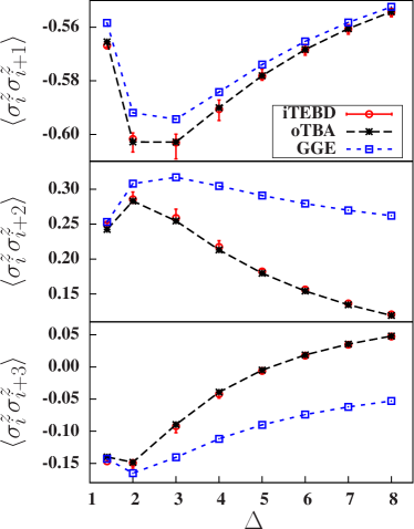
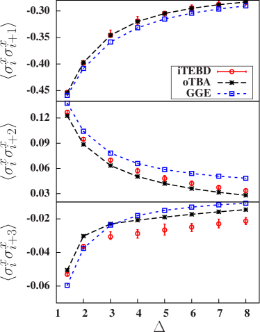
Figure 1: Steady state correlators for quenches starting from the dimer initial state, as a function of the anisotropy parameter $\Delta$.

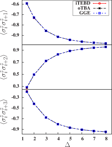
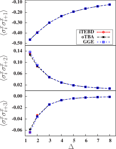
Figure 2: Steady state correlators for quenches starting from the q-dimer initial state, as a function of the anisotropy parameter $\Delta$.

VII Discussion

The conclusion of the present work is the same as that of the previous paper Pozsgay2014 : the GGE fails as a general description for the steady state after quenches in the XXZ spin chain. There are, however, several aspects which need to be examined as a possible explanation for failure. In particular it is necessary to understand how generic the phenomenon is: maybe the failure is due to the particular choice of initial states, or anomalously slow relaxation? Furthermore, is it possible that some more general or different construction for the GGE could be adequate?

VII.1 Steady state ensemble and the role of locality

We recall that the generalized Gibbs ensemble (or, for that matter, thermalization in the non-integrable case) is not expected to describe any observable. Indeed, as the initial state is pure, the exact state of the system given by

$$|\Psi(t)\rangle=e^{-iHt}|\Psi_{0}\rangle$$ (VII.1)

always remains pure. The relaxation towards a thermodynamic state is always understood to work for observables defined on a particular class of subsystems. Let us suppose that the Hilbert space of our system can be written in the “local” form

$$\mathcal{H}=\bigotimes_{x\in S}\mathcal{V}_{x}$$ (VII.2)

where $x$ runs over the system $S$. For a spin chain $x$ labels the spatial location along the chain, but this interpretation is not strictly necessary: “localization” can be true in any other way, e.g. $x$ may label particles composing a many-body system. The important point is that the Hamiltonian governing the dynamics is supposed to be “local”, i.e. sum of terms consisting of product of operators acting on a few adjacent “local” spaces $\mathcal{V}_{x}$, where adjacency is some relation specifying which $x$-s are close to each other. We also suppose that the initial state is the ground state of some other, equally “local” Hamiltonian. The relevant class of observables is then chosen to be the “local” ones, i.e. ones acting on finitely many adjacent $\mathcal{V}_{x}$, and the charges expected to play a role in the steady state statistical operator are the ones that are “local” in the same way as the Hamiltonian is. For the XXZ chain, the notion of $x$-”locality” is just usual spatial locality.

The generalized Gibbs ensemble is defined as a specific thermodynamic and temporal limit, where the order of limits matters. Let us suppose the observable $\mathcal{O}$ is localized in the above sense, i.e. there is a finite subsystem $O$ such that

$$\mathcal{O}\in\bigotimes_{x\in O}L(\mathcal{V}_{x})$$ (VII.3)

where $L(\mathcal{V}_{x})$ are the linear operators on $\mathcal{V}_{x}$; let us call the smallest such subsystem the support of $\mathcal{O}$. Then the statistical operator $\rho_{\mbox{SS}}$ describes the steady state if it is true that

$$\operatorname{Tr}\rho_{\mbox{SS}}\mathcal{O}=\lim_{t\rightarrow\infty}\operatorname{TDL}\,\langle\Psi(t)|\mathcal{O}|\Psi(t)\rangle$$ (VII.4)

where $\operatorname{TDL}$ is the thermodynamic limit in which the size of the system $S$ goes to infinity. In fact it is possible to allow slightly more generality and allow the support of $\mathcal{O}$ to grow in the thermodynamic limit provided the system size becomes infinitely larger than the support of $\mathcal{O}$.

The GGE hypothesis can be stated as

$$\operatorname{Tr}\rho_{\mbox{SS}}\mathcal{O} = \lim_{N\rightarrow\infty}\operatorname{Tr}\rho_{N}\mathcal{O}$$

$$\rho_{N} = \frac{1}{Z_{N}}\exp\!\left(\sum\limits_{k=1}^{N}\beta_{k}Q_{k}\right)\qquad Z_{N}=\operatorname{Tr}\exp\!\left(\sum\limits_{k=1}^{N}\beta_{k}Q_{k}\right)$$ (VII.5)

Note that the GGE is defined above as the limit of the truncated GGE introduced in 2013PhRvB..87x5107F ; Pozsgay2013b . This is motivated by the fact that the infinite sum in the exponent needs some proper definition, especially since including terms up to $N=\infty$ is not really local. It is further justified by the observation that the truncated GGE approximates the full one well; in fact, as described in Subsection III.3.2, charges that are much “larger” than the support of $\mathcal{O}$ do not have much influence on the GGE prediction for the expectation value of $\mathcal{O}$.

The above description generally captures the way the GGE was expected to work for systems with local dynamics such as the XXZ spin chain Pozsgay2013b ; Fagotti2014 . What we have shown is that the GGE defined in the above way definitely fails to describe the steady state of the system.

VII.2 Failure of the Generalized Eigenstate Thermalization Hypothesis

Soon after the results of the papers Wouters2014 ; Pozsgay2014 were made public, work started to explore the mechanism responsible for the failure of the GGE. In Goldstein2014 it was pointed out that the expectation values of the initial charges did not specify the string densities $\rho_{n}$ uniquely. The reason is the existence of multiple types of strings, which means that the elementary magnetic excitations of the XXZ chain, described by 1-strings, have bound states corresponding to longer strings. While the GGE corresponds to maximizing the entropy among configurations allowed by the particular values of the charges specified by the initial state, this does not lead to the same solution that follows from the oTBA, and generally gives different correlations. Indeed this particular point is very interesting, and was investigated further in 2014JSMTE..09..026P . The fact that expectation values of local operators in the thermodynamic limit is not specified by the values of local charges means the failure of the Generalized Eigenstate Thermalization Hypothesis (GETH).

Let us recall how the usual Eigenstate Thermalization Hypothesis works for generic (i.e. non-integrable systems) 1991PhRvA..43.2046D ; 1994PhRvE..50..888S ; 2008Natur.452..854R . As discussed in Subsection III.1, in the large time limit (neglecting degeneracies) one obtains the prediction of the diagonal ensemble (III.5), where each state is weighted by the squared norm of its overlap with the initial state. If the system reaches a thermal equilibrium, then the expectation values of relevant operators should be close to the canonical prediction

$$\left\langle\mathcal{O}\right\rangle_{T}=\frac{\sum_{n}e^{-E_{n}/T}\langle n|\mathcal{O}|n\rangle}{\sum_{n}e^{-E_{n}/T}}$$ (VII.6)

with a temperature $T$ that is fixed by the requirement

$$\left\langle H\right\rangle_{T}=\langle\Psi_{0}|H|\Psi_{0}\rangle\;.$$ (VII.7)

The diagonal ensemble ((III.5)) and the thermal averages (VII.6) are expected to become equal in the $\operatorname{TDL}$. The overlap coefficients entering ((III.5)) are typically random and different from the Boltzmann weights. However, in a large volume $L$ the only states with non-negligible overlap are the ones that have the same energy density as the initial state 2008Natur.452..854R :

$$\frac{E_{n}}{L}\approx\frac{\langle\Psi_{0}|H|\Psi_{0}\rangle}{L}\>,$$ (VII.8)

and the width of the distribution of the energy density goes to zero in the $\operatorname{TDL}$:

$$\Delta\left(\frac{E}{L}\right)=\frac{1}{L}\sqrt{\langle\Psi_{0}|H^{2}|\Psi_{0}\rangle-(\langle\Psi_{0}|H|\Psi_{0}\rangle)^{2}}\sim\frac{1}{\sqrt{L}}\>.$$ (VII.9)

for local Hamiltonians and initial states $\ket{\Psi_{0}}$ satisfying the cluster decomposition principle.

The Eigenstate Thermalization Hypothesis (ETH) 1991PhRvA..43.2046D ; 1994PhRvE..50..888S ; 2008Natur.452..854R states that eigenstates on a given energy shell have almost the same expectation values of physical observables

$$\sum_{n}|c_{n}|^{2}\langle n|\mathcal{O}|n\rangle\approx\left(\sum_{n}|c_{n}|^{2}\right)\langle n_{1}|\mathcal{O}|n_{1}\rangle=\langle n_{1}|\mathcal{O}|n_{1}\rangle\>,$$ (VII.10)

where $n_{1}$ is a reference state satisfying condition (VII.8) and $c_{1}\neq 0$. Recent results 2014arXiv1408.0535K indicate that ((VII.10)) holds in the strict sense that even the largest deviations from the ETH go to zero in the $\operatorname{TDL}$, albeit some local operators may have anomalously slow relaxation rates 2014arXiv1410.4186K . From the ETH it follows that the local observables indeed thermalize:

$$\lim_{t\to\infty}\langle\Psi(t)|\mathcal{O}|\Psi(t)\rangle\approx\left\langle\mathcal{O}\right\rangle_{T}\>,$$ (VII.11)

where the equality is expected to become exact in the $\operatorname{TDL}$.

For integrable systems the steady state was expected to be described by the generalized Gibbs ensemble discussed in Subsection (III.3.2). A possible mechanism for the relaxation to GGE is provided by the Generalized Eigenstate Thermalization Hypothesis (GETH) 2011PhRvL.106n0405C , which states that if all local conserved charges of two different eigenstates are close to each other, then the mean values of local operators are also close. Put differently the values of the conserved charges uniquely determine the correlations in the state; more precisely this is expected to become exact in the $\operatorname{TDL}$. The GETH was checked for a lattice model of hard-core bosons in 2011PhRvL.106n0405C .

However, in 2014JSMTE..09..026P it was shown that the GETH fails in the XXZ spin chain, and it was argued that this is the general case for models with bound states. In Pozsgay2014c it was shown that, on the other hand, the GGE holds in a system of strongly interacting bosons with no bound states. As noted in that work, even though the GGE hypothesis was confirmed, it was not eventually used to describe the steady state. The crucial ingredient was the assumption that the Diagonal Ensemble is valid, plus the fact that there is a one-to-one correspondence between the charges and the root densities, from which the validity of the GGE follows automatically. The steady state correlators were evaluated from the Bethe root density that was obtained directly from the charges using the analogue of the relation (II.20) for the q-boson model, with the GTBA equations described in Subsection (III.3.2) playing no role whatsoever. It seems that this behaviour might be a generic feature of interacting integrable models: the GETH only holds when there is a one-to-one correspondence between the charges and the root densities. In such a case, the GGE density matrix gives the correct steady state correlators for operators whose expectation values depend only on the root densities, since the solution of the GTBA coincides with the unique allowed root densities for the given initial value of the conserved charges.

On the other hand, if the GETH does not hold, then the GTBA analysis of the GGE density matrix is expected to give wrong predictions for a generic initial state. This shows that the failure of the GGE observed in Wouters2014 ; Pozsgay2014 and the present work is not related to the selection of the initial states. In addition, the fact that the oTBA predictions agree with the numerical simulations shows that relaxation to the diagonal ensemble has been achieved in the time frame for which the iTEBD simulations are valid (with the exception of some $\sigma^{x}\sigma^{x}$ correlators, cf. Appendix (B)), and therefore the disagreement with GGE cannot be due to some anomalously slow relaxation.

We remark that our results (see Fig. (3)) are consistent with the observation made in Fagotti2014 that translational invariance is not restored on the observable time scale for quenches starting from the non-translationally invariant dimer state, which affects correlators $\sigma_{i}\sigma_{i+l}$ with $l$ odd. It is possible that translational invariance in these cases is restored on some anomalously long time scale, as argued in Fagotti2014a .

Another interesting observation made in 2014JSMTE..09..026P that the quench action ((III.15)) evaluated at the GGE saddle point solution is infinite, and the spectral weight of the GGE solution (and in fact of all states with thermal asymptotics) decays faster than exponential as a function of the volume. This means that the sum rule ((III.16)) is violated, and the GGE solution is very far from the states selected by the quench action, which actually determine the dynamics of the system.

VII.3 Completeness of the charges and possible extensions of the GGE

The discussion of the GETH shows that one way to construct the correct ensemble is to find charges which fix all Bethe root densities to their correct values, thus making the GGE complete and correct. In this work the GGE was constructed using the local charges obtained as derivatives of the transfer matrix.

However, new quasi-local operators have been found recently for the regime $\Delta<1$ 2011PhRvL.106u7206P ; 2014NuPhB.886.1177P ; 2014JSMTE..09..037P and it is interesting open question whether the addition of these new operators to the GGE is enough to fix all root densities to their correct values, thus obtaining an extended GGE which can describe the steady state after the quantum quench. Unfortunately the construction of 2011PhRvL.106u7206P ; 2014NuPhB.886.1177P ; 2014JSMTE..09..037P does not produce quasi-local operators for $\Delta>1$, and it remains to be seen whether new charges can be produced by other means in this regime.

It is also important to keep in mind that consistency of a thermodynamic description requires extensivity of the charges involved in the ensemble. Locality is one way of ensuring extensivity, but more general (e.g. quasi-local) charges could be suitable for inclusion into a thermodynamic ensemble. In free systems, for example, the GGE is usually formulated in terms of the mode occupation numbers, which are non-local quantities.

Recently the extension of the GGE by quasi-local charges was considered for quantum field theories; however, the charges discussed in 2014arXiv1411.5352E are already included in our set of local charges at the level of the discrete chain. At present it is an open question whether there exists a set of charges, possibly including quasi-local ones that would be complete in the sense of fixing the root densities. In the light of recent interest in experimental observation of the GGE 2014arXiv1411.7185L it would also be preferable if the extension preserved the truncatability of the GGE (cf. 2013JSMTE..07..003P , see also Subsections III.3.2 and VII.1), namely that truncation to a small subset of charges would give a reasonable approximation for the exact result, so that fitting the ensemble to measurements would only require a small number of parameters.

Acknowledgments

We would like to thank M. Kormos and G. Zaránd for numerous discussions, their valuable feedback, and F. Pollmann and P. Moca for the help they gave us to set up the iTEBD calculations. We are grateful to J.-S. Caux, J. De Nardis, and B. Wouters for useful discussions on their work, and for sharing some of their numerical data with us. M.A.W. acknowledges financial support from Hungarian Grants No. K105149 and CNK80991.

Appendix A Mean values of correlators: decoupling the equations

In this appendix we show that the partially decoupled equations (V.1-2), which first appeared in 2014JSMTE..09..026P , are indeed equivalent to the original coupled equations of Mestyan2014 , which read

$$\rho_{n}^{(j)}(\lambda) = a_{n}^{(j)}(\lambda)-\sum_{m=1}^{\infty}T_{nm}\star\frac{\rho_{m}^{(j)}}{1+\eta_{m}}$$ (A.1)

$$\sigma_{n}^{(j)}(\lambda) = -b_{n}^{(j)}(\lambda)+\sum_{m=1}^{\infty}U_{nm}\star\frac{\rho_{m,\mbox{t}}^{(j)}}{1+\eta_{m}}-\sum_{m=1}^{\infty}T_{nm}\star\frac{\sigma_{m}^{(j)}}{1+\eta_{m}}\,,$$ (A.2)

with the convolution kernels being

$$T_{nm}=(1-\delta_{n,m})a_{|n-m|}+a_{n+m}+2\sum_{j=1}^{\min(n,m)-1}a_{|n-m|+2j}$$

$$U_{nm}=(1-\delta_{n,m})b_{|n-m|}+b{}_{n+m}+2\sum_{j=1}^{\min(n,m)-1}b_{|n-m|+2j}\,,$$

and the source terms being

$$a_{n}^{(j)}(\lambda) = \left(\frac{d}{d\lambda}\right)^{j}a_{n}(\lambda)$$ (A.3)

$$b_{n}(\lambda) = \frac{1}{2\pi}i\frac{d}{d\eta}\log\left(\frac{\sin(\lambda+in\eta/2)}{\sin(\lambda-in\eta/2)}\right)=-\frac{n}{2\pi}\frac{\sin(2\lambda)}{\cosh n\eta-\cos(2\lambda)}\frac{\sigma_{n+1}^{(j)}}{1+1/\eta_{n+1}}$$

$$b_{n}^{(j)}(\lambda) = \left(\frac{d}{d\lambda}\right)^{j}b_{n}(\lambda)\,,$$ (A.4)

where $a_{n}(\lambda)$ is defined by (II.10).

In order to prove the equivalence of (A.1-A.4) to (V.1-2), it is convenient to introduce the following notations for the Fourier transform

$$\tilde{f}(k)=(\mathcal{F}f)(k)=\int_{-\pi/2}^{\pi/2}d\lambda f(\lambda)e^{2ik\lambda}\qquad k\in\mathbb{Z}\,.$$

For $k\in\mathbb{Z},$ $\tilde{f}(k)$ is the $k$-th Fourier coefficient of $f$:

$$f(\lambda)=(\mathcal{F}^{-1}\tilde{f})(\lambda)=\frac{1}{\pi}\sum_{k\in\mathbb{Z}}\tilde{f}(k)e^{-2ik\lambda}.$$

The Fourier transforms of the functions (A.3) are given by

$$\tilde{a}_{n}^{(j)}(k)=(-2ik)^{j}e^{-n\eta|k|},$$

while the Fourier transforms of (A.4) have the form

$$\tilde{b}_{n}^{(j)}(k)=\frac{-in\operatorname{sgn}(k)(-2ik)^{j}}{2}e^{-n\eta|k|}=\frac{i}{2\eta}\frac{d}{dk}\tilde{a}_{n}^{(j)}(k)-\frac{j}{2\eta}\tilde{a}_{n}^{(j-1)}(k)\,,$$ (A.5)

where $\operatorname{sgn}(0)=0$ and $\operatorname{sgn}(x)=x/|x|$ for $x\neq 0$. Although (A.3) and (A.4) define $a_{n}(\lambda)$ and $b_{n}(\lambda)$ for $n>1$ only, it is useful to define $\tilde{a}_{0}^{(j)}(k)$ and $\tilde{b}_{0}^{(j)}(k)$ by extending the equations to $n=0$. We also define $\tilde{a}_{n}(k)=\tilde{a}_{n}^{(0)}(k)$ and $\tilde{b}_{n}(k)=\tilde{b}_{n}^{(0)}(k)$.

Using the above notations, the Fourier transforms of the coupled equations (A.1-A.2) are the following

$$\rho_{n}^{(j)}(k) = \tilde{a}_{n}^{(j)}(k)-\sum_{m=1}^{\infty}\tilde{T}_{nm}(k)\left(\mbox{$\mathcal{F}$}\frac{\rho_{m}^{(j)}}{1+\eta_{m}}\right)(k)$$ (A.6)

$$\sigma_{n}^{(j)}(k) = -\tilde{b_{n}}^{(j)}(k)+\sum_{m=1}^{\infty}\tilde{U}_{nm}(k)\left(\mathcal{F}\frac{\rho_{m}^{(j)}}{1+\eta_{m}}\right)(k)-\sum_{m=1}^{\infty}\tilde{T}_{nm}(k)\left(\mathcal{F}\frac{\sigma_{m}^{(j)}}{1+\eta_{m}}\right)(k)\,.$$ (A.7)

The decoupled form of (A.6) is obtained by subtracting the sum of $n-1$th and $n+1$th equations multiplied by $\tilde{a}_{1}(k)$, from the $n$th equation multiplied by $\tilde{a}_{0}(k)+\tilde{a}_{2}(k)$:

$$(\tilde{a}_{0}(k)+\tilde{a}_{2}(k))\rho_{n}^{(j)}(k)=\tilde{a}_{1}(k)\delta_{n,1}+\tilde{a}_{1}(k)\left[\left(\mathcal{F}\frac{\rho_{n-1}^{(j)}}{1+1/\eta_{n-1}}\right)(k)+\left(\mathcal{F}\frac{\rho_{n+1}^{(j)}}{1+1/\eta_{n+1}}\right)(k)\right]\,.$$ (A.8)

Introducing

$$\tilde{s}(k)=\frac{1}{\tilde{a}_{1}(k)+\tilde{a}_{-1}(k)}$$

we obtain

$$\tilde{\rho}_{n}^{(j)}(k)=\tilde{s}(k)\delta_{n,1}+\tilde{s}(k)\left[\left(\mathcal{F}\frac{\rho_{n-1}^{(j)}}{1+1/\eta_{n-1}}\right)(k)+\left(\mathcal{F}\frac{\rho_{n+1}^{(j)}}{1+1/\eta_{n+1}}\right)(k)\right]\,,$$

which is the Fourier transform of the partially decoupled equation (V.1).

Decoupling (A.7) proceeds via a relation between the Fourier transforms of the convolution kernels $\tilde{T}_{nm}(k)$ and $\tilde{U}_{nm}(k)$ similar to (A.5):

$$\tilde{U}_{nm}(k)=\frac{i}{2\eta}\frac{d}{dk}\tilde{T}_{nm}(k)\,.$$ (A.9)

Acting with $(i/2\eta)(d/dk)$ on (A.6), we obtain

$$0= \frac{i}{2\eta}\frac{d}{d(k)}\tilde{a}_{n}(k)-\sum_{m=1}^{\infty}\frac{i}{2\eta}\left(\frac{d}{dk}\tilde{T}_{nm}(k)\right)\left(\mathcal{F}\frac{\rho_{m}^{(j)}}{1+\eta_{m}}\right)(k)-$$ (A.10)

$$- \frac{i}{2\eta}\left[\frac{d}{dk}\rho_{n}^{(j)}(k)+\sum_{m=1}^{\infty}\tilde{T}_{nm}(k)\frac{d}{dk}\left(\mathcal{F}\frac{\rho_{m}^{(j)}}{1+\eta_{m}}\right)(k)\right]\,.$$

Using the relations (A.5) and (A.9) on (A.7), we get

$$\sigma_{n}^{(j)}(k) =-\frac{i}{2\eta}\frac{d}{d(k)}\tilde{a}_{n}(k)+\sum_{m=1}^{\infty}\frac{i}{2\eta}\left(\frac{d}{dk}\tilde{T}_{nm}(k)\right)\left(\mathcal{F}\frac{\rho_{m}^{(j)}}{1+\eta_{m}}\right)(k)+$$ (A.11)

$$+\frac{j}{2\eta}\tilde{a}_{n}^{(j-1)}(k)-\sum_{m=1}^{\infty}\tilde{T}_{nm}(k)\left(\mathcal{F}\frac{\sigma_{m}^{(j)}}{1+\eta_{m}}\right)(k)\,.$$

Substituting the first two terms of (A.11) with the third term of (A.10) yields

$$\sigma_{n}^{(j)}(k) =-\frac{i}{2\eta}\left[\frac{d}{dk}\rho_{n}^{(j)}(k)+\sum_{m=1}^{\infty}\tilde{T}_{nm}(k)\frac{d}{dk}\left(\mathcal{F}\frac{\rho_{m}^{(j)}}{1+\eta_{m}}\right)(k)\right]+$$ (A.12)

$$+\frac{j}{2\eta}\tilde{a}_{n}^{(j-1)}(k)-\sum_{m=1}^{\infty}\tilde{T}_{nm}(k)\left(\mathcal{F}\frac{\sigma_{m}^{(j)}}{1+\eta_{m}}\right)(k).$$

Now the system (A.12) is easily decoupled, similarly to (A.6). Subtracting the sum of $n-1$th and $n+1$th equations multiplied by $\tilde{a}_{1}(k)$, from the $n$th equation multiplied by $\tilde{a}_{0}(k)+\tilde{a}_{2}(k)$ leads to

$$(\tilde{a}_{0}(k)+\tilde{a}_{2}(k))\tilde{\sigma}_{n}^{(j)}(k) =-\frac{i}{2\eta}\Bigg{\{}(\tilde{a}_{0}(k)+\tilde{a}_{2}(k))\frac{d}{dk}\tilde{\rho}_{n}^{(j)}(k)\,-$$ (A.13)

$$-\tilde{a}_{1}(k)\left[\frac{d}{dk}\tilde{\rho}_{n-1}^{(j)}(k)+\frac{d}{dk}\tilde{\rho}_{n+1}^{(j)}(k)\right]+$$

$$+\tilde{a}_{1}(k)\left[\frac{d}{dk}\left(\mathcal{F}\frac{\rho_{n-1}^{(j)}}{1+\eta_{n-1}}\right)(k)+\frac{d}{dk}\left(\mathcal{F}\frac{\rho_{n+1}^{(j)}}{1+\eta_{n+1}}\right)(k)\right]\Bigg{\}}\,+$$

$$+\frac{j}{2\eta}\tilde{a}_{1}^{(j-1)}(k)\delta_{n,1}\,+$$

$$+\tilde{a}_{1}(k)\left[\left(\mathcal{F}\frac{\sigma_{n-1}^{(j)}}{1+1/\eta_{n-1}}\right)(k)+\left(\mathcal{F}\frac{\sigma_{n+1}^{(j)}}{1+1/\eta_{n+1}}\right)(k)\right]\,.$$

This system is already partially decoupled like (A.8) but it can be simplified even further. Rearranging the terms in the curly brackets leads to

$$(\tilde{a}_{0}+\tilde{a}_{2})\sigma_{n}(k) =-\frac{i}{2\eta}\Bigg{\{}(\tilde{a}_{0}(k)+\tilde{a}_{2}(k))\frac{d}{dk}\rho_{n}^{(j)}(k)-$$ (A.14)

$$-\tilde{a}_{1}(k)\left[\frac{d}{dk}\left(\mathcal{F}\frac{\rho_{n-1}^{(j)}}{1+1/\eta_{n-1}}\right)(k)+\,\frac{d}{dk}\left(\mathcal{F}\frac{\rho_{n+1}^{(j)}}{1+1/\eta_{n+1}}\right)(k)\right]\Bigg{\}}\,+$$

$$+\frac{j}{2\eta}\tilde{a}_{1}^{(j-1)}(k)\delta_{n,1}\,+$$

$$+\tilde{a}_{1}(k)\left[\left(\mathcal{F}\frac{\sigma_{n-1}^{(j)}}{1+1/\eta_{n-1}}\right)(k)+\left(\mathcal{F}\frac{\sigma_{n+1}^{(j)}}{1+1/\eta_{n+1}}\right)(k)\right]\,.$$

Using the Leibniz rule $f(dg/dk)=d(fg)/dk-(df/dk)g$ and formula (A.8), the expression between the curly brackets can be written as

$$\left[\frac{d}{d(k)}\tilde{a}_{1}^{(j)}(k)-\tilde{a}_{1}^{(j)}(k)\frac{\frac{d}{dk}\tilde{a}_{0}(k)+\frac{d}{dk}\tilde{a}_{2}(k)}{\tilde{a}_{0}(k)+\tilde{a}_{2}(k)}\right]\delta_{n,1}+$$

$$+ \left[\frac{d}{d(k)}\tilde{a}_{1}(k)-\tilde{a}_{1}(k)\frac{\frac{d}{dk}\tilde{a}_{0}(k)+\frac{d}{dk}\tilde{a}_{2}(k)}{\tilde{a}_{0}(k)+\tilde{a}_{2}(k)}\right]\left[\left(\mathcal{F}\frac{\rho_{n-1}^{(j)}}{1+1/\eta_{n-1}}\right)(k)+\left(\mathcal{F}\frac{\rho_{n+1}^{(j)}}{1+1/\eta_{n+1}}\right)(k)\right]\,.$$

Introducing the notation

$$\tilde{t}^{(j)}(k) =-\frac{\tilde{b}_{1}^{(j)}(k)-\tilde{a}_{1}^{(j)}(k)\frac{\tilde{b}_{0}(k)+\tilde{b}_{2}(k)}{\tilde{a}_{0}(k)+\tilde{a}_{2}(k)}}{\tilde{a}_{0}(k)+\tilde{a}_{2}(k)}=\frac{i(-2ik)^{j}}{2}\frac{e^{\eta|k|}-e^{-\eta|k|}}{(e^{\eta|k|}+e^{-\eta|k|})^{2}}$$

the system (A.14) transforms to

$$\tilde{\sigma}_{n}^{(j)}(k) = \delta_{n,1}\tilde{t}^{(j)}(k)+\tilde{t}(k)\left[\mathcal{F}\left(\frac{\rho_{n-1}^{(j)}}{1+1/\eta_{n-1}}\right)(k)+\left(\mathcal{F}\frac{\rho_{n+1}^{(j)}}{1+1/\eta_{n+1}}\right)(k)\right]+$$

$$+ \tilde{s}(k)\left[\left(\mathcal{F}\frac{\sigma_{n-1}^{(j)}}{1+1/\eta_{n-1}}\right)(k)+\left(\mathcal{F}\frac{\sigma_{n+1}^{(j)}}{1+1/\eta_{n+1}}\right)(k)\right],$$

which is precisely the Fourier transform of the system (2).

Finally, formulas (V.3) can be obtained directly from their coupled counterparts Mestyan2014

$$\Omega_{j,l} =4\pi\sum_{n=1}^{\infty}\int_{-\pi/2}^{\pi/2}d\lambda a_{n}^{(l)}(\lambda)\frac{\rho_{n}^{(j)}(\lambda)}{1+\eta_{n}(\lambda)}$$

$$\Gamma_{j,l} =-4\pi\sum_{n=1}^{\infty}\int_{-\pi/2}^{\pi/2}d\lambda\left(b_{n}^{(l)}(\lambda)\frac{\rho^{(j)}(\lambda)}{1+\eta_{n}(\lambda)}+a_{n}^{(l)}(\lambda)\frac{\sigma^{(j)}(\lambda)}{1+\eta_{n}(\lambda)}\right)$$

by using the partially decoupled equations (V.1-2).

Appendix B Details of iTEBD simulations

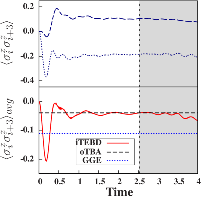
Figure 3: The upper panel shows the relaxation of the $\langle\sigma_{i}^{z}\sigma_{i+3}^{z}\rangle$ correlator in the two sublattices, calculated by the iTEBD algorithm. The simulation was started from the dimer state and the anisotropy parameter was set to $\Delta=4$. In the shaded region the simulation is unreliable because of the truncation error. The translational invariance is not restored in the achievable timescale of the iTEBD simulation. The lower panel shows the relaxation of the sublattice averaged correlator calculated by the iTEBD code (continuous red line). The blue dotted line shows the GGE prediction, while the dashed black line represents the oTBA prediction. The GGE result deviates strongly from the iTEBD simulations. The oTBA prediction, however, describes the stationary value with high precision.

The real time dynamics of the spin chains were numerically simulated using the Infinite-size Time Evolving Block Decimation (iTEBD) algorithm developed in 2004PhRvL..93d0502V ; 2007PhRvL..98g0201V . In this algorithm the state of the system is approximated by a matrix product state (MPS) 2011AnPhy.326…96S , and the time-evolution is approximated in a Suzuki-Trotter expansion by consecutive two-site evolution steps. In the calculations the rotational symmetry around the $z$-axis was exploited by introducing the conserved charge – the $z$-component of the total spin – and performing the time steps for the different charge blocks separately.

The precision of the MPS Ansatz can be controlled by the dimensions of the matrices. The required sizes depend strongly on the entanglement between separate parts of the system. In a real time simulation of an infinite system, the entanglement of the simulated state grows rapidly. The required MPS-dimension ($\chi$) grows exponentially that results in a threshold, where the simulation loses its reliability. Due to the exponential growth, the threshold time can only slowly move by increasing $\chi$.

In our calculations maximal dimensions of the U(1) blocks were set to $\chi_{block}=400-800$ resulting in a total matrix dimension $\chi_{tot}>1200-2400$. In the time-evolution a first order Suzuki-Trotter expansion was used with a time-step $dt=0.001$. We tested the reliability of discretization by changing the time-step and found that decreasing $dt$ does not modify our results.

The $\langle\sigma_{i}^{x}\sigma_{j}^{x}\rangle$ and $\langle\sigma_{i}^{z}\sigma_{j}^{z}\rangle$ correlations were calculated at each time step up to third neighbour distance. Preparing the system in the dimer and q-dimer states – in contrast with the Néel state – these correlations are not invariant under translations by the lattice constant. In the Fig. 3 the $\langle\sigma_{i}^{z}\sigma_{i+3}^{z}\rangle$ correlator is shown when the relaxation starts from the dimer state. The translational invariance is not restored in the achievable simulation times and it is still an open question whether it is restored in the $t\rightarrow\infty$ limit or not. The sublattice averaged correlator, however, converge rapidly to a stationary value that is equal to the oTBA prediction within the numerical errors.

To extract the stationary correlators from the iTEBD simulations we defined the threshold of the simulation at the time where the one-step truncated weight exceeds $10^{-8}$. As an alternative method we ran the code with different matrix dimensions and determined the time where the results deviated upon increasing matrix dimension. The two methods resulted approximately in the same threshold time. Because we do not have any reliable analytic expression for the real-time evolution of the correlators, the estimated stationary values were calculated by simple time averaging for the last $\Delta T=1$ time window before the threshold. The error bars were estimated by the minimal and maximal values within the time window. The method works well in the case of $zz$-correlators (see Fig. 3), where the correlator rapidly converge to the stationary value. In that case the amplitude of small oscillations gives a reasonable error-bar. In the case of $xx$-correlators, however, the convergence is much slower (see Fig. 4). The correlator slowly drifts towards a stationary value but does not reach it before the threshold. In the case of such a slow drift, the estimation of error bars with minimal and maximal values in the time window is not optimal, because it can not quantify how far the real stationary value is.

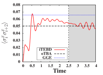
Figure 4: The relaxation of the $\langle\sigma_{i}^{x}\sigma_{i+2}^{x}\rangle$ correlator is shown (red continuous line). The simulation was started from the dimer state, and the anisotropy parameter was set to $\Delta=4$. The blue dotted line shows the GGE prediction, while the dashed black line represents the oTBA prediction. Compared to the $zz$ correlator (see Fig. 3) the relaxation is much slower. Because of the slow drift an accurate extrapolation for the stationary value was not possible.

References

- (1) A. Polkovnikov, K. Sengupta, A. Silva, and M. Vengalattore, “Colloquium: Nonequilibrium dynamics of closed interacting quantum systems,” Reviews of Modern Physics 83 (July, 2011) 863–883, arXiv:1007.5331 [cond-mat.stat-mech].
- (2) C. Kollath, A. M. Läuchli, and E. Altman, “Quench Dynamics and Nonequilibrium Phase Diagram of the Bose-Hubbard Model,” Physical Review Letters 98 no. 18, (May, 2007) 180601, cond-mat/0607235.
- (3) M. Rigol, V. Dunjko, and M. Olshanii, “Thermalization and its mechanism for generic isolated quantum systems,” Nature (London) 452 (Apr., 2008) 854–858, arXiv:0708.1324 [cond-mat.stat-mech].
- (4) T. Barthel and U. Schollwöck, “Dephasing and the Steady State in Quantum Many-Particle Systems,” Physical Review Letters 100 no. 10, (Mar., 2008) 100601, arXiv:0711.4896 [cond-mat.stat-mech].
- (5) M. Rigol, “Breakdown of Thermalization in Finite One-Dimensional Systems,” Physical Review Letters 103 no. 10, (Sept., 2009) 100403, arXiv:0904.3746 [cond-mat.stat-mech].
- (6) M. Cramer and J. Eisert, “A quantum central limit theorem for non-equilibrium systems: exact local relaxation of correlated states,” New Journal of Physics 12 no. 5, (May, 2010) 055020, arXiv:0911.2475 [quant-ph].
- (7) L. F. Santos and M. Rigol, “Onset of quantum chaos in one-dimensional bosonic and fermionic systems and its relation to thermalization,” Phys. Rev. E 81 no. 3, (Mar., 2010) 036206, arXiv:0910.2985 [cond-mat.stat-mech].
- (8) P. Barmettler, M. Punk, V. Gritsev, E. Demler, and E. Altman, “Quantum quenches in the anisotropic spin-frac12 Heisenberg chain: different approaches to many-body dynamics far from equilibrium,” New Journal of Physics 12 no. 5, (May, 2010) 055017, arXiv:0911.1927 [cond-mat.quant-gas].
- (9) M. C. Bañuls, J. I. Cirac, and M. B. Hastings, “Strong and Weak Thermalization of Infinite Nonintegrable Quantum Systems,” Physical Review Letters 106 no. 5, (Feb., 2011) 050405, arXiv:1007.3957 [quant-ph].
- (10) P. Calabrese, F. H. L. Essler, and M. Fagotti, “Quantum Quench in the Transverse-Field Ising Chain,” Physical Review Letters 106 no. 22, (June, 2011) 227203, arXiv:1104.0154 [cond-mat.str-el].
- (11) P. Calabrese, F. H. L. Essler, and M. Fagotti, “Quantum quench in the transverse field Ising chain: I. Time evolution of order parameter correlators,” Journal of Statistical Mechanics: Theory and Experiment 7 (July, 2012) 16, arXiv:1204.3911 [cond-mat.quant-gas].
- (12) N. Sedlmayr, J. Ren, F. Gebhard, and J. Sirker, “Closed and Open System Dynamics in a Fermionic Chain with a Microscopically Specified Bath: Relaxation and Thermalization,” Physical Review Letters 110 no. 10, (Mar., 2013) 100406, arXiv:1212.0223 [cond-mat.stat-mech].
- (13) M. Marcuzzi, J. Marino, A. Gambassi, and A. Silva, “Prethermalization in a Nonintegrable Quantum Spin Chain after a Quench,” Physical Review Letters 111 no. 19, (Nov., 2013) 197203, arXiv:1307.3738 [cond-mat.stat-mech].
- (14) D. Iyer, H. Guan, and N. Andrei, “Exact formalism for the quench dynamics of integrable models,” Phys. Rev. A 87 no. 5, (May, 2013) 053628, arXiv:1304.0506 [cond-mat.quant-gas].
- (15) T. Kinoshita, T. Wenger, and D. S. Weiss, “A quantum Newton’s cradle,” Nature (London) 440 (Apr., 2006) 900–903.
- (16) M. Cheneau, P. Barmettler, D. Poletti, M. Endres, P. Schauß, T. Fukuhara, C. Gross, I. Bloch, C. Kollath, and S. Kuhr, “Light-cone-like spreading of correlations in a quantum many-body system,” Nature (London) 481 (Jan., 2012) 484–487, arXiv:1111.0776 [cond-mat.quant-gas].
- (17) S. Trotzky, Y.-A. Chen, A. Flesch, I. P. McCulloch, U. Schollwöck, J. Eisert, and I. Bloch, “Probing the relaxation towards equilibrium in an isolated strongly correlated one-dimensional Bose gas,” Nature Physics 8 (Apr., 2012) 325–330, arXiv:1101.2659 [cond-mat.quant-gas].
- (18) T. Fukuhara, P. Schauß, M. Endres, S. Hild, M. Cheneau, I. Bloch, and C. Gross, “Microscopic observation of magnon bound states and their dynamics,” Nature (London) 502 (Oct., 2013) 76–79, arXiv:1305.6598 [cond-mat.quant-gas].
- (19) M. Rigol, V. Dunjko, V. Yurovsky, and M. Olshanii, “Relaxation in a Completely Integrable Many-Body Quantum System: An AbInitio Study of the Dynamics of the Highly Excited States of 1D Lattice Hard-Core Bosons,” Physical Review Letters 98 no. 5, (Feb., 2007) 050405, cond-mat/0604476.
- (20) V. E. Korepin, N. M. Bogoliubov, and A. G. Izergin, Quantum Inverse Scattering Method and Correlation Functions. Cambridge University Press, Cambridge, 1993.
- (21) M. A. Cazalilla, “Effect of Suddenly Turning on Interactions in the Luttinger Model,” Physical Review Letters 97 no. 15, (Oct., 2006) 156403, cond-mat/0606236.
- (22) D. Rossini, A. Silva, G. Mussardo, and G. E. Santoro, “Effective Thermal Dynamics Following a Quantum Quench in a Spin Chain,” Physical Review Letters 102 no. 12, (Mar., 2009) 127204, arXiv:0810.5508 [cond-mat.stat-mech].
- (23) P. Calabrese, F. H. L. Essler, and M. Fagotti, “Quantum quenches in the transverse field Ising chain: II. Stationary state properties,” Journal of Statistical Mechanics: Theory and Experiment 7 (July, 2012) 22, arXiv:1205.2211 [cond-mat.stat-mech].
- (24) M. A. Cazalilla, A. Iucci, and M.-C. Chung, “Thermalization and quantum correlations in exactly solvable models,” Phys. Rev. E 85 no. 1, (Jan., 2012) 011133, arXiv:1106.5206 [cond-mat.stat-mech].
- (25) V. Gurarie, “Global large time dynamics and the generalized Gibbs ensemble,” Journal of Statistical Mechanics: Theory and Experiment 2 (Feb., 2013) 14, arXiv:1209.3816 [cond-mat.stat-mech].
- (26) M. Fagotti and F. H. L. Essler, “Reduced density matrix after a quantum quench,” Phys. Rev. B 87 no. 24, (June, 2013) 245107, arXiv:1302.6944 [cond-mat.stat-mech].
- (27) M. Fagotti, “On conservation laws, relaxation and pre-relaxation after a quantum quench,” Journal of Statistical Mechanics: Theory and Experiment 3 (Mar., 2014) 16, arXiv:1401.1064 [cond-mat.stat-mech].
- (28) M. Collura, S. Sotiriadis, and P. Calabrese, “Equilibration of a Tonks-Girardeau Gas Following a Trap Release,” Physical Review Letters 110 no. 24, (June, 2013) 245301, arXiv:1303.3795 [cond-mat.quant-gas].
- (29) M. Kormos, M. Collura, and P. Calabrese, “Analytic results for a quantum quench from free to hard-core one-dimensional bosons,” Phys. Rev. A 89 no. 1, (Jan., 2014) 013609, arXiv:1307.2142 [cond-mat.quant-gas].
- (30) S. Sotiriadis and P. Calabrese, “Validity of the GGE for quantum quenches from interacting to noninteracting models,” Journal of Statistical Mechanics: Theory and Experiment 7 (July, 2014) 24, arXiv:1403.7431 [cond-mat.stat-mech].
- (31) A. C. Cassidy, C. W. Clark, and M. Rigol, “Generalized Thermalization in an Integrable Lattice System,” Physical Review Letters 106 no. 14, (Apr., 2011) 140405, arXiv:1008.4794 [cond-mat.stat-mech].
- (32) T. M. Wright, M. Rigol, M. J. Davis, and K. V. Kheruntsyan, “Nonequilibrium Dynamics of One-Dimensional Hard-Core Anyons Following a Quench: Complete Relaxation of One-Body Observables,” Physical Review Letters 113 no. 5, (Aug., 2014) 050601, arXiv:1312.4657 [cond-mat.quant-gas].
- (33) J.-S. Caux and R. M. Konik, “Constructing the Generalized Gibbs Ensemble after a Quantum Quench,” Physical Review Letters 109 no. 17, (Oct., 2012) 175301, arXiv:1203.0901 [cond-mat.quant-gas].
- (34) M. Kormos, A. Shashi, Y.-Z. Chou, J.-S. Caux, and A. Imambekov, “Interaction quenches in the one-dimensional Bose gas,” Phys. Rev. B 88 no. 20, (Nov., 2013) 205131, arXiv:1305.7202 [cond-mat.stat-mech].
- (35) J. De Nardis, B. Wouters, M. Brockmann, and J.-S. Caux, “Solution for an interaction quench in the Lieb-Liniger Bose gas,” Phys. Rev. A 89 no. 3, (Mar., 2014) 033601, arXiv:1308.4310 [cond-mat.stat-mech].
- (36) B. Pozsgay, “The generalized Gibbs ensemble for Heisenberg spin chains,” Journal of Statistical Mechanics: Theory and Experiment 7 (July, 2013) 3, arXiv:1304.5374 [cond-mat.stat-mech].
- (37) M. Fagotti and F. H. L. Essler, “Stationary behaviour of observables after a quantum quench in the spin-1/2 Heisenberg XXZ chain,” Journal of Statistical Mechanics: Theory and Experiment 7 (July, 2013) 12, arXiv:1305.0468 [cond-mat.stat-mech].
- (38) M. Fagotti, M. Collura, F. H. L. Essler, and P. Calabrese, “Relaxation after quantum quenches in the spin-1/2 Heisenberg XXZ chain,” Phys. Rev. B 89 no. 12, (Mar., 2014) 125101, arXiv:1311.5216 [cond-mat.stat-mech].
- (39) D. Fioretto and G. Mussardo, “Quantum quenches in integrable field theories,” New Journal of Physics 12 no. 5, (May, 2010) 055015, arXiv:0911.3345 [cond-mat.stat-mech].
- (40) G. Mussardo, “Infinite-Time Average of Local Fields in an Integrable Quantum Field Theory After a Quantum Quench,” Physical Review Letters 111 no. 10, (Sept., 2013) 100401, arXiv:1308.4551 [cond-mat.stat-mech].
- (41) S. Sotiriadis, G. Takacs, and G. Mussardo, “Boundary state in an integrable quantum field theory out of equilibrium,” Physics Letters B 734 (June, 2014) 52–57, arXiv:1311.4418 [cond-mat.stat-mech].
- (42) J.-S. Caux and F. H. L. Essler, “Time Evolution of Local Observables After Quenching to an Integrable Model,” Physical Review Letters 110 no. 25, (June, 2013) 257203, arXiv:1301.3806.
- (43) K. K. Kozlowski and B. Pozsgay, “Surface free energy of the open XXZ spin-1/2 chain,” Journal of Statistical Mechanics: Theory and Experiment 5 (May, 2012) 21, arXiv:1201.5884 [nlin.SI].
- (44) B. Pozsgay, “Overlaps between eigenstates of the XXZ spin-1/2 chain and a class of simple product states,” Journal of Statistical Mechanics: Theory and Experiment 2014 no. 6, (June, 2014) P06011.
- (45) M. Brockmann, J. De Nardis, B. Wouters, and J.-S. Caux, “A Gaudin-like determinant for overlaps of Néel and XXZ Bethe states,” Journal of Physics A Mathematical General 47 no. 14, (Apr., 2014) 145003, arXiv:1401.2877 [cond-mat.stat-mech].
- (46) M. Brockmann, “Overlaps of q -raised Néel states with XXZ Bethe states and their relation to the Lieb–Liniger Bose gas,” Journal of Statistical Mechanics: Theory and Experiment 2014 no. 5, (May, 2014) P05006, arXiv:1402.1471.
- (47) B. Wouters, J. De Nardis, M. Brockmann, D. Fioretto, M. Rigol, and J.-S. Caux, “Quenching the Anisotropic Heisenberg Chain: Exact Solution and Generalized Gibbs Ensemble Predictions,” Physical Review Letters 113 no. 11, (Sept., 2014) 117202, arXiv:1405.0172.
- (48) B. Pozsgay, M. Mestyán, M. A. Werner, M. Kormos, G. Zaránd, and G. Takács, “Correlations after Quantum Quenches in the XXZ Spin Chain: Failure of the Generalized Gibbs Ensemble,” Physical Review Letters 113 no. 11, (Sept., 2014) 117203.
- (49) G. Vidal, “Efficient Simulation of One-Dimensional Quantum Many-Body Systems,” Physical Review Letters 93 no. 4, (July, 2004) 040502, quant-ph/0310089.
- (50) G. Vidal, “Classical Simulation of Infinite-Size Quantum Lattice Systems in One Spatial Dimension,” Physical Review Letters 98 no. 7, (Feb., 2007) 070201, cond-mat/0605597.
- (51) M. Mestyán and B. Pozsgay, “Short distance correlators in the XXZ spin chain for arbitrary string distributions,” Journal of Statistical Mechanics: Theory and Experiment 2014 no. 9, (Sept., 2014) P09020, arXiv:1405.0232.
- (52) B. Pozsgay, “The dynamical free energy and the Loschmidt echo for a class of quantum quenches in the Heisenberg spin chain,” Journal of Statistical Mechanics: Theory and Experiment 2013 no. 10, (Oct., 2013) P10028.
- (53) G. Goldstein and N. Andrei, “Failure of the GGE hypothesis for integrable models with bound states,” arXiv:1405.4224.
- (54) B. Pozsgay, “Failure of the generalized eigenstate thermalization hypothesis in integrable models with multiple particle species,” Journal of Statistical Mechanics: Theory and Experiment 9 (Sept., 2014) 26, arXiv:1406.4613 [cond-mat.stat-mech].
- (55) B. Pozsgay, “Quantum quenches and Generalized Gibbs Ensemble in a Bethe Ansatz solvable lattice model of interacting bosons,” arXiv:1407.8344.
- (56) H. A. Bethe, “Zur Theorie der Metalle; 1, Eigenwerte und Eigenfunktionen der linearen Atomkette,” Z. Phys. 71 (1931) 205–226.
- (57) R. Orbach, “Linear antiferromagnetic chain with anisotropic coupling,” Physical Review 112 (1958) 309–316.
- (58) M. Takahashi, Thermodynamics of One-Dimensional Solvable Models. Cambridge University Press, Cambridge, 1999.
- (59) M. P. Grabowski and P. Mathieu, “Quantum Integrals of Motion for the Heisenberg Spin Chain,” Modern Physics Letters A 9 (1994) 2197–2206, hep-th/9403149.
- (60) M. Brockmann, B. Wouters, D. Fioretto, J. De Nardis, R. Vlijm, and J.-S. Caux, “Quench action approach for releasing the N’eel state into the spin-1/2 XXZ chain,” arXiv:1408.5075.
- (61) M. Fagotti and F. H. L. Essler, “Stationary behaviour of observables after a quantum quench in the spin-1/2 Heisenberg XXZ chain,” Journal of Statistical Mechanics: Theory and Experiment 2013 no. 07, (July, 2013) P07012, arXiv:1305.0468.
- (62) C. K. Majumdar and D. K. Ghosh, “On Next-Nearest-Neighbor Interaction in Linear Chain. I,” Journal of Mathematical Physics 10 (Aug., 1969) 1388–1398.
- (63) M. T. Batchelor and C. M. Yung, “q-deformations of quantum spin chains with exact valence-bond ground states,” International Journal of Modern Physics B 08 no. 25n26, (Mar., 1994) 3645–3654, arXiv:9403080 [cond-mat].
- (64) M. Fagotti, M. Collura, F. H. L. Essler, and P. Calabrese, “Relaxation after quantum quenches in the spin-1/2 Heisenberg XXZ chain,” Physical Review B 89 no. 12, (Mar., 2014) 125101, arXiv:1311.5216.
- (65) M. Fagotti, “On conservation laws, relaxation and pre-relaxation after a quantum quench,” Journal of Statistical Mechanics: Theory and Experiment 2014 no. 3, (Mar., 2014) P03016, arXiv:1401.1064.
- (66) M. Rigol, V. Dunjko, V. Yurovsky, and M. Olshanii, “Relaxation in a Completely Integrable Many-Body Quantum System: An Ab Initio Study of the Dynamics of the Highly Excited States of 1D Lattice Hard-Core Bosons,” Physical Review Letters 98 no. 5, (Feb., 2007) 050405, arXiv:0604476 [cond-mat].
- (67) A. Klümper, “Thermodynamics of the anisotropic spin-1/2 Heisenberg chain and related quantum chains,” Zeitschrift fur Physik B Condensed Matter 91 (Dec., 1993) 507–519, cond-mat/9306019.
- (68) A. Klümper, “Integrability of Quantum Chains: Theory and Applications to the Spin-1/2 XXZ Chain,” in Quantum Magnetism, U. Schollwöck, J. Richter, D. J. J. Farnell, and R. F. Bishop, eds., vol. 645 of Lecture Notes in Physics, Berlin Springer Verlag, p. 349. 2004. cond-mat/0502431.
- (69) J. Mossel and J.-S. Caux, “Generalized TBA and generalized Gibbs,” Journal of Physics A Mathematical General 45 no. 25, (June, 2012) 255001, arXiv:1203.1305 [cond-mat.quant-gas].
- (70) B. Pozsgay, “The generalized Gibbs ensemble for Heisenberg spin chains,” Journal of Statistical Mechanics: Theory and Experiment 2013 no. 07, (July, 2013) P07003, arXiv:1304.5374.
- (71) J.-S. Caux and F. H. L. Essler, “Time Evolution of Local Observables After Quenching to an Integrable Model,” Physical Review Letters 110 no. 25, (June, 2013) 257203, arXiv:1301.3806 [cond-mat.stat-mech].
- (72) M. Brockmann, J. De Nardis, B. Wouters, and J.-S. Caux, “Néel-XXZ state overlaps: odd particle numbers and Lieb–Liniger scaling limit,” Journal of Physics A: Mathematical and Theoretical 47 no. 34, (Aug., 2014) 345003, arXiv:1403.7469.
- (73) A. Kuniba, K. Sakai, and J. Suzuki, “Continued fraction TBA and functional relations in XXZ model at root of unity,” Nuclear Physics B 525 no. 3, (Aug., 1998) 597–626.
- (74) H. E. Boos, F. Göhmann, A. Klümper, and J. Suzuki, “Factorization of the finite temperature correlation functions of the XXZ chain in a magnetic field,” Journal of Physics A Mathematical General 40 (Aug., 2007) 10699–10727, arXiv:0705.2716 [hep-th].
- (75) C. Trippe, F. Göhmann, and A. Klümper, “Short-distance thermal correlations in the massive XXZ chain,” European Physical Journal B 73 (Jan., 2010) 253–264, arXiv:0908.2232 [cond-mat.str-el].
- (76) J. M. Deutsch, “Quantum statistical mechanics in a closed system,” Phys. Rev. A 43 (Feb., 1991) 2046–2049.
- (77) M. Srednicki, “Chaos and quantum thermalization,” Phys. Rev. E 50 (Aug., 1994) 888–901, cond-mat/9403051.
- (78) H. Kim, T. N. Ikeda, and D. A. Huse, “Testing whether all eigenstates obey the Eigenstate Thermalization Hypothesis,” ArXiv e-prints (Aug., 2014) , arXiv:1408.0535 [cond-mat.stat-mech].
- (79) H. Kim, M. C. Bañuls, J. I. Cirac, M. B. Hastings, and D. A. Huse, “Slowest local operators in quantum spin chains,” ArXiv e-prints (Oct., 2014) , arXiv:1410.4186 [cond-mat.stat-mech].
- (80) T. Prosen, “Open XXZ Spin Chain: Nonequilibrium Steady State and a Strict Bound on Ballistic Transport,” Physical Review Letters 106 no. 21, (May, 2011) 217206, arXiv:1103.1350 [cond-mat.str-el].
- (81) T. Prosen, “Quasilocal conservation laws in XXZ spin-1/2 chains: Open, periodic and twisted boundary conditions,” Nuclear Physics B 886 (Sept., 2014) 1177–1198, arXiv:1406.2258 [math-ph].
- (82) R. G. Pereira, V. Pasquier, J. Sirker, and I. Affleck, “Exactly conserved quasilocal operators for the XXZ spin chain,” Journal of Statistical Mechanics: Theory and Experiment 9 (Sept., 2014) 37, arXiv:1406.2306 [cond-mat.stat-mech].
- (83) F. H. L. Essler, G. Mussardo, and M. Panfil, “Generalized Gibbs Ensembles for Quantum Field Theories,” ArXiv e-prints (Nov., 2014) , arXiv:1411.5352 [cond-mat.quant-gas].
- (84) T. Langen, S. Erne, R. Geiger, B. Rauer, T. Schweigler, M. Kuhnert, W. Rohringer, I. E. Mazets, T. Gasenzer, and J. Schmiedmayer, “Experimental Observation of a Generalized Gibbs Ensemble,” ArXiv e-prints (Nov., 2014) , arXiv:1411.7185 [cond-mat.quant-gas].
- (85) U. Schollwöck, “The density-matrix renormalization group in the age of matrix product states,” Annals of Physics 326 (Jan., 2011) 96–192, arXiv:1008.3477 [cond-mat.str-el].