Ageing and crystallization in a lattice glass model

Abstract

We have studied a the 3-$d$ lattice glass of Pica Ciamarra, Tarzia, de Candia and Coniglio [Phys. Rev. E. 67, 057105 (2013)], which has been shown to reproduce several features of the structural glass phenomenology, such as the cage effect, exponential increase of relaxation times and ageing. We show, using short-time dynamics, that the metastability limit is above the estimated Kauzmann temperature. We also find that in the region where the metastable liquid exists the aging exponent is lower that 0.5, indicating that equilibrium is reached relatively quickly. We conclude that the usefulness of this model to study the deeply supercooled regime is rather limited.

I Introduction

The physics of structural glasses and glass-forming liquids Cavagna (2009), in particular fragile liquids Angell (1995), is still an open problem Biroli and Garrahan (2013). Several theoretical explanations have been put forward to explain the sharp slowdown that supercooled liquids experience near the glass transition temperature Tarjus et al. (2005); Cavagna (2009); Berthier and Biroli (2011); Chandler and Garrahan (2010), as well as other concomitant dynamic and thermodynamic features, but no single one has gained widespread acceptance. Part of the problem is that distinguishing among theories requires data very difficult to obtain from experiment.

Numerical simulations have been heavily used to investigate this problem Kob (2004), employing models ranging from realistic to minimal. A minimal model should exhibit the basic phenomenology of glasses while allowing simplified theoretical study and/or fast numerical simulation (slow dynamics being usually an obstacle for numerical studies and preventing thermalization at temperatures where the most important observations would have to be made). Lattice models belong naturally in the last category, and several have been studied so far.

Here we consider again a lattice model proposed a few years ago: the monodisperse lattice glass introduced by Pica Ciamarra, Tarzia, de Candia and Coniglio Pica Ciamarra et al. (2003a, b) (henceforth PCTCC). This model is attractive theoretically because it is amenable to approximate study under the Bethe lattice scheme, and numerically because it can be studied with Kinetic Monte Carlo (KMC) without making approximations, so that simulations can be carried to very long times ($10^{12}$ Monte Carlo steps or more). This model has been shown to reproduce the cage effect and slow dynamics (described by Mode Coupling Theory Götze and Sjorgen (1992); Das (2004)) in appropriate density ranges, with power-law diffusion coefficient and stretched exponential decay of time correlations Pica Ciamarra et al. (2003a, b)), as well as dynamical heterogeneity de Candia et al. (2010); van Kerrebroeck (2006). It also exhibts a random first order transition Kirkpatrick et al. (1989) on the Bethe lattice Biroli and Mézard (2001); Pica Ciamarra et al. (2003a) (i.e. a Kauzmann transition with vanishing of complexity, like the $p$-spin model Kirkpatrick and Thirumalai (1987); Crisanti and Sommers (1992)).

We reexamine the phenomenology of this model with an emphasis on deep supercooling and aging behavior. Since this model, as the real materials it tries to emulate, has a stable crystal phase, the (metastable) liquid cannot be found at arbitrarily low temperatures. Not only does the metastable phase eventually loose stability (at the thermodynamic spinodal Binder (2004, 2007)), but in finite dimension it ceases to be observable (i.e.  the metastability limit is reached) before it becomes unstable Kauzmann (1948), at a point called pseudospinodal, or kinetic spinodal Patashinskii and Shumilo (1979, 1980); Cavagna et al. (2003). This is defined as the point where the relaxation time of the liquid equals the time it takes for a stable crystal nucleus to form. Since the liquid relaxation time is growing rapidly in these systems, the location of the kinetic spinodal arguably deserves more attention than it is usually granted. This should be especially the case in lattice models, where one does not expect the elastic effects that may, in real liquids, depress the kinetic spinodal enough that the liquid be well defined down to the Kauzmann temperature Cavagna et al. (2005). This issue is also relevant for out-of-equilibrium (aging) studies. The scaling exponent $\nu$ has been shown to depend on how far from equilibrium the system actually is Warren and Rottler (2013), and at too high temperatures the asymptotic regime $\nu=1$ may never be reached. On the other hand, aging at temperatures below the kinetic spinodal (too low temperatures) has a completely different phenomenology, namely that of coarsening Cavagna et al. (2003).

We accordingly seek to establish under which values of the control parameters the supercooled liquid is well defined in this model. We also reconsider here its aging behavior, which has up to here received less attention.

The paper is organized as follows: In Sect. I we introduce the model and some details about our method of simultation, in Sect. II we present the study of the limit of stability and aging, and in Sect. IV we conclude.

II Model and simulations

The PCTCC was introduced by Pica Ciamarra, Tarzia, de Candia and Coniglio in refs. Pica Ciamarra et al., 2003a, b. It can be formulated as follows: classical particles with an orientation (“spin”) are placed on a simple cubic lattice of side $L$ where the occupation number of site ${\boldsymbol{R}}$ is called $n_{\boldsymbol{R}}$. In each site the orientation ${\boldsymbol{\sigma}}_{\boldsymbol{R}}$ is a unit vector that can point in the direction of one of the six first neighbors. Hard excluded-volume constraints are imposed such that a) only one particle can occupy a given site ($n_{\boldsymbol{R}}=0,1$) and b) the orientation vector must point to an empty site (${\boldsymbol{R}}+{\boldsymbol{\sigma}}={\boldsymbol{R}}^{\prime}$ only if $n_{{\boldsymbol{R}}^{\prime}}=0$). In the canonical ensemble, the hard potential means that temperature does not play a role, and the control parameter of the model is the density $\rho=N/L^{3}$ ($N=\sum_{\boldsymbol{R}}n_{\boldsymbol{R}}$). On the other hand, in the grand canonical ensemble, the control parameter is the dimensionless Lagrange multiplier $\alpha=\beta\mu$ (with $\beta$ the inverse temperature and $\mu$ the chemical potential). In this paper we will use the grand canonical ensemble and thus in this case, to draw parallels with normal micromolecular liquid, it is useful to plot in terms of temperature; fixing $\mu=1$ and vary $\alpha$ through $\beta=1/T$. For the sake of uniformity, we’ll be describing the results obtained with this ensemble in terms of $T$ or $1/T$.

The PCTCC has a known crystal state Pica Ciamarra et al. (2003b) for a cubic lattice with periodic boundary conditions. It can be built with the following rule: for each site ${\boldsymbol{R}}=(x,y,z)$ evaluate $a=(x+2y+3z)\mod 7$, then

• if $a=0$ leave site empty,

• if $a=1,2,3$ place a particle pointing in negative $x$, $y$ or $z$ direction respectively,

• if $a=4,5,6$ place a particle pointing in positive $x$, $y$ or z direction respectively.

The crystal has a density of $\rho=6/7\simeq 0,86$ (specific volume $v=\rho^{-1}\simeq 1.167$) and the unit cell is $7\times 7\times 7$ sites.

To quantify the amount of crystal phase present in a given sample define the crystal mass fraction $m$ as the fraction of empty sites surrounded by six particles pointing towards them (which is the only way that empty sites appear in the perfect cristal). This quantity is very easy to evaluate and gives a measure of the amount of crystal, independent of the size of domains. It is not a proper order paramenter, since it will be nonzero also in the liquid phase, but as we shall see it increases significantly as the system starts crystallizing and it is a useful measure to detect the onset of crystallization.

To study the dynamics we will consider the self-overlap $Q(t,t_{w})$, defined by

$$Q(t,t_{w})=\sum_{\boldsymbol{R}}n_{\boldsymbol{R}}(t+t_{w})n_{\boldsymbol{R}}(t_{w}){\boldsymbol{\sigma}}_{\boldsymbol{R}}(t+t_{w})\cdot{\boldsymbol{\sigma}}_{\boldsymbol{R}}(t_{w}).$$ (1)

$Q(t,t_{w})$ is a measure of the memory of the configuration at time $t_{w}$ retained at time $t_{w}+t$. It is independent of $t_{w}$ if the system is in equilibrium.

II.1 Simulations

At high densities (which is the regime of interest), the model evolves very slowly because the number of allowed moves is very small. Under these conditions, standard Metropolis Monte Carlo is very inefficient, since most of the moves proposed are ultimately rejected. Thus we resort to Kinetic Monte Carlo (KMC) Bortz et al. (1975) (also known as “the $n$-fold way”, dynamic Monte Carlo, or Gillespie algorithm Gillespie (1977)). The idea is to compute the probability of a transition out of the current configuration (which will be very small at high densities) and force a move to one of the possible destination configurations, advancing the time by the inverse of the total transition probability. The actual transition performed is selected at random from a list of all possible moves. Although at the beginning of a simulation with an empty lattice the list of moves is very long, once the system starts filling up with particles the move list becomes smaller and smaller, thus speeding the simulation. Clearly, using KMC for low density systems is a bad idea, since the additional bookkeeping required to maintain a long list is more time-consuming than a simple Metropolis Monte Carlo. The algorithm consists of the following steps:

1. Compile a list of the $M$ possible moves and their probabilities $p_{i}$.

2. Perform a move randomly selected from the list (weighted by its probability $p_{i}$).

3. Advance time by $1/\sum_{i}p_{i}$.

4. Update the list of moves and go to step 2.

For our system with hard constraints $\sum_{i}p_{i}\sim 1/M$, so that for small $M$ each step advances time by a large amount. Standard Monte Carlo (MC) performs at approximately the same speed per MC time unit independent of $T$, as it is shown in Fig. 1. In contrast, KMC algorithm with $L=14$ and $T>1/5$ (i.e. in the fast liquid regime) is 10 to 100 times slower than MC. However, below $T=1/5=0.2$ the time decreases exponentially and KMC is 1 or 2 orders of magnitude faster than MC. Since we are studying the whereabouts of the glass transition, which we study for $T<T_{m}\simeq 0.15$ (see below), we are working in the region where KMC is faster than MC.

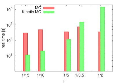
Figure 1: Comparison of real simulation times of standard Monte Carlo and kinetic Monte Carlo. Kinetic MC is highly dependent on the density, which is directly related to the available actions that the system can perform.

III Results

As shown in ref. Pica Ciamarra et al., 2003a, this model is very slow to crystallize. If one prepares the system in the pure crystal state, one can estimate the melting temperature $T_{m}$ through slow heating. The data shown in Fig. 2 for this slow heating gives $T_{m}\simeq 0.15$. In contrast, upon cooling no sign of crystallization is seen and the system remains in a supercooled liquid state until it goes out of equilibrium at a cooling-rate-dependent temperature (Fig. 2). One can extrapolate the specific volume curve of the supercooled liquid branch (dashed line in Fig. 2) and find its intersection with the crystal value. The corresponding temperature, $T_{K}\simeq 0.05$, can be used as an estimate of the Kauzmann temperature Kauzmann (1948).

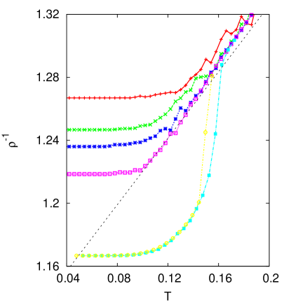
Figure 2: $\rho^{-1}$ as a function of $T$ for different cooling rates. For $\dot{T}=-10^{-5}$ (red) the system goes quickly out of equilibrium, while $\dot{T}=-10^{-6}$ (green), $\dot{T}=-10^{-7}$ (blue) and $\dot{T}=-10^{-8}$ (purple) allow the supercooled metaequilibrium liquid to be found at progressively lower temperatures. Heating from the perfect crystall can be used to estimate $T_{m}$, as in the cyan ($\dot{T}=10^{-8}$) and yellow ($\dot{T}=10^{-9}$) curves.

Relaxation times $\tau_{R}$ can be obtained by means of the self overlap $Q(t,t_{w})$. These times, ploted in Fig. 3, are well fitted with a Vogel-Fulchner-Tamman law

$$\tau_{R}(T)=~{}\tau_{0}~{}\exp[B/(T-T_{0})],$$ (2)

with $T_{0}=0.04$, quite close to $T_{K}$.

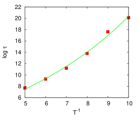
Figure 3: Angell plot showing non-Arrhenius behavior. Full curve is a Vogel-Fulchnet-Tamman fit with $T_{0}=0.04$.

III.1 Metastability limit

We now attempt to establish the lowest temperature at which the supercooled liquid can be equilibrated, i.e. the metastability limit. We have done quenches from the empty lattice to several values of $T_{f}$ (Fig. 4). For $T_{f}\geq 1/8$, the lattice fills up relatively quickly until the density reaches a $T$-dependent plateau after $\sim 10^{3}$–$10^{5}$ steps. The crystal mass fraction $m$ increases more slowly but also reaches a plateau (Fig. 5). The plateau regime is candidate (subject to aging checks, see sec. III.2) for the equilibrium (meta-equilibrium for $T<T_{m}\approx 0.15$) liquid. This being a short-range model, however, the meta-equilibrium state cannot be expected to last forever, and indeed at $T=1/9$ one clearly sees that $\rho$ and $m$ leave the plateau after about $10^{10}$ steps and continue increasing towards the crystal values. We interpret this as a crystal growth regime, where one or more supercritical crystal nucleii have formed and are slowly growing. The system is no longer liquid, but out of equilibrium again.

For $T_{f}=1/12$, however, the behavior is different: the growth of $\rho$ and $m$ is slower, but a plateau is never reached. Instead, both quantities continue to grow towards the crystal values, reaching relatively high values more quickly than systems at higher values of $T_{f}$. The system is never in a metastable state, instead entering a coarsening regime before the metastable liquid can equilibrate. We can thus take $1/12\simeq 0.083$ as a lower bound for $T_{\text{sp}}$. The estimated Kauzmann point, at $T_{K}=0.05$ is thus way past the metastability limit, making it of questionable relevance.

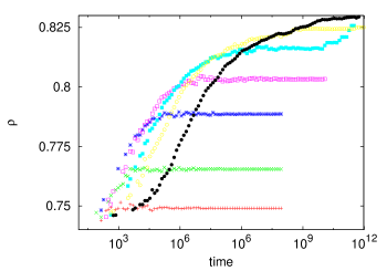
Figure 4: Density vs. time for (from bottom to top) $T=1/5$, 1/6, 1/7, 1/8, 1/9, 1/10, and 1/12.

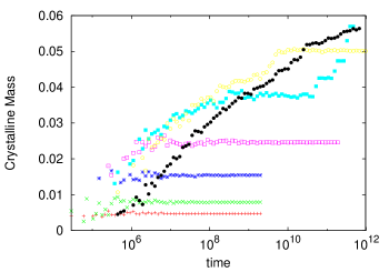
Figure 5: Crystal mass fraction for (from bottom to top) $T=1/5$, 1/6, 1/7, 1/8, 1/9, 1/10, and 1/12.

III.1.1 Short-time dynamics

To locate the thermodynamic spinodal, which serves as a lower bound on the metastability limit, we used the short-time dynamics technique as recently proposed Loscar et al. (2009). The technique is based on the fact that the thermodynamic spinodal is an instability similar to a critical point, but located in the metastable region. Then this instability can be exploited Loscar et al. (2009) to locate the spinodal studying the critical short-time dynamics Janssen et al. (1989); Zheng (2006); Albano et al. (2011). The procedure consists in looking for a power-law time relaxation from an initial state prepared according to some prescription. In equilibrium critical points the power-law regime lasts for a time increasing with the system size, but in the case of spinodals (in a sense metastable critical points) this regime is found only for a finite interval Loscar et al. (2009). The procedure was as follows:

1. Prepare a well equilibrated sample at high temperature $T_{\textsl{i}}=4T_{\textsl{c}}$. This is the disordered initial state.

2. At $t=0$ quench suddenly to $T_{\textsl{f}}\lesssim T_{\textsl{c}}$. Let the system relax while recording the order parameter and its fluctuations up to $t\sim 10^{6}\,$MCS (short time).

3. Look for power-law behavior. The spinodal temperature is determined as that where the power-law regime lasts the longest.

We chose the crystall mass fraction $m(t)$ as order parameter and along with it computed the sample-to-sample fluctuations

$$\chi_{m}(t)=N\sigma_{m}(t)=N\sqrt{\langle[m(t)-\langle m(t)\rangle]^{2}\rangle},$$ (3)

where $\langle\ldots\rangle$ stands for average over thermal history and sample (starting configuration). The normalized fluctuation $\chi_{m}$ should be independent of the system size and invariant under a shift of $m$, avoiding the problem that $m$ is not a proper order parameter for the spinodal point. Thus, in this point we expect a pseudocritical dynamics given by $\chi_{m}(t)\propto t^{\phi}$.

Fig. 6 shows the time evolution of the mass fraction $m$, starting at configurations prepared at $T_{\textsl{i}}=4T_{\textsl{c}}$, for different temperatures (in the supercooled region) and using systems of side $L=21$, and $L=30$. This quantity always increases, being a good parameter to detect the onset of the process of forming the solid phase. Note that size effects disappear for $t>10^{2}$, and also the technique starts to distinguish different temperatures for $t>10^{3}$.

Fig. 7 shows $\chi_{m}(t)$ vs. $t$ for a system of side $L=30$ at different temperatures. These data are obtained with $10^{4}$ runs. We can see a power law behavior in the range $200\leq t\leq 27000$ (more than two decades) at $T=T_{sp}=0.104$. The power law fit gives an exponent $\phi=0.20\pm 0.01$. In the inset of Fig. 7 we plot a comparison of $\chi_{m}(t)$ for a system of $L=21$, showing again that the results are independent of $L$ for $t>200$. From this data we estimate the temperature for the thermodynamic spinodal point as

$$T_{sp}=0.104\pm 0.004.$$ (4)

This temperature is about twice $T_{K}$, confirming our earlier statement that the Kauzmann point is irrelevant in this system.

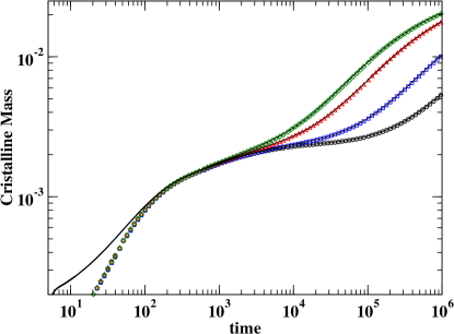
Figure 6: Evolution of the crystal mass fraction starting from the disordered initial condition ($T_{\textsl{i}}=4T_{\textsl{c}}$) with final temperatures $T_{f}=0.08$ (circle), $0.09$ (square), $0.104$ (triangle), and $0.112$ (diamond), and using a system of side $L=21$. Continuous lines are the same temperatures for a bigger system of side $L=30$.

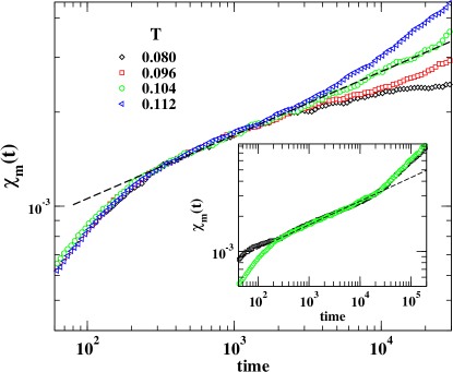
Figure 7: Evolution of the normalized fluctuations for different temperatures (as indicated) for a system of side $L=30$. For $T=T_{sp}=0.104$ we obtain a power law behavior, the dashed black line is a fit of a power law with exponent $\phi=0.203$. The inset shows results for $T=T_{sp}$ and two system sides $L=21$ (black squares) and $L=30$ (green circles).

III.2 Aging

To study aging, we consider the self overlap $Q(t,t_{w})$ as a function of two times for waiting times $t_{w}\geq 10^{6}$, starting with the lattice empty, in the region of slow approach to the plateau of the density (Fig. 4).

For $T>1/8$ we find that time-traslation invariance (TTI) holds, i.e. $Q(t,t_{w})\equiv Q(t-t_{w})$ and consequently no ageing is observed (not shown). On the other hand, for $1/T=9$, we find $t_{w}$ dependence (Fig. 8). The system shows signs of aging from $t_{w}=10^{6}$ to $t_{w}\sim 10^{8}$; after that the curves start becoming close to each other. This interruption of ageing coincides roughly with the appearence of the plateau in $\rho$ and $m$ (Figs. 4 and 5), and is an indication that the liquid is equilibrating. This plateau lasts up to $t\sim 10^{11}$, when the system leaves equilibrium again to begin crystallizing.

In the aging regime, structural glasses have been found to obey the scaling

$$Q(t,t_{w})=f\left(\frac{t}{t_{w}^{\nu}}\right),$$ (5)

with $\nu$ close to 1 Struik (1977); Grigera et al. (2004). This relation clearly cannot apply to the data of Fig. 8 across all waiting times, it is because the curves coincide for $t>3\times 10^{9}$. We can however compute an effective scaling exponent $\nu(t_{w})$ Struik (1977); Warren and Rottler (2013): Defining a characteristic decay time $t_{c}$ using a fixed thershold for the overlap (we chose $Q(t_{c})=0.3$), one can define an effective scaling exponent through $\nu_{\text{eff}}(t_{w})=\partial\ln t_{c}/\partial\ln t_{w}$. Rather than evaluating the derivative numerically, we use a sigmoidal fit for $t_{c}$ vs $t_{w}$ Warren and Rottler (2013); see Fig. 9. The low values of $\nu$ for $t_{w}=10^{8}$ confirm that the liquid is reaching (meta)equilibrium. However, $\nu$ is never higher than 0.5, quite far from the value $\nu\approx 1$. According to ref. Warren and Rottler (2013), and taking also into account the behavior of the density, we interpret this as evidence that the model is always “too close” to equilibrium to reproduce the experimental aging behavior. In other words, the dynamics is starting to become slow, so that it takes a relatively long time for the system to equilibrate, but there is no proper aging regime; equilibrium is reached relatively soon after one-time quantities begin to stabilize (while experimentally aging in the correlation function happens with very little variation of one-time quantities Struik (1977). The situation is similar at the other temperatures we have studied (above and near the metastability limit), see Table 1.

$T$	$\nu_{\text{max}}$
1/8	0.441
1/9	0.476
1/10	0.455

Table 1: Estimate of maximum value of the aging exponent $\nu$ for different temperatures

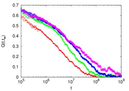
Figure 8: Overlap vs. time at $T=1/9$ for $t_{w}=10^{6}$ (red), $t_{w}=10^{7}$ (green) $t_{w}=2\times 10^{8}$ (blue) and $t_{w}=2\times 10^{9}$ (purple).

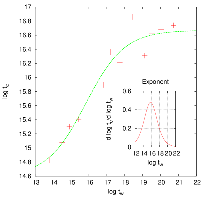
Figure 9: Characteristic time of the relaxation ($t_{c}$) vs. $t_{w}$ for $T=1/9$. The full line is a fit to a 4 parameter sigmoid $S(t)=A+\frac{B}{1+e^{-(t/D-C)}}$. Inset: effective exponent $\nu_{\text{eff}}=\partial\ln t_{c}/\partial\ln t_{w}$.

Of course, at lower temperatures the dynamics will be slower, and it will take longer to reach equilibrium. However, as shown above temperatures beyond $0.10$ are below the metastability limit, so that the out-of-equilibrium behavior in that region corresponds to a coarsening regime, where aging is qualitatively different from a structural glass Corberi et al. (2011).

IV Conclusions

We have revisited the Pica Ciamarra-Tarzia-de Candia-Coniglio lattice glass. While it reproduces many features of supercooled liquids, as previously pointed out, the present analysis shows that it is not suitable to study the deeply supercooled regime. We have shown that the metastability limit is at a temperature not too far from the melting point, making the metastable liquid nonexistant for $T\lesssim 0.10$, above the estimated Kauzmann temperature. Although thermodynamic studies, and in particular theories relating dynamic behavior to thermodynamic properties are not invalidated by an unreachable Kauzmann point (as long as the metastable liquid exists), in the present model the range of validity of such studies seems to be too restricted.

Studies of the structural glass (out of equilibrium) state are also somewhat limited. Beyond the metastability limit, the out of equilibrium behavior is that of coarsening, in principle rather different than what has been observed in experimental and numerical studies of structural glasses. The range between $T=0.10$ and melting indeed corresponds to the structural glass situation, i.e. an out-of-equilibrium system slowly evolving towards an equilibrium liquid. However, we have found that the $t/t_{w}$ scaling is not obeyed by this model, probably because it reaches equilibrium too quickly in this temperature range. When cooled further, relaxation becomes slower and one would hope to get something closer to a structural glass; unfortunately the liquid ceases to exist before a regime with the correct scaling sets in.