On the Inductive Bias of Dropout

Abstract

Dropout is a simple but effective technique for learning in neural networks and other settings. A sound theoretical understanding of dropout is needed to determine when dropout should be applied and how to use it most effectively. In this paper we continue the exploration of dropout as a regularizer pioneered by Wager, et.al. We focus on linear classification where a convex proxy to the misclassification loss (i.e. the logistic loss used in logistic regression) is minimized. We show:

• when the dropout-regularized criterion has a unique minimizer,

• when the dropout-regularization penalty goes to infinity with the weights, and when it remains bounded,

• that the dropout regularization can be non-monotonic as individual weights increase from 0, and

• that the dropout regularization penalty may not be convex.

This last point is particularly surprising because the combination of dropout regularization with any convex loss proxy is always a convex function.

In order to contrast dropout regularization with $L_{2}$ regularization, we formalize the notion of when different sources are more compatible with different regularizers. We then exhibit distributions that are provably more compatible with dropout regularization than $L_{2}$ regularization, and vice versa. These sources provide additional insight into how the inductive biases of dropout and $L_{2}$ regularization differ. We provide some similar results for $L_{1}$ regularization.

1 Introduction

Since its prominent role in a win of the ImageNet Large Scale Visual Recognition Challenge (Hinton, 2012; Hinton et al., 2012), there has been intense interest in dropout (see the work by Dahl (2012); L. Deng (2013); Dahl et al. (2013); Wan et al. (2013); Wager et al. (2013); Baldi and Sadowski (2013); Van Erven et al. (2014)). This paper studies the inductive bias of dropout: when one chooses to train with dropout, what prior preference over models results? We show that dropout training shapes the learner’s search space in a much different way than $L_{1}$ or $L_{2}$ regularization. Our results shed new insight into why dropout prefers rare features, how the dropout probability affects the strength of regularization, and how dropout restricts the co-adaptation of weights.

Our theoretical study will concern learning a linear classifier via convex optimization. The learner wishes to find a parameter vector ${\bf w}$ so that, for a random feature-label pair $({\bf x},y)\in{\bf R}^{n}\times\{-1,1\}$ drawn from some joint distribution $P$, the probability that $\mathrm{sign}({\bf w}\cdot{\bf x})\neq y$ is small. It does this by using training data to try to minimize ${\bf E}(\ell(y{\bf w}\cdot{\bf x}))$, where $\ell(z)=\ln(1+\exp(-z))$ is the loss function associated with logistic regression.

We have chosen to focus on this problem for several reasons. First, the inductive bias of dropout is not well understood even in this simple setting. Second, linear classifiers remain a popular choice for practical problems, especially in the case of very high-dimensional data. Third, we view a thorough understanding of dropout in this setting as a mandatory prerequisite to understanding the inductive bias of dropout when applied in a deep learning architecture. This is especially true when the preference over deep learning models is decomposed into preferences at each node. In any case, the setting that we are studying faithfully describes the inductive bias of a deep learning system at its output nodes.

We will borrow the following clean and illuminating description of dropout as artificial noise due to Wager et al. (2013). An algorithm for linear classification using loss $\ell$ and dropout updates its parameter vector ${\bf w}$ online, using stochastic gradient descent. Given an example $({\bf x},y)$, the dropout algorithm independently perturbs each feature $i$ of ${\bf x}$: with probability $q$, $x_{i}$ is replaced with $0$, and, with probability $p=1-q$, $x_{i}$ is replaced with $x_{i}/p$. Equivalently, ${\bf x}$ is replaced by ${\bf x}+{\boldsymbol{\nu}}$, where

$$\nu_{i}=\left\{\begin{array}[]{ll}-x_{i}&\mbox{with probability $q$}\\ (1/p-1)x_{i}&\mbox{with probability $p=1-q$}\end{array}\right.$$

before performing the stochastic gradient update step. (Note that, while ${\boldsymbol{\nu}}$ obviously depends on ${\bf x}$, if we sample the components of ${\bf b}\in\{-1,1/p-1\}^{n}$ independently of one another and ${\bf x}$, by choosing $b_{i}=-1$ with the dropout probability $q$, then we may write $\nu_{i}=b_{i}x_{i}$.)

Stochastic gradient descent is known to converge under a broad variety of conditions (Kushner and Yin, 1997). Thus, if we abstract away sampling issues as done by Breiman (2004); Zhang (2004); Bartlett et al. (2006); Long and Servedio (2010), we are led to consider

$${\bf w}^{*}\stackrel{{\scriptstyle\textup{def}}}{{=}}\mathrm{argmin}_{{\bf w}}{\bf E}_{({\bf x},y)\sim P,{\boldsymbol{\nu}}}(\ell(y{\bf w}\cdot({\bf x}+{\boldsymbol{\nu}})))$$

as dropout can be viewed as a stochastic gradient update of this global objective function. We call this objective the dropout criterion, and it can be viewed as a risk on the dropout-induced distribution. (Abstracting away sampling issues is consistent with our goal of concentrating on the inductive bias of the algorithm. From the point of view of a bias-variance decomposition, we do not intend to focus on the large-sample-size case, where the variance is small, but rather to focus on the contribution from the bias where $P$ could be an empirical sample distribution. )

We start with the observation of Wager et al. (2013) that the dropout criterion may be decomposed as

$${\bf E}_{({\bf x},y)\sim P,{\boldsymbol{\nu}}}(\ell(y{\bf w}\cdot({\bf x}+{\boldsymbol{\nu}})))={\bf E}_{({\bf x},y)\sim P}(\ell(y{\bf w}\cdot{\bf x}))+\mathrm{reg}_{D,q}({\bf w}),$$ (1)

where $\mathrm{reg}_{D,q}$ is non-negative, and depends only on the marginal distribution $D$ over the feature vectors ${\bf x}$ (along with the dropout probability $q$), and not on the labels. This leads naturally to a view of dropout as a regularizer.

A popular style of learning algorithm minimizes an objective function like the RHS of (1), but where $\mathrm{reg}_{D,q}({\bf w})$ is replaced by a norm of ${\bf w}$. One motivation for algorithms in this family is to first replace the training error with a convex proxy to make optimization tractable, and then to regularize using a convex penalty such as a norm, so that the objective function remains convex.

We show that $\mathrm{reg}_{D,q}({\bf w})$ formalizes a preference for classifiers that assign a very large weight to a single feature. This preference is stronger than what one gets from a penalty proportional to $||{\bf w}||_{1}$. In fact, we show that, despite the convexity of the dropout risk, $\mathrm{reg}_{D,q}$ is not convex, so that dropout provides a way to realize the inductive bias arising from a non-convex penalty, while still enjoying the benefit of convexity in the overall objective function (see the plots in Figures 1, 2 and 3). Figure 1 shows the even more surprising result that the dropout regularization penalty is not even monotonic in the absolute values of the individual weights.

It is not hard to see that $\mathrm{reg}_{D,q}({\bf 0})=0$. Thus, if $\mathrm{reg}_{D,q}({\bf w})$ is greater than the expected loss incurred by ${\bf 0}$ (which is $\ln 2$), then it might as well be infinity, because dropout will prefer ${\bf 0}$ to ${\bf w}$. However, in some cases, dropout never reaches this extreme – it remains willing to use a model, even if its parameter is very large, unlike methods that use a convex penalty. In particular,

$$\mathrm{reg}_{D,q}(w_{1},0,0,0,...,0)<\ln 2$$

for all $D$, no matter how large $w_{1}$ gets; of course, the same is true for the other features. On the other hand, except for some special cases (which are detailed in the body of the paper),

$$\mathrm{reg}_{D,q}(cw_{1},cw_{2},0,0,...,0)$$

goes to infinity with $c$. It follows that $\mathrm{reg}_{D,q}$ cannot be approximated to within any factor, constant or otherwise, by a convex function of ${\bf w}$.

To get a sense of which sources dropout can be successfully applied to, we compare dropout with an algorithm that regularizes using $L_{2}$, by minimizing the $L_{2}$ criterion:

$${\bf E}_{({\bf x},y)\sim P}(\ell(y{\bf w}\cdot{\bf x}))+\frac{\lambda}{2}||{\bf w}||_{2}^{2}.$$ (2)

Will will use “$L_{2}$” as a shorthand to refer to an algorithm that minimizes (2). Note that $q$, the probability of dropping out an input feature, plays a role in dropout analogous to $\lambda$. In particular, as $q$ goes to zero the examples remain unperturbed and the dropout regularization has no effect.

Informally, we say that joint probability distributions $P$ and $Q$ separate dropout from $L_{2}$ if, when the same parameters $\lambda$ and $q$ are used for both $P$ and $Q$, then using dropout leads to a much more accurate hypothesis for $P$, and using $L_{2}$ leads to a much more accurate hypothesis for $Q$. This enables us to illustrate the inductive biases of the algorithms through the use of contrasting sources that either align or are incompatible with the algorithms’ inductive bias. Comparing with another regularizer helps to restrict these illustrative examples to “reasonable” sources, which can be handled using another regularizer. Ensuring that the same values of the regularization parameter are used for both $P$ and $Q$ controls for the amount of regularization, and ensures that the difference is due to the model preferences of the respective regularizers. This style of analysis is new, as far as we know, and may be a useful tool for studying the inductive biases of other algorithms and in other settings.

Related previous work. Our research builds on the work of Wager et al. (2013), who analyzed dropout for random $(x,y)$ pairs where the distribution of $y$ given $x$ comes from a member of the exponential family, and the quality of a model is evaluated using the log-loss. They pointed out that, in these cases, the dropout criterion can be decomposed into the original loss and a term that does not depend on $y$, which therefore can be viewed as a regularizer. They then proposed an approximation to this dropout regularizer, discussed its relationship with other regularizers and training algorithms, and evaluated it experimentally. Baldi and Sadowski (2013) exposed properties of dropout when viewed as an ensemble method (see also Bachman et al. (2014)). Van Erven et al. (2014) showed that applying dropout for online learning in the experts setting leads to algorithms that adapt to important properties of the input without requiring doubling or other parameter-tuning techniques, and Abernethy et al. (2014) analyzed a class of methods including dropout by viewing these methods as smoothers. The impact of dropout on generalization (roughly, how much dropout restricts the search space of the learner, or, from a bias-variance point of view, its impact on variance) was studied by Wan et al. (2013) and Wager et al. (2014). The latter paper considers a variant of dropout compatible with a poisson source, and shows that under some assumptions this dropout variant converges more quickly to its infinite sample limit than non-dropout training, and that the Bayes-optimal predictions are preserved under the modified dropout distribution. Our results complement theirs by focusing on the effect of the original dropout on the algorithm’s bias.

Section 2 defines our notation and characterizes when the dropout criterion has a unique minimizer. Section 3 presents many additional properties of the dropout regularizer. Section 4 formally defines when two distributions separate two algorithms or regularizers. Sections 5 and 6 give sources over ${\bf R}^{2}$ that separate dropout and $L_{2}$. Section 7 provides plots demonstrating that the same distributions separated dropout from $L_{1}$ regularization. Sections 8 and 9 give separation results from $L_{2}$ with many features.

2 Preliminaries

We use ${\bf w}^{*}$ for the optimizer of the dropout criterion, $q$ for the probability that a feature is dropped out, and $p=1-q$ for the probability that a feature is kept throughout the paper. As in the introduction, if $X\subseteq{\bf R}^{n}$ and $P$ is a joint distribution over $X\times\{-1,1\}$, define

$${\bf w}^{*}(P,q)\stackrel{{\scriptstyle\textup{def}}}{{=}}\mathrm{argmin}_{{\bf w}}{\bf E}_{({\bf x},y)\sim P,{\boldsymbol{\nu}}}(\ell(y{\bf w}\cdot({\bf x}+{\boldsymbol{\nu}})))$$ (3)

where $\nu_{i}=b_{i}x_{i}$ for $b_{1},...,b_{n}$ sampled independently at random from $\{-1,1/p-1\}$ with ${\bf Pr}(b_{i}=1/p-1)=p=1-q$, and $\ell(z)$ is the logistic loss function:

$$\ell(z)=\ln(1+\exp(-z)).$$

For some analyses, an alternative representation of ${\bf w}^{*}(P,q)$ will be easier to work with. Let $r_{1},...,r_{n}$ be sampled randomly from $\{0,1\}$, independently of $({\bf x},y)$ and one another, with ${\bf Pr}(r_{i}=1)=p$. Defining ${\bf r}\odot{\bf x}=(x_{1}r_{1},...,x_{n}r_{n})$, we have the equivalent definition

$${\bf w}^{*}(P,q)=p\;\mathrm{argmin}_{{\bf w}}{\bf E}_{({\bf x},y)\sim P,{\bf r}}(\ell(y{\bf w}\cdot({\bf r}\odot{\bf x}))).$$ (4)

To see that they are equivalent, note that

$${\bf E}(\ell(y{\bf w}\cdot({\bf x}+{\boldsymbol{\nu}}))) ={\bf E}\left(\ell\left(y{\bf w}\cdot\left(\frac{{\bf r}\odot{\bf x}}{p}\right)\right)\right)$$

$$={\bf E}(\ell(y({\bf w}/p)\cdot({\bf r}\odot{\bf x}))).$$

Although this paper focuses on the logistic loss, the above definitions can be used for any loss function $\ell()$. Since the dropout criterion is an expectation of $\ell()$, we have the following obvious consequence.

Proposition 1

If loss $\ell(\cdot)$ is convex, then the dropout criterion is also a convex function of ${\bf w}$.

Similarly, we use ${\bf v}$ for the optimizer of the $L_{2}$ regularized criterion:

$${\bf v}(P,\lambda)\stackrel{{\scriptstyle\textup{def}}}{{=}}\mathrm{argmin}_{{\bf w}}{\bf E}_{({\bf x},y)\sim P}(\ell(y{\bf w}\cdot{\bf x}))+\frac{\lambda}{2}||{\bf w}||^{2}.$$ (5)

It is not hard to see that the $\frac{\lambda}{2}||{\bf w}||^{2}$ term implies that ${\bf v}(P,\lambda)$ is always well-defined. On the other hand, ${\bf w}^{*}(P,q)$ is not always well-defined, as can be seen by considering any distribution concentrated on a single example. This motivates the following definition.

Definition 2

Let $P$ be a joint distribution with support contained in ${\bf R}^{n}\times\{-1,1\}$. A feature $i$ is perfect modulo ties for $P$ if either $yx_{i}\geq 0$ for all ${\bf x}$ in the support of $P$, or $yx_{i}\leq 0$ for all ${\bf x}$ in the support of $P$.

Put another way, $i$ is perfect modulo ties if there is a linear classifier that only pays attention to feature $i$ and is perfect on the part of $P$ where $x_{i}$ is nonzero.

Proposition 3

For all finite domains $X\subseteq{\bf R}^{n}$, all distributions $P$ with support in $X$, and all $q\in(0,1)$, we have that ${\bf E}_{({\bf x},y)\sim P,{\bf r}}(\ell(y{\bf w}\cdot({\bf r}\odot{\bf x})))$ has a unique minimum in ${\bf R}^{n}$ if and only if no feature is perfect modulo ties for $P$.

Proof: Assume for contradiction that feature $i$ is perfect modulo ties for $P$ and some ${\bf w}^{\circledast}$ is the unique minimizer of ${\bf E}_{({\bf x},y)\sim P,{\bf r}}(\ell(y{\bf w}\cdot({\bf r}\odot{\bf x})))$. Assume w.l.o.g. that $yx_{i}\geq 0$ for all ${\bf x}$ in the support of $P$ (the case where $yx_{i}\leq 0$ is analogous). Increasing $w^{\circledast}_{i}$ keeps the loss unchanged on examples where $x_{i}=0$ and decreases the loss on the other examples in the support of $P$, contradicting the assumption that ${\bf w}^{\circledast}$ was a unique minimizer of the expected loss.

Now, suppose then each feature $i$ has both examples where $yx_{i}>0$ and examples where $yx_{i}<0$ in the support of $P$. Since the support of $P$ is finite, there is a positive lower bound on the probability of any example in the support. With probability $p(1-p)^{n-1}$, component $r_{i}$ of random vector ${\bf r}$ is non-zero and the remaining $n-1$ components are all zero. Therefore as $w_{i}$ increases without bound in the positive or negative direction, ${\bf E}_{({\bf x},y)\sim P,{\bf r}}(\ell(y{\bf w}\cdot({\bf r}\odot{\bf x})))$ also increases without bound. Since ${\bf E}_{({\bf x},y)\sim P,{\bf r}}(\ell(y{\bf 0}\cdot({\bf r}\odot{\bf x})))=\ln 2$, there is a value $M$ depending only on distribution $P$ and the dropout probability such that minimizing ${\bf E}_{({\bf x},y)\sim P,{\bf r}}(\ell(y{\bf w}\cdot({\bf r}\odot{\bf x})))$ over ${\bf w}\in[-M,M]^{n}$ is equivalent to minimizing ${\bf E}_{({\bf x},y)\sim P,{\bf r}}(\ell(y{\bf w}\cdot({\bf r}\odot{\bf x})))$ over ${\bf R}^{n}$. Since ${\bf Pr}_{({\bf x},y)}(x_{i}=0)\neq 1$ for all $i$, $\{{\bf r}\odot{\bf x}:{\bf r}\in\{0,1\}^{n},{\bf x}\in X\}$ has full rank and therefore ${\bf E}_{({\bf x},y)\sim P,{\bf r}}(\ell(y{\bf w}\cdot({\bf r}\odot{\bf x})))$ is strictly convex. Since a strictly convex function defined on a compact set has a unique minimum, ${\bf E}_{({\bf x},y)\sim P,{\bf r}}(\ell(y{\bf w}\cdot({\bf r}\odot{\bf x})))$ has a unique minimum on $[-M,M]^{n}$, and therefore on ${\bf R}^{n}$.  

See Table 1 for a summary of the notation used in the paper.

${\bf x}=(x_{1},\ldots,x_{n})$ feature vector in ${\bf R}^{n}$ $y$ label in $\{-1,+1\}$ ${\bf w}=(w_{1},\ldots,w_{n})$ weight vector in ${\bf R}^{n}$ $\ell(y{\bf w}\cdot{\bf x})$ loss function, generally the logistic loss: $\ln(1+\exp(-y{\bf w}\cdot{\bf x}))$ $P$, $Q$ source distributions over $({\bf x},y)$ pairs, varies by section $D$ marginal distribution over ${\bf x}$ $q$ feature dropout probability in $(0,1)$ $p=1-q$ probability of keeping a feature $\lambda$ $L_{2}$ regularization parameter ${\boldsymbol{\nu}}=(\nu_{1},\ldots,\nu_{n})$ additive dropout noise, $\nu_{i}\in\{-x_{i},x_{i}/p-x_{i}\}$ ${\bf r}=(r_{1},\ldots,r_{n})$ multiplicative dropout noise, $r_{i}\in\{0,1\}$ $\odot$ component-wise product: ${\bf r}\odot{\bf x}=(r_{1}x_{1},\ldots,r_{n}x_{n})$ ${\bf w}^{*}(P,q)$ and ${\bf w}^{*}$ minimizer of dropout criterion: ${\bf E}(\ell(y\;{\bf w}\cdot({\bf x}+{\boldsymbol{\nu}})))$ ${\bf w}^{\circledast}={\bf w}^{*}/p$ minimizer of expected loss ${\bf E}(\ell(y\;{\bf w}\cdot({\bf r}\odot{\bf x})))$ ${\bf v}(P,\lambda)$ and ${\bf v}$ minimizer of $L_{2}$-regularized loss $\mathrm{reg}_{D,q}({\bf w})$ regularization due to dropout $J$, $K$ criteria to be optimized, varies by sub-section $g({\bf w})$, ${\bf g}$ gradients of the current criterion $\mathrm{er}_{P}({\bf w})$ 0-1 classification generalization error of $\mathrm{sign}({\bf w}\cdot x)$

Table 1: Summary of notation used throughout the paper.

3 Properties of the Dropout Regularizer

We start by rederiving the regularization function corresponding to dropout training previously presented in Wager et al. (2013), specialized to our context and using our notation. The first step is to write $\ell(y{\bf w}\cdot{\bf x})$ in an alternative way that exposes some symmetries:

$$\ell(y{\bf w}\cdot{\bf x}) =\ln(1+\exp(-y{\bf w}\cdot{\bf x}))$$

$$=\ln\left(\frac{\exp(y({\bf w}\cdot{\bf x})/2)+\exp(-y({\bf w}\cdot{\bf x})/2)}{\exp(y({\bf w}\cdot{\bf x})/2)}\right)$$

$$=\ln\left(\frac{\exp(({\bf w}\cdot{\bf x})/2)+\exp(-({\bf w}\cdot{\bf x})/2)}{\exp(y({\bf w}\cdot{\bf x})/2)}\right).$$ (6)

This then implies

$$\mathrm{reg}_{D,q}({\bf w}) ={\bf E}(\ell(y{\bf w}\cdot({\bf x}+{\boldsymbol{\nu}})))-{\bf E}(\ell(y{\bf w}\cdot{\bf x}))$$

$$={\bf E}\left(\ln\left(\frac{\exp(({\bf w}\cdot({\bf x}+{\boldsymbol{\nu}}))/2)+\exp(-({\bf w}\cdot({\bf x}+{\boldsymbol{\nu}}))/2)}{\exp(y({\bf w}\cdot({\bf x}+{\boldsymbol{\nu}}))/2)}\times\frac{\exp(y({\bf w}\cdot{\bf x})/2)}{\exp(({\bf w}\cdot{\bf x})/2)+\exp(-({\bf w}\cdot{\bf x})/2)}\right)\right)$$

$$={\bf E}\Big{(}\ln\left(\frac{\exp(({\bf w}\cdot({\bf x}\!+\!{\boldsymbol{\nu}}))/2)\!+\!\exp(-({\bf w}\cdot({\bf x}\!+\!{\boldsymbol{\nu}}))/2)}{\exp(({\bf w}\cdot{\bf x})/2)\!+\!\exp(-({\bf w}\cdot{\bf x})/2)}\right)-y({\bf w}\cdot{\boldsymbol{\nu}})/2\Big{)}.$$

Since ${\bf E}({\boldsymbol{\nu}})={\bf 0}$, we get the following.

Proposition 4

(Wager et al., 2013)

$$\mathrm{reg}_{D,q}({\bf w})={\bf E}\left(\ln\left(\frac{\exp({\bf w}\cdot({\bf x}+{\boldsymbol{\nu}})/2)+\exp(-{\bf w}\cdot({\bf x}+{\boldsymbol{\nu}})/2)}{\exp(({\bf w}\cdot{\bf x})/2)+\exp(-({\bf w}\cdot{\bf x})/2)}\right)\right).$$ (7)

Using a Taylor expansion, Wager et al. (2013) arrived at the following approximation:

$$\frac{q}{2(1-q)}\sum_{i}w_{i}^{2}{\bf E}_{{\bf x}}\left(\frac{x_{i}^{2}}{(1+\exp(-\frac{{\bf w}\cdot{\bf x}}{2}))(1+\exp(\frac{{\bf w}\cdot{\bf x}}{2})}\right).$$ (8)

This approximation suggests two properties: the strength of the regularization penalty decreases exponentially in the prediction confidence $|{\bf w}\cdot{\bf x}|$, and that the regularization penalty goes to infinity as the dropout probability $q$ goes to 1. However, ${\bf w}\cdot{\boldsymbol{\nu}}$ can be quite large, making a second-order Taylor expansion inaccurate. In fact, the analysis in this section suggests that the regularization penalty does not decrease with the confidence and that the regularization penalty increases linearly with $q=1-p$ (Figure 1, Theorem 8, Proposition 9).

The following propositions show that $\mathrm{reg}_{D,q}({\bf w})$ satisfies at least some of the intuitive properties of a regularizer.

Proposition 5

$\mathrm{reg}_{D,q}({\boldsymbol{0}})=0$.

Proposition 6

(Wager et al., 2013) The contribution of each ${\bf x}$ to the regularization penalty (7) is non-negative: for all ${\bf x}$,

$${\bf E}_{{\boldsymbol{\nu}}}\left(\ln\left(\frac{\exp(({\bf w}\cdot({\bf x}+{\boldsymbol{\nu}}))/2)+\exp(-({\bf w}\cdot({\bf x}+{\boldsymbol{\nu}}))/2)}{\exp(({\bf w}\cdot{\bf x})/2)+\exp(-({\bf w}\cdot{\bf x})/2)}\right)\right)\geq 0.$$

Proof: The proposition follows from Jensen’s Inequality.  

The ${\bf w}^{*}(P,q)$ vector learned by dropout training minimizes ${\bf E}_{({\bf x},y)\sim P}(\ell(y{\bf w}\cdot{\bf x}))+\mathrm{reg}_{D,q}({\bf w})$. However, the ${\boldsymbol{0}}$ vector has $\ell(y{\boldsymbol{0}}\cdot{\bf x})=\ln(2)$ and $\mathrm{reg}_{D,q}({\boldsymbol{0}})=0$, implying:

Proposition 7

$\mathrm{reg}_{D,q}({\bf w}^{*})\leq\ln(2)$.

Thus any regularization penalty greater than $\ln(2)$ is effectively equivalent to a regularization penalty of $\infty$.

We now present new results based on analyzing the exact $\mathrm{reg}_{D,q}({\bf w})$. The next properties show that the dropout regularizer is emphatically not like other convex or norm-based regularization penalties in that the dropout regularization penalty always remains bounded when a single component of the weight vector goes to infinity (see also Figure 1).

Theorem 8

For all dropout probabilities $1-p\in(0,1)$, all $n$, all marginal distributions $D$ over $n$-feature vectors, and all indices $1\leq i\leq n$,

$$\sup_{w_{i}}\mathrm{reg}_{D,q}(\underbrace{0,\ldots,0}_{i-1},w_{i},\underbrace{0,\ldots,0}_{n-i})\leq{\bf Pr}_{D}(x_{i}\neq 0)(1-p)\ln(2)\;<\;\ln 2.$$

Proof: Fix arbitrary $n$, $p$, $i$, and $D$. We have

$$\mathrm{reg}_{D,q}(\underbrace{0,\ldots,0}_{i-1},w_{i},\underbrace{0,\ldots,0}_{n-i})$$

$$={\bf E}_{{\bf x},{\boldsymbol{\nu}}}\left(\ln\left(\frac{\exp(-w_{i}(x_{i}\!+\!\nu_{i})/2)\!+\!\exp(w_{i}(x_{i}\!+\!\nu_{i})/2)}{\exp(-w_{i}x_{i}/2)\!+\!\exp(w_{i}x_{i}/2)}\right)\right).$$

Fix an arbitrary ${\bf x}$ in the support of $D$ and examine the expectation over ${\boldsymbol{\nu}}$ for that ${\bf x}$. Recall that $x_{i}+\nu_{i}$ is 0 with probability $1-p$ and is $x_{i}/p$ with probability $p$, and we will use the substitution $z=|w_{i}x_{i}|/2$.

$${\bf E}_{{\boldsymbol{\nu}}} \left(\ln\left(\frac{\exp(\frac{-w_{i}(x_{i}+\nu_{i})}{2})+\exp(\frac{w_{i}(x_{i}+\nu_{i})}{2})}{\exp(\frac{-w_{i}x_{i}}{2})+\exp(\frac{w_{i}x_{i}}{2})}\right)\right)$$ (9)

$$=(1-p)\ln(2)+p\ln\left(\exp(\frac{z}{p})+\exp(\frac{-z}{p})\right)-\ln\left(\exp(z)+\exp(-z)\right).$$ (10)

We now consider cases based on whether or not $z$ is 0. When $z=0$ (so either $w_{i}$ or $x_{i}$ is $0$) then (10) is also 0.

If $z\neq 0$ then consider the derivative of (10) w.r.t. $z$, which is

$$\frac{\exp(z/p)-\exp(-z/p)}{\exp(z/p)+\exp(-z/p)}-\frac{\exp(z)-\exp(-z)}{\exp(z)+\exp(-z)}.$$

This derivative is positive since $z>0$ and $0<p<1$. Therefore (10) is bounded by its limit as $z\rightarrow\infty$, which is $(1-p)\ln(2)$, in this case.

Since (9) is 0 when $x_{i}=0$ and is bounded by $(1-p)\ln(2)$ otherwise, the expectation over ${\bf x}$ of (9) is bounded ${\bf Pr}_{D}(x_{i}\neq 0)(1-p)\ln(2)$, completing the proof.  

Since line (10) is derived using a chain of equalities, the same proof ideas can be used to show that Theorem 8 is tight.

Proposition 9

Under the conditions of Theorem 8,

$$\lim_{w_{i}\rightarrow\infty}\mathrm{reg}_{D,q}(\underbrace{0,\ldots,0}_{i-1},w_{i},\underbrace{0,\ldots,0}_{n-i})={\bf Pr}_{D}(x_{i}\neq 0)(1-p)\ln(2).$$

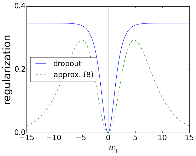
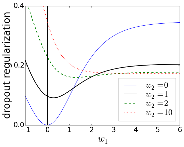
Figure 1: The $p=1/2$ dropout regularization for ${\bf x}=(1,1)$ as a function of $w_{i}$ when the other weights are 0 together with its approximation (8) (left) and as a function of $w_{1}$ for different values of the second weight (right).

Note that this bound on the regularization penalty depends neither on the range nor expectation of $x_{i}$. In particular, it has a far different character than the approximation of Equation (8).

In Theorem 8 the other weights are fixed at 0 as $w_{i}$ goes to infinity. An additional assumption implies that the regularization penalty remains bounded even when the other components are non-zero. Let ${\bf w}$ be a weight vector such that for all ${\bf x}$ in the support of $D$ and dropout noise vectors ${\boldsymbol{\nu}}$ we have $|\sum_{j\neq i}w_{j}(x_{j}+\nu_{j})|\leq M$ for some bound $M$ (this implies that $|\sum_{j\neq i}w_{j}x_{j}|\leq M$ also). Then

$$\mathrm{reg}_{D,q}({\bf w}) ={\bf E}_{{\bf x},{\boldsymbol{\nu}}}\left(\left(\frac{\exp(\frac{{\bf w}\cdot({\bf x}\!+\!{\boldsymbol{\nu}})}{2})\!+\!\exp(-\frac{{\bf w}\cdot({\bf x}\!+\!{\boldsymbol{\nu}})}{2})}{\exp(\frac{{\bf w}\cdot{\bf x}}{2})\!+\!\exp(-\frac{{\bf w}\cdot{\bf x}}{2})}\right)\right)$$

$$\leq{\bf E}_{x_{i},\nu_{i}}\left(\log\left(\frac{\exp(\frac{M-w_{i}(x_{i}\!+\!\nu_{i})}{2}\!+\!\exp(\frac{M+w_{i}(x_{i}\!+\!\nu_{i})}{2})}{\exp(-\frac{M-w_{i}x_{i}}{2}\!+\!\exp(-\frac{M+w_{i}x_{i}}{2})}\right)\right)$$

$$\leq M\!+\!{\bf E}_{x_{i},\nu_{i}}\left(\log\left(\frac{\exp(-\frac{w_{i}x_{i}\!+\!\nu_{i}}{2})\!+\!\exp(\frac{w_{i}(x_{i}\!+\!\nu_{i})}{2})}{\exp(\frac{-w_{i}x_{i}}{2})\!+\!\exp(\frac{w_{i}x_{i}}{2})}\right)\right).$$ (11)

Using (11) instead of the first line in Theorem 8’s proof gives the following.

Proposition 10

Under the conditions of Theorem 8, if the weight vector ${\bf w}$ has the property that $|\sum_{j\neq i}w_{j}(x_{j}+\nu_{j})|\leq M$ for each ${\bf x}$ in the support of $D$ and all of its corresponding dropout noise vectors ${\boldsymbol{\nu}}$ then

$$\sup_{\omega}\mathrm{reg}_{D,q}(w_{1},w_{2},\ldots,w_{i-1},\omega,w_{i+1},\ldots,w_{n})\leq M+{\bf Pr}_{D}(x_{i}\neq 0)(1-p)\ln(2).$$

Proposition 10 shows that the regularization penalty starting from a non-zero initial weight vector remains bounded as any one of its components goes to infinity. On the other hand, unless $M$ is small, the bound will be larger than the dropout criterion for the zero vector. This is a natural consequence as the starting weight vector ${\bf w}$ could already have a large regularization penalty.

The derivative of (10) in the proof of Theorem 8 implies that the dropout regularization penalty is monotonic in $|w_{i}|$ when the other weights are zero. Surprisingly, this is does not hold in general. The dropout regularization penalty due to a single example (as in Proposition 6) can be written as

$${\bf E}_{{\boldsymbol{\nu}}}\left(\ln\left(\textstyle\exp(\frac{{\bf w}\cdot({\bf x}+{\boldsymbol{\nu}})}{2})+\exp(\frac{-{\bf w}\cdot({\bf x}+{\boldsymbol{\nu}})}{2})\right)\right)-\ln\left(\textstyle\exp(\frac{{\bf w}\cdot{\bf x}}{2})+\exp(\frac{-{\bf w}\cdot{\bf x}}{2})\right).$$

Therefore if increasing a weight makes the second logarithm increase faster than the expectation of the first, then the regularization penalty decreases even as the weight increases. This happens when the $w_{i}x_{i}$ products tend to have the same sign. The regularization penalty as a function of $w_{1}$ for the single example ${\bf x}=(1,1)$, $p=1/2$, and $w_{2}$ set to various values is plotted in Figure 1 . This gives us the following.

Proposition 11

Unlike p-norm regularizers, the dropout regularization penalty $\mathrm{reg}_{D,q}({\bf w})$ is not always monotonic in the individual weights.

In fact, the dropout regularization penalty can decrease as weights move up from 0.

Proposition 12

Fix $p=1/2$, $w_{2}>0$, and an arbitrary ${\bf x}\in(0,\infty)^{2}$. Let $D$ be the distribution concentrated on ${\bf x}$. Then $\mathrm{reg}_{D,q}(w_{1},w_{2})$ locally decreases as $w_{1}$ increases from $0$.

Proposition 12 is proved in Appendix A.

We now turn to the dropout regularization’s behavior when two weights vary together. If any features are always zero then their weights can go to $\pm\infty$ without affecting either the predictions or $\mathrm{reg}_{D,q}({\bf w})$. Two linearly dependent features might as well be one feature. After ruling out degeneracies like these, we arrive at the following theorem, which is proved in Appendix B.

Theorem 13

Fix an arbitrary distribution $D$ with support in ${\bf R}^{2}$, weight vector ${\bf w}\in{\bf R}^{2}$, and non-dropout probability $p$. If there is an ${\bf x}$ with positive probability under $D$ such that $w_{1}x_{1}$ and $w_{2}x_{2}$ are both non-zero and have different signs, then the regularization penalty $\mathrm{reg}_{D,q}(\omega{\bf w})$ goes to infinity as $\omega$ goes to $\pm\infty$.

The theorem can be straightforwardly generalized to the case $n>2$; except in degenerate cases, sending two weights to infinity together will lead to a regularization penalty approaching infinity.

Theorem 13 immediately leads to the following corollary.

Corollary 14

For a distribution $D$ with support in ${\bf R}^{2}$, if there is an ${\bf x}$ with positive probability under $D$ such that $x_{1}\neq 0$ and $x_{2}\neq 0$, then there is a ${\bf w}$ such that for any $q\in(0,1)$, the regularization penalty $\mathrm{reg}_{D,q}(\omega{\bf w})$ goes to infinity with $\omega$.

For any ${\bf w}\in{\bf R}^{2}$ with both components nonzero, there is a distribution $D$ over ${\bf R}^{2}$ with bounded support such that the regularization penalty $\mathrm{reg}_{D,q}(\omega{\bf w})$ goes to infinity with $\omega$.

Together Theorems 8 and 13 demonstrate that $\mathrm{reg}_{D,q}({\bf w})$ is not convex (see also Figure 1). In fact, $\mathrm{reg}_{D,q}({\bf w})$ cannot be approximated to within any factor by a convex function, even if a dependence on $n$ and $p$ is allowed. For example, Theorem 8 shows that, for all $D$ with bounded support, both $\mathrm{reg}_{D,q}(0,\omega)$ and $\mathrm{reg}_{D,q}(\omega,0)$ remain bounded as $\omega$ goes to infinity, whereas Theorem 13 shows that there is such a $D$ such that $\mathrm{reg}_{D,q}(\omega/2,\omega/2)$ is unbounded as $\omega$ goes to infinity.

Theorem 13 relies on the $w_{i}x_{i}$ products having different signs. The following shows that $\mathrm{reg}_{D,q}({\bf w})$ does remain bounded when multiple components of ${\bf w}$ go to infinity if the corresponding features are compatible in the sense that the signs of $w_{i}x_{i}$ are always in alignment.

Theorem 15

Let ${\bf w}$ be a weight vector and $D$ be a discrete distribution such that $w_{i}x_{i}\geq 0$ for each index $i$ and all ${\bf x}$ in the support of $D$. The limit of $\mathrm{reg}_{D,q}(\omega{\bf w})$ as $\omega$ goes to infinity is bounded by $\ln(2)(1-p){\bf P}_{{\bf x}\sim D}({\bf w}\cdot{\bf x}\neq 0)$.

The proof of Theorem 15 (which is Appendix C) easily generalizes to alternative conditions where $\omega\rightarrow-\infty$ and/or $w_{i}x_{i}\leq 0$ for each $i\leq k$ and ${\bf x}$ in the support of $D$.

Taken together Theorems 15 and 13 give an almost complete characterization of when multiple weights can go to infinity while maintaining a finite dropout regularization penalty.

Discussion

The bounds in the preceding theorems and propositions suggest several properties of the dropout regularizer. First, the $1-p$ factors indicate that the strength of regularization grows linearly with dropout probability $q=1-p$. Second, the ${\bf P}_{{\bf x}\sim D}(x_{i}\neq 0)$ factors in several of the bounds suggest that weights for rare features are encouraged by being penalized less strongly than weights for frequent features. This preference for rare features is sometimes seen in algorithms like the Second-Order Perceptron (Cesa-Bianchi et al., 2002) and AdaGrad (Duchi et al., 2011). Wager et al. (2013) discussed the relationship between dropout and these algorithms, based on approximation (8). Empirical results indicate that dropout performs well in domains like document classification where rare features can have high discriminative value (Wang and Manning, 2013). The theorems of this section suggest that the exact dropout regularizer minimally penalizes the use of rare features. Finally, Theorem 13 suggests that dropout limits co-adaptation by strongly penalizing large weights if the $w_{i}x_{i}$ products often have different signs. On the other hand, if the $w_{i}x_{i}$ products usually have the same sign, then Proposition 12 indicates that dropout encourages increasing the smaller weights to help share the prediction responsibility. This intuition is reinforced by Figure 1, where the dropout penalty for two large weights is much less then a single large weight when the features are highly correlated.

4 A definition of separation

Now we turn to illustrating the inductive bias of dropout by contrasting it with $L_{2}$ regularization. For this, we will use a definition of separation between pairs of regularizers.

Each regularizer has a regularization parameter that governs how strongly it regularizes. If we want to describe qualitatively what is preferred by one regularizer over another, we need to control for the amount of regularization.

Let $\mathrm{er}_{P}({\bf w})={\bf Pr}_{({\bf x},y)\sim P}(\mathrm{sign}({\bf w}\cdot{\bf x})\neq y)$, and recall that ${\bf w}^{*}$ and ${\bf v}$ are the minimizers of the dropout and $L_{2}$-regularized criteria respectively.

Say that sources $P$ and $Q$ $C$-separate $L_{2}$ and dropout if there exist $q$ and $\lambda$ such that both $\frac{\mathrm{er}_{P}({\bf w}^{*}(P,q))}{\mathrm{er}_{P}({\bf v}(P,\lambda))}>C$ and $\frac{\mathrm{er}_{Q}({\bf v}(Q,\lambda))}{\mathrm{er}_{Q}({\bf w}^{*}(Q,q))}>C$. Say that indexed families ${\cal P}=\{P_{\alpha}\}$ and ${\cal Q}=\{Q_{\alpha}\}$ strongly separate $L_{2}$ and dropout if pairs of distributions in the family $C$-separate them for arbitrarily large $C$. We provide strong separations, using both $n=2$ and larger $n$.

5 A source preferred by $L_{2}$

Consider the joint distribution $P_{\ref{s:2d.L2.wins}}$ defined as follows:

$$\begin{array}[]{cccc}x_{1}&x_{2}&y&{\bf Pr}({\bf x},y)\\ \hline\cr 10&-1&1&1/3\\ 1.1&-1&1&1/3\\ -1&1.1&1&1/3\\ \end{array}$$ (12)

This distribution has weight vectors that classify examples perfectly (the green shaded region in Figure 2). For this distribution, optimizing an $L_{2}$-regularized criterion leads to a perfect hypothesis, while the weight vectors optimizing the dropout criterion make prediction errors on one-third of the distribution.

The intuition behind this behavior for the distribution described in (12) is that weight vectors that are positive multiples of $(1,1)$ classify all of the data correctly. However, with dropout regularization the $(10,-1)$ and $(1.1,-1)$ data points encourage the second weight to be negative when the first component is dropped out. This negative push on the second weight is strong enough to prevent the minimizer of the dropout-regularized criterion from correctly classifying the $(-1,1.1)$ data point. Figure 2 illustrates the loss, dropout regularization, and dropout and $L_{2}$ criterion for this data source.

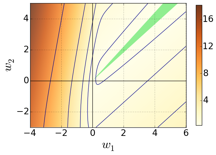
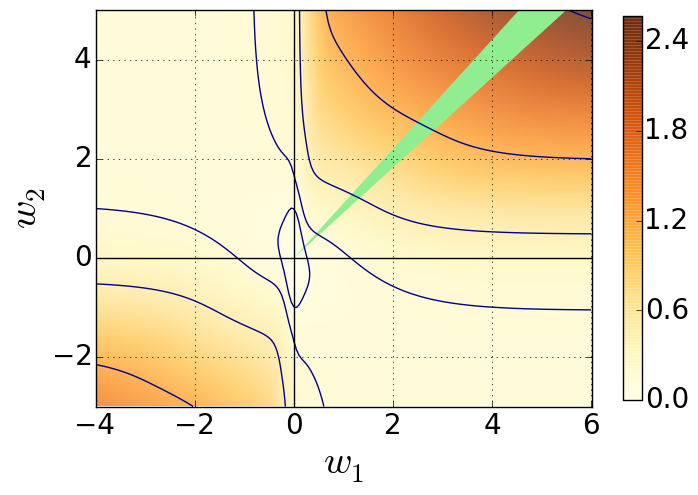
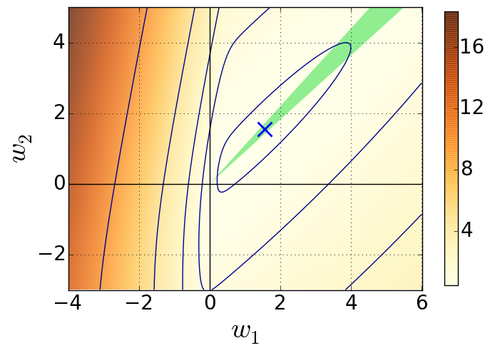
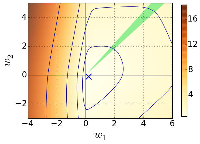
Figure 2: Using data favoring $L_{2}$ in (12). The expected loss is plotted in the upper-left, the dropout regularizer in the upper-right, the $L_{2}$ regularized criterion as in (5) in the lower-left and the dropout criterion as in (3) in the lower-right, all as functions of the weight vector. The Bayes-optimal weight vectors are in the green region, and “$\times$” marks show the optimizers of the criteria.

We first show that distribution $P_{\ref{s:2d.L2.wins}}$ of (12) is compatible with mild enough $L_{2}$ regularization. Recall that ${\bf v}(P_{\ref{s:2d.L2.wins}},\lambda)$ is weight vector found by minimizing the $L_{2}$ regularized criterion (5).

Theorem 16

If $0<\lambda\leq 1/50$, then $\mathrm{er}_{P_{\ref{s:2d.L2.wins}}}({\bf v}(P_{\ref{s:2d.L2.wins}},\lambda))=0$ for the distribution $P_{\ref{s:2d.L2.wins}}$ defined in (12).

In contrast, the ${\bf w}^{*}(P_{\ref{s:2d.L2.wins}},q)$ minimizing the dropout criterion (3) has error rate at least $1/3$.

Theorem 17

If $q\geq 1/3$ then $\mathrm{er}_{P_{\ref{s:2d.L2.wins}}}({\bf w}^{*}(P_{\ref{s:2d.L2.wins}},q))\geq 1/3$ for the distribution $P_{\ref{s:2d.L2.wins}}$ defined in (12).

The proofs of Theorem 16 and 17 are in Appendices D and E.

6 A source preferred by dropout

In this section, consider the joint distribution $P_{\ref{s:2d.drop.wins}}$ defined by

$$\begin{array}[]{cccc}x_{1}&x_{2}&y&{\bf Pr}({\bf x},y)\\ \hline\cr 1&0&1&3/7\\ -1/1000&1&1&3/7\\ 1/10&-1&1&1/7\end{array}$$ (13)

The intuition behind this distribution is that the $(1,0)$ data point encourages a large weight on the first feature. This means that the negative pressure on the second weight due to the $(1/10,-1)$ data point is much smaller (especially given its lower probability) than the positive pressure on the second weight due to the $(-1/1000,1)$ example. The $L_{2}$ regularized criterion emphasizes short vectors, and prevents the first weight from growing large enough (relative to the second weight) to correctly classify the $(1/10,-1)$ data point. On the other hand, the first feature is nearly perfect; it only has the wrong sign on the second example where it is $-\epsilon=-1/1000$. This means that, in light of Theorem 8 and Proposition 10, dropout will be much more willing to use a large weight for $x_{1}$, giving it an advantage for this source over $L_{2}$. The plots in Figure 3 illustrate this intuition.

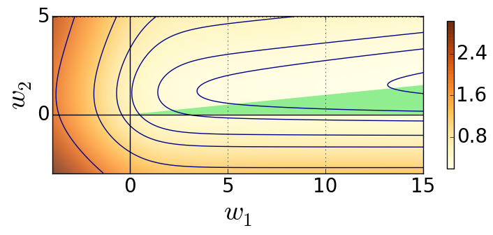
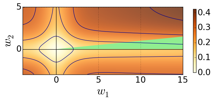
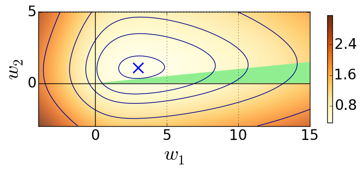
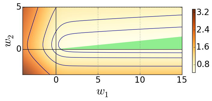
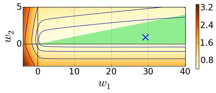
Figure 3: For the source from (13) favoring the dropout, the expected loss is plotted in the upper-left, the dropout regularizer in the upper-right, the expected loss plus $L_{2}$ regularization as in (5) in the lower-left and the dropout criterion as in (3) in the lower-right, all as functions of the weight vector. The Bayes-optimal weight vectors are in the green region, and “$\times$” marks show the optimizers of the criteria. Note that the minimizer of the dropout criterion lies outside the middle-right plot and is shown on the bottom plot (which has a different range and scale than the others.)

Theorem 18

If $1/100\leq\lambda\leq 1$, then $\mathrm{er}_{P_{\ref{s:2d.drop.wins}}}({\bf v}(P_{\ref{s:2d.drop.wins}},\lambda))\geq 1/7$ for the distribution $P_{\ref{s:2d.drop.wins}}$ defined in (13).

In contrast, the minimizer of the dropout criterion is able to generalize perfectly.

Theorem 19

If $q\leq 1/2$, then $\mathrm{er}_{P_{\ref{s:2d.drop.wins}}}({\bf w}^{*}(P_{\ref{s:2d.drop.wins}},q))=0.$ for the distribution $P_{\ref{s:2d.drop.wins}}$ defined in (13).

Theorems 18 and 19 are proved in Appendices F and G.

The results in this and the previous section show that the distributions defined in (12) and (13) strongly separate dropout and $L_{2}$ regularization. Theorem 19 shows that for distribution $P$ analyzed in this section $\mathrm{er}_{P}({\bf w}^{*}(P,q))=0$ for all $q\leq 1/2$ while Theorem 18 shows that for the same distribution $\mathrm{er}_{P}({\bf v}(P,\lambda)\geq 1/7$ whenever $\lambda\geq 1/100$. In contrast, when $Q$ is the distribution defined in the previous section, Theorem 16 shows $\mathrm{er}_{Q}({\bf v}(Q,\lambda))=0$ whenever $\lambda\leq 1/50$. For this same distribution $Q$, Theorem 17 shows that $\mathrm{er}_{Q}({\bf w}^{*}(Q,q))\geq 1/3$ whenever $q\geq 1/3$.

7 $L_{1}$ regularization

In this section, we show that the same $P_{\ref{s:2d.L2.wins}}$ and $P_{\ref{s:2d.drop.wins}}$ distributions that separate dropout from $L_{2}$ regularization also separate dropout from $L_{1}$ regularization: the algorithm the minimizes

$${\bf E}_{({\bf x},y)\sim P}(\ell(y{\bf w}\cdot{\bf x}))+\lambda||{\bf w}||_{1}.$$ (14)

  

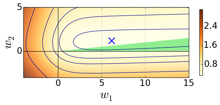
Figure 4: A plot of the $L_{1}$ criterion with $\lambda=0.01$ for distributions $P_{\ref{s:2d.L2.wins}}$ defined in Section 5 (left) and $P_{\ref{s:2d.drop.wins}}$ defined in Section 6 (right). As before, the Bayes optimal classifiers are denoted by the region shaded in green and the minimizer of the criterion is denoted with an x.

As in Sections 5 and 6, we set $\lambda=1/100$. Figure 4 plots the $L_{1}$ criterion (14) for the distributions $P_{\ref{s:2d.L2.wins}}$ defined in (12) and $P_{\ref{s:2d.drop.wins}}$ defined in (13). Like $L_{2}$ regularization, $L_{1}$ regularization produces a Bayes-opitmal classifier on $P_{\ref{s:2d.L2.wins}}$, but not on $P_{\ref{s:2d.drop.wins}}$. Therefore the same argument shows that these distributions also strongly separate dropout and $L_{1}$ regularization.

8 A high-dimensional source preferred by $L_{2}$

In this section we exhibit a source where $L_{2}$ regularization leads to a perfect predictor while dropout regularization creates a predictor with a constant error rate.

Consider the source $P_{\ref{s:L2.manyfeatures}}$ defined as follows. The number $n$ of features is even. All examples are labeled $1$. A random example is drawn as follows: the first feature takes the value $1$ with probability $9/10$ and $-1$ otherwise, and a subset of exactly $n/2$ of the remaining $n-1$ features (chosen uniformly at random) takes the value $1$, and the remaining $n/2-1$ of those first $n-1$ features take the value $-1$.

A majority vote over the last $n-1$ features achieves perfect prediction accuracy. This is despite the first feature (which does not participate in the vote) being more strongly correlated with the label than any of the voters in the optimal ensemble. Dropout, with its bias for single good features and discrimination against multiple disagreeing features, puts too much weight on this first feature. In contrast, $L_{2}$ regularization leads to the Bayes optimal classifier by placing less weight on the first feature than on any of the others.

Theorem 20

If $\lambda\leq\frac{1}{30n}$ then the weight vector $v(P_{\ref{s:L2.manyfeatures}},\lambda)$ optimizing the $L_{2}$ criterion has perfect prediction accuracy: $\mathrm{er}_{P_{\ref{s:L2.manyfeatures}}}(v(P_{\ref{s:L2.manyfeatures}},\lambda))=0$.

When $n>125$, dropout with $q=1/2$ fails to find the Bayes optimal hypothesis. In particular, we have the following theorem.

Theorem 21

If the dropout probability $q=1/2$ and the number of features is an even $n>125$ then the weight vector ${\bf w}^{*}(P_{\ref{s:L2.manyfeatures}},q)$ optimizing the dropout criterion has prediction error rate $\mathrm{er}_{P_{\ref{s:L2.manyfeatures}}}({\bf w}^{*}(P_{\ref{s:L2.manyfeatures}},q))\geq 1/10$.

We conjecture that dropout fails on $P_{\ref{s:L2.manyfeatures}}$ for all $n\geq 4$. As evidence, we analyze the $n=4$ case.

Theorem 22

If dropout probability $q=1/2$ and the number of features is $n=4$ then the minimizer of the dropout criteria ${\bf w}^{*}(P_{\ref{s:L2.manyfeatures}},q)$ has has prediction error rate $\mathrm{er}_{P_{\ref{s:L2.manyfeatures}}}({\bf w}^{*}(P_{\ref{s:L2.manyfeatures}},q))\geq 1/10$.

Theorems 20, 21 and 22 are proved in Appendices H, I and J.

9 A high-dimensional source preferred by dropout

Define the source $P_{\ref{s:dropout.wins.large.n}}$, which depends on (small) positive real parameters $\eta$, $\alpha$, and $\beta$, as follows. A random label $y$ is generated first, with both of $+1$ and $-1$ equally likely. The features $x_{1},...,x_{n}$ are conditionally independent given $y$. The first feature tends to be accurate but small: $x_{1}=\alpha y$ with probability $1-\eta$, and is $-\alpha y$ with probability $\eta$. The remaining features are larger but less accurate: for $2\leq i\leq n$, feature $x_{i}$ is $y$ with probability $1/2+\beta$, and $-y$ otherwise.

When $\eta$ is small enough relative to $\beta$, the Bayes’ optimal prediction is to predict with the first feature. When $\alpha$ is small, this requires concentrating the weight on $w_{1}$ to outvote the other features. Dropout is capable of making this one weight large while $L_{2}$ regularization is not.

Theorem 23

If $q=1/2$, $n\geq 100$, $\alpha>0$, $\beta=1/(10\sqrt{n-1})$, and $\eta\leq\frac{1}{2+\exp(54\sqrt{n})}$, then $\mathrm{er}_{P_{\ref{s:dropout.wins.large.n}}}({\bf w}^{*}(P_{\ref{s:dropout.wins.large.n}},q))=\eta.$

Theorem 24

If $\beta=1/(10\sqrt{n-1})$, $\lambda=\frac{1}{30n}$, $\alpha<\beta\lambda$, and $n$ is a large enough even number, then for any $\eta\in[0,1]$, $\mathrm{er}_{P_{\ref{s:dropout.wins.large.n}}}({\bf v}(P_{\ref{s:dropout.wins.large.n}},\lambda))\geq 3/10.$

Theorems 23 and 24 are proved in Appendices K and L.

Let $\tilde{n}$ be a large enough even number in the sense of Theorem 24. Let $P_{\eta}$ be the distribution defined at the start of Section 9 with number of features $n=\tilde{n}$, $\beta=1/(10\sqrt{n-1})$, $\alpha=1/(300n\sqrt{n})$, and $0<\eta<1/(2+\exp(54\sqrt{n}))$ is a free parameter. Theorem 23 shows that $\mathrm{er}_{P_{\eta}}({\bf w}^{*}(P_{\eta},q))=\eta$ when dropout probability $q=1/2$. For this same distribution, Theorem 24 shows $\mathrm{er}_{P_{\eta}}({\bf v}(P_{\eta},\lambda))\geq 3/10$ when $\lambda=1/30n$. Therefore

$$\frac{\mathrm{er}_{P_{\eta}}({\bf w}^{*}(P_{\eta},1/2))}{\mathrm{er}_{P_{\eta}}({\bf v}(P,1/30\tilde{n}))}$$

goes to 0 as $\eta\rightarrow 0$.

The distribution defined at the start of Section 8, which we call $Q$ here, provides contrasting behavior when $n=\tilde{n}$. Theorem 21 shows that the error $\mathrm{er}_{Q}({\bf w}^{*}(Q,1/2))\geq 1/10$ while Theorem 20 shows that $\mathrm{er}_{Q}(v(Q,1/30\tilde{n})=0$. Therefore the $P_{\eta}$ and $Q$ distributions strongly separate dropout and $L_{2}$ regularization for parameters $q=1/2$ and $\lambda=1/30n$.

10 Conclusions

We have built on the interpretation of dropout as a regularizer in Wager et al. (2013) to prove several interesting properties of the dropout regularizer. This interpretation decomposes the dropout criterion minimized by training into a loss term plus a regularization penalty that depends on the feature vectors in the training set (but not the labels). We started with a characterization of when the dropout criterion has a unique minimum, and then turn to properties of the dropout regularization penalty. We verified that the dropout regularization penalty has some desirable properties of a regularizer: it is 0 at the zero vector, and the contribution of each feature vector in the training set is non-negative.

On the other hand, the dropout regularization penalty does not behave like standard regularizers. In particular, we have shown:

1. Although the dropout “loss plus regularization penalty” criterion is convex in the weights ${\bf w}$, the regularization penalty imposed by dropout training is not convex.

2. Starting from an arbitrary weight vector, any single weight can go to infinity while the dropout regularization penalty remains bounded.

3. In some cases, multiple weights can simultaneously go to infinity while the regularization penalty remains bounded.

4. The regularization penalty can decrease as weights increase from 0 when the features are correlated.

These are in stark contrast to standard norm-based regularizers that always diverge as any weight goes to infinity, and are non-decreasing in each individual weight.

In most cases the dropout regularization penalty does diverge as multiple weights go to infinity. We characterize when sending two weights to infinity causes the dropout regularization penalty to diverge, and when it will remain finite. In particular, dropout is willing to put a large weights on multiple features if the $w_{i}x_{i}$ products tend to have the same sign.

The form of our analytical bounds suggest that the strength of the regularizer grows linearly with the dropout probability $q$, and provide additional support for the claim (Wager et al., 2013) that dropout favors rare features.

We found it important to check our intuition by working through small examples. To make this more rigorous we needed a definition of when a source favored dropout regularization over a more standard regularizer like $L_{2}$. Such a definition needs to deal with the strength of regularization, a difficulty complicated by the fact that dropout regularization is parameterized by the dropout probability $q\in[0,1]$ while $L_{2}$ regularization is parameterized by $\lambda\in[0,\infty]$. Our solution is to consider pairs of sources $P$ and $Q$. We then say the pair separates the dropout and $L_{2}$ if dropout with a particular parameter $q$ performs better then $L_{2}$ with a particular parameter $\lambda$ on source $P$, while $L_{2}$ (with the same $\lambda$) performs better than dropout (with the same $q$) on source $Q$. Our definition uses generalization error as the most natural interpretation of “performs better”.

Sections 5 through 9 are devoted to proving that dropout and $L_{2}$ are strongly separated by certain pairs of distributions. Section 7 shows that dropout and $L_{1}$ regularization are also strongly separated. Proving strong separation is non-trivial even after one finds the right distributions. This is due to several factors: the minimizers of the criteria do not have closed forms, we wish to prove separation for ranges of the regularization values, and the binomial distributions induced by dropout are not amenable to exact analysis. Despite these difficulties, the separation results reinforce the intuition that dropout is more willing to use a large weight in order to better fit the training data than $L_{2}$ regularization. However, if two features often have both the same and different signs (as in Theorem 13) then dropout is less willing to put even moderate weight on both features.

As a side benefit of these analyses, the plots in Figure 2 and Figure 3 provide a dramatic illustration of the dropout regularizer’s non-convexity and its preference for making only a single weight large. This is consistent with the insight provided by Theorems 13 and 15.

Our analysis is for the logistic regression case corresponding to a single output node. It would be very interesting to have similar analysis for multi-layer neural networks. However, dealing with non-convex loss of such networks will be a major challenge. Another open problem suggested by this work is how the definition of separation can be used to gain insight about other regularizers and settings.

Appendix A Proof of Proposition 12

Proposition 12. Fix $p=1/2$, $w_{2}>0$, and an arbitrary ${\bf x}\in(0,\infty)^{2}$. Let $D$ be the distribution concentrated on ${\bf x}$. Then $\mathrm{reg}_{D,q}(w_{1},w_{2})$ locally decreases as $w_{1}$ increases from $0$.

First, we show that assuming ${\bf x}=(2,2)$ is without loss of generality. When $D$ concentrates all of its probability on a single ${\bf x}$, let us denote $\mathrm{reg}_{D,1/2}$ by $\mathrm{reg}_{{\bf x},1/2}$. Since anyplace $w_{1}$ appears in the expression for $\mathrm{reg}_{{\bf x},1/2}$, it is multiplied by $x_{1}$, if we multiply $w_{1}$ by some constant $c$ and divide $x_{1}$ by $c$, we do not change $w_{1}x_{1}$, and therefore do not change $\mathrm{reg}_{{\bf x},1/2}$. The same holds for $w_{2}$. Thus

$$\mathrm{reg}_{{\bf x},1/2}({\bf w})=\mathrm{reg}_{(2,2),1/2}(w_{1}x_{1}/2,w_{2}x_{2}/2).$$

If we change variables and let $\tilde{w}_{1}=w_{1}x_{1}/2$ and $\tilde{w}_{2}=w_{2}x_{2}/2$, then since $x_{1}$ and $x_{2}$ are both positive, $\tilde{w}_{2}$ is positive iff $w_{2}$ is, and $\mathrm{reg}_{{\bf x},1/2}({\bf w})$ is increasing with $w_{1}$ iff $\mathrm{reg}_{(2,2),1/2}(\tilde{{\bf w}})$ is increasing with $\tilde{w}_{1}$.

We continue assuming ${\bf x}=(2,2)$. It suffices to show $\partial\mathrm{reg}_{D,q}(w_{1},w_{2})/\partial w_{1}|_{w_{1}=0}<0$. This derivative is

$$\frac{3e^{w_{2}}+e^{-3w_{2}}-3e^{-w_{2}}-e^{3w_{2}}}{2(e^{w_{2}}+e^{-w_{2}})(e^{2w_{2}}+e^{-2w_{2}})}.$$ (15)

The sign depends only on the numerator, which is $0$ when $w_{2}=0$. The derivative of the numerator with respect to $w_{2}$ is $3e^{w_{2}}-3e^{-3w_{2}}+3e^{-w_{2}}-3e^{3w_{2}}$, which is negative for $w_{2}>0$, since $e^{z}+e^{-z}$ is an increasing function in $z$. Thus the numerator in (15) is decreasing in $w_{2}$. Therefore (15) is negative when $w_{2}>0$, and the regularization penalty is (locally) decreasing as $w_{1}$ increases from 0.

(Note: Proposition 12 may be generalized with slight modifications to apply whenever ${\bf x}$ has two nonzero components. What is needed is that $x_{1}w_{1}$ and $x_{2}w_{2}$ have the same sign. For example, if $x_{1}$ is negative but $x_{2}w_{2}$ is positive, then moving $w_{1}$ from $0$ in the negative direction decreases $\mathrm{reg}_{D,q}({\bf w})$.)

Appendix B Proof of Theorem 13

Theorem 13. Fix an arbitrary distribution $D$ with support in ${\bf R}^{2}$, weight vector ${\bf w}\in{\bf R}^{2}$, and non-dropout probability $p$. If there is an ${\bf x}$ with positive probability under $D$ such that $w_{1}x_{1}$ and $w_{2}x_{2}$ are both non-zero and have different signs, then the regularization penalty $\mathrm{reg}_{D,q}(\omega{\bf w})$ goes to infinity as $\omega$ goes to $\pm\infty$.

Fix an ${\bf x}$ satisfying the conditions of the theorem.

$$\mathrm{reg}_{D,q}(\omega{\bf w}) \geq D({\bf x}){\bf E}_{{\boldsymbol{\nu}}}\left(\ln\left(\frac{\exp(-\frac{\omega{\bf w}\cdot({\bf x}+{\boldsymbol{\nu}})}{2})+\exp(\frac{\omega{\bf w}\cdot({\bf x}+{\boldsymbol{\nu}})}{2})}{\exp(\frac{-\omega{\bf w}\cdot{\bf x}}{2})+\exp(\frac{\omega{\bf w}\cdot{\bf x}}{2})}\right)\right)$$

$$>D({\bf x}){\bf E}_{{\boldsymbol{\nu}}}\left(\ln\left(\frac{\exp(\frac{|\omega{\bf w}\cdot({\bf x}+{\boldsymbol{\nu}})|}{2})}{2\exp(\frac{|\omega{\bf w}\cdot{\bf x}|}{2})}\right)\right)$$

$$=D({\bf x}){\bf E}_{{\boldsymbol{\nu}}}\left(-\ln(2)+\frac{|\omega{\bf w}\cdot({\bf x}+{\boldsymbol{\nu}})|}{2}-\frac{|\omega{\bf w}\cdot{\bf x}|}{2}\right).$$ (16)

We now examine the expectation over ${\boldsymbol{\nu}}$ of the term that depends on ${\boldsymbol{\nu}}$. We assume that $|w_{1}x_{1}|\geq|w_{2}x_{2}|$ so $|{\bf w}\cdot{\bf x}|=|w_{1}x_{1}|-|w_{2}x_{2}|$; the other case is symmetrical.

$${\bf E}_{{\boldsymbol{\nu}}}(|\omega{\bf w}\cdot({\bf x}+{\boldsymbol{\nu}})|) =|\omega|\big{(}p^{2}|{\bf w}\cdot{\bf x}/p|+p(1-p)|w_{1}x_{1}/p|+p(1-p)|w_{2}x_{2}/p|\big{)}$$

$$=|\omega|\big{(}p|{\bf w}\cdot{\bf x}|+(1-p)(|w_{1}x_{1}|-|w_{2}x_{2}|+|w_{2}x_{2}|)+(1-p)|w_{2}x_{2}|\big{)}$$

$$=|\omega|(|{\bf w}\cdot{\bf x}|+2(1-p)|w_{2}x_{2}|).$$

Plugging this into (16) gives:

$$\mathrm{reg}_{D,q}(\omega{\bf w})>D({\bf x})\left(-\ln 2+(1-p)|\omega||w_{2}x_{2}|\right)$$

which goes to infinity as $\omega$ goes to $\pm\infty$.

Appendix C Proof of Theorem 15

Theorem 15. Let ${\bf w}$ be a weight vector and $D$ be a discrete distribution such that $w_{i}x_{i}\geq 0$ for each index $i$ and all ${\bf x}$ in the support of $D$. The limit of $\mathrm{reg}_{D,q}(\omega{\bf w})$ as $\omega$ goes to infinity is bounded by $\ln(2)(1-p){\bf P}_{{\bf x}\sim D}({\bf w}\cdot{\bf x}\neq 0)$.

First note that If ${\bf w}$ and $D$ are such that ${\bf w}\cdot{\bf x}=0$ for all ${\bf x}$ in the support of $D$, then $\mathrm{reg}_{D,q}({\bf w})=\mathrm{reg}_{D,q}(\omega{\bf w})=0$. We now analyze the general case.

$$\mathrm{reg}_{D,q}(\omega{\bf w})\ ={\bf E}_{{\bf x},{\boldsymbol{\nu}}}\left(\ln\left(\frac{\exp(\frac{\omega{\bf w}\cdot({\bf x}+{\boldsymbol{\nu}})}{2})+\exp(\frac{-\omega{\bf w}\cdot({\bf x}+{\boldsymbol{\nu}})}{2})}{\exp(\frac{\omega{\bf w}\cdot{\bf x}}{2})+\exp(\frac{-\omega{\bf w}\cdot{\bf x}}{2})}\right)\right)$$

$$={\bf E}_{{\bf x},{\boldsymbol{\nu}}}\left(\ln\left(\frac{\exp(\frac{\omega{\bf w}\cdot({\bf x}+\nu)}{2})(1+\exp(-\omega{\bf w}\cdot({\bf x}+{\boldsymbol{\nu}})))}{\exp(\frac{\omega{\bf w}\cdot{\bf x}}{2})(1+\exp(-\omega{\bf w}\cdot{\bf x}))}\right)\right)$$

$$={\bf E}_{{\bf x},{\boldsymbol{\nu}}}\Big{(}\left(\omega{\bf w}\cdot({\bf x}+{\boldsymbol{\nu}})/2\right)+\ln\left(1+\exp\left(-\omega{\bf w}\cdot({\bf x}+{\boldsymbol{\nu}})\right)\right)$$

$$\qquad-\left(\omega{\bf w}\cdot{\bf x}/2\right)-\ln\left(1+\exp\left(-\omega{\bf w}{\bf x}\right)\right)\Big{)}.$$ (17)

Of the four terms inside the expectation in Equation (17), the first and third cancel since the expectation of ${\boldsymbol{\nu}}$ is ${\boldsymbol{0}}$. Therefore:

$$\mathrm{reg}_{D,q}(\omega{\bf w})={\bf E}_{{\bf x}}\big{(}{\bf E}_{\boldsymbol{\nu}}\big{(}\ln(1+\exp(-\omega{\bf w}\cdot({\bf x}+{\boldsymbol{\nu}})))-\ln(1+\exp(-\omega{\bf w}{\bf x}))\big{)}\big{)}.$$ (18)

Define $\text{nez}({\bf w},{\bf x})$ to be the number of indices $i$ where $w_{i}x_{i}\neq 0$. We now consider cases based on $\text{nez}({\bf w},{\bf x})$.

Whenever $\text{nez}({\bf w},{\bf x})=0$ then both ${\bf w}\cdot{\bf x}=0$ and ${\bf w}\cdot({\bf x}+{\boldsymbol{\nu}})=0$. Therefore the contribution of these ${\bf x}$ to the expectation in (18) is $\ln(2)-\ln(2)=0$.

If $\text{nez}({\bf w},{\bf x})>0$ then ${\bf w}\cdot{\bf x}>0$ (since each $w_{i}x_{i}\geq 0$), and the second term of (18) goes to zero as $\omega$ goes to infinity. The first term of (18) also goes to zero, unless all of the $\text{nez}({\bf w},{\bf x})$ components where $w_{i}x_{i}>0$ are dropped out. If they are all dropped out, then the first term becomes $\ln(2)$. The probability that all $\text{nez}({\bf w},{\bf x})$ non-zero components are simultaneously dropped out is $(1-p)^{\text{nez}({\bf w},{\bf x})}$. With this reasoning we get from (18) that:

$$\lim_{\omega\rightarrow\infty}\mathrm{reg}_{D,q}(\omega{\bf w})$$

$$=\sum_{k=1}^{n}{\bf P}_{{\bf x}\sim D}(\text{nez}({\bf w},{\bf x})=k)\left(\ln(2)(1-p)^{k}\right)$$ (19)

$$\leq\sum_{k=1}^{n}{\bf P}_{{\bf x}\sim D}(\text{nez}({\bf w},{\bf x})=k)\left(\ln(2)(1-p)\right)$$

$$=\ln(2)(1-p){\bf P}({\bf w}\cdot{\bf x}\neq 0)$$

as desired.

(Note that Equation 19 gives a precise, but more complex expression for the limit.)

Appendix D Proof of Theorem 16

Theorem 16. If $0<\lambda\leq 1/50$, then $\mathrm{er}_{P_{\ref{s:2d.L2.wins}}}({\bf v}(P_{\ref{s:2d.L2.wins}},\lambda))=0$ for the distribution $P_{\ref{s:2d.L2.wins}}$ defined in (12).

To keep the notation clean let us abbreviate $P_{\ref{s:2d.L2.wins}}$ as just $P$ throughout this proof.

By scaling the $L_{2}$ criterion we can obtain cancellation in the expectation. Let ${\bf v}$ be weight vector found by minimizing the following $L_{2}$ regularized criterion $J$:

$$J({\bf w})=3\left({\bf E}_{({\bf x},y)\sim P}(\ell(y({\bf w}\cdot{\bf x})))+(\lambda/2)||{\bf w}||^{2}\right).$$ (20)

Note the factor of 3 is to simplify the expressions and doesn’t affect the minimizing ${\bf v}$.

We will prove Theorem 16 with a series of lemmas.

But first, let’s take some partial derivatives:

$$\frac{\partial J}{\partial w_{1}} =\frac{-10}{1+\exp(10w_{1}-w_{2})}+\frac{-1.1}{1+\exp(1.1w_{1}-w_{2})}+\frac{1}{1+\exp(-w_{1}+1.1w_{2})}+3\lambda w_{1}$$ (21)

$$\frac{\partial J}{\partial w_{2}} =\frac{1}{1+\exp(10w_{1}-w_{2})}+\frac{1}{1+\exp(1.1w_{1}-w_{2})}+\frac{-1.1}{1+\exp(-w_{1}+1.1w_{2})}+3\lambda w_{2}.$$ (22)

We will repeatedly use the following basic, well-known, lemma.

Lemma 25

For any convex, differentiable function $\psi$ defined on ${\bf R}^{n}$ with a unique minimum ${\bf w}^{*}$, for any ${\bf w}\in{\bf R}^{n}$, if $g({\bf w})$ is the gradient of $\psi$ at ${\bf w}$ then ${\bf w}^{*}$ is contained in the closed halfspace whose separating hyperplane goes through ${\bf w}$, and whose normal vector is $-g({\bf w})$; i.e., ${\bf w}^{*}\cdot g({\bf w})\leq{\bf w}\cdot g({\bf w})$. Furthermore, if $g({\bf w})\neq{\boldsymbol{0}}$ then ${\bf w}^{*}\cdot g({\bf w})<{\bf w}\cdot g({\bf w})$.

Now we’re ready to start our analysis of $P$.

Lemma 26

If $0\leq\lambda$, the optimizing $v_{1}$ is positive.

Proof: By Lemma 25, it suffices to show that there is a point $(0,a_{2})$ where both $\frac{\partial J}{\partial w_{1}}\big{|}_{(0,a_{2})}<0$ and $\frac{\partial J}{\partial w_{2}}\big{|}_{(0,a_{2})}=0$.

From Equation (21):

$$\frac{\partial J}{\partial w_{1}}\Bigg{|}_{(0,a_{2})}=\frac{-11.1}{1+\exp(-a_{2})}+\frac{1}{1+\exp(1.1a_{2})}$$

and each term is decreasing as $a_{2}$ increases. Since it is negative when $a_{2}=-2$, we have $\frac{\partial J}{\partial w_{1}}\Big{|}_{(0,a_{2})}<0$ for all $a_{2}>-2$. So, to prove the lemma, if suffices to show that there is a $a_{2}\in(-2,\infty)$ such that the other derivative $\frac{\partial J}{\partial w_{2}}\Big{|}_{(0,a_{2})}=0$.

From equation (22):

$$\frac{\partial J}{\partial w_{2}}\Big{|}_{(0,a_{2})}=\frac{2}{1+\exp(-a_{2})}+\frac{-1.1}{1+\exp(1.1a_{2})}+3\lambda a_{2}$$

and each term is continuously increasing in $a_{2}$. When $a_{2}=-2$, $\frac{\partial J}{\partial w_{2}}\Big{|}_{(0,a_{2})}$ is negative. On the other hand, $\frac{\partial J}{\partial w_{2}}\big{|}_{(0,0)}$ is positive. Therefore for some $a_{2}\in(-2,0)$ we have $\frac{\partial J}{\partial w_{2}}\big{|}_{(0,a_{2})}=0$ as desired.  

Lemma 27

There is a real $a>0$ such that

$$\frac{\partial J({\bf w})}{\partial w_{1}}\Bigg{|}_{(a,a)}+\frac{\partial J({\bf w})}{\partial w_{2}}\Bigg{|}_{(a,a)}=0.$$

Proof: Applying (21) and (22), we get

$$b\stackrel{{\scriptstyle\textup{def}}}{{=}}\frac{\partial J({\bf w})}{\partial w_{1}}\Bigg{|}_{(a,a)}+\frac{\partial J({\bf w})}{\partial w_{2}}\Bigg{|}_{(a,a)}=\displaystyle{\frac{-9}{1+\exp(9a)}+\frac{-0.2}{1+\exp(a/10)}+6\lambda a}.$$

Since $b$ is negative when $a=0$ and is a continuous function of $a$, and $\lim_{a\rightarrow\infty}b>\infty$, the lemma holds.  

Lemma 28

$v_{1}\geq v_{2}$.

Proof: Let $a$ be the value from Lemma 27, and let ${\bf g}=(g_{1},g_{2})$ be the gradient of $J$ at $(a,a)$. Lemma 25 implies that ${\bf v}$ lies in the halfspace through $(a,a)$ in the direction of $-{\bf g}$. Lemma 27 implies that

$$g_{1}=\frac{\partial J({\bf w})}{\partial w_{1}}\Bigg{|}_{(a,a)}=-\frac{\partial J({\bf w})}{\partial w_{2}}\Bigg{|}_{(a,a)}=-g_{2}.$$

Examination of the derivatives (21) and (22) at $(a,a)$ shows that the first term of (21) is negative and the first term of (22) is positive while the last three terms match (although in a different order). Therefore $g_{1}<0$ and $g_{2}=-g_{1}$ is positive. Applying Lemma 25 completes the proof.  

Lemma 28 implies that ${\bf v}$ correctly classifies $(10,-1)$ and $(11/10,-1)$. It remains to show that ${\bf v}$ correctly classifies $(-1,11/10)$, that is, that $v_{1}$ is not too much bigger than $v_{2}$.

Lemma 29

If $v_{2}\geq 0.6$ and $\lambda>0$ then $v_{1}<11v_{2}/10$.

Proof: Combining $\frac{\partial J}{\partial w_{1}}\Big{|}_{{\bf v}}=0$ with (21), we get

$$3\lambda v_{1}=\frac{10}{1+\exp(10v_{1}-v_{2})}+\frac{1.1}{1+\exp(1.1v_{1}-v_{2})}+\frac{-1}{1+\exp(-v_{1}+1.1v_{2})}$$

and, similarly,

$$3\lambda v_{2}=\frac{-1}{1+\exp(10v_{1}-v_{2})}+\frac{-1}{1+\exp(1.1v_{1}-v_{2})}+\frac{1.1}{1+\exp(-v_{1}+1.1v_{2})}.$$

Thus

$$3\lambda(10v_{1}-11v_{2})=\frac{111}{1+\exp(10v_{1}-v_{2})}+\frac{22}{1+\exp(1.1v_{1}-v_{2})}-\frac{22.1}{1+\exp(-v_{1}+1.1v_{2})}.$$ (23)

Assume for contraction that $v_{1}\geq 11v_{2}/10$. Then $10v_{1}-v_{2}\geq 10v_{2}$, $1.1v_{1}-v_{2}\geq 0.21v_{2}$, and $-v_{1}+1.1v_{2}\leq 0$, so

$$3\lambda(10v_{1}-11v_{2})\leq\frac{111}{1+\exp(10v_{2})}+\frac{22}{1+\exp(0.21v_{2})}-11.05.$$

However, $10v_{1}-11v_{2}\geq 0$ and (since $v_{2}\geq 0.6$) the RHS is negative, giving the desired contradiction.  

Lemma 30

If $0<\lambda\leq 1/50$ then $v_{2}\geq 0.6$.

Proof: It suffices to show that there is a point $(x,0.6)$ where the partial w.r.t. $w_{1}$ is 0 and the partial w.r.t $w_{2}$ is negative.

$$\frac{\partial J}{\partial w_{1}}\Big{|}_{(x,0.6)}=\frac{-10}{1+\exp(10x-0.6)}+\frac{-1.1}{1+\exp(1.1x-0.6)}+\frac{1}{1+\exp(-x+0.66)}+3\lambda x$$

and is increasing in $x$ and $\lambda$ (assuming $x>0$) and becomes positive as $x$ goes to infinity. It is negative when evaluated at $x=0.6$ and $\lambda=1/50$, so for all $\lambda\leq 1/50$ there is an $x>1$ such that $\partial J/\partial w_{+}\big{|}_{(x,1)}=0$.

$$\frac{\partial J}{\partial w_{2}}\Big{|}_{(x,0.6)}=\frac{1}{1+\exp(10x-0.6)}+\frac{1}{1+\exp(1.1x-0.6)}+\frac{-1.1}{1+\exp(-x+0.66)}+1.8\lambda\\$$

and is decreasing in $x$ and increasing in $\lambda$. It is negative when $x=1$ and $\lambda=1/50$, so it will remain negative for all $x>1$ and $0\leq\lambda\leq 1/50$, as desired.  

So, we have shown that, if $\lambda\leq 1/50$, then all examples are classified correctly by ${\bf v}$, which proves Theorem 16.

Appendix E Proof of Theorem 17

Theorem 17. If $q\geq 1/3$ then $\mathrm{er}_{P_{\ref{s:2d.L2.wins}}}({\bf w}^{*}(P_{\ref{s:2d.L2.wins}},q))\geq 1/3$ for the distribution $P_{\ref{s:2d.L2.wins}}$ defined in (12).

Throughout this proof we also abbreviate $P_{\ref{s:2d.L2.wins}}$ as just $P$.

For this subsection, let us define the scaled dropout criterion

$$J({\bf w})=3\;{\bf E}_{({\bf x},y)\sim P,{\bf r}}(\ell(y({\bf w}\cdot({\bf r}\odot{\bf x}))))$$ (24)

where the components of ${\bf r}$ are independent samples from a Bernoulli distribution with parameter $p=1-q>0$. Again, the factor of 3 is to simplify the expectation and doesn’t change the minimizing ${\bf w}$. Let ${\bf w}^{\circledast}$ be the minimizer of this $J({\bf w})$, so that Equation (4) implies that the optimizer ${\bf w}^{*}$ of the dropout criterion is $p{\bf w}^{\circledast}$. Note that ${\bf w}^{*}$ classifies an example correctly if and only if ${\bf w}^{\circledast}$ does.

Next, note that we may assume without loss of generality that both components of ${\bf w}^{\circledast}$ are positive, since, if either is negative, one of $(-1,1.1)$ or $(1.1,-1)$ is misclassified and we are done.

We will prove Theorem 17 by proving that, when $q\geq 1/3$, ${\bf w}^{\circledast}$ misclassifies $(-1,1.1)$, or, equivalently, that $w^{\circledast}_{1}>(11/10)w^{\circledast}_{2}$.

First, let us evaluate some partial derivatives. (Note that, if $x_{i}$ is dropped out, the value of $w_{i}$ does not matter.)

$$\frac{\partial J}{\partial w_{1}} =(1-q)^{2}\left(\frac{-10}{1+\exp(10w_{1}-w_{2})}+\frac{-1.1}{1+\exp(1.1w_{1}-w_{2})}+\frac{1}{1+\exp(-w_{1}+1.1w_{2})}\right)$$ (25)

$$\hskip 14.45377pt+(1-q)q\left(\frac{-10}{1+\exp(10w_{1})}+\frac{-1.1}{1+\exp(1.1w_{1})}+\frac{1}{1+\exp(-w_{1})}\right)$$

$$\frac{\partial J}{\partial w_{2}} =(1-q)^{2}\left(\frac{1}{1+\exp(10w_{1}-w_{2})}+\frac{1}{1+\exp(1.1w_{1}-w_{2})}+\frac{-1.1}{1+\exp(-w_{1}+1.1w_{2})}\right)$$ (26)

$$\hskip 14.45377pt+q(1-q)\left(\frac{1}{1+\exp(-w_{2})}+\frac{1}{1+\exp(-w_{2})}+\frac{-1.1}{1+\exp(1.1w_{2})}\right).$$

The following is the key lemma. As before, it is useful since, for any ${\bf w}$, if $g({\bf w})$ is nonzero, then ${\bf w}^{\circledast}$ lies in the open halfspace through ${\bf w}$ whose normal vector is the negative gradient.

Lemma 31

For all $a>0$ and $q\geq 1/3$,

$$\frac{\partial J}{\partial w_{2}}\Bigg{|}_{(a,10a/11)}>0.$$ (27)

Proof: We have

$$\frac{\partial J}{\partial w_{2}}\Bigg{|}_{(a,10a/11)}= (1-q)^{2}\left(\frac{1}{1+\exp(100a/11)}+\frac{1}{1+\exp(21a/110)}+\frac{-1.1}{2}\right)$$

$$+q(1-q)\left(\frac{2}{1+\exp(-10a/11)}+\frac{-1.1}{1+\exp(a)}\right).$$

Note that this derivative is positive if and only if

$$f(q,a)= \left(\frac{1}{1-q}\right)\;\frac{\partial J}{\partial w_{2}}\Bigg{|}_{(a,10a/11)}$$

$$= q\left(\frac{11}{20}+\frac{2}{1+\exp(-10a/11)}+\frac{-1}{1+\exp(21a/110)}+\frac{-1}{1+\exp(100a/11)}+\frac{-11/10}{1+\exp(a)}\right)$$

$$\hskip 14.45377pt+\frac{1}{1+\exp(21a/110)}+\frac{1}{1+\exp(100a/11)}+\frac{-11}{20}$$

is positive, as $0<q<1$. Note that the terms multiplying $q$ are increasing in $a$ and sum to 0 when $a=0$. On the other hand, the terms not multiplied by $q$ are decreasing in $a$ and turn negative when $a$ is just over $1/4$. Thus both parts are positive when $a\leq 1/4$. Note that $f(q,a)$ can be underestimated by underestimating $a$ on the $q$-terms and overestimating $a$ on the other terms.

For $1/4\leq a\leq 2$,

$$f(q,a)\geq q\left(\frac{11}{20}+\frac{2}{1+\exp(-10/44)}+\frac{-1}{1+\exp(21/440)}+\frac{-1}{1+\exp(100/44)}+\frac{-11/10}{1+\exp(1/4)}\right)$$

$$+\frac{1}{1+\exp(42/110)}+\frac{1}{1+\exp(200/11)}+\frac{-11}{20}$$

$$\geq 0.5q-0.15$$

and is positive whenever $q\geq 1/3$.

For $a\geq 2$,

$$f(q,a) \geq q\left(\frac{11}{20}+\frac{2}{1+\exp(-20/11)}+\frac{-1}{1+\exp(42/110)}+\frac{-1}{1+\exp(200/11)}+\frac{-11/10}{1+\exp(2)}\right)+\frac{-11}{20}$$

$$\geq 1.7q-11/20$$

and is also positive whenever $q\geq 1/3$.  

Proof of Theorem 17: Let ${\bf g}=(g_{1},g_{2})$ be the gradient of $J$ at $(w_{1}^{\circledast},10w_{1}^{\circledast}/11)$. Lemma 31 shows ${\bf g}$ is not ${\bf 0}$, so by convexity

$${\bf w}^{\circledast}\cdot{\bf g}<(w_{1}^{\circledast},10w_{1}^{\circledast}/11)\cdot{\bf g}$$

which implies

$$w_{2}^{\circledast}\;g_{2}<(10w_{1}^{\circledast}/11)\;g_{2}.$$

Since $g_{2}>0$ (Lemma 31), this implies

$$w_{2}^{\circledast}<(10w_{1}^{\circledast}/11)$$

and the $(-1,11/10)$ example is misclassified by ${\bf w}^{\circledast}$, and therefore by ${\bf w}^{*}$, completing the proof.  

Appendix F Proof of Theorem 18

Theorem 18. If $1/100\leq\lambda\leq 1$, then $\mathrm{er}_{P_{\ref{s:2d.drop.wins}}}({\bf v}(P_{\ref{s:2d.drop.wins}},\lambda))\geq 1/7$ for the distribution $P_{\ref{s:2d.drop.wins}}$ defined in (13).

To keep the notation clean, in this section let us abbreviate $P_{\ref{s:2d.drop.wins}}$ simply as $P$.

As the reader might expect, we will prove Theorem 18 by proving that ${\bf v}$ fails to correctly classify $(1/10,-1)$, that is, by proving that $v_{1}<10v_{2}$.

We may assume that $v_{1}>0$, since, otherwise, $(1,0)$ is misclassified.

To obtain cancellation in the expectation, we work with the scaled $L_{2}$ criterion

$$J({\bf w})=7{\bf E}_{({\bf x},y)\sim P}(\ell(y({\bf w}\cdot{\bf x})))+(7\lambda/2)||{\bf w}||^{2}.$$ (28)

and let ${\bf v}(P,\lambda)$ be the vector minimizing this $J$, which we often abbreviate as simply ${\bf v}$, leaving it implicitly a function of $\lambda$. Note that this scaling of the criteria does not change the minimizing ${\bf v}$.

Taking derivatives,

$$\frac{\partial J}{\partial w_{1}} =\frac{-3}{1+\exp(w_{1})}+\frac{3\epsilon}{1+\exp(-\epsilon w_{1}+w_{2})}+\frac{-0.1}{1+\exp(w_{1}/10-w_{2})}+7\lambda w_{1}$$ (29)

$$\frac{\partial J}{\partial w_{2}} =\frac{-3}{1+\exp(-\epsilon w_{1}+w_{2})}+\frac{1}{1+\exp(w_{1}/10-w_{2})}+{7\lambda w_{2}}.$$ (30)

Lemma 32

If either: $\lambda\geq 1/100$ and $a\geq 1/3$, or $\lambda\geq 1/4$ and $a\geq 1/15$ then

$$\frac{\partial J({\bf w})}{\partial w_{1}}\Big{|}_{(10a,a)}>0.$$

Proof: We have

$$\frac{\partial J({\bf w})}{\partial w_{1}}\Bigg{|}_{(10a,a)}=\frac{-3}{(1+\exp(10a))}+\frac{3\epsilon}{1+\exp((1-10\epsilon)a)}+\frac{-1}{20}+70\lambda a>\frac{-3}{(1+\exp(10a))}+\frac{-1}{20}+70\lambda a.$$

Each term of the RHS is non-decreasing in $a$ and $\lambda$, and the RHS is positive when either $\lambda=1/100$ and $a=1/3$ or $\lambda=1/4$ and $a=1/15$.  

To apply this, we want to show that $v_{2}$ is large enough, which we do next.

Lemma 33

If $\lambda\leq 1/4$ then $v_{2}\geq 1/3$ and if $\lambda\leq 1$ then $v_{2}\geq 1/15$.

Proof: Assume to the contrary that $\lambda\leq 1/4$ but $v_{2}<1/3$. From (30), and using that $v_{1}>0$, we have

$$\frac{\partial J}{\partial w_{2}}\Bigg{|}_{{\bf v}}<\frac{-3}{1+\exp(v_{2})}+\frac{1}{1+\exp(-v_{2})}+{7\lambda v_{2}},$$ (31)

a bound that is increasing in $v_{2}$ and $\lambda$. Since $\frac{\partial J}{\partial w_{2}}\Big{|}_{{\bf v}}=0$, the bound must be positive. However, when $v_{2}\leq 1/3$ and $\lambda\leq 1/4$, it is negative, giving the desired contradiction.

Since the bound (31) is also negative at $v_{2}=1/15$ and $\lambda=1$, a similar contradiction proves the other half of the lemma.  

Proof: (of Theorem 18): Lemmas 32 and 33 imply that $(10v_{2},v_{2})$ is not the minimizing ${\bf v}$ (when $\lambda\geq 1/100$), so by convexity,

$$J(10v_{2},v_{1})+\bigl{(}(v_{1},v_{2})-(10v_{2},v_{2})\bigr{)}\cdot\nabla J(10v_{2},v_{2}) <J(v_{1},v_{2})$$ (32)

$$(v1-10v_{2})\ \frac{\partial J}{\partial w_{2}}\Bigg{|}_{(10v_{2},v_{2})} <0.$$ (33)

If $1/100\leq\lambda\leq 1/4$ then Lemma 33 shows that $v_{2}\geq 1/3$ and if $1/4\leq\lambda\leq 1$ then it shows that $v_{2}\geq 1/15$. In either case, Lemma 32 shows that that $\frac{\partial J}{\partial w_{2}}\Big{|}_{(10v_{2},v_{2})}>0$. Therefore,

$$v_{1}<10v_{2}$$

and $(0.1,-1)$ is misclassified by ${\bf v}$, completing the proof.  

Appendix G Proof of Theorem 19

Theorem 19. If $q\leq 1/2$, then $\mathrm{er}_{P_{\ref{s:2d.drop.wins}}}({\bf w}^{*}(P_{\ref{s:2d.drop.wins}},q))=0.$ for the distribution $P_{\ref{s:2d.drop.wins}}$ defined in (13).

In this proof, let us abbreviate $P_{\ref{s:2d.drop.wins}}$ with just $P$, and use $\epsilon$ to denote $1/1000$.

Table 2: Seven times the dropout distribution. The three probability sub-columns correspond to the original examples (1,0), (-1/1000, 1), (1/10, -1), and the final column is the over-estimate used in Lemma 36.

$$\begin{array}[]{ | c c | c | c c c | c |}\hline\cr{x_{1}r_{1}}&{x_{2}r_{2}}&{y}&\lx@intercol\hfil\mbox{seven times probability}\hfil\lx@intercol\vrule\lx@intercol&\mbox{${\bf w}^{\circledast}\cdot({\bf r}\odot{\bf x})$ over-estimate}\\ \hline\cr 0&0&1&3q&+3q^{2}&+q^{2}&0\\ 1&0&1&3(1-q)&&&\infty\\ 0&1&1&&3q(1-q)&&w_{2}\\ -1/1000&0&1&&3q(1-q)&&0\\ -1/1000&1&1&&3(1-q)^{2}&&w_{2}\\ 0&-1&1&&&q(1-q)&\infty\\ 1/10&0&1&&&q(1-q)&\infty\\ 1/10&-1&1&&&(1-q)^{2}&\infty\\ \hline\cr\end{array}$$

For this section, let us define the scaled dropout criterion

$$J({\bf w})=7{\bf E}_{({\bf x},y)\sim P,{\bf r}}(\ell(y({\bf w}\cdot({\bf r}\odot{\bf x})))),$$ (34)

where, as earlier, the components of ${\bf r}$ are independent samples from a Bernoulli distribution with parameter $p=1-q=1/2>0$. (Note that, similarly to before, scaling up the objective function by 7 does not change the minimizer of $J$.) See Table 2 for a tabular representation of the distribution after dropout. Let ${\bf w}^{\circledast}$ be the minimizer of $J$, so that ${\bf w}^{*}=p{\bf w}^{\circledast}$ (see Equation (4)).

First, let us evaluate some partial derivatives (note that $1-q=(1-q)^{2}+q(1-q)$).

$$\frac{\partial J}{\partial w_{1}} =(1-q)^{2}\left(\frac{-3}{1+\exp(w_{1})}+\frac{3\epsilon}{1+\exp(-\epsilon w_{1}+w_{2})}+\frac{-0.1}{1+\exp(0.1w_{1}-w_{2})}\right)$$ (35)

$$\hskip 14.45377pt+(1-q)q\left(\frac{-3}{1+\exp(w_{1})}+\frac{3\epsilon}{1+\exp(-\epsilon w_{1})}+\frac{-0.1}{1+\exp(0.1w_{1})}\right)$$

$$\frac{\partial J}{\partial w_{2}} =(1-q)^{2}\left(\frac{-3}{1+\exp(-\epsilon w_{1}+w_{2})}+\frac{1}{1+\exp(0.1w_{1}-w_{2})}\right)$$ (36)

$$\hskip 14.45377pt+q(1-q)\left(\frac{-3}{1+\exp(w_{2})}+\frac{1}{1+\exp(-w_{2})}\right).$$

Let’s get started by showing that ${\bf w}^{\circledast}$ correctly classifies $(1,0)$.

Lemma 34

$w_{1}^{\circledast}>0.$

Proof: As before, it suffices to show that there is a point $(0,a_{2})$ where both $\frac{\partial J}{\partial w_{1}}\big{|}_{(0,a_{2})}<0$ and $\frac{\partial J}{\partial w_{2}}\big{|}_{(0,a_{2})}=0$.

From Equation (35):

$$\frac{\partial J}{\partial w_{1}}\Big{|}_{(0,a_{2})}=(1-q)^{2}\left(\frac{-3}{2}+\frac{3\epsilon}{1+\exp(a_{2})}+\frac{-0.1}{1+\exp(-a_{2})}\right)+\frac{(1-q)q}{2}\left(-3.1+3\epsilon\right)$$

which is decreasing in $a_{2}$, and negative even as $a_{2}$ approaches $-\infty$ (recalling $\epsilon=1/1000$), so $\frac{\partial J}{\partial w_{1}}\Big{|}_{(0,a_{2})}$ is always negative.

Equation (36) implies

$$\frac{\partial J}{\partial w_{2}}\Big{|}_{(0,a_{2})}=(1-q)^{2}\left(\frac{-3}{1+\exp(a_{2})}+\frac{1}{1+\exp(-a_{2})}\right)+q(1-q)\left(\frac{-3}{1+\exp(a_{2})}+\frac{1}{1+\exp(-a_{2})}\right).$$

This is negative when $a_{2}=0$, approaches $1-q$ as $a_{2}$ goes to infinity, and is continuous, so there is a $a_{2}$ such that $\frac{\partial J}{\partial w_{2}}\Big{|}_{(0,a_{2})}=0$. Since $\frac{\partial J}{\partial w_{1}}\Big{|}_{(0,a_{2})}<0$, this proves the lemma.  

Next, we’ll start to work on showing that ${\bf w}^{\circledast}$ correctly classifies $(-\epsilon,1)$.

Lemma 35

For all $a>1/10$,

$$\frac{\partial J}{\partial w_{1}}\Bigg{|}_{(a/\epsilon,a)}>0.$$

Proof: From (35), we have

$$\frac{\partial J}{\partial w_{1}}\Big{|}_{(a/\epsilon,a)}= (1-q)^{2}\left(\frac{-3}{1+\exp(a/\epsilon)}+\frac{3\epsilon}{1+\exp(0)}+\frac{-0.1}{1+\exp(0.1(a/\epsilon)-a)}\right)$$

$$+q(1-q)\left(\frac{-3}{1+\exp(a/\epsilon)}+\frac{3\epsilon}{1+\exp(-a)}+\frac{-0.1}{1+\exp(a/10\epsilon)}\right)$$

which is positive if $a>1/10$ as the positive terms (even with the $\epsilon$ factors) dominate the negative ones.  

Lemma 36

$$w^{\circledast}_{2}>1/4.$$

Proof: Assuming $w_{1}\geq 0$, the estimates in Table 2 along with the facts that $\ell(z)$ is positive and decreasing show :

$$J({\bf w})\geq 3(1-q)\ln(1+\exp(-w_{2}))+6q\ln(2)+q^{2}\ln(2)$$ (37)

which is decreasing in $w_{2}$. If $w^{\circledast}_{2}\leq 1/4$, then bound (37) and the fact that $w^{\circledast}_{1}>0$ (Lemma 34) imply that

$$J({\bf w}^{\circledast})\geq 0.69q^{2}+2.4q+1.7.$$

On the other hand,

$$J(100,2)\leq-1.5q^{2}+6q+0.42,$$

and the upper bound on $J(100,2)$ is less than the lower bound on $J({\bf w}^{\circledast})$ when $0\leq q\leq 1/2$, giving the desired contradiction.  

Now, we’re ready to show that ${\bf w}^{\circledast}$ correctly classifies $(-\epsilon,1)$.

Lemma 37

$\epsilon w^{\circledast}_{1}<w^{\circledast}_{2}$.

Proof: Let ${\bf g}$ be the gradient of $J$ evaluated at $(w^{\circledast}_{2}/\epsilon,w^{\circledast}_{2})$. Combining Lemmas 35 and 36, ${\bf g}\neq(0,0)$, so

$${\bf w}^{\circledast}\cdot{\bf g}<(w_{2}^{\circledast}/\epsilon,w_{2}^{\circledast})\cdot{\bf g}.$$

This implies

$$w^{\circledast}_{1}\;\frac{\partial J}{\partial w_{1}}\Big{|}_{(w^{\circledast}_{2}/\epsilon,w^{\circledast}_{2})}<\frac{w_{2}^{\circledast}}{\epsilon}\;\frac{\partial J}{\partial w_{1}}\Big{|}_{(w^{\circledast}_{2}/\epsilon,w^{\circledast}_{2})}.$$

Since Lemmas 35 and 36 imply that $g(w_{2}^{\circledast}/\epsilon,w_{2}^{\circledast})_{1}>0$, this completes the proof.  

Finally, we are ready to work on showing that $(1/10,-1)$ is correctly classified by ${\bf w}^{\circledast}$, i.e. that $w_{1}^{\circledast}>10w_{2}^{\circledast}$.

Lemma 38

For all $a\in{\bf R}$,

$$\frac{\partial J}{\partial w_{1}}\Big{|}_{(10a,a)}<0.$$

Proof: Choose $a\in R$. From (35), we have

$$\frac{\partial J}{\partial w_{1}}\Big{|}_{(10a,a)}=\; q(1-q)\left(\frac{-3}{1+\exp(10a)}+\frac{3\epsilon}{1+\exp(-10\epsilon a)}+\frac{-1}{10(1+\exp(a))}\right)$$

$$+(1-q)^{2}\left(\frac{-3}{1+\exp(10a)}+\frac{3\epsilon}{1+\exp(a-10\epsilon a)}+\frac{-1}{20}\right)$$

$$\leq\; (1-q)^{2}\left(6\epsilon+\frac{-1}{20}\right)<0$$

using $q\leq 1/2$ and $\epsilon=1/1000$.  

Lemma 39

$w_{1}^{\circledast}>10w_{2}^{\circledast}$.

Proof: Let ${\bf g}$ be the gradient of $J$ evaluated at ${\bf u}=(10w^{\circledast}_{2},w^{\circledast}_{2})$. Lemma 38 implies that ${\bf g}\neq(0,0)$, i.e. that $w_{1}^{\circledast}\neq 10w^{\circledast}_{2}$. Therefore,

$${\bf w}^{\circledast}\cdot{\bf g}<{\bf u}\cdot{\bf g}$$

which, since $u_{2}=w^{\circledast}_{2}$, implies

$$w_{1}^{\circledast}\frac{\partial J}{\partial w_{1}}\Big{|}_{{\bf u}}<10w^{\circledast}_{2}\frac{\partial J}{\partial w_{1}}\Big{|}_{{\bf u}}.$$

Since Lemma 38 implies that ${\partial J}/{\partial w_{1}}\Big{|}_{{\bf u}}<0$, this in turn implies

$$w_{1}^{\circledast}>10w^{\circledast}_{2},$$

completing the proof.  

Now we have all the pieces to prove that dropout succeeds on $P$.

Proof (of Theorem 19): Lemma 34 implies that $(1,0)$ is classified correctly by ${\bf w}^{\circledast}$, and therefore by ${\bf w}^{*}=p{\bf w}^{\circledast}$. Lemma 37 implies that $(-\epsilon,1)$ is classified correctly. Lemma 39 implies that $(1/10,-1)$ is classified correctly, completing the proof.  

Appendix H Proof of Theorem 20

Theorem 20. If $\lambda\leq\frac{1}{30n}$ then the weight vector $v(P_{\ref{s:L2.manyfeatures}},\lambda)$ optimizing the $L_{2}$ criterion has perfect prediction accuracy: $\mathrm{er}_{P_{\ref{s:L2.manyfeatures}}}(v(P_{\ref{s:L2.manyfeatures}},\lambda))=0$.

In this proof, let us abbreviate $P_{\ref{s:L2.manyfeatures}}$ as just $P$.

By symmetry and convexity, the optimizing ${\bf v}$ is of the form $(v_{1},v_{2},v_{2},\ldots,v_{2})$ with the last $n-1$ components being equal. Thus for this distribution minimizing the $L_{2}$ criterion is equivalent to minimizing the simpler criterion $K(w_{1},w_{2})$ defined by:

$$K(w_{1},w_{2})=\frac{9}{10}\ln\left(1+\exp(-w_{1}-w_{2})\right)+\frac{1}{10}\ln\left(1+\exp(w_{1}-w_{2})\right)+\frac{\lambda}{2}\left(w_{1}^{2}+(n-1)w_{2}^{2}\right).$$

Let $(v_{1},v_{2})$ be the minimizing vector of $K()$, retaining an implicit dependence on $n$ and $\lambda$. We will be making frequent use of the partial derivatives of $K$:

$$\frac{\partial K}{\partial w_{1}} =\frac{-9}{10(1+\exp(w_{1}+w_{2}))}+\frac{1}{10(1+\exp(-w_{1}+w_{2}))}+\lambda w_{1}$$ (38)

$$\frac{\partial K}{\partial w_{2}} =\frac{-9}{10(1+\exp(w_{1}+w_{2}))}+\frac{-1}{10(1+\exp(-w_{1}+w_{2}))}+(n-1)\lambda w_{2}.$$ (39)

It suffices to show that $0\leq v_{1}<v_{2}$ so that the first feature does not perturb the majority vote of the others.

To see $0\leq v_{1}$, notice that $\partial K/\partial w_{1}\big{|}_{(0,w_{2})}$ is negative for all $w_{2}$, including when $w_{2}=v_{2}$.

To prove $v_{1}<v_{2}$ we show the existence of a point $(a,a)$ such that

$$\frac{\partial K}{\partial w_{1}}\Bigg{|}_{(a,a)}=-\frac{\partial K}{\partial w_{2}}\Bigg{|}_{(a,a)}>0,$$ (40)

so that Lemma 25 implies that the optimizing $(v_{1},v_{2})$ lies above the $w_{1}=w_{2}$ diagonal.

We have

$$\frac{\partial K}{\partial w_{1}}\Big{|}_{(a,a)}=\frac{-9}{10(1+\exp(2a))}+\frac{1}{20}+\lambda a$$

which is increasing in $a$, negative when $a=0$ and goes to infinity with $a$. It turns positive at some $a<1.5$ (exactly where depends on $\lambda$).

On the other hand,

$$\frac{\partial K}{\partial w_{2}}\Big{|}_{(a,a)}=\frac{-9}{10(1+\exp(2a))}+\frac{-1}{20}+\lambda(n-1)a$$

and is also increasing in $a$ and goes to infinity. However, $\partial K/\partial w_{2}\Big{|}_{(a,a)}$ is negative at $a=1.5$ whenever $1.5\lambda(n-1)\leq 1/20$, which is implied by the premise of the theorem.

Both partial derivatives are negative when $a=0$, continuously go to infinity with $a$, and $\partial K/\partial w_{1}\Big{|}_{(a,a)}$ crosses zero first. From the point where $\partial K/\partial w_{1}\Big{|}_{(a,a)}$ crosses zero until $\partial K/\partial w_{2}\Big{|}_{(a,a)}$ does, the magnitude of $\partial K/\partial w_{1}\Big{|}_{(a,a)}$ is increasing, starting at $0$, and the magnitude of $\partial K/\partial w_{2}\Big{|}_{(a,a)}$ is decreasing until it reaches $0$. When they meet, Equation (40) holds, completing the proof.

Appendix I Proof of Theorem 21

Theorem 21. If the dropout probability $q=1/2$ and the number of features is an even $n>125$ then the weight vector ${\bf w}^{*}(P_{\ref{s:L2.manyfeatures}},q)$ optimizing the dropout criterion has prediction error rate $\mathrm{er}_{P_{\ref{s:L2.manyfeatures}}}({\bf w}^{*}(P_{\ref{s:L2.manyfeatures}},q))\geq 1/10$.

In this proof, we again abbreviate, using $P$ for $P_{\ref{s:L2.manyfeatures}}$.

The complicated form of the criterion optimized by dropout makes analyzing it difficult. Here we make use of Jensen’s inequality. However, a straightforward application of it is fruitless, and a key step is to apply Jensen’s inequality on just half the distribution resulting from dropout.

Similarly to before, let

$$J({\bf w})={\bf E}_{({\bf x},y)\sim P,{\bf r}}(\ell(y({\bf w}\cdot({\bf r}\odot{\bf x})))),$$ (41)

and let ${\bf w}^{\circledast}$ minimize $J$, so that ${\bf w}^{*}=p{\bf w}^{\circledast}$.

Again using symmetry and convexity, the last $n-1$ components of the optimizing ${\bf w}^{\circledast}$ are equal, so ${\bf w}^{\circledast}$ is of the form $(w^{\circledast}_{1},w^{\circledast}_{2},w^{\circledast}_{2},\ldots,w^{\circledast}_{2})$.

Lemma 40

The minimizing $w^{\circledast}_{1}$ of  (41) is positive.

Proof: Let $\widetilde{P,{\bf r}}$ be the marginal distribution of the last $n-1$ components after dropout and $\tilde{{\bf x}}$ denote these last $n-1$ components of the dropped-out feature vector. Then, recalling $y$ is always 1 in our distribution (and $p$ is the probability that the first feature is not dropped out),

$$\frac{\partial J(w)}{\partial w_{1}}={\bf E}_{(r_{2},...,r_{n})}\left(\frac{9p}{10}{\bf E}_{\tilde{{\bf x}}\sim{\widetilde{P,{\bf r}}}}(\ell^{\prime}({\bf w}\cdot(1,\tilde{{\bf x}})))-\frac{p}{10}{\bf E}_{\tilde{{\bf x}}\sim{\widetilde{P,{\bf r}}}}(\ell^{\prime}({\bf w}\cdot(-1,\tilde{{\bf x}})))\right)$$

which is negative whenever $w_{1}=0$, since $\ell^{\prime}()$ is negative and the two inner expectations become identical when $w_{1}=0$. Therefore the optimizing $w^{\circledast}_{1}$ is positive.  

To show that dropout fails, we want to show that $w^{\circledast}_{1}>w^{\circledast}_{2}$, i.e. that $w^{\circledast}_{1}\leq w^{\circledast}_{2}$ leads to a contradiction, so we begin to explore the consequences of $w^{\circledast}_{1}\leq w^{\circledast}_{2}$.

Lemma 41

If $q=1/2$ and $w^{\circledast}_{1}\leq w^{\circledast}_{2}$ then $w^{\circledast}_{2}>4/9$.

Proof: Assume to the contrary that $w^{\circledast}_{1}\leq w^{\circledast}_{2}\leq 4/9$.

Using Jensen’s inequality,

$$J({\bf w}^{\circledast})\geq\ell({\bf E}_{({\bf x},y)\sim P,{\bf r}}(y({\bf w}^{\circledast}\cdot{\bf x})))$$

and the inner expectation is $8w^{\circledast}_{1}/20+w^{\circledast}_{2}/2\leq 9w^{\circledast}_{2}/10$ as $w_{1}^{\circledast}\leq w_{2}^{\circledast}$. Therefore, since $w^{\circledast}_{2}\leq 4/9$,

$$J({\bf w}^{\circledast})\geq\ell(0.4)>0.51.$$

However,

$$J(2.1,0,0,\ldots,0)=\frac{\ln(2)}{2}+\frac{9\ln(1+e^{-2.1})}{20}+\frac{\ln(1+e^{2.1})}{20}<0.51$$

contradicting the optimality of ${\bf w}^{\circledast}$.  

Lemma 42

If $q=1/2$ and $w^{\circledast}_{1}\leq w^{\circledast}_{2}$ then $J({\bf w}^{\circledast})\geq{\bf E}_{k\sim B(n,1/2)}\ell(w^{\circledast}_{2}(k-(n/2)+1))$ where $B(n,1/2)$ is the binomial distribution.

Proof: Consider the modified distribution $P_{1}$ over $({\bf x},y)$ examples where $y$ is always 1, $x_{2}$, …, $x_{n}$ are uniformly distributed over the the vectors with $n/2$ ones and $(n/2)-1$ negative ones (as in $P$), but $x_{1}$ is always one. Since $0<w^{\circledast}_{1}\leq w^{\circledast}_{2}$ and the label $y=1$ under $P$ and $P_{1}$,

$$J({\bf w}^{\circledast}) ={\bf E}_{({\bf x},y)\sim P,{\bf r}}(\ell({\bf w}^{\circledast}\cdot{\bf x}))$$

$$>{\bf E}_{({\bf x},y)\sim P_{1},{\bf r}}(\ell({\bf w}^{\circledast}\cdot{\bf x}))$$

$$={\bf E}_{({\bf x},y)\sim P_{1},{\bf r}}\left(\ell\big{(}w^{\circledast}_{2}(\mathbf{1}\cdot({\bf x}\odot{\bf r}))\big{)}\right)$$

$$={\bf E}_{({\bf x},y)\sim P_{1},{\bf r}}\left(\ell\big{(}w^{\circledast}_{2}({\bf x}\cdot{\bf r})\big{)}\right).$$

Every ${\bf x}$ in the support of $P_{1}$ has exactly $(n/2)+1$ components that are 1, and the remaining $(n/2)-1$ components are $-1$. Call a component a success if it is either $-1$ and dropped out or $1$ and not dropped out. Now, ${\bf x}\cdot{\bf r}$ is exactly $1-(n/2)$ plus the number of successes. Furthermore, the number of successes is distributed according to the binomial distribution $B(n,1/2)$. Therefore

$${\bf E}_{({\bf x},y)\sim P_{1},{\bf r}}(w^{\circledast}_{2}({\bf x}\cdot{\bf r}))={\bf E}_{k\sim B(n,1/2)}(\ell(w^{\circledast}_{2}(k-(n/2)+1)))$$

giving the desired bound.  

Lemma 43

For even $n\geq 6$, ${\bf E}_{k\sim B(n,1/2)}(\ell(w^{\circledast}_{2}(k-(n/2)+1)))\geq\frac{1}{3}\ell\left(w^{\circledast}_{2}-\frac{w^{\circledast}_{2}\sqrt{2n}}{4}\right)$.

Proof: Let $\alpha=\sum_{i=0}^{n/2-1}{n\choose i}$, so $\alpha$ is slightly less than $2^{n-1}$.

$${\bf E}_{k\sim B(n,1/2)}(\ell(w^{\circledast}_{2}(k-(n/2)+1))) =\frac{1}{2^{n}}\sum_{k}{n\choose k}\ell(w^{\circledast}_{2}(k+1-(n/2)))$$

$$>\frac{\alpha}{2^{n}}\sum_{k=0}^{n/2-1}\frac{1}{\alpha}{n\choose k}\ell(w^{\circledast}_{2}(1+k-(n/2)))$$

$$>\frac{\alpha}{2^{n}}\ell\left(\sum_{k=0}^{n/2-1}\frac{1}{\alpha}{n\choose k}w^{\circledast}_{2}(1+k-(n/2))\right)$$

where the last step uses Jenson’s inequality. Continuing,

$${\bf E}_{k\sim B(n,1/2)}(\ell(w^{\circledast}_{2}(k-(n/2)+1))) >\frac{\alpha}{2^{n}}\ell\left(w^{\circledast}_{2}+\frac{w^{\circledast}_{2}}{\alpha}\sum_{k=0}^{n/2-1}{n\choose k}(k-(n/2))\right).$$

Equation (5.18) of Concrete Mathematics Graham et al. [1989] and the bound ${n\choose n/2}\geq\frac{2^{n}}{\sqrt{2n}}$ give

$$\sum_{k=0}^{n/2-1}{n\choose k}(k-(n/2))=\frac{-n}{4}{n\choose n/2}\leq\frac{-\sqrt{2n}\;2^{n-1}}{4}.$$

Therefore, recalling that $\alpha<2^{n-1}$ and noting $\alpha/2^{n}>1/3$ when $n\geq 6$,

$${\bf E}_{k\sim B(n,1/2)}(\ell(w^{\circledast}_{2}(k-(n/2)+1))) >\frac{\alpha}{2^{n}}\ell\left(w^{\circledast}_{2}-\frac{w^{\circledast}_{2}}{\alpha}\frac{2^{n-1}\sqrt{2n}}{4}\right)$$

$$>\frac{1}{3}\ell\left(w^{\circledast}_{2}-\frac{w^{\circledast}_{2}\sqrt{2n}}{4}\right).$$

 

We now have the necessary tools to prove Theorem 21.

Proof: (of Theorem 21) If $w^{\circledast}_{1}>w^{\circledast}_{2}$ then the first feature will dominate the majority vote of the others and the optimizing ${\bf w}^{\circledast}$ has prediction error rate $1/10$ . We now assume to the contrary that $w^{\circledast}_{1}\leq w^{\circledast}_{2}$. When $n>125$ and $w^{\circledast}_{2}\geq 4/9$ (from Lemma 41) we have

$$w^{\circledast}_{2}-\frac{w^{\circledast}_{2}\sqrt{2n}}{4}\leq-1.31$$

and $\ell(w^{\circledast}_{2}-\frac{w^{\circledast}_{2}\sqrt{2n}}{4})>1.54$.

Lemmas 42 and 43 now imply that $J({\bf w}^{\circledast})>0.51$, but (as in Lemma 41) $J(2.1,0,0,\ldots 0)<0.51$, contradicting the optimality of ${\bf w}^{\circledast}$.  

Many of the approximations used to prove Theorem 21 are quite loose, resulting in large values of $n$ being needed to obtain the contradiction. For this class of distributions and $q=1/2$ we conjecture that optimizing the dropout criterion fails to produce the Bayes optimal hypothesis for every even $n\geq 4$.

Appendix J Proof of Theorem 22

Theorem 22. If dropout probability $q=1/2$ and the number of features is $n=4$ then the minimizer of the dropout criteria ${\bf w}^{*}(P_{\ref{s:L2.manyfeatures}},q)$ has has prediction error rate $\mathrm{er}_{P_{\ref{s:L2.manyfeatures}}}({\bf w}^{*}(P_{\ref{s:L2.manyfeatures}},q))\geq 1/10$.

In this proof, let us also refer to $P_{\ref{s:L2.manyfeatures}}$ as just $P$ and let ${\bf w}^{\circledast}$ be the minimizer of (41).

As before, the optimizing ${\bf w}^{\circledast}$ has the form $(w^{\circledast}_{1},w^{\circledast}_{2},w^{\circledast}_{2},w^{\circledast}_{2})$ by symmetry and convexity. Recalling that the label $y$ is always $1$ under distribution $P$, we can use the equivalent criterion

$$K(w_{1},w_{2})={\bf E}_{({\bf x},y)\sim P,{\bf r}}(\ell(y({\bf w}\cdot{\bf x})))={\bf E}_{({\bf x},y)\sim P,{\bf r}}\left(\ell\left(w_{1}x_{1}r_{1}+w_{2}\sum_{i=2}^{4}x_{i}r_{i}\right)\right).$$

This expectation can be written with 12 terms, one for each pairing of the three possible $x_{1}r_{1}$ values with the four possible $\sum_{i=2}^{4}x_{i}r_{i}\in\left\{-1,0,1,2\right\}$ values (see Table 3).

Table 3: Probabilities of $x_{1}r_{1}$ and $\sum_{i=2}^{4}x_{i}r_{i}$ values assuming dropout probability $q=1/2$.

$x_{1}r_{1}$ probability $\sum_{i=2}^{4}x_{i}r_{i}$ probability 1 9/20 2 1/8 0 1/2 1 3/8 -1 1/20 0 3/8 -1 1/8

Taking them in order, we have

$$K(w_{1},w_{2})= \frac{9}{160}\ell\left(w_{1}+2w_{2}\right)+\frac{27}{160}\ell\left(w_{1}+w_{2}\right)+\frac{27}{160}\ell\left(w_{1}\right)+\frac{9}{160}\ell\left(w_{1}-w_{2}\right)$$

$$+\frac{10}{160}\ell\left(2w_{2}\right)+\frac{30}{160}\ell\left(w_{2}\right)+\frac{30}{160}\ell\left(0\right)+\frac{10}{160}\ell\left(w_{2}\right)$$

$$+\frac{1}{160}\ell\left(-w_{1}+2w_{2}\right)+\frac{3}{160}\ell\left(-w_{1}+w_{2}\right)+\frac{3}{160}\ell\left(-w_{1}\right)+\frac{1}{160}\ell\left(-w_{1}-w_{2}\right).$$

So, when $p=q=1/2$, the derivatives are:

$$\frac{\partial K}{\partial w_{1}}= \Bigg{(}\frac{-9}{1+\exp(w_{1}+2w_{2})}+\frac{-27}{1+\exp(w_{1}+w_{2})}+\frac{-27}{1+\exp(w_{1})}+\frac{-9}{1+\exp(w_{1}-w_{2})}$$

$$\quad+\frac{1}{1+\exp(-w_{1}+2w_{2})}+\frac{3}{1+\exp(-w_{1}+w_{2})}+\frac{3}{1+\exp(-w_{1})}+\frac{1}{1+\exp(-w_{1}-w_{2})}\Bigg{)}\Big{/}160,$$

$$\frac{\partial K}{\partial w_{2}}= \Bigg{(}\frac{-18}{1+\exp(w_{1}+2w_{2})}+\frac{-27}{1+\exp(w_{1}+w_{2})}+\frac{9}{1+\exp(w_{1}-w_{2})}$$

$$\quad+\frac{-20}{1+\exp(2w_{2})}+\frac{-30}{1+\exp(w_{2})}+\frac{10}{1+\exp(-w_{2})}$$

$$\quad+\frac{-2}{1+\exp(-w_{1}+2w_{2})}+\frac{-3}{1+\exp(-w_{1}+w_{2})}+\frac{1}{1+\exp(-w_{1}-w_{2})}\Bigg{)}\Big{/}160.$$

If $w^{\circledast}_{1}>w^{\circledast}_{2}$, then dropout will have prediction error rate 1/10 as $w^{\circledast}_{1}$ will dominate the vote of the other three components. We show that $w^{\circledast}_{1}>w^{\circledast}_{2}$ by proving that there is a point $(a,a)$ in weight space such that the gradient at $(a,a)$ is of the form $(-c,c)$ for some $c>0$ (see Figure 5).

Figure 5: If $\nabla K$ at some $(a,a)$ is $(-c,c)$ for some $c>0$ then $w^{\circledast}_{1}>w^{\circledast}_{2}$.

The derivatives when evaluated at $(a,a)$ are:

$$\frac{\partial K}{\partial w_{1}}\Bigg{|}_{(a,a)}= \Bigg{(}\frac{-9}{1+\exp(3a)}+\frac{-27}{1+\exp(2a)}+\frac{-26}{1+\exp(a)}-3+\frac{3}{1+\exp(-a)}+\frac{1}{1+\exp(-2a)}\Bigg{)}\Big{/}160$$

$$\frac{\partial K}{\partial w_{2}}\Bigg{|}_{(a,a)}= \Bigg{(}\frac{-18}{1+\exp(3a)}+\frac{-47}{1+\exp(2a)}+\frac{-32}{1+\exp(a)}+3+\frac{10}{1+\exp(-a)}+\frac{1}{1+\exp(-2a)}\Bigg{)}\Big{/}160.$$

Note that both of these derivatives are increasing in $a$, positive for large $a$, and negative when $a=0$. At $a=2\ln(2)$, derivative $\partial K/\partial w_{1}\big{|}_{(a,a)}$ is still negative, while $\partial K/\partial w_{1}\big{|}_{(a,a)}$ has turned positive, so $\partial K/\partial w_{1}\big{|}_{(a,a)}$ crosses 0 first. The continuity of the partial derivatives now implies the existence of an $(a,a)$ where $\nabla K$ has the form $(-c,c)$, completing the proof.  

Appendix K Proof of Theorem 23

Theorem 23. If $q=1/2$, $n\geq 100$, $\alpha>0$, $\beta=1/(10\sqrt{n-1})$, and $\eta\leq\frac{1}{2+\exp(54\sqrt{n})}$, then $\mathrm{er}_{P_{\ref{s:dropout.wins.large.n}}}({\bf w}^{*}(P_{\ref{s:dropout.wins.large.n}},q))=\eta.$

For this subsection, let $P=P_{\ref{s:dropout.wins.large.n}}$ and define the scaled dropout criterion

$$J({\bf w})={\bf E}_{({\bf x},y)\sim P,{\bf r}}(\ell(y{\bf w}\cdot({\bf r}\odot{\bf x}))),$$

where, as earlier, the components of ${\bf r}$ are independent samples from a Bernoulli distribution with parameter $p=1-q=1/2>0$. Let ${\bf w}^{\circledast}$ be the minimizer of $J$, so that ${\bf w}^{*}=p{\bf w}^{\circledast}$.

Note that, by symmetry, the contribution to $J$ from the cases where $y$ is $-1$ and $1$ respectively are the same, so the value of $J$ is not affected if we clamp $y$ at $1$. Let us use this form to express $J$, and let $D$ be the marginal distribution of feature vector ${\bf x}$ conditioned on the label $y=1$.

Let $B=\{2,...,n\}$. By symmetry, $w^{\circledast}_{i}$ is identical for all $i\in B$ so ${\bf w}^{\circledast}$ is the minimum of $J$ over weight vectors satisfying this constraint. Let $K(w_{1},w_{2})=J(w_{1},w_{2},...,w_{2})$; note that $w_{1}^{\circledast},w_{2}^{\circledast}$ minimizes $K$ defined by

$$K(w_{1},w_{2})={\bf E}_{{\bf x}\sim D,{\bf r}}(\ell(w_{1}r_{1}x_{1}+w_{2}\sum_{i\in B}r_{i}x_{i})).$$

To prove Theorem 23, it suffices to show that

$$w_{1}^{\circledast}>(n-1)w_{2}^{\circledast}/\alpha>0,$$ (42)

since when (42) holds, ${\bf w}^{\circledast}$ always outputs $x_{1}$.

We have

$$\frac{\partial K}{\partial w_{1}} =\frac{1}{2}{\bf E}_{{\bf x}\sim D,{\bf r}}\left(\frac{-x_{1}}{1+\exp(w_{1}x_{1}+w_{2}\sum_{i\in B}r_{i}x_{i})}\right)$$ (43)

$$\frac{\partial K}{\partial w_{2}} ={\bf E}_{{\bf x}\sim D,{\bf r}}\left(\frac{-\sum_{i\in B}r_{i}x_{i}}{1+\exp(w_{1}r_{1}x_{1}+w_{2}\sum_{i\in B}r_{i}x_{i})}\right).$$ (44)

(Note that, in (43), we have marginalized out $r_{1}$.)

Lemma 44

$w^{\circledast}_{2}>0$.

As before, it suffices to show that there is a point $(a_{1},0)$ where both $\frac{\partial K}{\partial w_{2}}\big{|}_{(a_{1},0)}<0$ and $\frac{\partial K}{\partial w_{1}}\big{|}_{(a_{1},0)}=0$. From equation (44),

$$\frac{\partial K}{\partial w_{2}}\big{|}_{(a_{1},0)}={\bf E}_{{\bf x}\sim D,{\bf r}}\left(\frac{-\sum_{i\in B}r_{i}x_{i}}{1+\exp(a_{1}r_{1}x_{1})}\right)<0$$

for all real $a_{1}$.

Now, evaluating (43), dividing into cases based on $x_{1}$, we get

$$\frac{\partial K}{\partial w_{1}}\big{|}_{(a_{1},0)}=(\eta/2)\left(\frac{\alpha}{1+\exp(-\alpha a_{1})}\right)+((1-\eta)/2)\left(\frac{-\alpha}{1+\exp(\alpha a_{1})}\right).$$

This approaches $-\alpha((1-\eta)/2)$ as $a_{1}$ approaches $-\infty$, and it approaches $\alpha\eta/2$ as $a_{1}$ approaches $\infty$. Since it is a continuous function of $a_{1}$, there must be a value of $a_{1}$ such that $\frac{\partial K}{\partial w_{1}}\big{|}_{(a_{1},0)}=0$. Putting this together with $\frac{\partial K}{\partial w_{2}}\big{|}_{(a_{1},0)}<0$ completes the proof.  

To show the sufficient inequalities (42), it will be useful to prove an upper bound on $w_{2}^{\circledast}$. (This upper bound will make it easier to show, informally, that $w_{1}^{\circledast}$ is needed.) In order to bound the size of $w_{2}^{\circledast}$, we will prove a lower bound on $K$ in terms of $w_{2}$. For this, we want to show that, if $w_{2}$ is too large, then the algorithm will pay too much when it makes large-margin errors. For this, we need a lower bound on the probability of a large-margin error. For this, we can adapt an analysis that provided a lower bound on the probability of an error from Helmbold and Long [2012].

To simplify the proof, we will first provide a lower bound on the dropout risk in terms of the risk without dropout. We will actually prove something somewhat more general, for possible future reference.

Lemma 45

Let ${\bf r}$ and ${\bf x}$ be independent, ${\bf R}^{N}$-valued random variables; let $\phi$ be convex function of a scalar real variable. Then

$${\bf E}_{{\bf r},{\bf x}}\left(\phi\left(\sum_{i}x_{i}r_{i}\right)\right)\geq{\bf E}_{{\bf x}}\left(\phi\left(\sum_{i}x_{i}{\bf E}_{{\bf r}}(r_{i})\right)\right).$$

Proof: Since ${\bf x}$ and ${\bf r}$ are independent,

$${\bf E}_{{\bf r},{\bf x}}(\phi(\sum_{i}x_{i}r_{i}))$$

$$={\bf E}_{{\bf x}}({\bf E}_{{\bf r}}(\phi(\sum_{i}x_{i}r_{i})))$$

$$\geq{\bf E}_{{\bf x}}(\phi({\bf E}_{{\bf r}}(\sum_{i}x_{i}r_{i})))\hskip 7.22743pt\mbox{(by Jensen's Inequality)}$$

$$={\bf E}_{{\bf x}}(\phi(\sum_{i}x_{i}{\bf E}_{{\bf r}}(r_{i}))),$$

completing the proof.  

Now, it is enough to lower bound the probability of a large-margin error with respect to the original distribution. Recall $B=\{2,\ldots,n\}$.

Lemma 46

$\displaystyle{\bf Pr}\left(\frac{1}{n-1}\sum_{i\in B}x_{i}<-2\beta\right)\geq\frac{3}{10}.$

Proof: If $Z$ is a standard normal random variable and $R$ is a binomial $(\ell,p)$ random variable with $p\leq 1/2$, then for $\ell(1-p)\leq j\leq\ell p$, Slud’s inequality Slud [1977] (see also Lemma 23 of Helmbold and Long [2012]) gives

$${\bf Pr}(R\geq j)\geq{\bf Pr}\left(Z\geq\frac{j-\ell p}{\sqrt{\ell p(1-p)}}\right).$$ (45)

Now, we have

$${\bf Pr}\left(\frac{1}{n-1}\sum_{i\in B}x_{i}<-2\beta\right) ={\bf Pr}\left(\sum_{i\in B}x_{i}/2<-(n-1)\beta\right)$$

$$={\bf Pr}\left(\sum_{i\in B}(x_{i}+1)/2<(n-1)/2-(n-1)\beta\right)$$

$$={\bf Pr}\left(\sum_{i\in B}z_{i}<(n-1)(1/2-\beta)\right)$$

where the $z_{i}$’s are independent $\left\{0,1\right\}$-valued variables with ${\bf Pr}(z_{i}=1)=1/2+\beta$. Let $\bar{z}_{i}$ be $1-z_{i}$, so $\sum_{i\in B}\bar{z}_{i}$ is a Binomial $(n-1,1/2-\beta)$ random variable. Furthermore,

$${\bf Pr}\left(\sum_{i\in B}z_{i}<(n-1)(1/2-\beta)\right) ={\bf Pr}\left(\sum_{i\in B}\bar{z}_{i}>(n-1)-(n-1)(1/2-\beta)\right)$$

$$={\bf Pr}\left(\sum_{i\in B}\bar{z}_{i}>(n-1)(1/2+\beta)\right).$$

Using (45) with $j=(n-1)(1/2+\beta)$, $\ell=(n-1)$, and $p=1/2-\beta$ gives:

$${\bf Pr}\left(\sum_{i\in B}\bar{z}_{i}>(n-1)(1/2+\beta)\right) \geq{\bf Pr}\left(Z\geq\frac{(n-1)(1/2+\beta)-(n-1)(1/2-\beta)}{\sqrt{(n-1)(1/4-\beta^{2})}}\right)$$

$$={\bf Pr}\left(Z\geq\frac{2(n-1)\beta}{\sqrt{(n-1)(1/4-\beta^{2})}}\right).$$

Since $\beta=1/(10\sqrt{n})$ and $n\geq 100$, this implies

$${\bf Pr}\left(\frac{1}{n-1}\sum_{i\in B}x_{i}<-2\beta\right)\geq{\bf Pr}\left(Z\geq 1/2\right).$$

Since the density of $Z$ is always at most $1/\sqrt{2\pi}$, we have

$${\bf Pr}\left(\frac{1}{n-1}\sum_{i\in B}x_{i}<-2\beta\right)\geq{\bf Pr}(Z\geq 0)-{\bf Pr}(Z\in(0,1/2))>\frac{1}{2}-\frac{1}{2\sqrt{2\pi}}>3/10,$$

completing the proof.  

Now we are ready for the lower bound on the dropout risk in terms of $w_{2}$.

Lemma 47

For all $w_{1}$,

$$K(w_{1},w_{2})>\frac{w_{2}\sqrt{n-1}}{67}.$$

Proof: Considering only the case in which $x_{1}$ is dropped out (i.e. $r_{1}=0$), we have

$$K(w_{1},w_{2})\geq\frac{1}{2}{\bf E}\left(\ell\left(w_{2}\sum_{i}r_{i}x_{i}\right)\right).$$

Applying Lemma 45, we get

$$K(w_{1},w_{2})\geq\frac{1}{2}{\bf E}\left(\ell\left((w_{2}/2)\sum_{i\in B}x_{i}\right)\right).$$

Since $\ell$ is non-increasing and non-negative, we have

$$K(w_{1},w_{2})\geq\frac{1}{2}\ell(-w_{2}\beta(n-1)){\bf Pr}\left(\frac{1}{n-1}\sum_{i\in B}x_{i}<-2\beta\right),$$

and applying Lemma 46 gives

$$K(w_{1},w_{2})\geq\frac{3\ell(-w_{2}\beta(n-1))}{20}.$$

Since $\ell(z)>-z$, we have

$$K(w_{1},w_{2})\geq\frac{3w_{2}\beta(n-1)}{20}$$

and, using $\beta=\frac{1}{10\sqrt{n-1}}$, we get

$$K(w_{1},w_{2})\geq\frac{3w_{2}\sqrt{n-1}}{200},$$

completing the proof.  

Lemma 48

$w^{\circledast}_{2}<\frac{27}{\sqrt{n-1}}$.

Proof: Note that

$$K(w,0)=\ell(0)/2+(1/2)(\eta\ell(-\alpha w)+(1-\eta)\ell(\alpha w)),$$

is increasing in $\eta$ so that

$$K(w^{\circledast}_{1},w^{\circledast}_{2})\leq K(5/\alpha,0)<\ell(0)/2+1/35$$ (46)

since $\eta<1/100$.

On the other hand, Lemma 47 gives

$$K(w^{\circledast}_{1},w^{\circledast}_{2})>\frac{w_{2}\sqrt{n-1}}{67}.$$

Solving for $w_{2}^{\circledast}$ completes the proof.  

Lemma 49

For all $0<u<\frac{27}{\sqrt{n-1}}$, we have

$$\frac{\partial K}{\partial w_{1}}\big{|}_{((n-1)u/\alpha,u)}<0.$$

Proof: From (43), we have

$$2\frac{\partial K}{\partial w_{1}}\big{|}_{(nu/\alpha,u)}$$

$$={\bf E}_{{\bf x}\sim D,{\bf r}}\left(\frac{-x_{1}}{1+\exp((n-1)ux_{1}/\alpha+u\sum_{i\in B}r_{i}x_{i})}\right)$$

$$=\eta{\bf E}_{{\bf x}\sim D,{\bf r}}\left(\frac{\alpha}{1+\exp(-(n-1)u+u\sum_{i\in B}r_{i}x_{i})}\right)+(1-\eta){\bf E}_{{\bf x}\sim D,{\bf r}}\left(\frac{-\alpha}{1+\exp((n-1)u+u\sum_{i\in B}r_{i}x_{i})}\right)$$

$$<\eta\alpha+(1-\eta){\bf E}_{{\bf x}\sim D,{\bf r}}\left(\frac{-\alpha}{1+\exp((n-1)u+u\sum_{i\in B}r_{i}x_{i})}\right)$$

$$<\alpha\left(\eta+\frac{-(1-\eta)}{1+\exp(2(n-1)u)}\right)\hskip 7.22743pt\mbox{(since $\sum_{i\in B}r_{i}x_{i}\leq n-1$)}$$

$$<\alpha\left(\eta+\frac{-(1-\eta)}{1+\exp(54\sqrt{n-1}}\right)\hskip 7.22743pt\mbox{(since $u<27/\sqrt{n-1}$)}$$

$$<0$$

since $\eta\leq 1/(2+\exp(54\sqrt{n}))$, completing the proof.  

Recall that, to prove Theorem 23, since we already showed $w_{2}^{\circledast}>0$, all we needed was to show that $\alpha w_{1}^{\circledast}>(n-1)w_{2}^{\circledast}$. We do this next.

Lemma 50

$\alpha w_{1}^{\circledast}>(n-1)w_{2}^{\circledast}$.

Proof: Let ${\bf g}$ be the gradient of $J$ evaluated at ${\bf u}=((n-1)w^{\circledast}_{2}/\alpha,w^{\circledast}_{2})$. Lemmas 48 and 49 implies that ${\bf g}\neq(0,0)$. By convexity

$${\bf w}^{\circledast}\cdot{\bf g}<{\bf u}\cdot{\bf g}$$

which, since $u_{2}=w^{\circledast}_{2}$, implies

$$w_{1}^{\circledast}g_{1}<(n-1)w^{\circledast}_{2}g_{1}/\alpha.$$

Since, by Lemmas 48 and 49, $g_{1}<0$,

$$w_{1}^{\circledast}>(n-1)w^{\circledast}_{2}/\alpha$$

completing the proof.  

Appendix L Proof of Theorem 24

Theorem 24. If $\beta=1/(10\sqrt{n-1})$, $\lambda=\frac{1}{30n}$, $\alpha<\beta\lambda$, and $n$ is a large enough even number, then for any $\eta\in[0,1]$, $\mathrm{er}_{P_{\ref{s:dropout.wins.large.n}}}({\bf v}(P_{\ref{s:dropout.wins.large.n}},\lambda))\geq 3/10.$

In this proof, let us also abbreviate $P_{\ref{s:dropout.wins.large.n}}$ with $P$ and use $J$ to denote the $L_{2}$ regularized criterion in Equation (5) specialized for distribution this $P$.

As before, the contribution to the $L_{2}$ criteron from the cases where $y$ is $-1$ and $1$ respectively are the same, so the value of the criterion is not affected if we clamp $y$ at $1$. Furthermore, we leave the dependency on $\lambda$ implicit and (since the source is fixed) use the more succinct ${\bf v}$ for ${\bf v}(P,\lambda)$.

Also, if, as before, we let $B=\{2,...,n\}$, then by symmetry, $v_{i}$ is identical for all $i\in B$ so ${\bf v}$ is the minimum of $J$ over weight vectors satisfying this constraint. Let $K(w_{1},w_{2})=J(w_{1},w_{2},...,w_{2})$ so that $(v_{1},v_{2})$ minimizes $K$. Recall that $D$ is the marginal distribution of ${\bf x}$ under $P$ conditioned on $y=1$.

$$K(w_{1},w_{2})={\bf E}_{{\bf x}\sim D}\left(\ell\left(w_{1}x_{1}+w_{2}\sum_{i\in B}x_{i}\right)\right)+\frac{\lambda}{2}(w_{1}^{2}+(n-1)w_{2}^{2}).$$

Lemma 46, together with the fact that $|x_{1}|=\alpha$, implies that,

$$\alpha v_{1}<2\beta(n-1)v_{2}$$ (47)

suffices to prove Theorem 24, so we set this as our subtask.

We have

$$\frac{\partial K}{\partial w_{1}} ={\bf E}_{{\bf x}\sim D}\left(\frac{-x_{1}}{1+\exp(w_{1}x_{1}+w_{2}\sum_{i\in B}x_{i})}\right)+\lambda w_{1}$$ (48)

$$\frac{\partial K}{\partial w_{2}} ={\bf E}_{{\bf x}\sim D}\left(\frac{-\sum_{i\in B}x_{i}}{1+\exp(w_{1}x_{1}+w_{2}\sum_{i\in B}x_{i})}\right)+\lambda(n-1)w_{2}.$$ (49)

First, we need a rough bound on $v_{1}$.

Lemma 51

$|v_{1}|\leq\frac{\alpha}{\lambda}<\beta$.

Proof: The second inequality follows from the constraint on $\alpha$. From (48), we get

$$|v_{1}|\leq\frac{1}{\lambda}{\bf E}_{{\bf x}\sim D}\left(\left|\frac{x_{1}}{1+\exp(v_{1}x_{1}+v_{2}\sum_{i\in B}x_{i})}\right|\right)$$

and the facts $|x_{1}|\leq\alpha$ and $0<\frac{1}{1+\exp(v_{1}x_{1}+v_{2}\sum_{i\in B}x_{i})}\leq 1$ then imply $|v_{1}|\leq\alpha/\lambda$.  

Lemma 52

For large enough $n$,

$${\bf Pr}\left(\sum_{i\in B}x_{i}\in[\beta(n-1),3\beta(n-1)]\right)\geq\frac{1}{13}.$$

Proof: Let $\Phi(z)={\bf Pr}(Z\leq z)$ for a standard normal random variable $Z$ and let $S=\sum_{i\in B}x_{i}$. Note that ${\bf E}(x_{i})=2\beta$, $\mathbf{var}(x_{i})=1-4\beta^{2}$, and the third moment ${\bf E}(|x_{i}-{\bf E}(x_{i})|^{3})=1-16\beta^{4}$. The Berry-Esseen inequality (see Theorem 11.1 of DasGupta [2008]) relates binomial distributions to the normal distribution using these moments, and directly implies that

$$\sup_{z}\left|{\bf Pr}\left(\frac{S}{n-1}-2\beta\leq\sqrt{\frac{1-4\beta^{2}}{n-1}}\times z\right)-\Phi(z)\right|\leq\frac{C(1-16\beta^{4})}{(1-4\beta^{2})^{3/2}\sqrt{n-1}}<\frac{1}{\sqrt{n-1}}$$

where the last inequality follows from the facts that the Berry-Esseen global constant $C\leq 0.8$ and $\beta<1/10$.

Using the change of variable $s=\sqrt{(1-4\beta^{2})(n-1)}\;z+2\beta(n-1)$ this can be restated:

$$\sup_{s}\left|{\bf Pr}\left(S\leq s\right)-\Phi\left(\frac{s-2\beta(n-1)}{\sqrt{(1-4\beta^{2})(n-1)}}\right)\right|\leq\frac{1}{\sqrt{n-1}},$$

so

$${\bf Pr}(S\in[\beta(n-1),3\beta(n-1)])$$

$$\geq{\bf Pr}_{z\in N(0,1)}\left(z\in\left[-\beta\sqrt{\frac{n-1}{1-4\beta^{2}}},\beta\sqrt{\frac{n-1}{1-4\beta^{2}}}\right]\right)-\frac{2}{\sqrt{n-1}}$$

$$\geq{\bf Pr}_{z\in N(0,1)}\left(z\in\left[\frac{-1}{10},\frac{1}{10}\right]\right)-\frac{2}{\sqrt{n-1}}$$

$$\geq\frac{1}{13},$$

for large enough $n$.  

Recent work shows that the Berry-Esseen constant $C$ is less then 1/2, this allows us to replace the $2\sqrt{n-1}$ with $1/\sqrt{n-1}$, but it still requires $n$ on the order of 150,000 to get the 1/13 bound. Reducing the bound to 1/50 would make $n$ as small as 300 sufficient.

Next, we need a rough bound on $v_{2}$.

Lemma 53

$v_{2}\geq\frac{1}{n-1}$.

Proof: From (49), we have

$$v_{2}=\frac{1}{\lambda(n-1)}{\bf E}_{{\bf x}\sim D}\left(\frac{\sum_{i\in B}x_{i}}{1+\exp(v_{1}x_{1}+v_{2}\sum_{i\in B}x_{i})}\right).$$

If we denote $\sum_{i\in B}x_{i}$ by $S$, then

$$v_{2}=\frac{1}{\lambda(n-1)}{\bf E}_{{\bf x}\sim D}\left(\frac{S}{1+\exp(v_{1}x_{1}+v_{2}S)}\right).$$

Since, for all odd $s>0$

$$\frac{{\bf Pr}(S=s)}{{\bf Pr}(S=-s)}=\left(\frac{1+2\beta}{1-2\beta}\right)^{s}$$

so ${\bf Pr}(S=-s)={\bf Pr}(S=s)\left(\frac{1-2\beta}{1+2\beta}\right)^{s}$. Analyzing the contributions of $s$ and $-s$ together we have

$$v_{2}\lambda(n-1)=\sum_{s=1}^{n-1}{\bf Pr}(S=s)\Big{(} (1-\eta)\frac{s}{1+\exp(v_{1}\alpha+v_{2}s)}+\eta\frac{s}{1+\exp(-v_{1}\alpha+v_{2}s)}$$

$$+\left((1-\eta)\frac{-s}{1+\exp(v_{1}\alpha-v_{2}s)}+\eta\frac{-s}{1+\exp(-v_{1}\alpha-v_{2}s)}\right)\left(\frac{1-2\beta}{1+2\beta}\right)^{s}\Big{)}.$$

Recalling that $|v_{1}|\leq\alpha/\lambda$ (Lemma 51), and using the minimizing value in this range for each term gives

$$v_{2}\lambda(n-1) \geq\sum_{s=1}^{n-1}{\bf Pr}(S=s)\left(\frac{s}{1+\exp(\alpha^{2}/\lambda+v_{2}s)}+\left(\frac{-s}{1+\exp(-\alpha^{2}/\lambda-v_{2}s)}\right)\left(\frac{1-2\beta}{1+2\beta}\right)^{s}\right)$$

$$=\sum_{s=1}^{n-1}{\bf Pr}(S=s)s\left(\frac{1-\exp(\alpha^{2}/\lambda+v_{2}s)\left(\frac{1-2\beta}{1+2\beta}\right)^{s}}{1+\exp(\alpha^{2}/\lambda+v_{2}s)}\right)$$

$$\geq\sum_{s=1}^{n-1}{\bf Pr}(S=s)s\left(\frac{1-\exp(\alpha^{2}/\lambda+v_{2}s-4\beta s)}{1+\exp(\alpha^{2}/\lambda+v_{2}s)}\right).$$

Assume for contradiction that $v_{2}<1/(n-1)$. Then,

$$v_{2}\lambda(n-1) \geq\sum_{s=1}^{n-1}{\bf Pr}(S=s)s\left(\frac{1-\exp(\alpha^{2}/\lambda+s/(n-1)-4\beta s)}{1+\exp(\alpha^{2}/\lambda+s/(n-1))}\right)$$

$$\geq\sum_{s=1}^{n-1}{\bf Pr}(S=s)s\left(\frac{1-\exp(s/(n-1)-3\beta s)}{1+\exp(\beta^{2}\lambda+s/(n-1))}\right)\hskip 7.22743pt\mbox{(since $\alpha\leq\beta\lambda$)}$$

$$\geq\sum_{s=1}^{n-1}{\bf Pr}(S=s)s\left(\frac{1-\exp(-2\beta s)}{1+\exp(\beta^{2}\lambda+s/(n-1))}\right)\hskip 7.22743pt\mbox{(for large enough $n$)}$$

$$\geq\sum_{s\in[\beta(n-1),3\beta(n-1)]}{\bf Pr}(S=s)s\left(\frac{1-\exp(-2\beta s)}{1+\exp(\beta^{2}\lambda+s/(n-1))}\right),$$

since each term is positive. Taking the worst-case among $[\beta(n-1),3\beta(n-1)]$ for each instance of $s$, and applying Lemma 52, we get

$$v_{2} \geq\frac{1}{\lambda(n-1)}\times\frac{1}{13}\times\beta(n-1)\left(\frac{1-\exp(-2\beta^{2}(n-1))}{1+\exp(\beta^{2}\lambda+3\beta)}\right)$$

$$=\frac{30\sqrt{n-1}}{130}\left(\frac{1-\exp(-1/50)}{1+\exp(3/(10\sqrt{n-1})+1/(3000n(n-1)))}\right).$$ (50)

Thus $v_{2}=\Omega(\sqrt{n-1})$, which, for large enough $n$, contradicts our assumption that $v_{2}<1/(n-1)$, completing the proof.  

Not that even with the many approximations made, Inequality (50) gives the desired contradiction at $n=60$. Even when the weaker bound of 1/50 discussed following Lemma 52 is used, $n=145$ still suffices to give the desired contradiction.

Now we’re ready to put everything together.

Proof (of Theorem 24): Recall that, by Lemma 46, if $v_{1}<2\beta(n-1)v_{2}$, then $\mathrm{er}_{P}({\bf v}(P,\lambda))\geq 3/10.$

Lemma 51 gives $v_{1}<\beta$. Lemma 53 implies $(n-1)v_{2}\geq 1$. Therefore $v_{1}<\beta(n-1)v_{2}$, completing the proof.  

Using the 1/50 version of Lemma 52 leads to a proof of the theorem for all even $n\geq 300$.

References

Abernethy et al. (2014)
J. Abernethy, C. Lee, A. Sinha, and A. Tewari.
Online linear optimization via smoothing.
COLT, pages 807–823, 2014.
Bachman et al. (2014)
P. Bachman, O. Alsharif, and D. Precup.
Learning with pseudo-ensembles.
NIPS, 2014.
Baldi and Sadowski (2013)
P. Baldi and P. J. Sadowski.
Understanding dropout.
In Advances in Neural Information Processing Systems, pages
2814–2822, 2013.
Bartlett et al. (2006)
P. L. Bartlett, M. I. Jordan, and J. D. McAuliffe.
Convexity, classification, and risk bounds.
Journal of the American Statistical Association, 101(473):138–156, 2006.
Breiman (2004)
L. Breiman.
Some infinity theory for predictor ensembles.
Annals of Statistics, 32(1):1–11, 2004.
Cesa-Bianchi et al. (2002)
N. Cesa-Bianchi, A. Conconi, and C. Gentile.
A second-order perceptron algorithm.
COLT, 2002.
Dahl (2012)
G. Dahl.
Deep learning how i did it: Merck 1st place interview, 2012.
http://blog.kaggle.com.
Dahl et al. (2013)
G. E. Dahl, T. N. Sainath, and G. E. Hinton.
Improving deep neural networks for lvcsr using rectified linear units
and dropout.
ICASSP, 2013.
DasGupta (2008)
A. DasGupta.
Asymptotic theory of statistics and probability.
Springer, 2008.
Duchi et al. (2011)
J. Duchi, E. Hazan, and Y. Singer.
Adaptive subgradient methods for online learning and stochastic
optimization.
JMLR, 12:2121–2159, 2011.
Graham et al. (1989)
R. L. Graham, D. E. Knuth, and O. Patashnik.
Concrete Mathematics.
Addison-Wesley, 1989.
Helmbold and Long (2012)
D. P. Helmbold and P. M. Long.
On the necessity of irrelevant variables.
JMLR, 13:2145–2170, 2012.
Hinton (2012)
G. E. Hinton.
Dropout: a simple and effective way to improve neural networks, 2012.
videolectures.net.
Hinton et al. (2012)
G. E. Hinton, N. Srivastava, A. Krizhevsky, I. Sutskever, and R. R.
Salakhutdinov.
Improving neural networks by preventing co-adaptation of feature
detectors, 2012.
Arxiv, arXiv:1207.0580v1.
Kushner and Yin (1997)
H. J. Kushner and G. G. Yin.
Stochastic approximation algorithms and applications.
Springer, 1997.
L. Deng (2013)
e. a. L. Deng.
Recent advances in deep learning for speech research at microsoft.
ICASSP, 2013.
Long and Servedio (2010)
P. M. Long and R. A. Servedio.
Random classification noise defeats all convex potential boosters.
Machine Learning, 78(3):287–304, 2010.
Slud (1977)
E. Slud.
Distribution inequalities for the binomial law.
Annals of Probability, 5:404–412, 1977.
Van Erven et al. (2014)
T. Van Erven, W. Kotłowski, and M. K. Warmuth.
Follow the leader with dropout perturbations.
Annual ACM Workshop on Computational Learning Theory, pages
949–974, 2014.