Aging in Domain Growth

1 Introduction

Slow relaxation and aging are ubiquitous in the low temperature behavior of complex systems, notably structural and spin glasses [1, 2]. The challenge of modern out of equilibrium statistical mechanics is to make the theory of these phenomena. In such a context, domain growth is of particular importance as a paradigmatic example where the mechanisms leading to slow relaxation and aging are believed to be well understood. In this chapter aging in domain growth will be reviewed, showing, however, that even in this case the off-equilibrium behavior is far from trivial and that more work is needed to reach a full understanding.

As it has been explained in the first chapter of this book, domain growth takes place after the quench to below the critical point of a phase-ordering system, such as a ferromagnet or a binary mixture. However, in order to have a comprehensive view of the problem, it is useful to let the final temperature of the quench to span the whole temperature range, from above to below the critical temperature. More precisely, consider the typical phase diagram in the dimensionality-temperature plane, as schematically drawn in Fig.1. The critical temperature depends on the space dimensionality $d$ of the system. Although the specific form of the function $T_{C}(d)$ varies from model to model, generic features are that there exists a lower critical dimensionality $d_{L}$, such that $T_{C}(d)=0$ for $d\leq d_{L}$ and that there is a monotonous increase of $T_{C}(d)$ for $d>d_{L}$. The value of $d_{L}$ depends on the symmetry of the model, with $d_{L}=1$ for discrete symmetry and $d_{L}=2$ for continous symmetry. The disordered and ordered phases are above and below the critical line $T_{C}(d)$, respectively.

Figure 1: Generic phase diagram of a phase-oredering system on the $(d,T)$ plane. $d_{L}$ is the lower critical dimensionality.

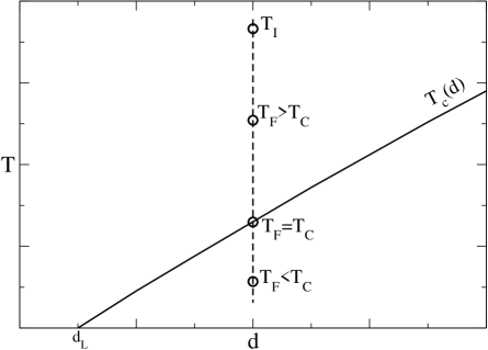
Let us first see where the slow relaxation comes from. The system is supposed to be initially in equilibrium at some temperature $T_{I}$ well above the critical line. For simplicity, take $T_{I}=\infty$ corresponding to an initial state with vanishing correlation length. For a certain value of the dimensionality $d>d_{L}$ (dashed vertical line in Fig.1), the system may be quenched to a final value of the temperature $T_{F}$ greater, equal or lower than the critical temperature $T_{C}$. The relaxation involves the growth of the time dependent correlation length $\xi(t)$ from the initial value $\xi_{I}=0$ to a final value $\xi_{F}>0$, which depends on $T_{F}$. Specifically, $0<\xi_{F}<\infty$ for $T_{F}>T_{C}$, while $\xi_{F}=\infty$ for $T_{F}\leq T_{C}$ if the system is infinite (it will be explained below why $\xi_{F}=\infty$ also when $T_{F}<T_{C}$). Therefore, for $T_{F}>T_{C}$ there is a finite equilibration time $t_{eq}$. For $T_{F}\leq T_{C}$, since $\xi(t)$ typically grows with a power law $\xi(t)\sim t^{1/z}$ [3], the system is always out of equilibrium no matter for how long it is observed. Hence, for phase-ordering systems the mechanism responsible of the slow relaxation in the quench to or to below $T_{C}$ is clear, it is the growth of correlated regions of arbitrarily large size.

The next step is to focus on the features of the relaxation, like aging, which depend on where the system is quenched to on the $(d,T)$ plane. Assuming that the istantaneous quench takes place at $t=0$, aging is manifested through the behavior of two times observables, such as the order parameter autocorrelation function $C(t,t_{w})$ and the autoresponse function $R(t,t_{w})$. The shortest time after the quench $t_{w}\geq 0$ and the longest $t\geq t_{w}$ are conventionally called the waiting time and the observation time. Regarding $t_{w}$ as the age of the system, aging is usually, and quite effectively, meant to say that older systems relax slower and younger ones faster [5]. However, this needs to be explained in more detail, since a rich phenomenology goes under the same heading of aging.

The first relevant feature is the separation of the time scales [2]. This means that when $t_{w}$ is sufficiently large, the range of $\tau=t-t_{w}$ is devided into the short $\tau\ll t_{w}$ and the long $\tau\gg t_{w}$ time separations, and that quite different behaviors are observed in the two regimes. For short $\tau$ the system appears equilibrated. The two time quantities are time translation invariant (TTI) and exhibit the same behavior as if equilibrium at the final temperature of the quench had been reached

$$C(t,t_{w})=C_{eq}(\tau,T_{F}),\;\;\;\;R(t,t_{w})=R_{eq}(\tau,T_{F}).$$ (1)

This is the quasi-equilibrium regime, where the system is ageless. Conversely, for large $\tau$ there is a genuine off-equilibrium behavior obeying a scaling form called simple aging [1, 2]

$$C(t,t_{w})=C_{ag}(t,t_{w})=t_{w}^{-b}h_{C}(t/t_{w})$$ (2)

$$R(t,t_{w})=R_{ag}(t,t_{w})=t_{w}^{-(1+a)}h_{R}(t/t_{w})$$ (3)

where $a,b$ are non negative exponents and $h_{C,R}(t/t_{w})$ are scaling functions. Here, the additional important features are i) that the system does not realize, so to speak, that it is off-equilibrium untill $\tau\sim t_{w}$ and ii) that once the off-equilibrium relaxation gets started, the time scale of the relaxation is fixed by $t_{w}$ itself. Hence, the system ages.

Aging is common to all quenches: above, to and to below $T_{C}$. In the first case, where the equilibration time is finite, for aging to be observable it is necessary that $t_{eq}$ is sufficiently large to allow for both a large $t_{w}$ and $t_{w}\ll t_{eq}$, so that the separation of the time scales is possible. Eventually, when $t_{w}$ hits $t_{eq}$, equilibrium is reached and aging is interrupted.

The phenomenology outlined above suggests the existence of fast and slow degrees of freedom [4, 6, 7]. The separation of the time scales, then, means that, for sufficiently large $t_{w}$, the fast degrees of freedom have already thermalized, while the slow degrees of freedom are still out of equilibrium. This picture is easy to visualize in the case of domain growth. Thinking, for simplicity, of a ferromagnetic system, the fast degrees of freedom are responsible of the thermal fluctuations within ordered domains, while the slow ones are the labels of domains, like the spontaneous magnetization within each domain. The label fluctuates since a given site at different times may belong to different domains. For a given $t_{w}$, the typical size of a domain is $L(t_{w})\sim t_{w}^{1/z}$ and it takes an interval of time $\tau\sim t_{w}$ for a domain wall to sweep the whole domain. Hence, in the short time regime the slow degrees of freedom are frozen and only the fast degrees of freedom contribute to the decay of the two time quantities, yielding the behavior (1). Conversely, in the long time regime, the time evolution is dominated by the motion of domain walls, producing the off-equilibrium behavior of Eqs. (2) and (3).

The picture just outlined is simple and intuitive enough to justify the opinion that aging in domain growth is well understood. Indeed, in section 5.1 an example will be presented where the construction of the fast and slow degrees of freedom can be carried out exactly. However, if the picture works well for the quenches to below $T_{C}$, it cannot be so easily extended also to the quenches to $T_{C}$, where the interpretation in terms of fast and slow degrees of freedom remains less clear. Despite the common features in the phenomenology, a qualitative difference between these two instances of aging, whose origin has not yet been satisfactorily clarified, arises in the way the matching between the stationary and the aging behavior is implemented. In the critical quench stationary and aging behaviors match multiplicatively, while in the quench to below $T_{C}$ the matching is additive.

The existence of these two different realizations of aging poses, among others, quite an interesting problem for what happens in the quench to the special final state located at $(d=d_{L},T_{F}=0)$. Looking at Fig.1, it is evident that such a state can be regarded as a limit state reached either along the critical line or from the ordered region, as $d\rightarrow d_{L}$. However, the two points of view are not equivalent, because the structure of the two times quantities in one case ought to be multiplicative, while in the other additive. As we shall see, the second alternative is the correct one. Nonetheless, in the quench to $(d=d_{L},T_{F}=0)$ there are peculiar features which make it a case apart from both the quenches to and to below $T_{C}$ with $d>d_{L}$. As a matter of fact, the processes listed above can be hierarchically organized in terms of increasing degree of deviation from equilibrium. At the bottom there is the quench to $T_{F}>T_{C}$, where $t_{eq}$ is finite. Immediately above there is the quench to $T_{C}$, where it takes an infinite time to reach equilibrium. Still above there is the quench to $T_{F}<T_{C}$ with $d>d_{L}$, where equilibrium is not reached even in an infinite time. However, this is revealed by the autocorrelation function without appearing in the dynamic susceptibility, which instead behaves as if equilibrium was reached. Lastly, at the top of the hierarchy there is the quench to $(d=d_{L},T_{F}=0)$, where also the dynamic susceptibility displays out of equilibrium behavior over all time scales.

For what concerns the computation of the aging properties, namely the exponents $a,b$ and the scaling functions $h_{C,R}(t,t_{w})$, the systematic expansion methods of field theory, like the $\epsilon$-expansion, can be succesfully used in the quench to $T_{C}$ [8][9]. Perturbative methods, instead, are useless in the quench to below $T_{C}$, where the best theoretical tool for analytical calculations remains the uncontrolled Gaussian auxiliary field (GAF) approximation of the Ohta-Jasnow-Kawasaki type [10], in its various formulations [11]. With methods of this type a good understanding of the autocorrelation function $C(t,t_{w})$ has been achieved [12] (see also the first chapter), while the computation of the autoresponse function $R(t,t_{w})$, in particular of the exponent $a$, remains very much an open problem. For this reason, the investigation of aging in the quench to below $T_{C}$ relies heavily on numerical simultions, although the accurate numerical computation of $R(t,t_{w})$ is a difficult problem of its own [13, 14, 15]. In order to complete the theoretical panorama, the local scale invariance hypothesis [16] must be mentioned. This is a conjecture according to which the response function transforms covariantly under the group of local scale transformations, both in the quenches to and to below $T_{C}$. However, the predictions of this theory are affected by discrepancies with the renormalization group calculations at $T_{C}$ [9] and with the numerical simulations at and below $T_{C}$, which seem to indicate [17][18] that the local scale invariance hypothesis is akin to an approximation of Gaussian nature. Nonetheless, a definite assessment of this approach cannot yet be made, since work is in progress with the proposal of modified versions of the theory [19].

In the following sections an overview of the aging properties in the various quenches mentioned above will be presented, first in general and then through analytical and numerical results for specific models. Preliminary to this discussion is a short summary of the static properties.

2 Statics

In general, order parameter configurations will be denoted by $[\varphi(\vec{x})]$ and the Hamiltonian of the system by ${\cal H}[\varphi(\vec{x})]$. The variable $\varphi$ may be a scalar or a vector and $\vec{x}$ may denote either the points in a continous region or the sites of a lattice. The set of all possible configurations forms the phase space $\Omega$. Symmetries of the system are the groups of transformations of $\Omega$ onto itself, which leave ${\cal H}[\varphi(\vec{x})]$ invariant. The equilibrium state at the temperature $T$ is the Gibbs state

$$P_{G}[\varphi(\vec{x})]={1\over Z}\exp\{-{\cal H}[\varphi(\vec{x})]/T\}$$ (4)

where $Z=\sum_{[\varphi(\vec{x})]}\exp\{-{\cal H}[\varphi(\vec{x})]/T\}$ and the Boltzmann constant is taken $k_{B}=1$. It is evident that $P_{G}[\varphi(\vec{x})]$ shares the symmetries of the Hamiltonian.

The models considered are characterized by the existence of a critical temperature $T_{C}$ and a phase diagram as in Fig.1. For $T\geq T_{C}$ the symmetry is not broken and $P_{G}[\varphi(\vec{x})]$ is a pure state. For $T<T_{C}$ the symmetry is broken and $P_{G}[\varphi(\vec{x})]$ is a mixture

$$P_{G}[\varphi(\vec{x})]=\sum_{\alpha}w_{\alpha}P_{\alpha}[\varphi(\vec{x})]$$ (5)

where the broken symmetry pure states $P_{\alpha}[\varphi(\vec{x})]$ are invariant under a subgroup of the symmetry group of the Hamiltonian, while the weights $w_{\alpha}\geq 0$ satisfy $\sum_{\alpha}w_{\alpha}=1$. In the Gibbs state, due to symmetry, all the weights are equal

$$w_{\alpha}=w,\qquad\forall\;\alpha.$$ (6)

Thus, for example, in the case of the Ising model, where the order parameter configurations are spin configurations $[s_{i}=\pm 1]$ on a lattice, below $T_{C}$ there are two pure states, labeled by $\alpha=\pm$, which transform one into the other under spin inversion

$$P_{+}[s_{i}]=P_{-}[-s_{i}]$$ (7)

and remain invariant under the trivial subgroup of the identity. The Gibbs state is given by

$$P_{G}[s_{i}]=w_{+}P_{+}[s_{i}]+w_{-}P_{-}[s_{i}]$$ (8)

with $w_{+}=w_{-}=w=1/2$. With a vector order parameter and ${\cal H}[\vec{\varphi}(\vec{x})]$ invariant under rotations, the labels of the pure states are the unit vectors $\hat{\alpha}$ in the the order parameter space and each broken symmetry state $P_{\hat{\alpha}}[\vec{\varphi}(\vec{x})]$ is invariant under the subgroup of the rotations around the $\hat{\alpha}$ axis.

2.1 Magnetization

We shall assume throughout, except when it will be explicitely stated otherwise, that all expectation values are space translation invariant. Then, the equilibrium magnetization is given by

$$m_{eq}=\langle\varphi(\vec{x})\rangle_{G}$$ (9)

where $\langle\cdot\rangle_{G}$ denotes averages taken with respect to $P_{G}[\varphi(\vec{x})]$. Since $\varphi(\vec{x})$ is not symmetrical, $m_{eq}$ must vanish for all temperatures. Namely, the existence of the phase transition cannot be detected from the magnetization in the Gibbs state. Below $T_{C}$, using Eqs. (5) and (6)

$$m_{eq}=w\sum_{\alpha}m_{\alpha}=0$$ (10)

where $m_{\alpha}=\langle\varphi(\vec{x})\rangle_{\alpha}\neq 0$ is the spontaneous magnetization in the pure state $P_{\alpha}[\varphi(\vec{x})]$. What vanishes below $T_{C}$ is the sum of all the possible values of the spontaneous magnetization, but separately each contribution is not zero.

2.2 Correlation function

Conversely, the behavior of the order parameter correlation function

$$C_{eq}(\vec{r},T)=\langle\varphi(\vec{x}+\vec{r})\varphi(\vec{x})\rangle_{G}-\langle\varphi(\vec{x}+\vec{r})\rangle_{G}\langle\varphi(\vec{x})\rangle_{G}$$ (11)

allows to detect the existence of the phase transition, even in the symmetrical Gibbs state. From the scaling behavior for $T\geq T_{C}$

$$C_{eq}(\vec{r},T)=r^{-(d-2+\eta)}f_{eq}(r/\xi)$$ (12)

where $\xi$ is the correlation length and $f_{eq}(x)$ is a rapidly vanishing scaling function, follows the clustering property

$$\lim_{r\to\infty}C_{eq}(\vec{r},T)=0.$$ (13)

Instead, for $T<T_{C}$, from Eqs. (11) and (5) follows

$$C_{eq}(\vec{r},T)=\sum_{\alpha}w_{\alpha}C_{\alpha}(\vec{r},T)+q_{eq}$$ (14)

where

$$C_{\alpha}(\vec{r},T)=\langle\varphi(\vec{x}+\vec{r})\varphi(\vec{x})\rangle_{\alpha}-\langle\varphi(\vec{x}+\vec{r})\rangle_{\alpha}\langle\varphi(\vec{x})\rangle_{\alpha}$$ (15)

is the correlation function in the $\alpha$-th broken symmetry state and

$$q_{eq}=\sum_{\alpha}w_{\alpha}m_{\alpha}^{2}-\left[\sum_{\alpha}w_{\alpha}m_{\alpha}\right]^{2}$$ (16)

is the variance of the spontaneous magnetization in the Gibbs state. This quantity in the spin glass context is the Edwards-Anderson order parameter [20]. Since $C_{\alpha}(\vec{r},T)$ and $m_{\alpha}^{2}$ are independent of $\alpha$, it is convenient to introduce the notation $G_{eq}(\vec{r},T)=C_{\alpha}(\vec{r},T)$, $M^{2}=m_{\alpha}^{2}$ and to rewrite

$$C_{eq}(\vec{r},T)=G_{eq}(\vec{r},T)+M^{2}$$ (17)

where $G_{eq}(\vec{r},T)$ has a form similar to (12)

$$G_{eq}(\vec{r},T)=r^{-(d-2+\eta)}g_{eq}(r/\xi).$$ (18)

The appearence of a non zero value of $M^{2}$ upon crossing $T_{C}$

$$\lim_{r\to\infty}C_{eq}(\vec{r},T)=M^{2}\neq 0$$ (19)

signals the occurrence of the phase transition and the breaking of ergodicity [21]. Notice that $C_{eq}(\vec{r},T)$ is a connected correlation function and its decay to a non vanishing value at large distances implies that the correlation length $\xi_{G}$ in the Gibbs state is divergent for $T<T_{C}$, as opposed to $\xi$ in the pure states, which is finite for $T<T_{C}$.

2.3 Splitting of the order parameter

The structure (17) of the correlation function can be viewed as due to the splitting of the order parameter into the sum of two statistically independent contributions

$$\varphi(\vec{x})=\psi(\vec{x})+\sigma$$ (20)

each with zero mean

$$\langle\psi(\vec{x})\rangle=\langle\sigma\rangle=0$$ (21)

and such that

$$G_{eq}(\vec{r},T)=\langle\psi(\vec{x}+\vec{r})\psi(\vec{x})\rangle$$ (22)

$$M^{2}=\langle\sigma^{2}\rangle.$$ (23)

The first contribution represents the thermal fluctuations in any of the pure states and is obtained by shifting the order parameter by its mean

$$\psi(\vec{x})=\varphi(\vec{x})-m_{\alpha}.$$ (24)

This quantity averages to zero by construction and the probability distribution

$$P[\psi(\vec{x})]=P_{\alpha}[\psi(\vec{x})+m_{\alpha}]$$ (25)

is independent of $\alpha$, since the deviations from the mean are equally distributed in all pure states. The second contribution $\sigma$ fluctuates over the possible values of the spontaneous magnetization, taking the values $m_{\alpha}$ with probabilities $P(m_{\alpha})=w_{\alpha}$. Then, from Eqs. (10) and (16) follows

$$\langle\sigma\rangle=0,\qquad M^{2}=\langle\sigma^{2}\rangle.$$ (26)

2.4 Static susceptibility

The introduction of a field $h(\vec{x})$ conjugate to the order parameter modifies the Hamiltonian

$${\cal H}_{h}[\varphi(\vec{x})]={\cal H}[\varphi(\vec{x})]-\sum_{\vec{x}}h(\vec{x})\varphi(\vec{x})$$ (27)

and the corresponding Gibbs state

$$P_{G,h}[\varphi(\vec{x})]={1\over Z_{h}}\exp\{-{\cal H}_{h}[\varphi(\vec{x})]/T\}.$$ (28)

With an $\vec{x}$ dependent external field averages are no more space translation invariant and, if the field is small, the magnetization at the site $\vec{x}$ is given by

$$\langle\varphi(\vec{x})\rangle_{G,h}=\langle\varphi(\vec{x})\rangle_{0}+\int d\vec{y}\;\chi_{st}(\vec{x}-\vec{y},T)h(\vec{y})+{\cal O}(h^{2})$$ (29)

where $\langle\varphi(\vec{x})\rangle_{0}$ is the magnetization in the state

$$P_{0}[\varphi(\vec{x})]=\lim_{h\to 0}P_{G,h}[\varphi(\vec{x})]=\left\{\begin{array}[]{ll}P_{G}[\varphi(\vec{x})],\qquad$for$\qquad T\geq T_{C}\\ P_{\alpha}[\varphi(\vec{x})],\qquad$for$\qquad T<T_{C}\end{array}\right.$$ (30)

and $P_{\alpha}[\varphi(\vec{x})]$ here stands for the particular broken simmetry state selected when the external field is switched off. The site dependent static susceptibility is given by

$$\chi_{st}(\vec{x}-\vec{y},T)=\left.{\delta\langle\varphi(\vec{x})\rangle_{G,h}\over\delta h(\vec{y})}\right|_{h=0}$$ (31)

and making the expansion, up to first order in $h(\vec{x})$, also in the definition

$$\langle\varphi(\vec{x})\rangle_{G,h}=\sum_{[\varphi(\vec{x}^{\prime})]}\varphi(\vec{x})P_{G,h}[\varphi(\vec{x}^{\prime})]$$ (32)

from the comparison with Eq. (29) it is straightforward to derive the fluctuation-response theorem

$$\chi_{st}(\vec{r},T)={1\over T}C_{0}(\vec{r},T)$$ (33)

where $C_{0}(\vec{r},T)$ is the correlation function in the state $P_{0}[\varphi(\vec{x})]$.

3 Dynamics

Let us now examine the time dependent properties in the various quenches described in the introductory section. The order parameter expectation value and correlator in the infinite temperature initial state $P_{G}[\varphi,T_{I}]$ are given by

$$\langle\varphi(\vec{r})\rangle_{I}=0$$ (34)

$$\langle\varphi(\vec{r})\varphi(\vec{r}^{\prime})\rangle_{I}=\Delta\delta(\vec{r}-\vec{r}^{\prime}).$$ (35)

Modelling the dynamics with a Markov stochastic process, the time dependent probality distribution evolves with the master equation

$${\partial\over\partial t}P[\varphi,t]=\sum_{[\varphi^{\prime}]}\Gamma([\varphi]|[\varphi^{\prime}])P[\varphi^{\prime},t]$$ (36)

where $\Gamma([\varphi]|[\varphi^{\prime}])$ is the transition probability per unit time from $[\varphi^{\prime}]$ to $[\varphi]$, satisfying the detailed balance condition with the Gibbs state at the final temperature $T_{F}$

$$\Gamma([\varphi]|[\varphi^{\prime}])P_{G}[\varphi^{\prime},T_{F}]=\Gamma([\varphi^{\prime}]|[\varphi])P_{G}[\varphi,T_{F}].$$ (37)

Therefore, the dynamics preserves the symmetry of the Hamiltonian and, if equilibrium is reached, then necessarily $P[\varphi,t]$ must go over to $P_{G}[\varphi,T_{F}]$. The crucial question, of course, is whether the system equilibrates or not. As anticipated in the Introduction, four qualitatively different relaxation processes arise, depending on the values of $d$ and $T_{F}$

1. quench to $T_{F}>T_{C}$: there is a finite equilibration time $t_{eq}$

2. quench to $T_{F}=T_{C}$: equilibrium is reached in an infinite time

3. quench to $(d>d_{L},T_{F}<T_{C})$: $C(t,t_{w})$ does not equilibrate, while the dynamic susceptibility $\chi(t,t_{w})$ equilibrates

4. quench to $(d=d_{L},T_{F}=0)$: neither $C(t,t_{w})$ nor $\chi(t,t_{w})$ do equilibrate.

The dynamic susceptibility $\chi(t,t_{w})$ will be defined more precisely in section 4 as the zero field cooled susceptibility.

3.1 Equilibration

Since $P[\varphi,t]$ remains symmetrical during the relaxation, no information on the equilibration process can be extracted from the time dependent magnetization, which vanishes throughout $m(t)=\langle\varphi(\vec{r},t)\rangle\equiv 0$. One must turn to the time dependent correlation function

$$C(\vec{r},t,t_{w})=\langle\varphi(\vec{x}+\vec{r},t)\varphi(\vec{x},t_{w})\rangle-\langle\varphi(\vec{x}+\vec{r},t)\rangle\langle\varphi(\vec{x},t_{w})\rangle$$ (38)

where the angular brackets denote the average over the initial condition and the thermal noise. For what is needed in the following it is sufficient to consider the autocorrelation function $C(t,t_{w})=C(\vec{r}=0,t,t_{w})$.

If there exists a finite equilibration time $t_{eq}$, then for $t_{w}>t_{eq}$ the dynamics becomes TTI with

$$C(t,t_{w})=C_{eq}(\tau,T_{F}).$$ (39)

So, if it is not known how large $t_{eq}$ is, or if it exists at all, in order to ascertain whether equilibration has occurred or not, it is necessary to look at the large $t_{w}$ behavior. The $t_{w}\rightarrow\infty$ limit requires to specify also how $t$ is pushed to infinity. This is done by rewriting $C(t,t_{w})$ in terms of the new pairs of variables $(\tau,t_{w})$ and $(x=t/t_{w},t_{w})$

$$C(t,t_{w})=\widetilde{C}(\tau,t_{w})=\widehat{C}(x,t_{w})$$ (40)

and, then, by taking the limit $t_{w}\rightarrow\infty$ while keeping either $\tau$ or $x$ fixed. The short $\tau\ll t_{w}$ and the large $\tau\gg t_{w}$ time separation regimes are explored, respectively, in the first and in the second case. Notice that from $x=\tau/t_{w}+1$ follows that when using the $x$ variable the short time regime gets all compressed into $x=1$. Assuming that the limits exist, one has

$$\lim_{t_{w}\to\infty}\widetilde{C}(\tau,t_{w})=K_{C}(\tau)$$ (41)

and

$$\lim_{t_{w}\to\infty}\widehat{C}(x,t_{w})={\cal C}(x)$$ (42)

which, in general, are two functions not related one to the other. However, if there exists an equilibration time $t_{eq}$ and Eq.(39) holds on all time scales, then $K_{C}(\tau)=C_{eq}(\tau,T_{F})$ and for $t_{w}>t_{eq}$

$$\widehat{C}(x,t_{w})=C_{eq}((x-1)t_{w},T_{F})$$ (43)

which implies the singular limit

$${\cal C}(x)=\left\{\begin{array}[]{ll}C_{eq}(0,T_{F}),\qquad$for$\qquad x=1\\ C_{eq}(\infty,T_{F}),\qquad$for$\qquad x>1.\end{array}\right.$$ (44)

This is a necessary condition for equilibration. To be also a sufficient condition it should hold for all two times observables. As we shall see below it may hold for some, but not for others.

3.2 Generic properties of $C(t,t_{w})$

In the quench to $T_{F}>T_{C}$, since there is a finite equilibration time, Eq. (44) necessarily holds. The interesting cases are those of the quenches to and to below $T_{C}$, where $t_{eq}$ diverges.

In the quench to $T_{C}$, the generic form of $C(t,t_{w})$ displays the multiplicative combination of the stationary and aging contributions [22, 9]

$$C(t,t_{w})=(\tau+t_{0})^{-b_{c}}g_{C}(t/t_{w})$$ (45)

where

$$b_{c}=(d-2+\eta)/z_{c}$$ (46)

$\eta$ is the usual static exponent, $z_{c}$ is the dynamical critical exponent [23] and $t_{0}$ is a microscopic time needed to regularise the equal time autocorrelation function. Taking the short time limit (41) $K_{C}(\tau)$ is found to coincide with the autocorrelation function of equilibrium critical dynamics

$$C_{eq}(\tau,T_{C})=(\tau+t_{0})^{-b_{c}}g_{C}(1)$$ (47)

where $C_{eq}(0,T_{C})=t_{0}^{-b_{c}}g_{C}(1)=\langle\varphi^{2}(\vec{x})\rangle_{G}$. In order to explore the large time regime, Eq. (45) can be rewritten in the simple aging form

$$C(t,t_{w})=t_{w}^{-b_{c}}f_{C}(x,y)$$ (48)

with $y=t_{0}/t_{w}$. The scaling function

$$f_{C}(x,y)=(x-1+y)^{-b_{c}}g_{C}(x)$$ (49)

decreases asymptotically with the power law

$$f_{C}(x,y)=A_{C}x^{-\lambda_{c}/z_{c}}$$ (50)

where $\lambda_{c}$ is the critical autocorrelation exponent [24]. Then, taking the $t_{w}\rightarrow\infty$ limit one finds

$${\cal C}(x)=\left\{\begin{array}[]{ll}t_{0}^{-b_{c}}g_{C}(1),\qquad$for$\qquad x=1\\ 0,\qquad$for$\qquad x>1\end{array}\right.$$ (51)

in agreement with Eq. (44). Therefore, although it is clear that equilibrium is not reached in any finite time, the autocorrelation function behaves as if equilibrium was reached in an infinite time.

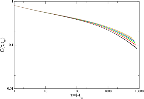
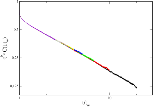
As an illustration, the behavior of $C(t,t_{w})$ in the quench to $T_{C}$ of the $d=2$ kinetic Ising model with Glauber dynamics [25] is displayed in Figs. 2 and 3. In the first one $\widetilde{C}(\tau,t_{w})$ is plotted agains $\tau$ for increasing values of $t_{w}$, showing quite well the separation of the time scales, since the curves collapse in the short time regime and spread out as the large time regime is entered. Furthermore, the collapse improves with increasing $t_{w}$, showing the convergence of $\widetilde{C}(\tau,t_{w})$ toward $C_{eq}(\tau,T_{C})$. The multiplicative structure is demonstrated in Fig.3, where the plot of $\tau^{b_{c}}C(t,t_{w})$ against $x$ for different values of $t_{w}$ shows the collapse of the data as required by Eq. (45), since in the chosen $t_{w}$ range $t_{0}$ is negligible. This plot has been made using $b_{c}=0.115$ obtained from Eq. (46) with $\eta=1/4$ and $z_{c}=2.167$ [26].

Figure 2: $\widetilde{C}(\tau,t_{w})$ vs. $\tau$ in the quench to $T_{C}$ of the $d=2$ kinetic Ising model. $t_{w}$ is incresing by $500$ from $1500$ up to $4000$ (bottom to top). In this and in the following figures times are always in units of Monte Carlo steps.

Figure 3: $\tau^{b_{c}}C(t,t_{w})$ vs. $x=t/t_{w}$ in the quench to $T_{C}$ of the $d=2$ kinetic Ising model and for the same values of $t_{w}$ as in Fig.2. The collapse of the different curves demonstrates the multiplicative structure of Eq.(45).

When the quench is made to $T_{F}<T_{C}$, in the short time regime the $t_{w}\rightarrow\infty$ limit gives, again, the equilibrium behavior

$$K_{C}(\tau)=C_{eq}(\tau,T_{F})=G_{eq}(\tau,T_{F})+M^{2}.$$ (52)

For large time, instead, one finds

$${\cal C}(x)=\left\{\begin{array}[]{ll}C_{eq}(0,T_{F}),\qquad$for$\qquad x=1\\ h_{C}(x),\qquad$for$\qquad x>1\end{array}\right.$$ (53)

where $h_{C}(x)$ is a monotonously decaying function with the limiting behaviors

$$h_{C}(x)=\left\{\begin{array}[]{ll}M^{2},\qquad$for$\qquad x=1\\ x^{-\lambda/z},\qquad$for$\qquad x\gg 1\end{array}\right.$$ (54)

and $\lambda$ is the autocorrelation exponent below $T_{C}$ [28]. Therefore, i) the necessary condition (44) for equilibration is violated and ii) the above result, together with Eq. (52), implies the non commutativity of the limits $t_{w}\rightarrow\infty$ and $t\rightarrow\infty$ with

$$\lim_{\tau\to\infty}\lim_{t_{w}\to\infty}C(\tau+t_{w},t_{w})=M^{2}$$ (55)

and

$$\lim_{t_{w}\to\infty}\lim_{t\to\infty}C(t,t_{w})=0.$$ (56)

This is the phenomenon of weak ergodicity breaking [29], since ergodicity appears broken in the short time regime, but not in that of the large time separations. The behaviors described above are illustrated in Figs. 4 and 5, where $C(t,t_{w})$, computed in the quench to $T_{F}=0.66\;T_{C}$ of the $d=2$ kinetic Ising model, is plotted against $\tau$ and $x$. Both plots highlight the separation of time scales, with the collapse of the data either in the short or in the large time regime, as well as the falling of the curves below the Edwards-Anderson plateau at $M^{2}=0.97$, revealing that the system keeps on decorrelating for arbitrarily large time scales.

Figure 4: $\widetilde{C}(\tau,t_{w})$ vs. $\tau$ in the quench to $T_{F}=0.66\;T_{C}$ of the $d=2$ kinetic Ising model. $t_{w}$ is incresing by $500$ from $2000$ up to $4000$ (bottom to top). The orizontal line indicates the Edwards-Anderson order parameter $M^{2}=0.97$.

Figure 5: $C(t,t_{w})$ vs. $x=t/t_{w}$ in the quench to $T_{F}=0.66\;T_{C}$ of the $d=2$ kinetic Ising model and for the same values of $t_{w}$ as in Fig.4.

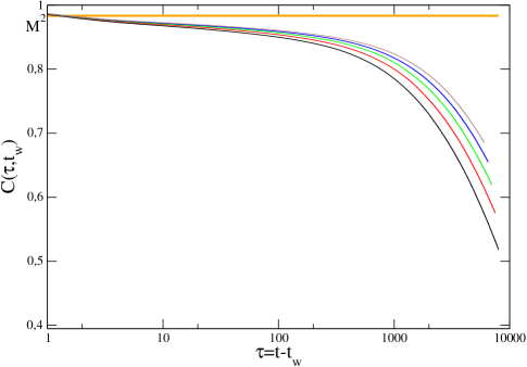
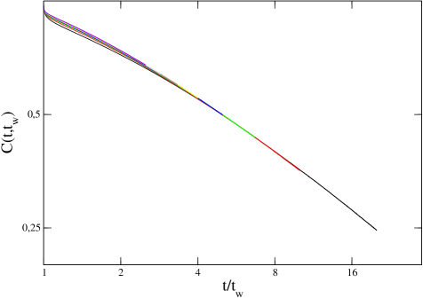
The curve in Fig.5 for $x>3$, where the collapse is good, essentially is a plot of $h_{C}(x)$.

Weak ergodicity breaking is incompatible with the multiplicative form (45). Then, in order to put together the separation of the time scales and weak ergodicity breaking, $C(t,t_{w})$ must have the additive structure

$$C(t,t_{w})=G_{eq}(\tau,T_{F})+C_{ag}(t,t_{w})$$ (57)

where $C_{ag}(t,t_{w})$ obeys the simple aging form (2) with the scaling function $h_{C}(x)$ and $b=0$. Notice that this value of $b$ is of geometrical origin, since it is related through the multitime scaling of Furukawa [27]

$$C_{ag}(\vec{r},t,t_{w})={\cal F}(r/t^{1/z},t/t_{w})$$ (58)

to the well known [3] scaling of the equal time correlation function

$$C_{ag}(\vec{r},t)=F(r/t^{1/z})={\cal F}(r/t^{1/z},1)$$ (59)

which, in turn, is a consequence of the compact nature of the ordered domains. Here $z$ is the phase-ordering growth exponent with the value $z=2$ for dynamics with non conserved order parameter [3].

3.3 Splitting of the order parameter

The additive structure (57) leads, for large time, to the generalization of the splitting (20) of the order parameter into the sum of two time dependent components

$$\varphi(\vec{x},t)=\psi(\vec{x},t)+\sigma(\vec{x},t)$$ (60)

in such a way that the two contributions are still statistically independent, of zero mean and with the respective autocorrelation functions given by

$$\langle\psi(\vec{x},t)\psi(\vec{x},t_{w})\rangle=G_{eq}(\tau,T_{F})$$ (61)

$$\langle\sigma(\vec{x},t)\sigma(\vec{x},t_{w})\rangle=C_{ag}(t,t_{w}).$$ (62)

The variables $\psi(\vec{x},t)$ and $\sigma(\vec{x},t)$ are associated to the fast and slow degrees of freedom [4, 6, 7]. Keeping in mind the domain structure of the configurations, the local ordering variable is defined by

$$\sigma(\vec{x},t)=m_{\alpha(\vec{x},t)}$$ (63)

where $\alpha(\vec{x},t)$ is the value of $\alpha$ selected by the domain to which the site $\vec{x}$ belongs at the time $t$. Hence, $\sigma(\vec{x},t)$ represents the local equilibrium magnetization within domains, while $\psi(\vec{x},t)$ is the field of thermal fluctuations, as in Eq. (20). The off-equilibrium character of the dynamics enters only through the ordering variable $\sigma(\vec{x},t)$. In fact, while $\psi(\vec{x},t)$ executes the equilibrium thermal fluctuations, $\sigma(\vec{x},t)$ can change only if a defect, or an interface, goes by the site $\vec{x}$ at the time $t$. In other words, the evolution of $\sigma(\vec{x},t)$ is strictly related to the existence of defects in the system, which is precisely what keeps the system out of equilibrium. As we shall see in section 5.1, in the case of the large $N$ model the construction (60) can be carried out exactly.

4 Linear response function

As previously stated, the quench of phase-ordering systems offers the full spectrum of off-equilibrium phenomena, with increasing degree of deviation from equilibrium as $T_{F}$ is lowered from above to below $T_{C}$. The survey of aging, so far, has been conducted using the order parameter autocorrelation function as a probe. However, once the basic features of the phenomena involved have been brought into focus, in order to carry out a more refined analysis and to make progress in the characterization of the deviation from equilibrium, it is indispensable to look jointly at the autocorrelation and autoresponse function. In particular, the deviations from the fluctuation-dissipation theorem (FDT) have proven to be a most effective tool of investigation [1, 2]. This approach to the study of out of equilibrium dynamics has been pionereed by Cugliandolo and Kurchan in their groundbreaking work on the mean field models of the spin glass [30].

Let us begin by defining the time dependent linear response function. If a small space and time dependent external field $h(\vec{x},t)$ is switched on in the time interval $(t_{1},t_{2})$ after the quench, then the magnetization at the time $t\geq t_{2}$ is given by

$$\langle\varphi(\vec{x},t)\rangle_{h}=\langle\varphi(\vec{x},t)\rangle+\int d\vec{y}\;\int_{t_{1}}^{t_{2}}dt^{\prime}\;R(\vec{x}-\vec{y},t,t^{\prime})h(\vec{y},t^{\prime})+{\cal O}(h^{2})$$ (64)

where $\langle\varphi(\vec{x},t)\rangle$ is the magnetization in the absence of the field and

$$R(\vec{x}-\vec{y},t,t_{w})={\left.\delta\langle\varphi(\vec{x},t)\rangle_{h}\over\delta h(\vec{y},t_{w})\right|_{h=0}}$$ (65)

is the space and time dependent linear response function. The autoresponse function $R(t,t_{w})$ is obtained taking $\vec{x}=\vec{y}$.

With a time independent external field, Eq. (64) takes the form

$$\langle\varphi(\vec{x},t)\rangle_{h}=\langle\varphi(\vec{x},t)\rangle+\int d\vec{y}\;\zeta(\vec{x}-\vec{y},t,t_{1},t_{2})h(\vec{y})+{\cal O}(h^{2})$$ (66)

where

$$\zeta(\vec{r},t,t_{2},t_{1})=\int_{t_{1}}^{t_{2}}dt^{\prime}R(\vec{r},t,t^{\prime})$$ (67)

is the integrated linear response function. Particular cases, frequently encountered in the literature, are those of the thermoremanent magnetization (TRM) corresponding to the protocol $t_{1}=0$, $t_{2}=t_{w}$

$$\rho(\vec{r},t,t_{w})=\zeta(\vec{r},t,t_{w},0)$$ (68)

and of the zero field cooled (ZFC) susceptibility corresponding to $t_{1}=t_{w}$, $t_{2}=t$

$$\chi(\vec{r},t,t_{w})=\zeta(\vec{r},t,t,t_{w}).$$ (69)

4.1 Fluctuation-dissipation theorem (FDT)

For convenience, let us briefly derive the FDT. Assuming that the small external field has been applied from a time so distant in the past that equilibrium in the field is established at the time $t_{w}$ and that it is switched off for $t>t_{w}$, the magnetization is given by

$$\langle\varphi(\vec{x},t)\rangle_{h}=\sum_{[\varphi],[\varphi^{\prime}]}\varphi(\vec{x})Q([\varphi,t]|[\varphi^{\prime},t_{w}])P_{G,h}[\varphi^{\prime}]$$ (70)

where $Q([\varphi,t]|[\varphi^{\prime},t_{w}])$ is the conditional probability in the absence of the field, since $t>t_{w}$. Recalling that $P_{G,h}[\varphi]$ is given by Eqs. (27) and (28) and expanding up to first order in the field, one finds

$$\langle\varphi(\vec{x},t)\rangle_{h}=\langle\varphi(\vec{x},t)\rangle+{1\over T_{F}}\int d\vec{y}\;C_{0}(\vec{x}-\vec{y},t-t_{w},T_{F})h(\vec{y})$$ (71)

where $C_{0}(\vec{x}-\vec{y},t-t_{w},T_{F})$ is the equilibrium, unperturbed correlation function in the stationary state (30). Hence, comparing with Eq. (66)

$${1\over T_{F}}C_{0}(\vec{r},t-t_{w},T_{F})=\int_{-\infty}^{t_{w}}dt^{\prime}R(\vec{r},t,t^{\prime})$$ (72)

and differentiating with respect to $t_{w}$ the FDT is obtained

$$R_{eq}(\vec{r},\tau,T_{F})=-{1\over T_{F}}{\partial\over\partial\tau}C_{0}(\vec{r},\tau,T_{F})$$ (73)

where $R_{eq}(\vec{r},\tau,T_{F})$ is the equilibrium response function. From this, it is straightforward to derive the integrated form of the FDT in terms of the equilibrium ZFC susceptibility

$$\chi_{eq}(\vec{r},\tau,T_{F})={1\over T_{F}}[C_{0}(\vec{r},T_{F})-C_{0}(\vec{r},\tau,T_{F})]$$ (74)

and using $\lim_{\tau\to\infty}C_{0}(\vec{r},\tau,T_{F})=0$, this gives the identification, via Eq. (33), of the large time limit of the equilibrium ZFC susceptibility with the static susceptibility

$$\lim_{\tau\to\infty}\chi_{eq}(\vec{r},\tau,T_{F})=\chi_{st}(\vec{r},T_{F}).$$ (75)

4.2 Generic properties of $R(t,t_{w})$

Before exploring the deviations from the FDT when the system is not in equilibrium, it is convenient to go over the generic properties of $R(t,t_{w})$, as it has been done for $C(t,t_{w})$ in section 3.2. Apart for the few cases where analytical results are available, $R(t,t_{w})$ is less known than $C(t,t_{w})$, since it is much more difficult to measure numerically. Actually, untill very recently, $R(t,t_{w})$ was numerically accessible only indirectly through the measurement of the integrated response functions. This situation has partially changed after the introduction of new and more efficient algorithms [13, 14, 15]. In any case, whenever TTI holds, like in equilibrium or in the short time sector, the task is easier since the form of $R(t,t_{w})$ is related to that of $C(t,t_{w})$ via the FDT. When TTI does not hold, scaling arguments will be used.

In the quench to $T_{C}$, the analogue of the multiplicative form (45) reads

$$R(t,t_{w})=(\tau+t_{0})^{-(1+a_{c})}g_{R}(t/t_{w})$$ (76)

whose short time limit $K_{R}(\tau)$ coincides with the equilibrium response function

$$R_{eq}(\tau,T_{C})=(\tau+t_{0})^{-(1+a_{c})}g_{R}(1)$$ (77)

after requiring to be related to $C_{eq}(\tau,T_{C})$ by the FDT. This yields the constraints

$$a_{c}=b_{c}$$ (78)

and

$$T_{C}g_{R}(1)=b_{c}g_{C}(1).$$ (79)

Switching to the $(x,t_{w})$ variables, $R(t,t_{w})$ is rewritten in the simple aging form

$$R(t,t_{w})=t_{w}^{-(1+a_{c})}f_{R}(x,y)$$ (80)

where the scaling function

$$f_{R}(x,y)=(x-1+y)^{-(1+a_{c})}g_{R}(x)$$ (81)

for large $x$ decreases with the same power law as $f_{C}(x,y)$ [8]

$$f_{R}(x,y)=A_{R}x^{-\lambda_{c}/z_{c}}.$$ (82)

Then, taking the $t_{w}\rightarrow\infty$ limit, the analogue of Eq. (51) is obtained

$${\cal R}(x)=\left\{\begin{array}[]{ll}t_{0}^{-(1+b_{c})}g_{R}(1),\qquad$for$\qquad x=1\\ 0,\qquad$for$\qquad x>1\end{array}\right.$$ (83)

which satisfies the necessary condition for equilibration

$${\cal R}(x)=\left\{\begin{array}[]{ll}R_{eq}(0,T_{F}),\qquad$for$\qquad x=1\\ R_{eq}(\infty,T_{F}),\qquad$for$\qquad x>1\end{array}\right.$$ (84)

in the same way as the autocorrelation function.

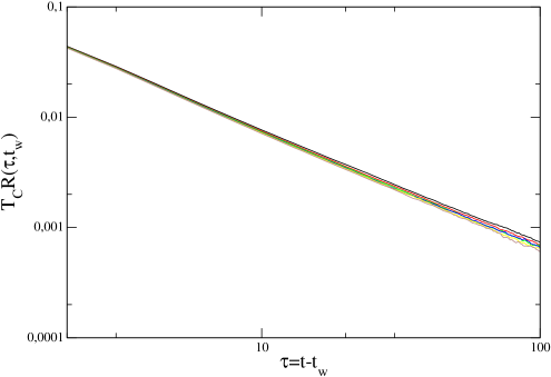
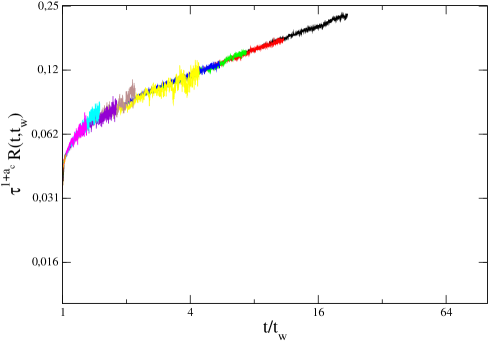
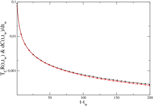
The above behavior is well illustrated by the data for $R(t,t_{w})$, obtained with the algorithm of Ref.[14] in the quench to $T_{C}$ of the $d=2$ kinetic Ising model, along the same line of what has been already done for $C(t,t_{w})$. In Fig.6 $R(t,t_{w})$ is plotted agains $\tau$, displaying, as in Fig.2, the separation of the time scales, with the collapse and the spread of the curves in the short and in the large time regimes, respectively. The collapse of the curves in Fig.7, obtained by plotting $\tau^{1+a_{c}}R(t,t_{w})$ against $x$, demonstrates, as in Fig.3, the multiplicative structure (76). The validity of the FDT in the short time regime is illustrated in Fig.8.

Figure 6: $T_{C}R(\tau,t_{w})$ vs. $\tau$ in the quench to $T_{C}$ of the $d=2$ kinetic Ising model. $t_{w}$ is incresing by $500$ from $1500$ up to $4000$ (bottom to top).

Figure 7: $\tau^{1+a_{c}}R(t,t_{w})$ vs. $x=t/t_{w}$ in the quench to $T_{C}$ of the $d=2$ kinetic Ising model and for the same values of $t_{w}$ as in Fig.6. The collapse of the different curves demonstrates the multiplicative structure of Eq.(76).

Figure 8: Plot of $T_{C}R(t,t_{w})$ and $\partial C(t,t_{w})/\partial t_{w}$ in the quench to $T_{C}$ of the $d=2$ kinetic Ising model, for $t_{w}=1000$. The superposition of the curves for $\tau\ll t_{w}$ demonstrates the validity of the FDT in the short time region.

In the quench to below $T_{C}$, the additivity of $C(t,t_{w})$ induces the corresponding structure in the response function

$$R(t,t_{w})=R_{eq}(\tau,T_{F})+R_{ag}(t,t_{w})$$ (85)

in the following way: the stationary response of the fast degrees of freedom $R_{eq}(\tau,T_{F})$ is defined by requiring the FDT to hold in the short time regime

$$R_{eq}(\tau,T_{F})=-{1\over T_{F}}{\partial\over\partial\tau}G_{eq}(\tau,T_{F})$$ (86)

where $G_{eq}(\tau,T_{F})$ is the stationary contribution entering Eq. (57). The aging component associated to the slow degrees of freedom remains defined, thereafter, by Eq. (85) as the difference $R_{ag}(t,t_{w})=R(t,t_{w})-R_{eq}(\tau,T_{F})$ and obeys the simple aging form (3) where the scaling function decays asymptotically with the same power law as $h_{C}(x)$ [22]

$$h_{R}(x)\sim x^{-\lambda/z}.$$ (87)

Since in the short time regime the FDT must be satisfied also by the full $R(t,t_{w})$, this implies that $R_{ag}(t,t_{w})$ vanishes for short times. Conversely, since $R_{eq}(\tau,T_{F})$ typically is a rapidly decaying function, in the large time regime only $R_{ag}(t,t_{w})$ survives. The behavior of $R(x,t_{w})$ for large $t_{w}$, then, is given by

$$R(x,t_{w})=\left\{\begin{array}[]{ll}R_{eq}(0,T_{F})\qquad$for$\qquad x=1\\ t_{w}^{-(1+a)}h_{R}(x)\qquad$for$\qquad x>1.\end{array}\right.$$ (88)

From this it is easy to see that, for $d>d_{L}$, the condition (84) is satisfied, after taking into account that $a>0$ (as it will be explained shortly) and that $R_{eq}(\infty,T_{F})=0$. Therefore, contrary to what happens with the autocorrelation function, the large $t_{w}$ behavior of $R(t,t_{w})$ does not reveal that the system remains out of equilibrium in the large time regime.

For what concerns the exponent $a$, there is a major difference with respect to the case of the quench to $T_{C}$. Since the FDT in Eq. (86) relates only the stationary components $G_{eq}(\tau,T_{F})$ and $R_{eq}(\tau,T_{F})$, there is no more any constraint relating $a$ to $b$, contrary to what happened in the critical quench where the equality (78) was enforced by the multiplicative structure. In other words, in the quench to below $T_{C}$ the value of $a$ is decoupled from that of $b$ and, as mentioned in the Introduction, the determination of this exponent is a difficult and challenging problem, which will be discussed at the end of the chapter. In any case, although the actual value of $a$ is, to some extent, a debated issue, yet there is general consensus on the statement $a>0$ for $d>d_{L}$. The case of $d=d_{L}$ stands apart and will be discussed in section 4.6.

4.3 ZFC susceptibility below $T_{C}$

It is clear that the additive structure of the response function generates the analogous form of the ZFC susceptibility

$$\chi(t,t_{w})=\chi_{eq}(\tau,T_{F})+\chi_{ag}(t,t_{w})$$ (89)

where the stationary component satisfies, by construction, the equilibrium FDT (74). Inserting the scaling form (3) of $R_{ag}$ in the definition of the aging component

$$\chi_{ag}(t,t_{w})=\int_{t_{w}}^{t}dt^{\prime}R_{ag}(t,t^{\prime})$$ (90)

one finds

$$\chi_{ag}(t,t_{w})=t_{w}^{-a}h_{\chi}(x,y)$$ (91)

where

$$h_{\chi}(x,y)=x^{-a}{\cal I}(x,y)$$ (92)

and

$${\cal I}(x,y)=\int_{1/x}^{1}dz\;z^{-(1+a)}h_{R}(z^{-1},z^{-1}y/x).$$ (93)

Here, we make a first observation which turns out to be quite important in general, when the data for $\chi_{ag}$ from the simulations are used to measure the exponent $a$ [31]. If one seeks to determine $a$ from Eq. (91) by looking at the behavior of $\chi_{ag}$ as $t_{w}$ is varied and $x$ is kept fixed, one must be aware that the $t_{w}$ dependence coming from $y=t_{0}/t_{w}$ may play a role. In other words, $t_{0}$ may act as a dangerous irrelevant variable through a mechanism quite similar to the one causing the breakdown of hyperscaling in static critical phenomena above the upper critical dimensionality $d_{U}$ [32]. In those cases where analytical calculations can be carried out with arbitrary $d$ [7, 33, 34] there exists a value $d^{*}$ of the dimensionality such that the limit for $y\rightarrow 0$ of the integral ${\cal I}(x,y)$ is finite for $d<d^{*}$, while for $d>d^{*}$ there is a singularity of the type

$${\cal I}(x,y)=(y/x)^{-c}\;\widehat{{\cal I}}(x)$$ (94)

with $c>0$, which becomes logarithmic $(c=0)$ for $d=d^{*}$. Hence, $d^{*}$ plays the same role as $d_{U}$ in critical phenomena, but it is clearly unrelated to $d_{U}$. The assumption is that this is a generic feature of the relaxation to below $T_{C}$. Then, Eq. (91) can be rewritten as

$$\chi_{ag}(t,t_{w})=t_{w}^{-a_{\chi}}\widehat{h}_{\chi}(x)$$ (95)

with

$$a_{\chi}=\left\{\begin{array}[]{ll}a,\qquad$for$\qquad d<d^{*}\\ a,\qquad$with log corrections for$\qquad d=d^{*}\\ a-c,\qquad$for$\qquad d>d^{*}\end{array}\right.$$ (96)

and for large $x$

$$\widehat{h}_{\chi}(x)\sim x^{-a_{\chi}}$$ (97)

which, in turn, implies

$$\chi_{ag}(t,t_{w})\sim t^{-a_{\chi}}$$ (98)

for large $t$. The analogy with the breaking of hyperscaling is quite close since, as we shall see, there is a dependence on $d$ of $a_{\chi}$ for $d<d^{*}$, which disappears for $d>d^{*}$.

The second observation concerns the value of $a_{\chi}$ and the asymptotic behavior of $\chi(t,t_{w})$. From Eq. (89) follows

$$\lim_{t\to\infty}\chi(t,t_{w})=\lim_{\tau\to\infty}\chi_{eq}(\tau,T_{F})+\lim_{t\to\infty}\chi_{ag}(t,t_{w})$$ (99)

and, recalling Eqs. (75) and (98), this gives

$$\lim_{t\to\infty}\chi(t,t_{w})=\chi_{st}(T_{F})+\chi^{*}$$ (100)

with

$$\chi^{*}=\left\{\begin{array}[]{ll}0\qquad$for$\qquad a_{\chi}>0\\ \lim_{x\to\infty}\widehat{h}_{\chi}(x)\qquad$for$\qquad a_{\chi}=0.\end{array}\right.$$ (101)

Hence, the ZFC susceptibility reaches the equilibrium value for $a_{\chi}>0$, but not for $a_{\chi}=0$. In other words, for $a_{\chi}>0$ the contribution of the slow degrees of freedom disappears asymptotically, while for $a_{\chi}=0$ there remains an extra contribution $\chi^{*}$ on top of the equilibrium one. This is a very interesting phenomenon. Rewriting Eq. (33) as $T_{F}\chi_{st}(T_{F})=C_{eq}(0,T_{F})-M^{2}$ and recalling that $M^{2}$ plays the role of the Edwards-Anderson order parameter, there is a formal similarity with what happens in the mean-field theory of spin glasses, where the large time limit of the ZFC susceptibility can be written [35] exactly as in Eq. (100). The substantial difference is that in the spin glass case $\chi^{*}$ is an equilibrium quantity, whose appearence is due to replica simmetry breaking [20]. As a matter of fact, the observation of $\chi^{*}>0$ in the simulations of finite dimensional spin glasses is taken as evidence of replica simmetry breaking [36]. Here, instead, $\chi^{*}$ is the difference between the large time limit of the ZFC susceptibility and the same quantity computed from equilibrium statistical mechanics. It is a quantity of purely dynamical origin which appears, as we shall see, in the quench to $(d_{L},T_{F}=0)$ revealing the strong out of equilibrium nature of the relaxation.

4.4 Fluctuation-dissipation ratio (FDR)

If the system is not in equilibrium the FDT does not hold and the violation of the theorem can be used as a measure of the deviation from equilibrium. This idea was implemented by Cugliandolo and Kurchan [30] through the introduction of the FDR

$$X(t,t_{w})={T_{F}R(t,t_{w})\over\partial_{t_{w}}C(t,t_{w})}$$ (102)

which satisfies $X(t,t_{w})\equiv 1$ in equilibrium and $X(t,t_{w})\neq 1$ off-equilibrium. Formally, the FDR allows to define the temperature-like quantity

$$T_{eff}(t,t_{w})={T_{F}\over X(t,t_{w})}$$ (103)

whose interpretation as an effective temperature, however, requires some care [37].

As we have seen, the characterization of systems which remain out of equilibrium for arbitrary long times requires the exploration of the various asymptotic regimes reached as $t_{w}\rightarrow\infty$. An efficient way of doing this is through the reparametrization of the time $t$ in terms of the autocorrelation function. For fixed $t_{w}$, $C(t,t_{w})$ is a monotonously decreasing function of $t$. Hence, inverting with respect to $t$, the function $\widehat{X}(C,t_{w})=X(t(C,t_{w}),t_{w})$ is obtained, whose limit for fixed $C$

$$\lim_{t_{w}\to\infty}\widehat{X}(C,t_{w})={\cal X}(C)$$ (104)

defines the limit FDR in the time sector characterized by the chosen value of $C$ and the associated effective temperature is given by

$${\cal T}(C)={T_{F}\over{\cal X}(C)}.$$ (105)

The correspondence between values of $C$ and the short and long time regimes will be clarified below.

Inserting $X(t,t_{w})$ into the definition (69) of the ZFC susceptibility

$$T_{F}\chi(t,t_{w})=\int_{t_{w}}^{t}dt^{\prime}\;\widehat{X}(C(t,t^{\prime}),t^{\prime}){\partial\over\partial t^{\prime}}C(t,t^{\prime})$$ (106)

and for values of $t_{w}$ so large that Eq. (104) can be used under the integral, the parametric representation of $\chi$ is obtained

$$T_{F}\widehat{\chi}(C(t,t_{w}))=\int_{C(t,t_{w})}^{C(t,t)}dC^{\prime}\;{\cal X}(C^{\prime}).$$ (107)

Differentiating with respect to $C$ this gives

$$-T_{F}{d\widehat{\chi}(C)\over dC}={\cal X}(C)$$ (108)

which relates the limit FDR to the slope of $\widehat{\chi}(C)$. This is the most commonly used way of estimating the FDR, due to the relative ease of computing $\widehat{\chi}(C)$ numerically. Notice that the integrated form (74) of the FDT is recovered from Eq. (107) when ${\cal X}(C)\equiv 1$. In that case the plot of $T_{F}\widehat{\chi}(C)$ is a straight line with slope $-1$, the so called trivial plot, which is the hallmark of equilibrium. Off-equilibrium behavior is conveniently detected through the deviations from the trivial plot.

4.5 Parametric plots

The shape of the parametric plots (Fig.9) can be derived from general considerations. In the quench to above $T_{C}$ the system equilibrates in a finite time and it is straightforward to obtain

$${\cal X}(C)\equiv 1$$ (109)

since $X(t,t_{w})\equiv 1$ for $t_{w}>t_{eq}$. In the case of the critical quench the outcome is almost the same, but the derivation is less straightforward. From Eqs. (48,78,80) one finds

$$X(t,t_{w})=F(x,y)$$ (110)

where

$$F(x,y)=-T_{C}{f_{R}(x,y)\over f_{\partial C}(x,y)}$$ (111)

and

$$f_{\partial C}(x,y)=b_{c}f_{C}(x,y)+\left[x{\partial\over\partial x}f_{C}(x,y)+y{\partial\over\partial y}f_{C}(x,y)\right].$$ (112)

Inverting with respect to $x$ the form (51) of the autocorrelation function

$$x(C)=\left\{\begin{array}[]{ll}\infty,\qquad$for$\qquad C=0\\ 1,\qquad$for$\qquad 0<C\leq C_{eq}(0,T_{C})\end{array}\right.$$ (113)

and inserting into Eq. (110), the limit FDR is obtained

$${\cal X}(C)=\left\{\begin{array}[]{ll}{\cal X}_{\infty},\qquad$for$\qquad C=0\\ 1,\qquad$for$\qquad 0<C\leq C_{eq}(0,T_{C})\end{array}\right.$$ (114)

where

$${\cal X}_{\infty}=\lim_{y\to 0}\lim_{x\to\infty}F(x,y)={T_{C}A_{R}\over A_{C}(\lambda/z_{c}-b_{c})}$$ (115)

is a new universal quantity characteristic of the critical relaxation [22, 38]. The second line of (114) comes from $F(1,0)=T_{C}g_{R}(1)/b_{c}g_{C}(1)$, together with the FDT requirement (79). The above result illustrates quite well the usefulness of the FDR and of the parametric plot in the precise characterization of the off-equilibrium relaxation. Eq. (113) shows that in the critical quench all values of $C>0$ correspond to the short time regime, while the large time corresponds to $C=0$ and in the latter regime the system remains off-equilibrium since, in general, ${\cal X}_{\infty}<1$ (center panel of Fig.9).

In the quench to below $T_{C}$, from the additive structures of $C$ and $R$ follows

$$X(t,t_{w}) = T_{F}\left[{R_{eq}(\tau,T_{F})\over\partial_{t_{w}}G_{eq}(\tau,T_{F})+\partial_{t_{w}}C_{ag}(t,t_{w})}\right.$$

$$+ \left.{R_{ag}(t,t_{w})\over\partial_{t_{w}}G_{eq}(\tau,T_{F})+\partial_{t_{w}}C_{ag}(t,t_{w})}\right].$$

Recalling that $R_{eq}$ and $R_{ag}$ are not simultaneously different from zero when $t_{w}$ is large, the first term in the brackets contributes in the short time regime and the second one in the large time regime, yielding

$$X(t,t_{w})=\left\{\begin{array}[]{ll}1\qquad$for$\qquad x=1\\ t_{w}^{-a}H(x,y)\qquad$for$\qquad x>1\end{array}\right.$$ (117)

where

$$H(x,y)=-T_{F}{h_{R}(x,y)\over h_{\partial C}(x,y)}$$ (118)

with

$$h_{\partial C}(x,y)=\left[x{\partial\over\partial x}h_{C}(x,y)+y{\partial\over\partial y}h_{C}(x,y)\right].$$ (119)

Again, inverting with respect to $x$ the autocorrelation function (53)

$$x(C)=\left\{\begin{array}[]{ll}h_{C}^{-1}(C),\qquad$for$\qquad C<M^{2}\\ 1,\qquad$for$\qquad M^{2}\leq C\leq C_{eq}(0,T_{F})\end{array}\right.$$ (120)

and inserting into (117) one finds

$$X(C,t_{w})=\left\{\begin{array}[]{ll}t_{w}^{-a}H(h_{C}^{-1}(C),y),\qquad$for$\qquad C<M^{2}\\ 1,\qquad$for$\qquad M^{2}\leq C\leq C_{eq}(0,T_{F})\end{array}\right.$$ (121)

whose $t_{w}\rightarrow\infty$ limit for $d>d_{L}$, that is when $a>0$, gives

$${\cal X}(C)=\left\{\begin{array}[]{ll}0\qquad$for$\qquad C<M^{2}\\ 1\qquad$for$\qquad M^{2}\leq C\leq C_{eq}(0,T_{F}).\end{array}\right.$$ (122)

Here, the off-equilibrium character of the relaxation is expanded and enhanced, with respect to the critical quench (left panel of Fig.9). The quasi equilibrium in the short time regime is limited to values of $C$ above the Edwards-Anderson plateau and the deviation from equilibrium for large time is more pronounced, since the FDR vanishes.

The corresponding parametric representations of the ZFC susceptibility are easily obtained (Fig.10), by integration. In the quenches to above and to $T_{C}$, both Eqs. (109) and (114) yield the same trivial plot

$$T_{C}\hat{\chi}(C)=C_{eq}(0,T_{C})-C.$$ (123)

Notice that if one goes back differentiating with respect to $C$, one finds identically ${\cal X}(C)=1$ for all values of $C$, above and at $T_{C}$. This clarifies that in order to uncover the existence of the non trivial FDR ${\cal X}_{\infty}$, the order of the limits in Eq. (115) is crucial. In the quench to below $T_{C}$, instead, the departure from the trivial behavior is most evident

$$T_{F}\hat{\chi}(C)=\left\{\begin{array}[]{ll}C_{eq}(0,T_{F})-M^{2}\qquad$for$\qquad C<M^{2}\\ C_{eq}(0,T_{F})-C\qquad$for$\qquad M^{2}\leq C\leq C_{eq}(0,T_{F})\end{array}\right.$$ (124)

since the plot is flat for $C<M^{2}$. This plot shows at glance that the susceptibility equilibrates, while the autocorrelation function does not. The rise from zero to $C_{eq}(0,T_{F})-M^{2}$ in the left panel of Fig.10 shows the saturation of $\widehat{\chi}(C)$ to the static value $T_{F}\chi_{st}(T_{F})=G_{eq}(0,T_{F})$ as $C$ decays to the Edwards-Anderson plateau. For larger times the susceptibility remains fixed at the equilibrium value in the flat portion of the plot, while $C$ falls below the plateau, according to the weak ergodicity breaking scenario.

Figure 9: The limit FDR ${\cal X}(C)$.

Figure 10: Parametric plots of the ZFC susceptibility $\hat{\chi}(C)$ with $C_{eq}(0,T_{F})=1$

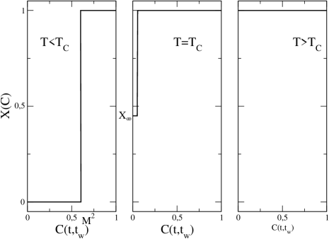
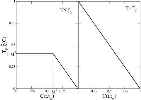
The results above described are universal, since all the non universal features of $F(x,y)$ and $H(x,y)$ have been eliminated in the $t_{w}\rightarrow\infty$ limit. Therefore, in all the quenches to $T_{C}$ the parametric plots of ${\cal X}(C)$ and $T_{C}\hat{\chi}(C)$ are trivial, except for the value of ${\cal X}_{\infty}$, and in all quenches to below $T_{C}$ the deviation from the trivial plot takes the form of the flat behavior below the Edwards-Anderson plateau. For the parametric plots in the quench to $(d_{L},T_{F})$ it is not possible to make statements of such generality. Comments will be made in the next section.

Finally, few words about the effective temperature. From Eqs. (105) and (109) follows that ${\cal T}(C)$ coincides with the temperature of the thermal bath $T_{F}$, when the plot of $T_{F}\hat{\chi}(C)$ is trivial. For $T_{F}>T_{C}$ this happens for all values of $C$. For $T_{F}=T_{C}$ this happens for all values of $C$, except $C=0$, where ${\cal T}(0)=T_{F}/{\cal X}_{\infty}>T_{F}$ and, finally, for $T_{F}<T_{C}$

$${\cal T}(C)=\left\{\begin{array}[]{ll}\infty\qquad$for$\qquad C<M^{2}\\ T_{F}\qquad$for$\qquad M^{2}\leq C\leq C_{eq}(0,T_{F}).\end{array}\right.$$ (125)

The latter result is suggestive that in the quench to below $T_{C}$, while the fast degrees of freedom thermalize, the slow ones do not interact at all with the thermal bath and keep on remaining to the temperature $T_{I}$ of the initial condition.

4.6 A special case: the quench to $(d_{L},T_{F}=0)$

An interesting and non trivial situation arises if the system is at the lower critical dimensionality $d_{L}$ and the quench is made at $T_{F}=0$. As anticipated in the Introduction, this process can be regarded as the limit for $d\rightarrow d_{L}$ either of critical quenches or of quenches made to below $T_{C}$. In the first case from Eq. (114)

$${\cal X}(C)=\left\{\begin{array}[]{ll}0,\qquad$for$\qquad C=0\\ 1,\qquad$for$\qquad 0<C\leq C_{eq}(0,T_{C})\end{array}\right.$$ (126)

since ${\cal X}_{\infty}=0$, while in the second case from Eq. (122)

$${\cal X}(C)=\left\{\begin{array}[]{ll}0\qquad$for$\qquad C<C_{eq}(0,T_{F})\\ 1\qquad$for$\qquad C=C_{eq}(0,T_{F})\end{array}\right.$$ (127)

since $C_{eq}(0,T_{F})=M^{2}$ at $T_{F}=0$. Hence, two very different results are obtained and there is the problem of which is the correct one. What can be stated on general grounds is that the quench to $(d_{L},T_{F}=0)$ is akin to a quenche to below $T_{C}$, since $G_{eq}(\tau,T_{F})\equiv 0$ at $T_{F}=0$ and, therefore, $C(t,t_{w})$ must necessarily have the additive structure, otherwise would vanish identically. Hence, Eq. (126) can be discarded. However, from the analytical [7, 39, 40, 34] and numerical [41, 42] evidence accumulated so far, ${\cal X}(C)$ does not obey Eq. (127) either. Rather, ${\cal X}(C)$ appears to be a non-trivial and non-universal smooth function. Such a behavior is compatible with Eq. (121) if $a=0$, which yields the smooth behavior

$${\cal X}(C)=H(h_{C}^{-1}(C),0)$$ (128)

preserving all the non-universal features of $h_{C}(x,0)$ and $H(x,0)$. Therefore, in the quench to $(d_{L},T_{F}=0)$, although belonging to the class of the quenches to below $T_{C}$, there are peculiarities induced by the vanishing of the exponent $a$.

5 Models

The general concepts introduced in the previous sections will now be illustrated through analytical and numerical results for specific models, limiting the discussion to the case of non conserved order parameter. The models considered are

• the Ising model with the Hamiltonian

  $${\cal H}[s_{i}]=J\sum_{<ij>}s_{i}s_{j}$$ (129)

  where the sum runs over the pairs $<ij>$ of the nearest neighbors spins with the ferromagnetic coupling $J<0$. The time evolution with Glauber single spin flip dynamics [44] is governed by the master equation

  $${\partial\over\partial t}P([s],t)=\sum_{i}\left\{w(-s_{i})P([R_{i}s],t)-w(s_{i})P([s],t)\right\}$$ (130)

  where $P([s],t)$ is the probability of realization of the spin configuration $[s]$ at the time $t$ and $[R_{i}s]$ is the configuration with the $i$-th spin reversed,

  $$w(s_{i})={1\over 2\tau_{0}}[1-s_{i}\tanh(E_{i}/T)]$$ (131)

  is the transition rate from $[s]$ to $[R_{i}s]$, $\tau_{0}$ is a constant and $E_{i}=h_{i}+J\sum_{j\in<i>}s_{j}$ is the sum of the external and the local field on the spin $s_{i}$, due to its nearest neighbors.

• the continous Ginzburg-Landau-Wilson (GLW) model with the Hamiltonian

  $${\cal H}[\vec{\phi}(\vec{x})]=\int_{V}d\vec{x}\;\left[{1\over 2}(\nabla\vec{\phi})^{2}+{\mu\over 2}\vec{\phi}^{2}+{u\over 4N}(\vec{\phi}^{2})^{2}\right]$$ (132)

  where $\vec{\phi}(\vec{x})=(\phi_{1}(\vec{x}),..,\phi_{N}(\vec{x}))$ is an $N$-component vector order parameter, the integral is taken over the volume $V$ and $\mu<0$, $u>0$ are constants. The purely relaxational dynamics (model A in the classification of Hohenberg-Halperin [23]) is governed by the Langevin equation [45, 46]

  $${\partial\vec{\phi}(\vec{x},t)\over\partial t}=-{\delta{\cal H}[\vec{\phi}]\over\delta\vec{\phi}(\vec{x},t)}+\vec{\eta}(\vec{x},t)$$ (133)

  where $\vec{\eta}(\vec{x},t)$ is a Gaussian white noise with expectations

  $$\langle\vec{\eta}(\vec{x},t)\rangle=0$$ (134)

  and

  $$\langle\eta_{\alpha}(\vec{x},t)\eta_{\beta}(\vec{x}^{\prime},t^{\prime})\rangle=2T\delta_{\alpha,\beta}\delta(x-x^{\prime})\delta(t-t^{\prime}).$$ (135)

These models can be solved exactly only in a very limited number of cases: in $d=1$ for the Ising model and for arbitrary $d$ in the vector GLW model, after taking the $N\rightarrow\infty$ (large $N$) [46, 47, 38, 34, 48] limit. Otherwise, one must resort either to numerical simulations or to approximation methods, as discussed in the Introduction.

5.1 Large $N$ model

When the number $N$ of order parameter components goes to infinity, the mean-field-like linearization of the GLW Hamiltonian, obtained by the replacement $(\vec{\phi}^{2})^{2}\Rightarrow 2\langle\vec{\phi}^{2}\rangle\vec{\phi}^{2}$ in Eq. (132), becomes exact, both for statics and dynamics, with the proviso that the average $\langle\vec{\phi}^{2}\rangle$ must be computed self-consistently.

Therefore, in the large $N$ limit the equation of motion for the Fourier transform of the order parameter $\vec{\phi}(\vec{k})=\int_{V}d^{d}x\vec{\phi}(\vec{x})\exp(i\vec{k}\cdot\vec{x})$ takes the linear form

$$\frac{\partial\vec{\phi}(\vec{k},t)}{\partial t}=-[k^{2}+I(t)]\vec{\phi}(\vec{k},t)+\vec{\eta}(\vec{k},t)$$ (136)

where

$$I(t)=\mu+\frac{u}{N}\langle\vec{\phi}^{2}(\vec{x},t)\rangle$$ (137)

and the average is taken over the noise

$$\left\{\begin{array}[]{ll}\langle\vec{\eta}(\vec{k},t)\rangle=0\\ \langle\eta_{\alpha}(\vec{k},t)\eta_{\beta}(\vec{k}^{\prime},t^{\prime})\rangle=2T_{F}\delta_{\alpha,\beta}V\delta_{\vec{k}+\vec{k}^{\prime},0}\delta(t-t^{\prime})\end{array}\right.$$ (138)

and the initial condition

$$\left\{\begin{array}[]{ll}\langle\vec{\phi}(\vec{k})\rangle_{I}=0\\ \langle\phi_{\alpha}(\vec{k})\phi_{\beta}(\vec{k}^{\prime})\rangle_{I}=\Delta\delta_{\alpha,\beta}V\delta_{\vec{k}+\vec{k}^{\prime},0}.\end{array}\right.$$ (139)

5.1.1 Statics

If the volume $V$ is kept finite the system equilibrates in a finite time $t_{eq}$ and the order parameter probability distribution reaches the Gibbs state

$$P_{G}[\vec{\phi}(\vec{k})]=\frac{1}{Z}e^{-\frac{1}{2T_{F}V}\sum_{\vec{k}}(k^{2}+\xi_{F}^{-2})\vec{\phi}(\vec{k})\cdot\vec{\phi}(-\vec{k})}$$ (140)

where $\xi_{F}$ is the correlation length defined by the static self-consistency condition

$$\xi_{F}^{-2}=\mu+\frac{u}{N}\langle\vec{\phi}^{2}(\vec{x})\rangle_{G}.$$ (141)

In order to analyze the properties of $P_{G}[\vec{\phi}(\vec{k})]$ it is necessary to extract the dependence of $\xi_{F}$ on $T_{F}$ and $V$. Evaluating the average, the above equation takes the form

$$\xi_{F}^{-2}=\mu+\frac{u}{V}\sum_{\vec{k}}\frac{T_{F}}{k^{2}+\xi_{F}^{-2}}$$ (142)

whose solution is well known [49, 34]. There exists the critical temperature

$$T_{C}=-{\mu\over u}(4\pi)^{d/2}\Lambda^{2-d}(d-2)/2$$ (143)

where $\Lambda$ is an high momentum cutoff. For $T_{F}>T_{C}$ the solution of Eq. (142) is independent of the volume, while for $T_{F}\leq T_{C}$ depends on the volume

$$\xi_{F}\left\{\begin{array}[]{ll}\sim\large(\frac{T_{F}-T_{C}}{T_{C}}\large)^{-\nu}\qquad$for$\qquad T_{F}>T_{C}\\ \sim V^{1/d}\qquad$for$\qquad T_{F}=T_{C}\\ =\sqrt{\frac{M^{2}V}{T_{F}}}\qquad$for$\qquad T_{F}<T_{C}\end{array}\right.$$ (144)

where

$$M^{2}=M_{0}^{2}\left(\frac{T_{C}-T_{F}}{T_{C}}\right)$$ (145)

is the square of the spontaneous magnetization, $M_{0}^{2}=-\mu/u$ and $\nu=1/(d-2)$. Notice that from Eq. (143) follows that the critical line $T_{C}(d)$ in Fig.1 is a straight line and that $d_{L}=2$.

Let us now see what are the implications for the equilibrium state. As Eq. (140) shows, the individual Fourier components are independent random variables, gaussianly distributed with zero average for all temperatures. The variance of each mode is given by

$$\frac{1}{N}\langle\vec{\phi}(\vec{k})\cdot\vec{\phi}(-\vec{k})\rangle_{G}=VC_{eq}(\vec{k})$$ (146)

where

$$C_{eq}(\vec{k})=\frac{T_{F}}{k^{2}+\xi_{F}^{-2}}$$ (147)

is the equilibrium structure factor. For $T_{F}>T_{C}$, all $\vec{k}$ modes behave in the same way, with the variance growing linearly with the volume. For $T_{F}\leq T_{C}$, instead, $\xi_{F}^{-2}$ is negligible with respect to $k^{2}$ except at $\vec{k}=0$, yielding

$$C_{eq}(\vec{k})=\left\{\begin{array}[]{ll}\frac{T_{C}}{k^{2}}(1-\delta_{\vec{k},0})+\kappa V^{2/d}\delta_{\vec{k},0}&\mbox{, for $T_{F}=T_{c}$ }\\ \frac{T_{F}}{k^{2}}(1-\delta_{\vec{k},0})+M^{2}V\delta_{\vec{k},0}&\mbox{, for $T_{F}<T_{c}$}\end{array}\right.$$ (150)

where $\kappa$ is a constant. Therefore, for $T_{F}\leq T_{C}$ the $\vec{k}=0$ mode behaves differently from all the other modes, since the variance grows faster than linear with the volume. In particular, for $T_{F}<T_{C}$ the Gibbs state takes the form

$$P_{G}[\vec{\phi}(\vec{k})]=\frac{1}{Z}e^{-\frac{\vec{\phi}^{2}(0)}{2M^{2}V^{2}}}e^{-\frac{1}{2T_{F}V}\sum_{\vec{k}}k^{2}\vec{\phi}(\vec{k})\cdot\vec{\phi}(-\vec{k})}\quad.$$ (151)

Therefore, crossing $T_{C}$ there is a transition from the usual disordered high temperature phase to a low temperature phase which, instead of being the mixture of broken symmetry states, is characterized by a macroscopic variance in the Gaussian distribution of the $\vec{k}=0$ mode. In place of the transition from disorder to order, it is more appropriate to speak of the condensation of fluctuations in the $\vec{k}=0$ mode. The distinction between the condensed phase and the mixture of pure states, has been discussed in detail in Ref. [50].

Despite the difference in the mechanism of the transition, from Eqs. (147) and (150) it is easy to see that the correlation function follows the same pattern outlined in general in Eqs. (12,17,19), with $\eta=0$ and $M^{2}$ given by (145). Furthermore, the splitting (20) of the order parameter

$$\vec{\phi}(\vec{x})=\vec{\psi}(\vec{x})+\vec{\sigma}$$ (152)

now can be carried out explicitely taking

$$\vec{\sigma}=\frac{1}{V}\vec{\phi}(\vec{k}=0)$$ (153)

and

$$\vec{\psi}(\vec{x})=\frac{1}{V}\sum_{\vec{k}\neq 0}\vec{\phi}(\vec{k})e^{i\vec{k}\cdot\vec{x}}.$$ (154)

Then, rewriting the Gibbs state as

$$P_{G}[\vec{\phi}(\vec{x})]=P(\vec{\sigma})P[\vec{\psi}(\vec{x})]$$ (155)

with

$$P(\vec{\sigma})=\frac{1}{(2\pi M^{2})^{N/2}}e^{-\frac{\vec{\sigma}^{2}}{2M^{2}}}\quad$$ (156)

and

$$P[\vec{\psi}(\vec{x})]=\frac{1}{Z}e^{-\frac{1}{2T_{F}}\int_{V}d^{d}x(\nabla\vec{\psi})^{2}}$$ (157)

the two contributions in Eq. (17) are given by

$$G_{eq}(\vec{x}-\vec{x}^{\prime},T_{F})=\frac{1}{N}\langle\vec{\psi}(\vec{x})\cdot\vec{\psi}(\vec{x}^{\prime})\rangle_{G}$$ (158)

and

$$M^{2}=\frac{1}{N}\langle\vec{\sigma}\cdot\vec{\sigma}\rangle_{G}.$$ (159)

5.1.2 Dynamics

Taking advantage of the rotational symmetry and of the effective decoupling of the vector components, from now on we shall drop vectors and refer to the generic order parameter component. The formal solution of the equation of motion (136) reads

$$\phi(\vec{k},t)=R(\vec{k},t,0)\phi_{0}(\vec{k})+\int_{0}^{t}dt^{\prime}R(\vec{k},t,t^{\prime})\eta(\vec{k},t^{\prime})$$ (160)

where

$$R(\vec{k},t,t^{\prime})=\frac{Y(t^{\prime})}{Y(t)}e^{-k^{2}(t-t^{\prime})}$$ (161)

is the response function, $\phi_{0}(\vec{k})=\phi(\vec{k},0)$ is the initial value of the order parameter and

$$Y(t)=\exp\{\int_{0}^{t}dsI(s)\}$$ (162)

is the key quantity in the exact solution of the model. In order to find it, notice that from the definition of $Y(t)$ follows

$$\frac{dY^{2}(t)}{dt}=2\left[\mu+u\langle\phi^{2}(\vec{x},t)\rangle\right]Y^{2}(t).$$ (163)

Writing $\langle\phi^{2}(\vec{x},t)\rangle$ in terms of the structure factor

$$\langle\phi^{2}(\vec{x},t)\rangle=\int\frac{d^{d}k}{(2\pi)^{d}}C(\vec{k},t)e^{-\frac{k^{2}}{\Lambda^{2}}}$$ (164)

and using (160) to evaluate $C(\vec{k},t)$

$$C(\vec{k},t)=R^{2}(k,t,0)\Delta+2T_{F}\int_{0}^{t}dt^{\prime}R^{2}(\vec{k},t,t^{\prime})$$ (165)

from (163) one obtains the integro-differential equation

$$\frac{dY^{2}(t)}{dt}=2\mu Y^{2}(t)+2u\Delta J\left(t+\frac{1}{2\Lambda^{2}}\right)+4uT_{F}\int_{0}^{t}dt^{\prime}J\left(t-t^{\prime}+\frac{1}{2\Lambda^{2}}\right)Y^{2}(t^{\prime})$$ (166)

where

$$J(x)\equiv\int\frac{d^{d}k}{(2\pi)^{d}}e^{-2k^{2}x}=(8\pi x)^{-\frac{d}{2}}.$$ (167)

Solving (166) by Laplace transform [51, 38], the leading behavior of $Y(t)$ for large time is given by [34, 38]

$$Y(t)=\left\{\begin{array}[]{ll}A_{a}e^{t/\xi_{F}}&\mbox{, for $T_{F}>T_{C}$}\\ A_{c}t^{(d-4)/4}&\mbox{, for $T_{F}=T_{C}$}\\ A_{b}t^{-\frac{d}{4}}&\mbox{, for $T_{F}<T_{C}$}\end{array}\right.$$ (168)

where $A_{a},A_{b},A_{c}$ are constants.

5.1.3 Splitting of the order parameter

The solution of the model will now be used to show how the splitting (60) of the order parameter into the sum of two independent contributions, with the properties (61) and (62), can be explicitely carried out and, at the same time, to give a derivation of the properties of $C(t,t_{w})$ and $R(t,t_{w})$ which have been stated in general in the previous sections. From the multiplicative property of the response function

$$R(\vec{k},t,t^{\prime})R(\vec{k},t^{\prime},t^{*})=R(\vec{k},t,t^{*})$$ (169)

for any ordered triplet of times $t^{*}<t^{\prime}<t$, it is easy to show that the solution (160) can be rewritten as the sum of two statistically independent contributions $\phi(\vec{k},t)=\psi(\vec{k},t)+\sigma(\vec{k},t)$ with

$$\sigma(\vec{k},t)=R(\vec{k},t,t^{*})\phi(\vec{k},t^{*})$$ (170)

and

$$\psi(\vec{k},t)=\int_{t^{*}}^{t}dt^{\prime}R(\vec{k},t,t^{\prime})\eta(\vec{k},t^{\prime})$$ (171)

since for $0\leq t^{*}<t$, $\phi(\vec{k},t^{*})$ and $\eta(\vec{k},t)$ are independent by causality. In other words, the order parameter at the time $t$ is split into the sum of a component $\sigma(\vec{k},t)$, driven by the fluctuations of the order parameter at the earlier time $t^{*}$, and a component $\psi(\vec{k},t)$, driven by the thermal history between $t^{*}$ and $t$. Recall that $t^{*}$ can be chosen arbitrarily between the initial time of the quench ($t=0$) and the observation time $t$. With the particular choice $t^{*}=0$, the component $\sigma(\vec{k},t)$ is driven by the fluctuations in the initial condition (139). The $\psi$ component describes fluctuations of thermal origin while the $\sigma$ component, as it will be clear below, if $t^{*}$ is chosen sufficiently large describes the local condensation of the order parameter.

From (138) and (139) follows $\langle\sigma(\vec{k},t)\rangle=\langle\psi(\vec{k},t)\rangle=0$, while the two time structure factor separates into the sum

$$C(\vec{k},t,t_{w})=C_{\sigma}(\vec{k},t,t_{w},t^{*})+C_{\psi}(\vec{k},t,t_{w},t^{*})$$ (172)

with

$$C_{\sigma}(\vec{k},t,t_{w},t^{*})=R(\vec{k},t,t^{*})R(\vec{k},t_{w},t^{*})C(\vec{k},t^{*})$$ (173)

and

$$C_{\psi}(\vec{k},t,t_{w},t^{*})=2T_{F}\int_{t^{*}}^{t_{w}}dt^{\prime\prime}R(\vec{k},t,t^{\prime\prime})R(\vec{k},t_{w},t^{\prime\prime}).$$ (174)

The $t^{*}$ dependence of the two contributions, of course, cancels out in the sum. Then, going to real space, the autocorrelation function can be rewritten as

$$C(t,t_{w})=C_{\sigma}(t,t_{w},t^{*})+C_{\psi}(t,t_{w},t^{*})$$ (175)

with

$$C_{\psi}(t,t_{w},t^{*})=\frac{2T_{F}}{Y(t)Y(t_{w})}\int_{t^{*}}^{t_{w}}dt^{\prime\prime}J\left(\frac{t+t_{w}}{2}-t^{\prime\prime}+\frac{1}{2\Lambda^{2}}\right)Y^{2}(t^{\prime\prime})$$ (176)

and

$$C_{\sigma}(t,t_{w},t^{*})=\frac{Y^{2}(t^{*})}{Y(t)Y(t_{w})}\int\frac{d^{d}k}{(2\pi)^{d}}e^{-k^{2}\left(t+t_{w}-2t^{*}+\frac{1}{\Lambda^{2}}\right)}C(\vec{k},t^{*}).$$ (177)

Assuming that $t$ and $t_{w}$ are sufficiently larger than $t^{*}$, and a fortiori of the microscopic time $t_{0}=\Lambda^{-2}$, the above integral is dominated by the $\vec{k}=0$ contribution yielding

$$C_{\sigma}(t,t_{w},t^{*})=\frac{Y^{2}(t^{*})}{Y(t)Y(t_{w})}J\left(\frac{t+t_{w}}{2}\right)C^{*}$$ (178)

where $C^{*}=C(\vec{k}=0,t^{*})$. This can be rewritten as

$$C_{\sigma}(t,t_{w},t^{*})=t_{w}^{-b_{\sigma}}f_{\sigma}(x,t^{*})$$ (179)

where for $T_{F}\leq T_{C}$

$$f_{\sigma}(x,t^{*})=\Upsilon(t^{*})x^{-\omega/2}(x+1)^{-d/2}$$ (180)

$$\omega=\left\{\begin{array}[]{ll}d/2-2,\qquad$for$\qquad T_{F}=T_{C}\\ -d/2,\qquad$for$\qquad T_{F}<T_{C}\end{array}\right.$$ (181)

$$b_{\sigma}=\left\{\begin{array}[]{ll}d-2,\qquad$for$\qquad T_{F}=T_{C}\\ 0,\qquad$for$\qquad T_{F}<T_{C}\end{array}\right.$$ (182)

and $\Upsilon(t^{*})$ is a $t^{*}$ dependent constant to be determined.

With a simple change of the integration variable, the thermal fluctuations contribution (176) can be rewritten in the scaling form

$$C_{\psi}(t,t_{w},t^{*})=t_{w}^{-b_{\psi}}f_{\psi}(x,y,t^{*}/t_{w})$$ (183)

where

$$f_{\psi}(x,y,t^{*}/t_{w})={2T_{F}\over(4\pi)^{d/2}}x^{-\omega/2}\int_{t^{*}/t_{w}}^{1}\;dz\;z^{\omega}(x+1-2z+y)^{-d/2}$$ (184)

and

$$b_{\psi}=(d-2)/2.$$ (185)

The autoresponse function is obtained integrating Eq. (161) over $\vec{k}$

$$R(t,t_{w})=t_{w}^{-(1+a)}f_{R}(x,y)$$ (186)

where

$$a=(d-2)/2$$ (187)

as $b_{\psi}$ and with the scaling function given by

$$f_{R}(x,y)=(4\pi)^{-d/2}(x-1+y)^{-(1+a)}x^{-\omega/2}.$$ (188)

Quench to $T_{F}=T_{C}$

In this case $b_{\sigma}=2b_{\psi}$ and $C_{\sigma}$ becomes negligible with respect $C_{\psi}$, when $t_{w}$ is sufficiently large, both for short and for large time separations. Hence, Eq. (175) can be rewritten as

$$C(t,t_{w})=C_{\psi}(t,t_{w})$$ (189)

where $C_{\psi}(t,t_{w})$ is obtained by letting $t^{*}/t_{w}\rightarrow 0$ in Eq. (184), since the integral is well behaved at the lower limit of integration. Setting $f_{C}(x,y)=f_{\psi}(x,y,0)$ and rewriting the scaling function in the form

$$f_{C}(x,y)=(x-1+y)^{-b_{\psi}}g_{C}(x,y)$$ (190)

with

$$g_{C}(x,y)={T_{C}\over(4\pi)^{d/2}}x^{-\omega/2}\int_{0}^{2/(x-1+y)}dz(1+z)^{-d/2}[1-(x-1+y)z/2]^{\omega}$$ (191)

the autocorrelation function displays the multiplicative form (45). Furthermore, as $x$ becomes large $f_{C}(x,y)\sim x^{-\lambda_{c}/2}$ with $\lambda_{c}=3d/2-2$ and from Eqs. (185,187) follows $a_{c}=b_{c}=b_{\psi}$, which is in agreement with Eqs. (46) and (78) since in the large $N$ model $\eta=0$ and $z_{c}=2$.

Quench to $T_{F}<T_{C}$

In this case the roles of $C_{\sigma}(t,t_{w})$ and $C_{\psi}(t,t_{w})$ are reversed, since now $b_{\psi}>b_{\sigma}$. In the short time regime both contributions are stationary with

$$C_{\sigma}(\tau)=2^{-d/2}\;\Upsilon(t^{*})$$ (192)

and

$$C_{\psi}(\tau)=(M_{0}^{2}-M^{2})\left[(2t^{*}/t_{0})^{1-\frac{d}{2}}+(\tau/t_{0}+1)^{1-\frac{d}{2}}\right]$$ (193)

which has been obtained keeping into account that, now, the integral in Eq. (184) develops a singularity at the lower limit of integration as $t^{*}/t_{w}\rightarrow 0$. In order to determine $\Upsilon(t^{*})$, notice that Eq. (141,) together with $\xi_{F}^{-2}=0$ for $T_{F}<T_{C}$, requires $C_{eq}(\vec{r}=0,T_{F})=M^{2}_{0}$. Therefore, imposing that the equilibrium sum rule $C_{\sigma}(\tau=0)+C_{\psi}(\tau=0)=M^{2}_{0}$ be satisfied, one gets

$$\Upsilon(t^{*})=2^{d/2}\;\left[M^{2}-(M_{0}^{2}-M^{2})(2t^{*}/t_{0})^{1-\frac{d}{2}}\right].$$ (194)

With the above expression for $\Upsilon(t^{*})$, in the large time regime one has

$$C_{\sigma}(t,t_{w})=\left[M^{2}-(M_{0}^{2}-M^{2})(2t^{*}/t_{0})^{1-\frac{d}{2}}\right]\left[\frac{4x}{(x+1)^{2}}\right]^{\frac{d}{4}}$$ (195)

and

$$C_{\psi}(t,t_{w})=(M_{0}^{2}-M^{2})(2t^{*}/t_{0})^{1-\frac{d}{2}}\left[\frac{4x}{(x+1)^{2}}\right]^{\frac{d}{4}}.$$ (196)

Taking the limit $t^{*}/t_{0}\rightarrow\infty$ the dependence on $t^{*}$ is eliminated, yielding for short time

$$\left\{\begin{array}[]{ll}C_{\sigma}(t,t_{w})=M^{2}\\ C_{\psi}(t,t_{w})=(M_{0}^{2}-M^{2})(\tau/t_{0}+1)^{1-\frac{d}{2}}\end{array}\right.$$ (197)

and for large time

$$\left\{\begin{array}[]{ll}C_{\sigma}(t,t_{w})=M^{2}\left[\frac{4x}{(x+1)^{2}}\right]^{\frac{d}{4}}\\ C_{\psi}(t,t_{w})=0\end{array}\right.$$ (198)

which implies $\lambda=d/2$. Finally, comparing with (57) and (54), the identifications

$$C_{\sigma}(t,t_{w})=C_{ag}(t,t_{w})$$ (199)

and

$$C_{\psi}(t,t_{w})=G_{eq}(\tau,T_{F})$$ (200)

are obtained. The power law decay (197) of the stationary component $C_{\psi}$ is a peculiarity of the large $N$ limit, since to lowest order in $1/N$ only the Goldstone modes contribute to the thermal fluctuations [52], yielding critical behavior for $T_{F}\leq T_{C}$.

Following the prescription outlined in section 4.2 for the construction of the corresponding components of the response function, from Eqs. (86) and (200) one finds

$$R_{eq}(\tau,T_{F})=(4\pi)^{-d/2}(\tau+t_{0})^{-(1+a)}$$ (201)

and

$$R_{ag}(t,t_{w}) = R(t,t_{w})-R_{eq}(\tau,T_{F})$$

$$= t_{w}^{-(1+a)}h_{R}(x,y)$$

with

$$h_{R}(x,y)=(4\pi)^{-d/2}{x^{d/4}-1\over(x-1+y)^{1+a}}.$$ (203)

This completes the check that the analytical solution of the model fits into the generic pattern presented in sections 3.2 and 4.2.

Summarising, the additive structures of $C(t,t_{w})$ and $R(t,t_{w})$ have been derived from the exact solution of the model and the pair of fields $[\sigma(\vec{x},t),\psi(\vec{x},t)]$, taking $t^{*}\gg t_{0}$, provide an explicit realization of the decomposition (60), satisfying the requirements (61) and (62).

5.1.4 ZFC susceptibility below $T_{C}$

It is quite instructive to look in some detail at the behavior of the ZFC suceptibility in the quench to below $T_{C}$, since this gives the opportunity to see a concrete realization of the general considerations made in section 4.3. Recalling that also $\chi(t,t_{w})$ is the sum of two contributions, by integration of (201) it is straightforward to find the stationary component

$$\chi_{eq}(\tau,T_{F})=(4\pi)^{-d/2}{2\over(d-2)}[t_{0}^{1-d/2}-(\tau+t_{0})^{1-d/2}]$$ (204)

whose long time limit gives the static susceptibility, as required by Eq. (75), since from $t_{0}=\Lambda^{-2}$ and Eq. (143) follows

$$(4\pi)^{-d/2}{2\over(d-2)}t_{0}^{1-d/2}=(M_{0}^{2}-M^{2})/T_{F}=M_{0}^{2}/T_{C}$$ (205)

which coincides with the definition (33) of $\chi_{st}(T_{F})$, for $\vec{r}=0$.

Turning to the aging component and using Eq. (203), the integral (93) entering the scaling function $h_{\chi}(x,y)$ is given by

$${\cal I}(x,y)={1\over(4\pi)^{d/2}}\int_{1/x}^{1}dz{z^{-d/4}-1\over(1-z+y/x)^{1+a}}.$$ (206)

As $y/x$ becomes small, ${\cal I}(x,y)$ remains finite for $d<4$, while for $d\geq 4$ there is a divergence with the leading behaviors

$${\cal I}(x,y)\sim\left\{\begin{array}[]{ll}\ln(x/y),\qquad$for$\qquad d=4\\ (y/x)^{-(d-4)/2},\qquad$for$\qquad d>4.\end{array}\right.$$ (207)

Hence, from the comparison with Eqs. (94,95,96) follows $d^{*}=4$, $c=(d-4)/2$ and

$$a_{\chi}=\left\{\begin{array}[]{ll}a=(d-2)/2,\qquad$for$\qquad d<d^{*}\\ 1,\qquad$with log corrections for$\qquad d=d^{*}\\ 1,\qquad$for$\qquad d>d^{*}\end{array}\right.$$ (208)

showing that the scenario presented in section 4.3 is verified. Namely, $y$ does to act as a dangerous irrelevant variable for $d\geq d^{*}$, producing the difference between the exponents $a$ and $a_{\chi}$, and $a_{\chi}$ becomes independent of the dimensionality for $d\geq d^{*}$. As explained in section 4.3, $d^{*}$ plays the role of an upper dimensionality, although the present context bears no relationship with critical phenomena and, therefore, the coincidence of the values $d^{*}=d_{U}$ must be regarded as fortuitous.

Figure 11: Parametric plot of $\chi_{ag}(t,t_{w})$ in the quench of the large $N$ model to $(d=2,T_{F}=0)$.

From the above result for $a_{\chi}$ and from Eq. (100) follows that the ZFC susceptibility reaches the equilibrium value for $d>2$, while a non vanishing value of $\chi^{*}$ is expected in the quench to $(d_{L}=2,T_{F}=0)$, where $a_{\chi}=0$. As $d\rightarrow 2$, from Eq. (204) one has

$$\chi_{eq}(\tau,T_{F})={1\over 4\pi}\ln(1+\tau/t_{0})$$ (209)

which diverges as $\tau\rightarrow\infty$, as it should be since the static susceptibility (205) diverges at $d_{L}$, where $T_{C}=0$.

Switching to the aging component, the evaluation of the integral (206) for $d=2$ gives

$${\cal I}(x,y) = {1\over 4\pi}\left[\left({\sqrt{\kappa}+1\over\sqrt{\kappa}}\right)\ln(\sqrt{\kappa}+1)+\left({\sqrt{\kappa}-1\over\sqrt{\kappa}}\right)\ln(\sqrt{\kappa}-1)\right.$$

$$+ \left.{1\over\sqrt{\kappa}}\ln\left({\sqrt{\kappa}-\sqrt{1/x}\over\sqrt{\kappa}+\sqrt{1/x}}\right)-\ln(\kappa-1/x)\right]$$

where $\kappa=1+y/x$. Hence, taking the limit $y\rightarrow 0$ one finds

$$\chi_{ag}(x)=\hat{h}_{\chi}(x)={1\over(2\pi)}\ln\left({2\over 1+x^{-1/2}}\right)$$ (211)

and letting $x\rightarrow\infty$

$$\chi^{*}={1\over 2\pi}\ln 2$$ (212)

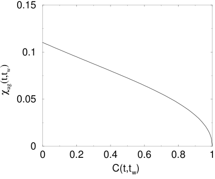
which shows that the ZFC susceptibility does not equilibrate, although the effect is not observable since $\chi_{st}(T_{F})$ diverges. As we shall see, in the $d=1$ Ising model it is not so, since the effect is observable. The best way to visualize the formation of $\chi^{*}$ is through the parametric plot. Since for $T_{F}=0$ the autocorrelation function is entirely given by $C_{ag}(t,t_{w})$, eliminating $x$ between Eqs. (198) and (211) one finds

$$\chi_{ag}(C)=\frac{1}{2\pi}\log\left\{\frac{2}{1+\frac{M_{0}^{2}}{C}\left[1-\sqrt{1-\frac{C^{2}}{M_{0}^{4}}}\right]}\right\}$$ (213)

whose plot is displayed in Fig.11 and is qualitatively similar to the one in Fig.12 for the $d=1$ Ising model. $\chi^{*}=0.1103$ is given by the intercept with the vertical axis at $C=0$.

5.2 Kinetic Ising model $d=1$

The one dimensional kinetic Ising model with the Glauber dynamics (131) is the other exactly soluble case [44] where, as in the large $N$ model, it is possible to derive analytically [39, 53, 54] the relaxation properties in the quench to $(d_{L},T_{F}=0)$, since for discrete symmetry $d_{L}=1$. As a matter of fact, one cannot straightforwardly set $T_{F}=0$, since, contrary to what happens for soft spins like in the GLW model, for hard spins the linear response function $R(t,t_{w})$ is not well defined for $T_{F}=0$. This is due to the dependence on the temperature and on the external field entering the dynamics through the transition rates (131) in the combination $h/T_{F}$, which does not allow for a linear response regime when $T_{F}\rightarrow 0$. There is not such a problem with the Langevin equation (133) where the temperature enters only through the noise, allowing to deal with a small external field also in the zero temperature limit. The problem can be bypassed by making the quench to a finite temperature $T_{F}$, where there are the linear regime and aging for $t_{w}\ll t_{eq}=\xi_{F}^{2}$, with

$$\xi_{F}=-[\ln\tanh(|J|/T_{F})]^{-1}.$$ (214)

Hence, aging lasts longer and longer as the temperature is lowered and $t_{eq}$ increases [39]. The behavior in the quench to $T_{F}=0$, then, must be understood as the limit for $T_{F}\rightarrow 0$ of the off-equilibrium behavior observed in the quenches to finite $T_{F}$. Alternatively, as can be seen immediately from Eq. (214), $t_{eq}$ diverges by letting the coupling constant $|J|\rightarrow\infty$ while keeping $T_{F}$ finite and, thus, preserving the linear regime.

With this proviso, let us derive $R(t,t_{w})$. From the exact solution of the model [39], the autocorrelation and autoresponse functions turn out to be related by

$$R(t,t_{w})={1\over 2T_{F}}\left[{\partial\over\partial t_{w}}C(t,t_{w})-{\partial\over\partial t}C(t,t_{w})\right].$$ (215)

Since for $T_{F}=0$, or equivalently for $|J|=\infty$, there are no thermal fluctuations and $G_{eq}(\tau,T_{F})$ vanishes, the autocorrelation function is entirely given by the aging component [55] and reads

$$C(t,t_{w})={2\over\pi}\arcsin\sqrt{\frac{2}{1+x}}.$$ (216)

The same is true also for $R(t,t_{w})$, since the stationary response $R_{eq}(\tau,T_{F})$ vanishes at $T_{F}=0$ and only the aging component gives a contribution. Inserting the above expression for $C(t,t_{w})$ into Eq. (215), $R(t,t_{w})$ is found to obey the scaling form (3)

$$R(t,t_{w})={1\over\sqrt{2}\pi T_{F}}t_{w}^{-1}(x-1)^{-1/2}$$ (217)

which implies $a=0$. Hence, as in the large $N$ model, it is an exact result that the exponent $a$ vanishes at $d_{L}$. The consequence, according to the general analysis of Section (4.3), is that the ZFC susceptibility does not equilibrate since the aging contribution does not disappear in the $t_{w}\rightarrow\infty$ limit. This feature is much more conspicuous here than in the large $N$ model, since now $\chi_{eq}(\tau,T_{F})$ vanishes identically and $\chi(t,t_{w})$ takes only the contribution of the aging component, obtained by integration of Eq. (217)

$$T_{F}\chi(t,t_{w})={1\over\sqrt{2}\pi}\left[{\pi\over 2}+\arcsin\left(1-{2\over x}\right)\right]$$ (218)

whose $x\rightarrow\infty$ limit gives

$$T_{F}\chi^{*}={1\over\sqrt{2}}.$$ (219)

The parametric representation, obtained eliminating $x$ with $C(t,t_{w})$ in Eq. (216)

$$T_{F}\widehat{\chi}(C)={\sqrt{2}\over\pi}\arctan\left[\sqrt{2}\cot\left({\pi\over 2}C\right)\right]$$ (220)

shows (Fig.12) an evident qualitative similarity with the behavior of $\chi_{ag}(C)$ in Fig.11. Finally, the FDR is obtained by differentiating $T_{F}\widehat{\chi}(C)$ with respect to $C$

$${\cal X}(C)=\left[2-\sin^{2}\left({\pi\over 2}C\right)\right]^{-1}$$ (221)

offering (Fig.13) an instance of the smooth and non universal behavior mentioned in section 4.6.

Figure 12: Plot of $T_{F}\chi$ against $C$ in the $d=1$ kinetic Ising model quenched to an arbitrary value of $T_{F}$ with $|J|=\infty$.

Figure 13: Parametric plot of the FDR in the $d=1$ kinetic Ising model quenched to an arbitrary value of $T_{F}$ with $|J|=\infty$.

6 The exponent $a$

As we have seen above, from the exact results of the large $N$ model and of the $d=1$ Ising model, the exponent $a$ vanishes in the quenches to $(d_{L},T_{F}=0)$. Although $a_{c}$, defined in Eq. (46), vanishes as $d\rightarrow d_{L}$ along the critical line, this is not an adequate explanation because, as pointed out in section 4.6, the quench to $(d_{L},T_{F}=0)$ is not a critical quench. Hence, the vanishing of $a$ must be accounted for within the framework of the response function in the quenches to below the critical line. Here, however, there is an additional complication due to a popular argument [56] identifying $a$, for $T_{F}<T_{C}$, with the exponent $n/z$ in the time dependence of the density of defects $\rho(t)\sim t^{-n/z}$, where $n=1$ or $n=2$ for scalar or vector order parameter [3]. In order to reproduce the argument, let us rewrite Eq. (66) specializing to the ZFC susceptibility

$$\langle\varphi(\vec{x},t)\rangle_{h}=\langle\varphi(\vec{x},t)\rangle+\int d\vec{y}\;\chi(\vec{x}-\vec{y},t,t_{w})h(\vec{y})+{\cal O}(h^{2})$$ (222)

and let us assume that $h(\vec{x})$ is an uncorrelated random field with expectations

$$\overline{h(\vec{x})}=0$$ (223)

and

$$\overline{h(\vec{x})h(\vec{y})}=h_{0}^{2}\delta(\vec{x}-\vec{y})$$ (224)

where the overbar denotes the average. Then, multiplying Eq. (222) by $h(\vec{x})$ and taking the average over the field one finds

$$\chi(t,t_{w})={1\over h_{0}^{2}}\overline{\langle\varphi(\vec{x},t)\rangle_{h}h(\vec{x})}$$ (225)

which shows that the ZFC susceptibility is proportional to the correlation of the local magnetization with the external random field on the same site. Writing the magnetization as the sum $\langle\varphi(\vec{x},t)\rangle_{h}=\langle\varphi(\vec{x},t)\rangle_{h,B}+\langle\varphi(\vec{x},t)\rangle_{h,D}$, where the first contribution comes from the bulk of domains, where equilibrium has been established, and the second from the defects, the above equation takes the form

$$\chi(t,t_{w})={1\over h_{0}^{2}}\left[\overline{\langle\varphi(\vec{x},t)\rangle_{h,B}h(\vec{x})}+\overline{\langle\varphi(\vec{x},t)\rangle_{h,D}h(\vec{x})}\right].$$ (226)

Associating the two terms in the right hand side to $\chi_{eq}$ and $\chi_{ag}$, respectively, and assuming that the defect contribution to the magnetization is proportional to the density of defects $\langle\varphi(\vec{x},t)\rangle_{h,D}\sim\rho(t)h(\vec{x})$ one finds

$$\chi_{ag}(t,t_{w})\sim\rho(t)$$ (227)

which eventually leads, recalling Eq. (98), to the identification

$$a_{\chi}=n/z.$$ (228)

Since for $T_{F}<T_{C}$ the dynamical exponent $z$ is independent of dimensionality, according to this argument also $a_{\chi}$ is independent of dimensionality, implying that there is no distinction between $a_{\chi}$ and $a$. Then, in the scalar case one ought to have $a=1/2$ and in the vector case $a=1$, independently from $d$ and, therefore, also at $d_{L}$.

This simple and intuitive picture is contradicted, as we have seen above, by the exact result for the large $N$ model, which gives $a_{\chi}$ dependent on $d$ for $d<d^{*}$, and by the vanishing of $a$, just found, in the $d=1$ Ising model. A point of contact with the prediction (228) is found only if one looks at $a_{\chi}$ in Eq. (208) for $d>d^{*}$. The question, then, is whether the large $N$ model and the $d=1$ Ising model are peculiar cases producing exceptions to the rule (228) or, viceversa, the lack of dimensionality dependence in (228) is indicative that in the intuitive argument some important element of the response mechanism is missed when $d<d^{*}$.

In order to attempt an answer one must enrich the phenomenology, necessarily resorting to approximate methods and to numerical simulations. Calculations of $a$ in the scalar GLW model, with the GAF approximation [33, 7] and an improved version of it [57], give

$$a=(d-1)/2$$ (229)

which shares with the large $N$ model the linear dependence on $d$ and reproduces the vanishing of $a$ at $d_{L}=1$, as in the Ising model. Furthermore, from the computation of the ZFC susceptibility [33, 7] one finds for $a_{\chi}$ the same pattern as in Eq. (208) for the large $N$ model

$$a_{\chi}=\left\{\begin{array}[]{ll}a=(d-1)/2,\qquad$for$\qquad d<d^{*}\\ 1/2,\qquad$with log corrections for$\qquad d=d^{*}\\ 1/2,\qquad$for$\qquad d>d^{*}\end{array}\right.$$ (230)

except that now $d^{*}=2$, in place of $d^{*}=4$ as in the large $N$ model. The details of the analytical computation show that the existence of the upper dimensionality $d^{*}$ occurs through the same mechanism as in the large $N$ model, namely with the microscopic time $t_{0}$ acting as a dangerous irrelevant variable at and above $d^{*}$.

Therefore, we may conclude that all the analytical results presented so far, exact and approximate, follow the same pattern which may be summarised by

$$a={n\over z}\left({d-d_{L}\over d^{*}-d_{L}}\right)$$ (231)

and

$$a_{\chi}=\left\{\begin{array}[]{ll}a,\qquad$for$\qquad d<d^{*}\\ n/z,\qquad$with log corrections for$\qquad d=d^{*}\\ n/z,\qquad$for$\qquad d>d^{*}\end{array}\right.$$ (232)

with $d^{*}$ greater than $d_{L}$ and dependent on the model.

Figure 14: $a\chi$ against $d$ in the kinetic Ising model. The dot for $d=1$ is the exact value. The dots for $d=2,3,4$ are the results of numerical simulations. The continous line is the plot of Eq. (232) with $n=1,z=2,d_{L}=1,d^{*}=3$. From Ref. [31].

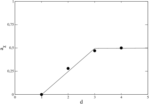
The next step is to see whether this pattern holds also for models accessible only through numerical simulations. The complication with simulations is that the measurement of the istantaneous response function $R(t,t_{w})$ is a very demanding task from the numerical point of view. Although significant progress has been made recently [13, 14, 15], yet a large scale survey of the behavior of $a$ upon varying $d$ in different models is unrealizable, as of now. The way out of the numerical bottleneck is to turn to the measurement of integrated response functions, such as the ZFC susceptibility, which are much less noisy than $R(t,t_{w})$ [31]. This program has been carried out through the measurement of $a_{\chi}$ on systems in different classes of universality [42], that is with scalar or vector order parameter, with and without conservation of the order parameter, and at different dimensionalities. The outcome fits into the pattern (232), provided one takes $d^{*}=3$ and $d^{*}=4$, respectively for scalar and vector order parameter and $z=3$ or $z=4$, for scalar conserved or vector conserved order parameter. As an example, the values of $a_{\chi}$ for the non conserved Ising model with dimensionality varying from $d=1$ to $d=4$ are plotted in Fig.14. Similar plots for other models can be found in Ref. [42]. For convenience the values of $d_{L},d^{*}$ and $a_{\chi}$ in the two analytically treatable cases and in the Ising model are collected in the following table

model	$d_{L}$	$d^{*}$	$a_{\chi}=a,d\leq d^{*}$	$a_{\chi},d>d^{*}$
large $N$	$2$	$4$	$(d-2)/2$	$1$
GAF scalar	$1$	$2$	$(d-1)/2$	$1/2$
Ising numerical	$1$	$3$	$(d-1)/4$	$1/2$

where the expression for $a_{\chi}$ in the last row of the Ising case must be understood as a phenomenological formula.

Despite the good amount of evidence supporting Eqs. (231) and (232), the issue of the exponent $a$ cannot be regarded as settled. The main reason is that a first principles derivation is lacking. Particularly challenging problems seem to be

1. what produces the deviation of $a_{\chi}$ from $n/z$ below $d^{*}$? Preliminary answers have been put forward [58, 42] on the basis of the roughening of interfaces for scalar models, but still much work remains to be done before a full understanding is reached.

2. in the scalar model treated with the GAF approximation, or its improved version [57], one finds $d^{*}=2$ while the fit of the numerical data requires $d^{*}=3$. This discrepancy reveals the strong non perturbative nature of the exponent $a$, for which even the best analytical tools presently available seem to be inadequate.

In conclusion, aging in domain growth is less trivial than commonly believed and poses some hard problems to our understanding of phase-ordering kinetics.

References

- [1] For reviews see: J.P.Bouchaud, L.F.Cugliandolo, J.Kurchan and M.Mezard, in Spin Glasses and Random Fields edited by A.P.Young (World Scientific, Singapore,1997). A.Crisanti and F.Ritort, J.Phys.A: Math.Gen. 36, R181 (2003). G.Biroli, A crash course on aging, cond-mat/0504681.
- [2] L.F.Cugliandolo, in Slow Relaxation and Non Equilibrium Dynamics in Condensed Matter , J.-L.Barrat, J.Dalibard, J.Kurchan and M.V.Feigel’man (Eds.) Les Houches - Ecole d’Ete de Physique Theorique, Vol. 77/2004 Springer-Verlag. Also available as cond-mat/0210312.
- [3] A.J.Bray, Adv.Phys. 43, 357 (1994).
- [4] G.F.Mazenko, O.T.Valls and M.Zannetti, Phys.Rev.B 38, 520 (1988).
- [5] L.C.E.Struick, Phyisical aging in amorphous polymers and other materials, Elsevier, Houston 1976.
- [6] S.Franz and M.A.Virasoro, J.Phys.A:Math.Gen. 33, 891 (2000).
- [7] E.Lippiello, F.Corberi and M.Zannetti, Eur.Phys.J.B 24, 359 (2001).
- [8] H.K.Janssen, B.Schaub and B.Schmittmann, Z.Phys.B:Cond.Math. 73, 539 (1989). H.K.Janssen, in “From Phase Transitions to Cahos - Topics in Modern Statistical Physiscs”, edited by G.Györgyi, I.Kondor, L.Saswári and T.Tel (World Scientific, Singapore, 1992).
- [9] P.Calabrese and A.Gambassi, J.Phys.A:Math.Gen. 38, R133 (2005).
- [10] T.Ohta, D.Jasnow and K.Kawasaki, Phys.Rev.Lett. 49, 1225 (1982).
- [11] Y.Oono and S.Puri, Mod.Phys.Lett. B 2, 861 (1988). G.F.Mazenko, Phys.Rev.Lett. 63, 1605 (1989); Phys.Rev.B 42, 4487 (1990); Phys.Rev.B 43, 5747 (1991). A.J.Bray and K.Humayun, Phys.Rev.E 48, R1609 (1993). S.De Siena and M.Zannetti, Phys.Rev.E 50, 2621 (1994).
- [12] F.Liu and G.F.Mazenko, Phys.Rev.B 44, 9185 (1991)
- [13] C.Chatelain, J.Phys.A:Math.Gen. 36, 10739 (2003). F.Ricci-Tersenghi, Phys.Rev.E 68, 065104(R) (2003).
- [14] E.Lippiello, F.Corberi, and M.Zannetti, Phys.Rev.E 71, 03610 (2005).
- [15] F.Corberi, E.Lippiello and M.Zannetti, Phys.Rev.E 72, 056103 (2005).
- [16] M.Henkel, M.Pleimling, C.Godrèche and J.M.Luck, Phys.Rev.Lett. 87, 265701 (2001). M.Henkel, Nucl.Phys. B 641, 405 (2002).
- [17] M.Pleimling and A.Gambassi, Phys.Rev.B 71, 180401 (2005).
- [18] E.Lippiello, F.Corberi, and M.Zannetti, Phys.Rev.E 74, 041113 (2006).
- [19] M.Henkel and M.Pleimling, J.Phys.:Condens.Matter 17, S1899 (2005); Ageing in disordered magnetys and local scale invariance, cond-mat/0607614.
- [20] M.Mezard, G.Parisi and M.Virasoro, Spin glass theory and beyond, World Scientific, Singapore 1987.
- [21] R.G.Palmer, Adv.Phys. 31, 669 (1982).
- [22] C.Godrèche and J.M.Luck, J.Phys.:Condens.Matter 14, 1589 (2002).
- [23] P.C.Hohenberg and B.I.Halperin, Rev.Mod.Phys. 49, 435 (1977).
- [24] D.A.Huse, Phys.Rev.B 40, 304 (1989).
- [25] see for example in D.P.Landau and K.Binder, A guide to Monte Carlo simulations in statistical physics, Cambridge University Press, 2000.
- [26] F.C.Wang and C.K.Hu, Phys.Rev.E 56, 2310 (1997).
- [27] H.Furukawa, J.Stat.Soc.Jpn. 58, 216 (1989); Phys.Rev.B 40, 2341 (1989).
- [28] D.S.Fisher and D.A.Huse, Phys.Rev.B 38, 304 (1989).
- [29] J.P.Bouchaud, J.Phys.I (France) 2, 1705 (1992).
- [30] L.F.Cugliandolo and J.Kurchan, Phys.Rev.Lett. 71, 173 (1993); J.Phys.A:Math.Gen. 27, 5749 (1994).
- [31] F.Corberi, E.Lippiello and M.Zannetti, Phys.Rev.E 68, 046131 (2003).
- [32] M.Fisher, Scaling, universality and renormalization group theory Appendix D, Lectures Notes in Physics 186, Springer-Verlag.
- [33] L.Berthier, J.L.Barrat and J.Kurchan, Eur.Phys.J.B 11, 635 (1999).
- [34] F.Corberi, E.Lippiello and M.Zannetti, Phys.Rev.E 65, 046136 (2002).
- [35] K.H.Fischer and J.A.Hertz, Spin Glasses, Cambridge University Press, 1991. H.Yoshino, K.Hukushima and H.Takayama, Phys.Rev.B 66, 064431 (2002).
- [36] G.Parisi, F.Ricci-Tersenghi and J.J.Ruiz-Lorenzo, Eur.Phys.J. B 11, 317 (1999).
- [37] L.F.Cugliandolo, J.Kurchan and L.Peliti, Phys.Rev.E 55, 3898 (1997).
- [38] C.Godrèche and J.M.Luck, J.Phys.A:Math.Gen. 33, 9141 (2000).
- [39] E.Lippiello and M.Zannetti, Phys.Rev.E 61, 3369 (2000).
- [40] C.Godrèche and J.M.Luck, J.Phys.A:Math.Gen. 33, 1151 (2000).
- [41] F.Corberi, C.Castellano, E.Lippiello and M.Zannetti, Phys.Rev.E 65, 066114 (2002).
- [42] F.Corberi, C.Castellano, E.Lippiello and M.Zannetti, Phys.Rev.E 70, 017103 (2004).
- [43] E.Lippiello, F.Corberi and M.Zannetti, Phys.Rev.E 71, 036104 (2005).
- [44] R.J.Glauber, J.Math.Phys. 4, 294 (1963).
- [45] N.Goldenfeld, Lectures on phase transitions and the renormalization group, Addison-Wesley, 1992.
- [46] P.M.Chaikin and T.C.Lubensky, Principles of condensed matter physics, Cambridge University Press, 1995. S.K.Ma, Modern theory of critical phenomena, W.A.Benjamin, Inc., 1976.
- [47] L.F.Cugliandolo and D.S.Dean, J.Phys.A 28, 4213 (1995).
- [48] C.Chamon, L.F.Cugliandolo and H.Yoshino, JSTAT: Theory and Experiment, P01006 (2006).
- [49] R.J.Baxter, Exactly Solved Models in Statistical Mechanics (Academic Press, New York, 1982).
- [50] C.Castellano, F.Corberi and M.Zannetti, Phys.Rev.E 56, 4973 (1997).
- [51] T.J.Newman and A.J.Bray, J.Phys.A:Math.Gen. 23, 4491 (1990).
- [52] G.F.Mazenko and M.Zannetti, Phys.Rev.Lett. 53, 2106 (1984); Phys.Rev.B 32, 4565 (1985).
- [53] C.Godrèche and J.M.Luck, J.Phys.A:Math.Gen. 33, 1151 (2000).
- [54] P.Mayer and P.Sollich, J.Phys.A:Math.Gen. 37 9 (2004).
- [55] A.J.Bray, J.Phys.A:Math.Gen. 22, L67 (1989). A.Prados, J.J.Brey and B.Sánchez-Rey, Europhys.Lett. 40, 13 (1997).
- [56] A.Barrat, Phys.Rev.E 57, 3629 (1998).
- [57] G.F.Mazenko, Phys.Rev.E 69, 016114 (2004).
- [58] M.Henkel, M.Paessens and M.Pleimling, Phys.Rev.E 69, 056109 (2004).