Testing statics-dynamics equivalence at the spin-glass transition in three dimensions

Abstract

The statics-dynamics correspondence in spin glasses relate non-equilibrium results on large samples (the experimental realm) with equilibrium quantities computed on small systems (the typical arena for theoretical computations). Here we employ statics-dynamics equivalence to study the Ising spin-glass critical behavior in three dimensions. By means of Monte Carlo simulation, we follow the growth of the coherence length (the size of the glassy domains), on lattices too large to be thermalized. Thanks to the large coherence lengths we reach, we are able to obtain accurate results in excellent agreement with the best available equilibrium computations. To do so, we need to clarify the several physical meanings of the dynamic exponent close to the critical temperature.

The glass transition, the dramatic dynamic slowdown experienced by spin-glasses, fragile molecular glasses, polymers, colloids, etc., upon approaching their glass temperature $T_{\mathrm{g}}$, has long puzzled scientists Cavagna (2009) The phenomenon has been long suspected to be caused by the growth of a characteristic length Adam and Gibbs (1965), an issue under current investigation Weeks et al. (2000); Berthier et al. (2005); Gutiérrez et al. (2014).

Spin-glasses enjoy a privileged status in this context, for a number of reasons. First, their glass transition is a bona fide phase transition at $T_{\mathrm{c}}=T_{\mathrm{g}}$ Gunnarsson et al. (1991); Palassini and Caracciolo (1999); Ballesteros et al. (2000). Second, consider a rapid quench from high-temperature to the working temperature $T<T_{\mathrm{c}}$, where the system is left to equilibrate for a time $t_{\mathrm{w}}$. The system remains perennially out equilibrium. This aging process Vincent et al. (1997) consists in the growth of glassy magnetic domains (which reminds coarsening Bray (1994)). The size of these domains $\xi(t_{\mathrm{w}})$ is experimentally accesible, and it can be as large as 100 lattice spacings Joh et al. (1999); Bert et al. (2004) (enormously larger than any length scale identified on molecular liquids Berthier et al. (2005); Gutiérrez et al. (2014)).Third, the growth of $\xi(t_{\mathrm{w}})$ has been well studied numerically Rieger (1993); Kisker et al. (1996); Marinari et al. (2000a, b); Berthier and Bouchaud (2002); Berthier and Young (2005); Jaubert et al. (2007); Belletti et al. (2008a, 2009); Manssen and Hartmann (2014). In particular, the dedicated Janus computer Belletti et al. (2008b) has allowed to cover $t_{\mathrm{w}}$ ranging from picoseconds to 0.1 seconds Belletti et al. (2008a, 2009).Fourth, a statics-dynamics correspondence is expected Franz et al. (1998): detailed dictionaries have been built Barrat and Berthier (2001); Alvarez Baños et al. (2010), relating equilibrium results on finite systems (the typical setting for numerical simulations) with non-equilibrium results on macroscopic (or mesoscopic) samples.

The statics-dynamics equivalence is particularly exciting, because it brings the much awaited possibility of detailed comparisons between experimental results and theoretical computations. In fact, experimental effort has been recently devoted to the measurement of $\xi(t_{\mathrm{w}})$ with that end Joh et al. (1999); Jönsson et al. (2002); Bert et al. (2004); Nakamae et al. (2012); Guchhait and Orbach (2014). Unfortunately, appealing as it is, the static-dynamic equivalence has not yet produced new insights (in fact, not even the mutual consistency of different dictionaries Barrat and Berthier (2001); Alvarez Baños et al. (2010) has been shown).

Here, we obtain a complete characterization of the critical behavior of the three-dimensional Ising spin-glass based solely on the statics-dynamics equivalence. Our Monte Carlo simulations follow the growth of $\xi(t_{\mathrm{w}})$ on lattices too large to be equilibrated. In this way, we obtain the largest coherence lengths ever obtained in a simulation (up to 25 lattice spacing). Thus armed, we obtain fairly accurate estimates of the critical exponents. Our results are completely consistent with the best equilibrium computations on small lattices Hasenbusch et al. (2008a); Baity-Jesi et al. (2013). Our analysis is obviously related to dynamic scaling Ozeki and Ito (2007), with an important difference. We find it mandatory to eliminate time, in favour of the coherence length $\xi(t_{\mathrm{w}})$. The reason, explained below, is in that the dynamic exponent $z$ changes its physical meaning at $T_{\mathrm{c}}$. Last, but not least, we show in Appendix A how to perform on conventional processors investigations previously regarded as impossible without special computers.

The Hamiltonian for the $D\!=\!3$ Edwards-Anderson model with nearest-neighbors interactions is

$${\cal H}=-\sum_{\langle\boldsymbol{x},\boldsymbol{y}\rangle}J_{\boldsymbol{x},\boldsymbol{y}}\,\sigma_{\boldsymbol{x}}\,\sigma_{\boldsymbol{y}}\,.$$ (1)

The spins $\sigma_{\boldsymbol{x}}=\pm 1$ are placed on the nodes, $\boldsymbol{x}$, of a cubic lattice of linear size $L=256$ and periodic boundary conditions. The couplings $J_{\boldsymbol{x},\boldsymbol{y}}=\pm 1$ are chosen randomly with $50\%$ probability, and are quenched variables. Each coupling choice is named a sample. We denote by $\overline{(\cdot\cdot\cdot)}$ the average over the couplings. Model (1) undergoes a spin-glass transition at $T_{\mathrm{c}}=1.1019(29)$ Baity-Jesi et al. (2013).

We study the direct quench, the simplest dynamic protocol. At the starting time $t_{\mathrm{w}}=0$, the system is in a random configuration (i.e. $T=\infty$). We place it instantaneously at the working temperature $T$ and follow the evolution as $t_{\mathrm{w}}$ increases, Fig. 1. Our time unit is the Monte Carlo step (a full lattice Metropolis sweep).

Metropolis dynamics belongs to the Universality Class of the physical evolution (it is an instance of the so-called model A dynamics Hohenberg and Halperin (1977)), and is straightforward to implement Landau and Binder (2005). However, our aim is to reach large $L$ and $t_{\mathrm{w}}$. Rather than resorting to special hardware Belletti et al. (2008b); Manssen and Hartmann (2014); Lulli et al. (2014a); Fang et al. (2014); Feng et al. (2014), we employ synchronous multi-spin coding on standard CPUs. In a naive implementation random number generation is a major cost. However, our minimal energy barrier is 4, rarely overcome at the temperatures of interest [for instance, exp(-4/$T_{\mathrm{c}}$)$\approx$ 0.026]. Hence, the Gillespie method Gillespie (1977); Bortz et al. (1975) allows for major savings (see Appendix A).

We compute the coherence-length from the correlation function of the replica field $q_{\boldsymbol{x}}(t_{\mathrm{w}})\equiv\sigma_{\boldsymbol{x}}^{(a)}(t_{\mathrm{w}})\sigma_{\boldsymbol{x}}^{(b)}(t_{\mathrm{w}})\,$:

$$C_{4}(\boldsymbol{r},t_{\mathrm{w}})=\overline{L^{-3}\sum_{\boldsymbol{x}}q_{\boldsymbol{x}}(t_{\mathrm{w}})q_{\boldsymbol{x}+\boldsymbol{r}}(t_{\mathrm{w}})}\,.$$ (2)

We restrict the displacement $\boldsymbol{r}$ to a lattice axis and compute integrals $I_{k}(t_{\mathrm{w}})=\int_{0}^{\infty}\mathrm{d}\,r\,r^{k}C_{4}(r,t_{\mathrm{w}})\,$. Then, $\xi_{1,2}(t_{\mathrm{w}})=I_{2}(t_{\mathrm{w}})/I_{1}(t_{\mathrm{w}})$ Belletti et al. (2008a, 2009). In all cases, we find $L>10\,\xi_{1,2}(t_{\mathrm{w}})$ hence we regard our data as representative of the thermodynamic limit Belletti et al. (2008a).

Fig. 1 shows a rather accurate algebraic growth, $\xi(t_{\mathrm{w}})\sim t_{\mathrm{w}}^{1/z(T)}$ Joh et al. (1999); Marinari et al. (2000a). Yet, there is some controversy. On the one hand, low-temperature data suggest $z(T\leq T_{\mathrm{c}})\approx z_{\mathrm{c}}T_{\mathrm{c}}/T$ Joh et al. (1999); Marinari et al. (2000a); Belletti et al. (2008a, 2009). On the other hand, in Ref. Liu et al. (2014) a temperature varying protocol with $T\geq T_{\mathrm{c}}$ produced a numerical value [$z_{\mathrm{c}}=5.85(9)$ for $J=\pm 1$ or $z_{\mathrm{c}}=6.00(19)$ for Gaussian couplings] hardly consistent with the low-temperature $z_{\mathrm{c}}=6.86(16)$ Belletti et al. (2008a, 2009).

Our own data, Fig. 1–right, suggest an exponent $z(T)$ discontinuous at $T_{\mathrm{c}}$. Of course, this might be an effect of our $z(T)$ being an effective exponent (due to our fitting time-window). But this is not a logical necessity.

Indeed, exponent $z(T)$ carries different meanings. For $T<T_{\mathrm{c}}$ it describes (glassy) coarsening: the coherence length grows forever as $\xi(t_{\mathrm{w}})\sim t_{\mathrm{w}}^{1/z(T)}$. Yet, $z(T>T_{\mathrm{c}})$ is concerned with equilibration. One has a characteristic time $\tau(T)$ (when $\xi(\tau,T)$ reaches, say, $90\%$ of the equilibrium $\xi_{\mathrm{eq}}$) and then $\tau(T)\propto[\xi_{\mathrm{eq}}(T)]^{z^{*}}$. In fact, for the simplest non-trivial model (the $D=2$ Ising ferromagnet) the coarsening exponent is $z_{\mathrm{FM}}(T<T_{\mathrm{c}}^{{\mathrm{FM}}})=2$ Bray (1994), while $z^{*}_{\mathrm{c},\mathrm{FM}}=2.1667(5)$ Nightingale and Blöte (2000) for critical equilibration.

Clearly, this delicate cross-over will require further investigation. Yet, we have rationalized why a $T\geq T_{\mathrm{c}}$ protocol Liu et al. (2014) produces $z(T>T_{\mathrm{c}})\approx 6$.

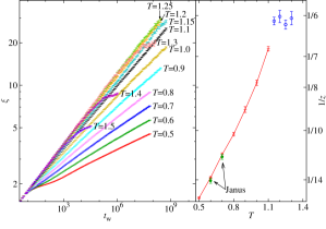
Figure 1: (Color online) Left: Coherence length $\xi_{12}(t_{\mathrm{w}})$ vs. Monte Carlo time, as computed for model (1) on lattices of size $L=256$, for several temperatures [$T_{\mathrm{c}}=1.1019(29)$ Baity-Jesi et al. (2013)]. One Monte Carlo step corresponds to 1 picosecond in physical time Mydosh (1993). For $T\geq 1.3$, we reach equilibrium. Right: Dynamic exponent $z(T)$ computed in the non-equilibrium regime $\xi(t_{\mathrm{w}})\sim t_{\mathrm{w}}^{1/z(T)}$. Joined red points stand for $T\leq T_{\mathrm{c}}$. Note the constant value $z(T>T_{\mathrm{c}})\approx 6$ (blue circles). We perform the fits for $t_{\mathrm{w}}>2^{20}\approx 10^{6}$ Monte Carlo steps (but for $T=1.3$ where $2^{16}\leq t_{\mathrm{w}}\leq 2^{20}$, in order to avoid thermalization). We also show Janus data Belletti et al. (2009) (green circles), computed for longer times. We only show the $L=80$ Janus data at temperatures free from finite-size artifacts.

These complications reinforce our choice of basing finite-time scaling on $\xi_{1,2}(t_{\mathrm{w}})$, rather than on $t_{\mathrm{w}}$ Nakamura et al. (2003); Ozeki and Ito (2007); Romá (2010). To do so, we adapt Binder’s method Binder (1981) (in Appendix C we explore another possibility Nakamura (2010) that turns out to be less accurate). Let $q(B_{l},t_{\mathrm{w}})=\sum_{{}_{\boldsymbol{x}}\in B_{l}}q_{\boldsymbol{x}}(t_{\mathrm{w}})/l^{3}$ be the average of the replica field on a cubic box of side $l$. We compute $q_{k}(l,t_{\mathrm{w}})=\overline{q^{k}(B_{l},t_{\mathrm{w}})}$, its $k$-th power averaged over samples, replica parings, as well as over boxes $B_{l}$. Binder’s ratio $U_{4}(l,t_{\mathrm{w}},T)=\overline{q_{4}(l,t_{\mathrm{w}})}/\overline{q_{2}(l,t_{\mathrm{w}})}^{2}$ is a dimensionless parameter likely to display Universal behavior (for instance, $U_{4}(l,t_{\mathrm{w}},T)\to 3$ when $l\gg\xi(t_{\mathrm{w}})$ due to the Central Limit Theorem, see also Ref. Marinari et al. (1996)).

The analogy with Finite Size Scaling impels us to change variables: $y=[T-T_{\mathrm{c}}][\xi(t_{\mathrm{w}},T)]^{1/\nu}$ and $\lambda=l/\xi(t_{\mathrm{w}},T)$. Then, barring subleading corrections to scaling, we expect:

$$U_{4}(l,t_{\mathrm{w}},T)=f(y,\lambda)+[\xi(t_{\mathrm{w}})]^{-\omega}g(y,\lambda),$$ (3)

where $\nu$ is the correlation-length critical exponent, $\omega$ is the leading corrections to scaling exponent, and $f$ and $g$ are dimensionless scaling functions. Note that the independent variables in the l.h.s. of Eq. (3) ($l$, $t_{\mathrm{w}}$ and $T$) are discrete. Yet, the r.h.s. variables ($\xi,y$ and $\lambda$) are continuous. We solve this problem by means of polynomial interpolations (see Appendix B). Errors are estimated with the jackknife method Amit and Martin-Mayor (2005), computed over the samples.

Fig. 2 contains a qualitative discussion of Eq. (3). In the inset, we show data at $y=0$ (i.e. $T=1.1$, an excellent approximation to $T_{\mathrm{c}}$ Baity-Jesi et al. (2013)). For large $\xi(t_{\mathrm{w}})$, $U_{4}$ converges to the scaling function $f(0,\lambda)$. On the other hand, in Fig. 2–main we show that Eq. (3) actually describes a cross-over in temperature. Let us fix $\lambda=1$ and $T>T_{\mathrm{c}}$. Then, $y$ becomes large and positive as $\xi(t_{\mathrm{w}},T)$ grows. We see that $U_{4}$ approach a high-temperature limit (a $\lambda$-dependent renormalized coupling constant Parisi (1988)). At $T_{\mathrm{c}}$ we have the critical limit because $y=0$ no matter how large $\xi(t_{\mathrm{w}})$ is. In the spin-glass phase, $y$ becomes large and negative. For large $\xi$ we reach a low-temperature limit, that has been much debated in the past Marinari et al. (1998); Newman and Stein (1998).

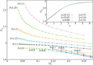
Figure 2: (Color online) Binder’s ratio as a function of $[\xi(t_{\mathrm{w}},T)]^{-1}$, computed for fixed dimensionless box-size $\lambda=1$ and several temperatures [recall that $\lambda=l/\xi(t_{\mathrm{w}})$]. Inset: Critical Binder’s ratio as a function of the dimensionless box-size for several $\xi(t_{\mathrm{w}})$ ($T=1.1\approx T_{\mathrm{c}}$). As expected by plugging $y=0$ in Eq. (3), the curve is scale-invariant when the small $\xi$ corrections fade away.

In order to compute the critical exponents, we decided to follow the fixed-height method Hasenbusch et al. (2008b); Baños et al. (2012a). For a fixed height $h$, and fixed $\lambda$ and $\xi(t_{\mathrm{w}},T)$, we seek the temperature $T_{h,\lambda,\xi}$ such that $U_{4}=h$. Eq. 3 tells us that

$$T_{h,\lambda,\xi}=T_{\mathrm{c}}+A_{h,\lambda}\xi^{-1/\nu}+B_{h,\lambda}\xi^{-(\omega+1/\nu)}\ldots\,,$$ (4)

where $A_{h,\lambda}$ and $B_{h,\lambda}$ are scaling amplitudes and the dots stand for higher-order corrections to scaling. We compute $T_{\mathrm{c}}$, $\nu$ and $\omega$ by performing joint fits to data for severals $\lambda$ and $h$, see Fig. 3 (unfortunately, the fit lacks any predictive power for exponent $\omega$, hence we shall borrow $\omega=1.12(10)$ from Baity-Jesi et al. (2013)). In order to perform these fits, we considered a fixed grid of coherence lengths $\xi_{n}=2^{n/8}$.

A major problem when fitting to Eq. (4) is that of the singular covariance matrix (we have many data points, but only 50 independent samples). We solve it following Belletti et al. (2008a, 2009): we fit taking into account only the diagonal part of the covariance matrix. We perform a fit for each jackknife block, and compute the final errors from the fluctuations of these fits. We compute as well the diagonal goodness-of-fit indicator $\chi^{2}_{\mathrm{diagonal}}$ (the sum of the squared deviations of data from fit, in units of their statistical error). This fitting procedure was tested in Ref. Belletti et al. (2009) and found to be reasonably stable for $\chi^{2}_{\mathrm{diagonal}}$ as small as half the number of degrees of freedom.

We included in our fit results for $\lambda=0.75,1,1.25$ and $1.5$. A crucial issue is selecting $\xi_{\mathrm{min}}$, the minimal $\xi$ considered in the fit. A tradeoff should be found. The larger is $\xi_{\mathrm{min}}$, the smaller are the systematic errors, but the larger becomes the statistical uncertainty. We find a stable fit for $\xi_{\mathrm{min}}\geq 2^{9/4}\approx 4.75$ ($\chi^{2}_{\mathrm{diagonal}}/\text{d.o.f.}=583/665$ if $\xi_{\mathrm{min}}=2^{9/4}$). However, as we enlarge $\xi_{\mathrm{min}}$ we find that $\chi^{2}_{\mathrm{diagonal}}/\text{d.o.f}$ decreases monotonically while the statistical error increases. We decided to stop at the $\xi_{\mathrm{min}}$ such that $\chi^{2}_{\mathrm{diagonal}}/\text{d.o.f.}\approx 0.5$ because errors start increasing wildly at that point. This corresponds to $\xi_{\mathrm{min}}=2^{23/8}\approx 7.33$ ($\chi^{2}_{\mathrm{diagonal}}/\text{d.o.f.}=229/482$). The final result for our fit to Eq. (4) is

$$T_{\mathrm{c}}=1.115(15)\,,\ \nu=2.2(3)\,.$$ (5)

For comparison, recall the equilibrium results $T_{\mathrm{c}}=1.1019(29)$, $\nu=2.56(4)$ and $\omega=1.12(10)$ Baity-Jesi et al. (2013). Varying $\omega$ within the bounds of Baity-Jesi et al. (2013) produces negligible changes in the results in Eq. (5). It is also interesting to see what happens fixing $\nu$ and $\omega$ in the fit to the central values of Baity-Jesi et al. (2013) ($\xi_{\mathrm{min}}\geq 2^{23/8}$, $\chi^{2}_{\mathrm{diagonal}}/\text{d.o.f.}=241/483$):

$$T_{\mathrm{c}}=1.102(8)\,,$$ (6)

in excellent agreement with the equilibrium result.

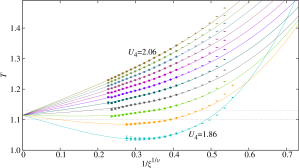
Figure 3: (Color online) Joint fit to Eq. (4) for $\lambda=0.75$. The $U_{4}$ spacing is 0.02. For all fits, the values of $T_{\mathrm{c}}$, $\nu$ and $\omega$ are held common. Big data points were included in the fit. The horizontal dotted lines correspond to $T_{\mathrm{c}}\pm\Delta T_{\mathrm{c}}$ from Eq. (5).

The anomalous dimension $\eta$ can be computed by working directly at $T=1.1\approx T_{\mathrm{c}}$. We select two times $t_{\mathrm{w}}^{(1)}$ and $t_{\mathrm{w}}^{(2)}$ such that $\xi(t_{\mathrm{w}}^{(1)},T_{\mathrm{c}})=\xi$ and $\xi(t_{\mathrm{w}}^{(2)},T_{\mathrm{c}})=2\xi$. Then the ratio of integrals is

$$I_{2}(t_{\mathrm{w}}^{(2)},T_{\mathrm{c}})/I_{2}(t_{\mathrm{w}}^{(1)},T_{\mathrm{c}})=2^{2-\eta}+C_{I}/\xi^{\omega}+\ldots$$ (7)

The problem with Eq. (7) is that the amplitude for scaling corrections $C_{I}$ seems vanishing (within errors), so one could be afraid that we overestimate the error. Anyhow, for $\xi_{\text{min}}=2^{7/4}\approx 3.36$ we obtain $\eta=-0.380(7)$ and $\chi^{2}_{\mathrm{diagonal}}/\text{d.o.f.}=10.4/14$, to be compared with $\eta=-0.3900(36)$ Baity-Jesi et al. (2013) (for larger $\xi_{\text{min}}$ fits are stable but $\chi^{2}_{\mathrm{diagonal}}/\text{d.o.f.}$ drops well below 0.5). Changing $\omega$ within the bounds of Baity-Jesi et al. (2013) produces a negligible change. We estimate that the error induced in $\eta$ by the uncertainty in $T_{\mathrm{c}}$ Baity-Jesi et al. (2013) is comparable with the statistical error obtained at $T=1.1$.

Incidentally, one may use the ratio of integrals $I_{2}(t_{\mathrm{w}}^{(2)},T)/I_{2}(t_{\mathrm{w}}^{(1)},T)$ as a (very noisy) substitute of the Binder’s cumulant in Eqs. (3,4) (see Appendix C). In fact, one may view the temperature crossover in Eq. (3) as a crossover for the $C_{4}(r,t_{\mathrm{w}})$ correlation function (2). Indeed, for all the $T$ and $t_{\mathrm{w}}$ in this work, the functional form Marinari et al. (1996)

$$C_{4}(r,t_{\mathrm{w}})\sim\text{e}^{-[r/\xi(t_{\mathrm{w}})]^{b}}/r^{\theta}\,,$$ (8)

fits satisfactorily our data. For small $y$ [i.e. at $T_{\mathrm{c}}$ or for small $\xi(t_{\mathrm{w}})$] data follows Eq. (8) with critical parameters. However, as the coherence-length grows, these parameters are not adequate neither for the paramagnetic phase (at or near equilibrium, see Fig. 4), nor for the spin-glass phase Belletti et al. (2008a, 2009).

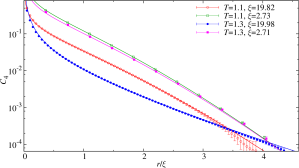
Figure 4: (Color online) Temperature-dependent dynamic crossover in the spatial correlation function $C_{4}(r,t_{\mathrm{w}})$ (2). We show $C_{4}$ vs. the dimensionless $r/\xi(t_{\mathrm{w}})$, both at $T_{\mathrm{c}}$ and deep in the paramagnetic phase ($T=1.3$). For small coherence length, $\xi(t_{\mathrm{w}})\approx 2.7$, data for both temperatures can be fit to Eq. (8) with critical parameters $b\approx 1.46$ (this work) and $\theta\approx D-2+\eta=0.610(4)$ Baity-Jesi et al. (2013), see the continuous lines in the plot. The same parameters work for data at $T_{\mathrm{c}}$ and $\xi(t_{\mathrm{w}})\approx 20$. However, for such a large coherence-length, data at $T=1.3$ are better fitted with the three-dimensional free-field (Gaussian) parameters $(b=1,\theta=1)$.

In this work, we have employed (for the first time, we believe) statics-dynamics equivalence Alvarez Baños et al. (2010) to obtain some new physical results. In particular, we have shown how one can study the spin-glass transition in the dynamic regime relevant to most experiments: non-equilibrium data on systems much larger than the coherence length. Once we trade waiting time by coherence length, standard finite-size scaling methods Binder (1981) are very successful at describing the temperature-dependent dynamic crossover (a real phase transition with temperature takes place only for infinite coherence length). It is then possible that the finite-size crossover found in equilibrium Baity-Jesi et al. (2014) is the driving force behind the apparent Universality violations found experimentally Bouchiat (1986); Lévy (1988); Petit et al. (2002); Bert et al. (2004); Campbell and Petit (2010). However, an alternative explanation, logically possible but rather dramatic, is that Universality does not hold in spin glasses Mari and Campbell (1999); Pleimling and Campbell (2005).

Regarded as a numerical method to compute critical exponents, we note that our thermodynamic limit approach is less accurate than finite-size methods Hasenbusch et al. (2008b); Baity-Jesi et al. (2013); Lulli et al. (2014b) which is hardly a surprise.

We conclude by mentioning the two major difficulties (in our opinion) for an analogous experimental study. On the one hand, one needs to reach spatial resolution to study the correlation function $C_{4}(r,t_{\mathrm{w}})$. Progress in this direction are still incipient. Spatial resolution has been reached only for a structural glass Oukris and Israeloff (2010). For spin-glasses, recent experimental efforts focus on confining geometries Komatsu et al. (2011); Guchhait and Orbach (2014) (which can be seen as an indirect way to study the correlation function). On the other hand, the direct quench is a rather crude approximation: the experimental sample never reaches the working temperature instantaneously Rodriguez et al. (2003, 2013). The protocol of Ref. Liu et al. (2014) is, probably, more suitable to model the experimental setup. However, as Fig. 1 shows, mixing temperatures in the dynamic evolution is a delicate procedure that requires further investigation.

We thank Enzo Marinari, Giorgio Parisi and Andrea Maiorano for helping us with our first Pthreads programs. We also thank Andrea Pelissetto, Giorgio Parisi and Matteo Lulli for discussing with us, prior to publication, their very interesting and accurate finite-time, finite-size scaling approach Lulli et al. (2014b). We thank as well Juan Jesús Ruiz-Lorenzo, Peter Young and David Yllanes for discussions.

The total simulation time devoted to this project was the equivalent of 36 days of the full (3072 AMD cores) Memento cluster (see http://bifi.es). We were partly supported by MINECO (Spain) through research contract N^o FIS2012-35719-C02.

Appendix A Synchronous Multispin coding

Modern CPUs, both Intel and AMD, support 256-bit words in their streaming extensions. This means that one can perform basic Boolean operations (AND, XOR, etc.) in parallel for all the 256 bits. Now, it is well known that the Metropolis update of a single spin can be cast into a sequence of boolean operations, see e.g. Newman and Barkema (1999). One can use this idea to simulate several, up to 256, independent systems. This approach, named asynchronous multispin coding, has been used many times, see Refs. Leuzzi et al. (2008); Baños et al. (2012b); Fernandez et al. (2010); Baity-Jesi et al. (2013); Manssen and Hartmann (2014); Lulli et al. (2014a) for instance. Ref. Fang et al. (2014); Feng et al. (2014) offers a creative alternative: In their Parallel Tempering simulation each bit represent an independent system copy (all of them evolve under the same couplings, but at different temperatures Hukushima and Nemoto (1996); Marinari (1998)). Instead, our aim is to exploit the streaming extensions to speed-up the simulation of a single system (which is named synchronous multispin coding).

The main problem with synchronous multispin coding is that we need 256 independent random numbers, if the 256 spins coded in a word belong to the same physical system. This breaking of parallelism is usually regarded as a major inconvenience (see, however, Ref. Liu et al. (2014)).

For the sake of clarity, we shall first explain our geometrical set up and then describe how one can use the Gillespie method Gillespie (1977); Bortz et al. (1975) to reduce drastically the number of needed random numbers.

A.1 Our multispin coding geometry

Physical spins sit on the nodes of a $L=256$ lattice with periodic boundary conditions. Euclidean coordinates then run as $0\leq x,y,z\leq 255$. Each physical spin is a binary variable to be coded in a single bit, $s_{(x,y,z)}=\pm 1$.

We pack 256 physical spins into one superspin. Our superspins sit in the nodes of a different lattice. It will be also a cubic lattice with periodic boundary conditions (the overall geometry is that of a parallelepiped, rather than a cube). The major requirement is that nearest-neighbor spins in the physical lattice should be as well nearest neighbors in the superspin lattice. Our solution is as follows.

Superspins are placed at the nodes of a cubic lattice with dimensions $L_{x}=L_{y}=L/8$, and $L_{z}=L/4$. The relation between physical coordinates $(x,y,z)$ and the coordinates in the superspin lattice $(i_{x},i_{y},i_{z})$ is

$$x = b_{x}L_{x}+i_{x}\,,\ 0\leq i_{x}<L_{x}\,,\ 0\leq b_{x}<8\,,$$

$$y = b_{y}L_{y}+i_{y}\,,\ 0\leq i_{y}<L_{y}\,,\ 0\leq b_{y}<8\,,$$ (9)

$$z = b_{z}L_{z}+i_{z}\,,\ 0\leq i_{z}<L_{z}\,,\ 0\leq b_{z}<4\,.$$

In this way, exactly 256 sites in the physical lattice are given the same superspin coordinates $(i_{x},i_{y},i_{z})$. We differenciate between them by means of the bit index:

$$i_{b}=64b_{z}+8b_{y}+b_{x}\,,\ 0\leq i_{b}\leq 255\,.$$ (10)

An added bonus of Eq. (9) is that the parity of the original site, namely the parity of $x+y+z$, coincides with the parity of the corresponding superspin site $i_{x}+i_{y}+i_{z}$. In fact, the single cubic lattice is bipartite. It can be regarded as two interleaved face-centered cubic lattice. A given site is said to belong to the even or the odd sublattice according to the parity of $x+y+z$. For models with only nearest-neighbors interactions, sites belonging to (say) the even sublattice interact only with the odd sites.

An important consequence of the even-odd decomposition is that it eases parallelism. Indeed, we define the full lattice Metropolis sweep as the update of all the $L^{3}/2$ even sites, followed by the update of all the $L^{3}/2$ odd sites. The bipartite nature of the lattice makes it irrelevant the updating order of sites of a given parity. Hence, several updating threads may legitimately concur on the same lattice, provided that all of them simultaneously access only sites of the same parity.

A.2 Saving random numbers

For our synchronous multispin coding we do need to generate 256 random numbers in order to update a single superspin. Yet, it has been realized several times that most of the effort in generating (pseudo) random numbers is wasted when simulating discrete models at low temperatures Gillespie (1977); Bortz et al. (1975). In fact, at a given time the simulation may try to overcome an energy barrier $\Delta E$. However, we should overcome it only with probability $\text{e}^{-\Delta E/T}$. In other words, we waste $\sim\text{e}^{\Delta E/T}$ random numbers (that deny us the permit to overcome the barrier) until we generate one random number that really allows us to walk uphill in energy. Let us plug some numbers for our model, where the possible barrier heights are $\Delta E=4,8$ or $12$. So, at $T_{\mathrm{c}}$, in the best of cases we use only one random number out of $\text{e}^{4/1.1}\approx 38$.

The way out is simple Gillespie (1977); Bortz et al. (1975): one simulates the random number generator. Indeed, we may regard the random-number generator as a collection of flags. Most of the flags are red (denying us the right to increase the energy), but there is a diluted set of green flags (at sites where the generator does allow us to increase the energy). The trick is setting all flags to red by default, and then caring only of placing green flags with the correct probability.

Before explaining how we simulate our random number generator, let us describe it. By default, let us assume that all flags are red, for all sites and all barriers $\Delta E=4,8$ and $12$. Now, for each site in the physical lattice, we draw one 64-bits uniformly distributed random number: $0\leq R_{4}<1$. If $R_{4}<\text{e}^{-4/T}$ then we put a green flag for $\Delta E=4$ and draw a second uniform random number $0\leq R_{8}<1$. Now, if $R_{8}<\text{e}^{-4/T}$ we put a green flag for $\Delta E=8$, and draw a third uniform random number $0\leq R_{12}<1$. Finally, if $R_{12}<\text{e}^{-4/T}$ we also put a green flag for $\Delta E=12$. Of course, ours is just an instance among many valid generators. This particular random number generator was chosen because it is fairly easy to simulate.

Let us describe how we simulate the generation of $R_{4}$ (the procedure for $R_{8}$ and $R_{12}$ are trivial generalizations). We generate an integer $n_{4}\geq 0$, with the following meaning: One performs $n_{4}$ unfruitful calls to the generator, but on call $1+n_{4}$ we should put a green flag. The cumulative probability for $n_{4}$ is

$$F(n_{4}\leq k)\equiv\text{Prob}(n_{4}\leq k)=1-\big{(}1-\text{e}^{-4/T}\big{)}^{k+1}\,.$$ (11)

Hence, we just need to draw an uniform random number $0\leq R<1$ and select $n_{4}=k$, where $k$ is the non-negative integer that verifies

$$F(k-1)\leq R<F(k)\,,\ [F(-1)\equiv-1]\,.$$ (12)

Combining these ideas with the use of look-up-tables, we have found that the overall cost of generating random numbers can be made quite bearable.

Appendix B Interpolations

The major theme of this work is a change of variable: rather than the the waiting time $t_{\mathrm{w}}$, we wish to employ the coherence length $\xi(t_{\mathrm{w}})$. Besides, the quantities computed in the l.h.s. of Eq. (3) of the main text were obtained for a discrete set of values of temperatures $T$, waiting times and box sizes ($l$). However, our analysis of the r.h.s. of the same equation assumes that the scaling variables $y$, $\lambda=l/\xi(t_{\mathrm{w}})$ and $\xi(t_{\mathrm{w}})$ are continuous. In order to solve this problem we perform several interpolations.

Let us describe our interpolations. In all cases, we perform a jackknife error analysis. Let us stress that we are talking here about interpolations, rather than extrapolations.

The easiest task is the $l$ interpolation. Data are very smooth (due to their extreme statistical correlation) and a simple cubic spline does an excellent job.

Let us now address $\xi(t_{\mathrm{w}})$. We take data for times of the form $t_{\mathrm{w}}=[2^{n/4}]$ where $n$ is an integer and $[\cdots]$ is the integer part. We find that, even for neighboring times in our logarithmic time-mesh, the statistical fluctuations in the coherence length are significant (see Fig. 1 in main text). However, we need a monotonously increasing function $\xi(t_{\mathrm{w}})$ if we are to invert it [that is, to obtain $t_{\mathrm{w}}(\xi)$]. Also it is desiderable to have a smooth $\xi(t_{\mathrm{w}})$ to eliminate the short time-scale fluctuations. Our best solution has been to fit our data to a high-order polynomial in $\log t_{\mathrm{w}}$ (in the fits, see main text, we considered only the diagonal part of the covariance matrix). We checked that $\chi^{2}_{\mathrm{diagonal}}/\text{d.o.f}$ was smaller than one. However, in order to avoid an excessive data-smoothing, we enlarged the degree of the polynomial well beyond that. Basically, we stopped before the polynomial became non monotonically increasing in the working time-range. Notice that our error computation (namely a different fit for each jack-knife block) identifies spurious oscillations due to a too large-order fitting polynomial.

Having in our hands an inverse function $t_{\mathrm{w}}(\xi)$ we proceed to compute (using the same fitting approach in $\log t_{\mathrm{w}}$) $U_{4}(\lambda,\xi,T)$. When needed, see e.g. Sect. C, we interpolated in the same way the integrals $I_{2}(t_{\mathrm{w}})$.

Finally, we need to interpolate in $T$ the $U_{4}$ values computed at fixed $\lambda$ and $\xi(t_{\mathrm{w}})$ for our simulation temperatures. In this case, the variations among neighboring temperatures are typically much larger than error bars. Hence, even a Lagrangian polynomial interpolation works well. However, when the number of data available from the different temperatures is large, we prefer a fit to a low-order polynomial in $T$. In practice, we restrict ourselves to polynomials of at most fifth degree.

Appendix C Dynamic crossover in the correlation function

The dynamic cross-over (that becomes a true phase-transition with the temperature only for infinitely long waiting time) was studied in the main text by focusing on the four-legs correlation function of the overlap field. One could wonder whether one could study the same crossover on the two points correlation function. Indeed, this was the route chosen in Ref. Nakamura (2010) (although the language in Ref. Nakamura (2010) was slightly different).

Let us start by recalling Eqs. (2,8) from the main text:

$$C_{4}(\boldsymbol{r},t_{\mathrm{w}})\equiv\overline{\frac{1}{L^{3}}\sum_{\boldsymbol{x}}q_{\boldsymbol{x}}(t_{\mathrm{w}})q_{\boldsymbol{x}+\boldsymbol{r}}(t_{\mathrm{w}})}\sim\frac{\text{e}^{-[r/\xi(t_{\mathrm{w}})]^{b}}}{r^{\theta}}\,.$$ (13)

The asymptotic form in Eq. (13) is expected to hold only for $r$ much larger than the lattice spacing. Our expectations for the asymptotic regimes are:

1. When we reach equilibrium in the paramagnetic phase, we expect a free-field behavior, namely $\theta$=1, $b=1$ in Eq. (13).

2. In the critical regime, $y$ of order one (recall from the main text that $y=[T-T_{\mathrm{c}}][\xi(t_{\mathrm{w}},T)]^{1/\nu}$) or $T=T_{\mathrm{c}}$, we expect $\theta=D-2+\eta$, where $D$ is the space dimension and $\eta$ is the anomalous dimension. We are not aware of any prediction for exponent $b$. In this work, we have found $b=1.46(1)$.

3. There is a considerable controversy regarding the spin glass phase, $y\ll-1$. On the one hand, the droplets model McMillan (1984); Bray and Moore (1987); Fisher and Huse (1986, 1988) predicts $\theta=0$, although the asymptotic limit is reached fairly slowly, with corrections of order $1/\xi^{a\approx 0.2}$. On the other hand, the Replica Symmetry Breaking scenario Marinari et al. (2000a) expects a non-trivial exponent $\theta\approx 0.37$ Alvarez Baños et al. (2010) and corrections of order $1/\xi^{\theta}$. Up to our knowledge, neither of the two theories have predictions for exponent $b$ in Eq. (13). It was empirically found in Ref. Marinari et al. (2000b) that $b\approx 1.5$. In fact, we have found that $b=1.46(1)$ works just as well in the low temperature phase (see also Ref. Marinari et al. (1996)).

In order to bypass the unknown exponent $b$, one may consider the integrals (see  Belletti et al. (2008a, 2009) and main text):

$$I_{n}(T;t_{\mathrm{w}}) = \int_{0}^{\infty}\mathrm{d}r\,r^{n}C_{4}(r,t_{\mathrm{w}},T)\,$$ (14)

$$\propto \xi^{n+1-\theta}\int_{0}^{\infty}\mathrm{d}u\,u^{n-\theta}\mathrm{e}^{-u^{b}}\,.$$ (15)

From them we obtain the integral estimator $\xi_{12}=I_{2}/I_{1}\propto\xi$.

Our analysis will be based on the scaling properties of the integral

$$I_{2}\propto\xi_{12}^{3-\theta}\,.$$ (16)

Note that, in three spatial dimensions, $\chi=4\pi I_{2}$, where $\chi$ is the (non-equilibrium analog of) the spin-glass susceptibility. The analysis of Ref. Nakamura (2010) was based on the susceptibility $\chi(T,t_{\mathrm{w}})$ (however, Ref. Nakamura (2010) did not use the variance reduction methods available for the computation of the integrals $I_{n}$ Belletti et al. (2008a, 2009) which are most effective because $\xi$ is much smaller than the system sizes).

As explained in the main text, for any given temperature we may seek two times $t_{\mathrm{w}}^{(1)}$ and $t_{\mathrm{w}}^{(2)}$ such that and $\xi_{12}(t_{\mathrm{w}}^{(2)},T)=2\xi$, $\xi_{12}(t_{\mathrm{w}}^{(1)},T)=\xi$. Hence, for $y$ of order one, we expect

$${I_{2}(2\xi,T)}/{I_{2}(\xi,T)}=2^{2-\eta}f(y)+\ldots\,,$$ (17)

where the scaling function $f(y)$ is such that $f(y=0)=1$ and the dots stand for corrections to scaling of order $\xi^{-\omega}$. Note that Eq. (17) is analogous to Eq. (3) in the main text (where we were considering the Binder’s parameter instead).

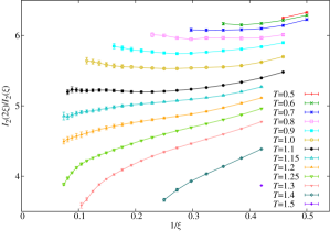
Figure 5: (Color online) For several temperatures, we plot the susceptibility ratio of Eq. (17) as a function of the inverse coherence length.

The crossover implicit in Eq. (17) is shown in Fig. 5, which can be directly compared with Fig. 2 in the main text. One can consider the $\xi\to\infty$ limits in the plot:

• At the critical point $T=T_{\mathrm{c}}$, one expects $2^{2.3900(36)}=5.242(13)$ Baity-Jesi et al. (2013).

• In the spin-glass phase, the droplets model predict a common limit $2^{3}=8$ for all $T<T_{\mathrm{c}}$, while the Replica-Symmetry Breaking theory expects a limit $2^{\theta_{\mathrm{RSB}}}\approx 6.19$.

• The paramagnetic phase is more complicated to discuss. In fact, for $T>T_{\mathrm{c}}$, the coherence length grows only up to its equilibrium value for that temperature, $\xi_{\text{eq}}(T)$. This means that all the (paramagnetic) curves in Fig. 5 have an end point. At this end-point, the longest time $t_{\mathrm{w}}^{(2)}$ correspond to the equilibrium regime (i.e. $\theta_{2}=1$) while the earliest time is still in the non-equilibrium regime. Hence, it is not easy to anticipate the numerical value of the paramagnetic long-time limit, obtained when $\xi_{\text{eq}}(T)$ tends to infinity.

Data in Fig. 5 can be analyzed in exactly the same way we did for the Binder’s parameter [see Eq. (4) and Fig. 3 in the main text]. However, with the susceptibility ratio Eq. (17), errors are one order of magnitude larger. This is why we abandoned this approach.

References

- Cavagna (2009) A. Cavagna, Physics Reports 476, 51 (2009), arXiv:0903.4264 .
- Adam and Gibbs (1965) G. Adam and J. H. Gibbs, J. Chem. Phys. 43, 139 (1965).
- Weeks et al. (2000) E. R. Weeks, J. C. Crocker, A. C. Levitt, A. Schofield, and D. A. Weitz, Science 287, 627 (2000).
- Berthier et al. (2005) L. Berthier, G. Biroli, J.-P. Bouchaud, L. Cipelletti, D. El Masri, D. L’Hôte, F. Ladieu, and M. Pierno, Science 310, 1797 (2005).
- Gutiérrez et al. (2014) R. Gutiérrez, S. Karmakar, Y. G. Pollack, and I. Procaccia, (2014), arXiv:1409.5067 .
- Gunnarsson et al. (1991) K. Gunnarsson, P. Svedlindh, P. Nordblad, L. Lundgren, H. Aruga, and A. Ito, Phys. Rev. B 43, 8199 (1991).
- Palassini and Caracciolo (1999) M. Palassini and S. Caracciolo, Phys. Rev. Lett. 82, 5128 (1999), arXiv:cond-mat/9904246 .
- Ballesteros et al. (2000) H. G. Ballesteros, A. Cruz, L. A. Fernandez, V. Martin-Mayor, J. Pech, J. J. Ruiz-Lorenzo, A. Tarancon, P. Tellez, C. L. Ullod, and C. Ungil, Phys. Rev. B 62, 14237 (2000), arXiv:cond-mat/0006211 .
- Vincent et al. (1997) E. Vincent, J. Hammann, M. Ocio, J.-P. Bouchaud, and L. F. Cugliandolo, in Complex Behavior of Glassy Systems, Lecture Notes in Physics No. 492, edited by M. Rubí and C. Pérez-Vicente (Springer, 1997).
- Bray (1994) A. J. Bray, Adv. Phys. 43, 357 (1994).
- Joh et al. (1999) Y. G. Joh, R. Orbach, G. G. Wood, J. Hammann, and E. Vincent, Phys. Rev. Lett. 82, 438 (1999).
- Bert et al. (2004) F. Bert, V. Dupuis, E. Vincent, J. Hammann, and J.-P. Bouchaud, Phys. Rev. Lett. 92, 167203 (2004).
- Rieger (1993) H. Rieger, J. Phys. A 26, L615 (1993).
- Kisker et al. (1996) J. Kisker, L. Santen, M. Schreckenberg, and H. Rieger, Phys. Rev. B 53, 6418 (1996).
- Marinari et al. (2000a) E. Marinari, G. Parisi, F. Ricci-Tersenghi, J. J. Ruiz-Lorenzo, and F. Zuliani, J. Stat. Phys. 98, 973 (2000a), arXiv:cond-mat/9906076 .
- Marinari et al. (2000b) E. Marinari, G. Parisi, F. Ricci-Tersenghi, and J. J. Ruiz-Lorenzo, J. Phys. A 33, 2373 (2000b).
- Berthier and Bouchaud (2002) L. Berthier and J.-P. Bouchaud, Phys. Rev. B 66, 054404 (2002).
- Berthier and Young (2005) L. Berthier and A. P. Young, Phys. Rev. B 71, 214429 (2005).
- Jaubert et al. (2007) L. C. Jaubert, C. Chamon, L. F. Cugliandolo, and M. Picco, J. Stat. Mech. 2007, P05001 (2007).
- Belletti et al. (2008a) F. Belletti, M. Cotallo, A. Cruz, L. A. Fernandez, A. Gordillo-Guerrero, M. Guidetti, A. Maiorano, F. Mantovani, E. Marinari, V. Martin-Mayor, A. M. Sudupe, D. Navarro, G. Parisi, S. Perez-Gaviro, J. J. Ruiz-Lorenzo, S. F. Schifano, D. Sciretti, A. Tarancon, R. Tripiccione, J. L. Velasco, and D. Yllanes (Janus Collaboration), Phys. Rev. Lett. 101, 157201 (2008a), arXiv:0804.1471 .
- Belletti et al. (2009) F. Belletti, A. Cruz, L. A. Fernandez, A. Gordillo-Guerrero, M. Guidetti, A. Maiorano, F. Mantovani, E. Marinari, V. Martin-Mayor, J. Monforte, A. Muñoz Sudupe, D. Navarro, G. Parisi, S. Perez-Gaviro, J. J. Ruiz-Lorenzo, S. F. Schifano, D. Sciretti, A. Tarancon, R. Tripiccione, and D. Yllanes (Janus Collaboration), J. Stat. Phys. 135, 1121 (2009), arXiv:0811.2864 .
- Manssen and Hartmann (2014) M. Manssen and A. K. Hartmann, (2014), arXiv:1411.5512 .
- Belletti et al. (2008b) F. Belletti, M. Cotallo, A. Cruz, L. A. Fernandez, A. Gordillo, A. Maiorano, F. Mantovani, E. Marinari, V. Martin-Mayor, A. Muñoz Sudupe, D. Navarro, S. Perez-Gaviro, J. J. Ruiz-Lorenzo, S. F. Schifano, D. Sciretti, A. Tarancon, R. Tripiccione, and J. L. Velasco (Janus Collaboration), Comp. Phys. Comm. 178, 208 (2008b), arXiv:0704.3573 .
- Franz et al. (1998) S. Franz, M. Mézard, G. Parisi, and L. Peliti, Phys. Rev. Lett. 81, 1758 (1998).
- Barrat and Berthier (2001) A. Barrat and L. Berthier, Phys. Rev. Lett. 87, 087204 (2001).
- Alvarez Baños et al. (2010) R. Alvarez Baños, A. Cruz, L. A. Fernandez, J. M. Gil-Narvion, A. Gordillo-Guerrero, M. Guidetti, A. Maiorano, F. Mantovani, E. Marinari, V. Martin-Mayor, J. Monforte-Garcia, A. Muñoz Sudupe, D. Navarro, G. Parisi, S. Perez-Gaviro, J. J. Ruiz-Lorenzo, S. F. Schifano, B. Seoane, A. Tarancon, R. Tripiccione, and D. Yllanes (Janus Collaboration), Phys. Rev. Lett. 105, 177202 (2010), arXiv:1003.2943 .
- Jönsson et al. (2002) P. E. Jönsson, H. Yoshino, P. Nordblad, H. Aruga Katori, and A. Ito, Phys. Rev. Lett. 88, 257204 (2002).
- Nakamae et al. (2012) S. Nakamae, C. Crauste-Thibierge, D. L’Hôte, E. Vincent, E. Dubois, V. Dupuis, and R. Perzynski, Appl. Phys. Lett. 101, 242409 (2012).
- Guchhait and Orbach (2014) S. Guchhait and R. Orbach, Phys. Rev. Lett. 112, 126401 (2014).
- Hasenbusch et al. (2008a) M. Hasenbusch, A. Pelissetto, and E. Vicari, J. Stat. Mech. 2008, L02001 (2008a).
- Baity-Jesi et al. (2013) M. Baity-Jesi, R. A. Baños, A. Cruz, L. A. Fernandez, J. M. Gil-Narvion, A. Gordillo-Guerrero, D. Iniguez, A. Maiorano, F. Mantovani, E. Marinari, V. Martin-Mayor, J. Monforte-Garcia, A. Muñoz Sudupe, D. Navarro, G. Parisi, S. Perez-Gaviro, M. Pivanti, F. Ricci-Tersenghi, J. J. Ruiz-Lorenzo, S. F. Schifano, B. Seoane, A. Tarancon, R. Tripiccione, and D. Yllanes (Janus Collaboration), Phys. Rev. B 88, 224416 (2013), arXiv:1310.2910 .
- Ozeki and Ito (2007) Y. Ozeki and N. Ito, J. Phys. A: Math. Theor. 40, R149 (2007).
- Hohenberg and Halperin (1977) P. Hohenberg and B. Halperin, Rev. Mod. Phys. 49, 435 (1977).
- Landau and Binder (2005) D. P. Landau and K. Binder, A Guide to Monte Carlo Simulations in Statistical Physics, 2nd ed. (Cambridge University Press, Cambridge, 2005).
- Lulli et al. (2014a) M. Lulli, M. Bernaschi, and G. Parisi, “Highly optimized simulations on single- and multi-gpu systems of 3d ising spin glass,” (2014a), in preparation, arXiv:1411.0127 .
- Fang et al. (2014) Y. Fang, S. Feng, K.-M. Tam, Z. Yun, J. Moreno, J. Ramanujam, and M. Jarrell, Comp. Phys. Comm. 185, 2467– (2014), arXiv:1311.5582 .
- Feng et al. (2014) S. Feng, Y. Fang, K.-M. Tam, Z. Yun, J. Ramanujam, J. Moreno, and M. Jarrell, (2014), arXiv:1403.4560 .
- Gillespie (1977) D. T. Gillespie, J. Phys. Chem. 81, 2340 (1977).
- Bortz et al. (1975) A. B. Bortz, M. H. Kalos, and J. L. Lebowitz, J. Comp. Phys. 17, 10 (1975).
- Bouchaud et al. (2001) J.-P. Bouchaud, V. Dupuis, J. Hammann, and E. Vincent, Phys. Rev. B 65, 024439 (2001).
- Liu et al. (2014) C.-W. Liu, A. Polkovnikov, A. Sandvik, and A. P. Young, (2014), arXiv:1411.6745 .
- Nightingale and Blöte (2000) M. Nightingale and H. Blöte, Phys. Rev. B 62, 1089 (2000).
- Mydosh (1993) J. A. Mydosh, Spin Glasses: an Experimental Introduction (Taylor and Francis, London, 1993).
- Nakamura et al. (2003) T. Nakamura, S.-i. Endoh, and T. Yamamoto, J. Phys. A 36, 10895 (2003).
- Romá (2010) F. Romá, Phys. Rev. B 82, 212402 (2010).
- Binder (1981) K. Binder, Z. Phys. B – Condensed Matter 43, 119 (1981).
- Nakamura (2010) T. Nakamura, Phys. Rev. B 82, 014427 (2010).
- Marinari et al. (1996) E. Marinari, G. Parisi, J. Ruiz-Lorenzo, and F. Ritort, Phys. Rev. Lett. 76, 843 (1996).
- Amit and Martin-Mayor (2005) D. J. Amit and V. Martin-Mayor, Field Theory, the Renormalization Group and Critical Phenomena, 3rd ed. (World Scientific, Singapore, 2005).
- Parisi (1988) G. Parisi, Statistical Field Theory (Addison-Wesley, 1988).
- Marinari et al. (1998) E. Marinari, G. Parisi, F. Ricci-Tersenghi, and J. J. Ruiz-Lorenzo, Journal of Physics A: Math. and Gen. 31, L481 (1998).
- Newman and Stein (1998) C. M. Newman and D. L. Stein, Phys. Rev. E 57, 1356 (1998).
- Hasenbusch et al. (2008b) M. Hasenbusch, A. Pelissetto, and E. Vicari, Phys. Rev. B 78, 214205 (2008b).
- Baños et al. (2012a) R. A. Baños, A. Cruz, L. A. Fernandez, J. M. Gil-Narvion, A. Gordillo-Guerrero, M. Guidetti, D. Iniguez, A. Maiorano, E. Marinari, V. Martin-Mayor, J. Monforte-Garcia, A. Muñoz Sudupe, D. Navarro, G. Parisi, S. Perez-Gaviro, J. J. Ruiz-Lorenzo, S. F. Schifano, B. Seoane, A. Tarancon, P. Tellez, R. Tripiccione, and D. Yllanes, Proc. Natl. Acad. Sci. USA 109, 6452 (2012a).
- Baity-Jesi et al. (2014) M. Baity-Jesi, L. A. Fernandez, V. Martin-Mayor, and J. M. Sanz, Phys. Rev. 89, 014202 (2014), arXiv:1309.1599 .
- Bouchiat (1986) H. Bouchiat, J. Phys. France 47, 71 (1986).
- Lévy (1988) L. P. Lévy, Phys. Rev. B 38, 4963 (1988).
- Petit et al. (2002) D. Petit, L. Fruchter, and I. A. Campbell, Phys. Rev. Lett 88, 207206 (2002), arXiv:cond-mat/011112 .
- Campbell and Petit (2010) I. A. Campbell and D. C. M. C. Petit, J. Phys. Soc. Jpn. 79, 011006 (2010), arXiv:0907.5333 .
- Mari and Campbell (1999) P. Mari and I. Campbell, Phys. Rev. E 59, 2653 (1999).
- Pleimling and Campbell (2005) M. Pleimling and I. Campbell, Phys. Rev. B 72, 184429 (2005).
- Lulli et al. (2014b) M. Lulli, G. Parisi, and A. Pelissetto, “Out-of-equilibrium measure of critical parameters for second-order phase transitions,” (2014b), in preparation.
- Oukris and Israeloff (2010) H. Oukris and N. E. Israeloff, Nature Physics 06, 135 (2010).
- Komatsu et al. (2011) K. Komatsu, D. L’Hôte, S. Nakamae, V. Mosser, M. Konczykowski, E. Dubois, V. Dupuis, and R. Perzynski, Phys. Rev. Lett. 106, 150603 (2011), arXiv:1010.4012 .
- Rodriguez et al. (2003) G. F. Rodriguez, G. G. Kenning, and R. Orbach, Phys. Rev. Lett. 91, 037203 (2003).
- Rodriguez et al. (2013) G. Rodriguez, G. Kenning, and R. Orbach, Phys. Rev. B 88, 054302 (2013).
- Newman and Barkema (1999) M. E. J. Newman and G. T. Barkema, Monte Carlo Methods in Statistical Physics (Clarendon Press, Oxford, 1999).
- Leuzzi et al. (2008) L. Leuzzi, G. Parisi, F. Ricci-Tersenghi, and J. J. Ruiz-Lorenzo, Phys. Rev. Lett. 101, 107203 (2008).
- Baños et al. (2012b) R. A. Baños, L. A. Fernandez, V. Martin-Mayor, and A. P. Young, Phys. Rev. B 86, 134416 (2012b), arXiv:1207.7014 .
- Fernandez et al. (2010) L. A. Fernandez, V. Martin-Mayor, G. Parisi, and B. Seoane, Phys. Rev. B 81, 134403 (2010).
- Hukushima and Nemoto (1996) K. Hukushima and K. Nemoto, J. Phys. Soc. Japan 65, 1604 (1996), arXiv:cond-mat/9512035 .
- Marinari (1998) E. Marinari, in Advances in Computer Simulation, edited by J. Kerstész and I. Kondor (Springer-Verlag, 1998).
- McMillan (1984) W. L. McMillan, J. Phys. C: Solid State Phys. 17, 3179 (1984).
- Bray and Moore (1987) A. J. Bray and M. A. Moore, in Heidelberg Colloquium on Glassy Dynamics, Lecture Notes in Physics No. 275, edited by J. L. van Hemmen and I. Morgenstern (Springer, Berlin, 1987).
- Fisher and Huse (1986) D. S. Fisher and D. A. Huse, Phys. Rev. Lett. 56, 1601 (1986).
- Fisher and Huse (1988) D. S. Fisher and D. A. Huse, Phys. Rev. B 38, 386 (1988).