Made–to–Measure Dark Matter Haloes, Elliptical Galaxies and Dwarf Galaxies in Action Coordinates

Abstract

We provide a family of action-based distribution functions (DFs) for the double–power law family of densities often used to model galaxies. The DF itself is a double–power law in combinations of the actions, and reduces to the pure power–law case at small and large radii. Our method enables the velocity anisotropy of the model to be tuned, and so the anisotropy in the inner and outer parts can be specified for the application in hand. We provide self-consistent DFs for the Hernquist and Jaffe models – both with everywhere isotropic velocity dispersions, and with kinematics that gradually become more radially anisotropic on moving outwards. We also carry out this exercise for a cored dark–matter model. These are tailored to represent dark haloes and elliptical galaxies respectively with kinematic properties inferred from simulations or observational data. Finally, we relax a cored luminous component within a dark matter halo to provide a self-consistent model of a dwarf spheroidal embedded in dark matter. The DFs provide us with non-rotating spherical stellar systems, but one of the virtues of working with actions is the relative ease with which such models can be converted into axisymmetry and triaxiality.

1 INTRODUCTION

The interpretation of kinematic observations of galaxies in terms of their orbital structure is an important and difficult problem in modern-day galaxy dynamics. For external galaxies, the kinematics may include mean motions, velocity dispersions and even line profiles, or the entire distribution of line of sight velocities. For the Milky Way, the problem has been given additional impetus by the advent of large-scale spectroscopic surveys, together with the launch of the Gaia satellite, which will provide discrete velocities on about a billion objects (e.g., Perryman et al. 2001). Moment based methods, such as the Jeans equations, offer a simple and widely used method for reproducing the density and velocity dispersion (e.g., Fillmore 1986). Nonetheless, they are much less powerful than distribution function (or DF) based methods, which can directly fit not just mere moments, but also the distributions of kinematical quantities (e.g., Wojtak & Łokas 2010; Amorisco & Evans 2011; Wojtak & Mamon 2013; Strigari et al. 2014).

However, construction of equilibrium DFs for galaxies is far from easy. There do exist numerical algorithms such as Schwarzschild’s (1979) orbit superposition method or Syer & Tremaine’s (1996) made-to-measure method. These can be thought of as ways to fit orbits or N-body models to kinematic data, such that the deviation of moments from the observables are minimized subject to some penalty function that enforces smoothness. Schwarzschild’s method, at least in its axisymmetric implementation, has proved invaluable in the analysis of integral-field stellar kinematics on elliptical galaxies (e.g., Cappellari et al. 2007). The made-to-measure method has also been applied to elliptical galaxies to assess their dark matter content and orbital anisotropy (de Lorenzi et al., 2008).

There also exist classes of simple analytic DFs, though these are restricted to spherical symmetry or to axisymmetry (e.g., Dejonghe 1986). DFs can only depend on the isolating integrals of motion by Jeans (1919) theorem. In spherical potentials, they are the energy $E$ and angular momentum components $\mn@boldsymbol{L}$; in axisymmetric potentials, they are energy $E$ and component of angular momentum parallel to the symmetry axis $L_{z}$. Given the density, general algorithms exists to find smooth DFs based on the classical integrals (Eddington 1915, Hunter & Qian 1993, Evans & An 2006). There also systems with known DFs, including power-laws (Evans, 1994) and double power-laws, such as Hernquist (1990) and Jaffe (1983) models.

Binney (2008) has argued that it is more natural to use actions as the choice of integrals of motion rather than classical integrals, such as energy. This is partly because the actions are adiabatic invariants, and partly because action-based DFs can be more easily generalized to flattened and triaxial geometries. Binney (2010, 2012) provided a significant advance when he showed that the data on the thin disk of the Milky Way can be largely accounted for by models synthesised from quasi-isothermal DFs. The thin disk provides a particularly clean application for two reasons. First, the stellar orbits are close to circular and so the actions of stars are readily computed in terms of epicyclic theory and its extensions. Second, the quasi-isothermal assumption provides a simple and physically motivated ansatz for the DF, building on earlier ideas that the DF is Maxwellian about the circular speed (Shu, 1967).

The purpose of this paper is to extend this work to hotter, or pressure-supported, stellar systems. That is, we seek similar action-based DFs for elliptical galaxies or bulges or haloes. Ideally, the DFs should be tunable, so that the user may specify the power-law fall-off in the density at large and small radii, as well as properties of the velocity anisotropy at large and small radii. Such an algorithm provides the user with a way of making made-to-measure haloes or elliptical galaxies.

2 Background

Here, we introduce some important concepts relating to this work that will prove important in the main body of the paper. First, we describe how to compute a self–consistent model given an action–based distribution function. Then,we describe how to construct constant anisotropy DFs for simple power–law models.

2.1 Computing a Self–Consistent Model

Action integrals are adiabatically invariant, which means that slow changes in $\Phi(r)$ do not alter ${\boldsymbol{J}}$. By extension, an action–based distribution function $f({\boldsymbol{J}})$ is also adiabatically invariant. This allows us to propose a model $f({\boldsymbol{J}})$ and iteratively converge upon its corresponding potential, $\Phi_{f}$, from an initial educated guess $\Phi_{0}$. In a spherical system, the relevant actions are the azimuthal action $J_{\phi}=L_{z}$, the vertical action $J_{\theta}=L-|L_{z}|$, and the radial action

$$J_{r}=\dfrac{1}{2\pi}\oint\sqrt{-2E-2\Phi(r)-L^{2}/r^{2}}\mathrm{d}r.$$ (1)

However, for a non–rotating spherical system, one can show that the Hamiltonian (and hence the DF) can be written as a function of just $L=J_{\theta}+|J_{\phi}|$ and $J_{r}$. We thus write $f({\boldsymbol{J}})=f(L,J_{r})$. The algorithm to find the self–consistent model is as follows (Binney & Tremaine, 2008)

1. From the initial guess potential, $\Phi_{0}$, compute the radial action $J_{r}({\boldsymbol{x}},{\boldsymbol{v}})$ as a function of the phase–space coordinates (the other action, $L$, is potential–independent).

2. Compute the implied density profile of $f({\boldsymbol{J}})$ under $\Phi_{0}$ by carrying out the integral

   $$\rho_{1}({\boldsymbol{x}})=\int{\mathrm{d}}^{3}{\boldsymbol{v}}f\left(L({\boldsymbol{x}},{\boldsymbol{v}}),J_{r}({\boldsymbol{x}},{\boldsymbol{v}})\right).$$ (2)

3. Solve Poisson’s equation to find the potential implied by $\rho_{1}$

   $${\vec{\nabla}}^{2}\Phi_{1}({\boldsymbol{x}})=4\pi G\rho_{1}({\boldsymbol{x}}).$$ (3)

4. Repeat steps (i) $\rightarrow$ (iii) with $\Phi_{1}$ in place of $\Phi_{0}$ and compute $\Phi_{2}$.

5. Iterate until the difference between $\Phi_{i}$ and $\Phi_{i+1}$ is negligible.

Once the algorithm has converged, and we possess $\Phi_{f}$, we can compute the radial action (and therefore DF) as a function of the phase–space coordinates $({\boldsymbol{x}},{\boldsymbol{v}})$. This means that we can compute any observable we choose in a self–consistent fashion. The adiabatic invariance of $f({\boldsymbol{J}})$ means that we can create models composed of many different components (e.g. galaxy models with a dark halo, disk and bulge) and relax them simultaneously. It is this unique feature of $f({\boldsymbol{J}})$ models that makes them so useful.

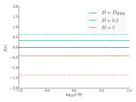
Figure 1: Anisotropy profiles for potentials with $\Phi\propto r^{\pm 1/2}$. Solid lines correspond to models where $\epsilon=1/2$ and dashed lines to $\epsilon=-1/2$. $D_{\mathrm{WEB}}$ is obtained from Equation (7), giving very nearly isotropic models, $D=0.2$ creates radially biased models and $D=5$ creates tangentially biased models. All the models have constant anisotropy, as predicted.

2.2 Power–Law Models

Before we derive DFs for more complex models, it is instructive to consider the simpler task of constructing distribution functions for a power–law model with density law:

$$\rho(r)=\rho_{0}\left(\dfrac{r}{a}\right)^{-\nu}.$$ (4)

Such a density distribution will generate a gravitational potential $\Phi(r)\propto r^{\epsilon}$, where $\epsilon=2-\nu$. We can then construct isotropic distribution functions for these systems as a function of binding energy (Evans, 1994)

$$f(E)\propto|E|^{-\dfrac{\epsilon+4}{2\epsilon}}.$$ (5)

An obvious way to obtain a distribution function in action space is to then express the binding energy (given by $E=-H$, where $H$ is the Hamiltonian) as a function of the actions ${\boldsymbol{J}}$, and substitute the resulting expression into Equation (5). Williams, Evans & Bowden (2014) (hereafter WEB) provide an approximation to the Hamiltonians of power–law models, given by

$$\mathcal{H}({\boldsymbol{J}})\propto(L+DJ_{r})^{\zeta},$$ (6)

where $\zeta=2\epsilon/(\epsilon+2)$ and

$$D=\begin{cases}\dfrac{\sqrt{2\pi}\Gamma(3/2+1/\epsilon)\epsilon^{-1/\epsilon}\zeta^{1/\zeta}}{\Gamma(1+1/\epsilon)}&\epsilon>0\\ \sqrt{2\mathrm{\pi}/e}&\epsilon=0\vspace{6pt}\\ \dfrac{\sqrt{2\pi}\Gamma(1-1/\epsilon)(-\epsilon)^{1-1/\epsilon}(-\zeta)^{1/\zeta}}{\Gamma(-1/\epsilon-1/2)}&\epsilon<0.\\ \end{cases}$$ (7)

Given Equation (6), the distribution function in action–space is given by

$$f({\boldsymbol{J}})\propto(L+DJ_{r})^{-(\epsilon+4)/(\epsilon+2)}.$$ (8)

This expression is therefore an approximate isotropic distribution function for the power law in Equation (4) when $0\leq\nu<3$. We note that Equation (8) still holds in the case $\nu=2$ and the potential is logarithmic. We now turn to the problem of constructing constant anisotropy power–law models. The anisotropy parameter is given by

$$\beta(r)=1-\dfrac{\sigma^{2}_{t}(r)}{2\sigma^{2}_{r}(r)},$$ (9)

where $\sigma_{r}$/$\sigma_{t}$ are the radial/tangential velocity dispersions. $\beta$ quantifies the relative importance of radial and tangential orbits at radius $r$: when a model is completely constructed from radial/circular orbits $\beta\rightarrow 1/-\infty$. To construct constant anisotropy power–laws, we can take the commonly used ansatz (e.g., Wilkinson & Evans 1999, Evans & An 2006, Deason, Belokurov & Evans 2011)

$$f(E,L)=L^{-2\beta}g(E),$$ (10)

and once again substitute for $E$ using Equation (6). However, we can also note that a density profile with the same radial dependence as Equation (4) is generated by any non–negative, scale–free DF with the dimensions of Equation (8). As a consequence, we can construct a family of constant anisotropy power laws using a DF of the form of Equation (8). When $\nu$ is fixed, the isotropic model belonging to this family is generated when the parameter $D$ is set equal to the value implied by Equation (7), and anisotropic models can be generated by altering the value of this parameter. The anisotropy profile must be constant with radius for all such models, as they possess no scale. We can intuitively understand how different values of $D$ will produce different anisotropies. $D$ controls the relative importance of tangential and radial orbits: a model that more heavily weights the angular momentum will become tangentially biased, whereas favouring the radial action will result in radial bias. Since the DF is a declining function of ${\boldsymbol{J}}$, we can expect that an increase in $D$ from the WEB value of Equation (7) will produce a tangentially biased model, and a decrease will result in a radially biased model.

As an example, Figure 1 depicts the variation in the anisotropy parameter for three choices of $D$ in the cases $\epsilon=\pm 1/2$. The three different values are $D_{\mathrm{WEB}}$ from Equation (7), 0.2 and 5. $D_{\mathrm{WEB}}$ produces very nearly isotropic models, $D=5$ creates tangentially biased models and $D=0.2$ creates radially biased models. All the models have constant anisotropy as expected.

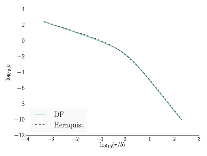
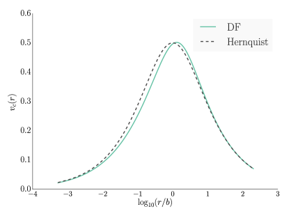
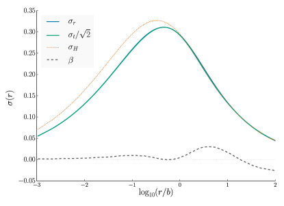
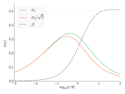
Figure 2: Top row: comparison of the density (left) and circular speed (right) profiles generated by the DF (28) and the Hernquist model. The densities are in excellent agreement, and the circular speed curves match well, other than a mild offset visible at small radii. Bottom row: the kinematics of the two dark matter models. The model intended to be isotropic (left) is almost so, with $\beta$ only fluctuating on scales of $\sim 0.01$. The dotted line depicts the isotropic velocity dispersion of the equivalent isotropic Hernquist model ($\sigma_{H}$), which agrees well with our models other than a small offset in the cusp of the model. The radially distended model (right) moves smoothly from $\beta_{0}=0$ to $\beta_{1}=0.5$ across a scale of $r_{\beta}=b$. We set $G=M=b=1$ for these models.

3 Double–Power law DF

Having deduced how to produce constant anisotropy power–law distribution functions, we now aim to extend this reasoning to construct a family of distribution functions that will generate double power–law density profiles (see e.g. Binney & Tremaine 2008):

$$\rho(r)=\dfrac{\rho_{0}b^{\gamma}}{r^{\alpha}(b+r)^{\gamma-\alpha}}.$$ (11)

We restrict ourselves to finite–mass models in this case, i.e. $\gamma>3$. Such a density profile breaks around the radius $r=b$, behaving as $r^{-\alpha}$ when $r\ll b$ and as $r^{-\gamma}$ when $r\gg b$. It is by consideration of these power–law limits, in combination with the reasoning from Section 2.2, that will allow us to construct a suitable DF to emulate the density profile of Equation (11). In what follows, we shall derive our distribution function designed to mimic these models, then describe how to tune the anisotropy parameter.

3.1 Derivation of the DF

Consider the isotropic distribution function of the double power–law models, $f(E)$: even if we cannot explicitly calculate its functional form everywhere, we can infer what it should look like in the limits of high/low binding energy. At high binding energies, the overwhelming contribution to the density profile will come from orbits that reside at radii $r\ll b$. As a result, the DF will resemble that of a power–law model with density $\rho\sim r^{-\alpha}$, with the same form as Equation (8).

At low binding energies orbits reside in a Keplerian potential, owing to the assumed finite mass of the model. In this case, we turn to Eddington’s equation to discover the behaviour of $f(E)$:

$$f(E)\propto\dfrac{{\mathrm{d}}}{{\mathrm{d}}E}\int^{E}_{0}\dfrac{{\mathrm{d}}\Psi}{\sqrt{E-\Psi}}\dfrac{{\mathrm{d}}\rho}{{\mathrm{d}}\Psi},$$ (12)

where $\Psi=-\Phi$ is the relative potential. In this case, we have that $\rho\propto\Psi^{\gamma}$, and Eddington’s equation may be solved to give

$$f(E)\propto E^{\gamma-\frac{3}{2}}.$$ (13)

An expression for $E$ in terms of ${\boldsymbol{J}}$ is now required. At low binding energies the Hamiltonian coincides with the Kepler case (e.g., Goldstein 1980)

$$H({\boldsymbol{J}})=\dfrac{-(GM)^{2}}{2\left(L+J_{r}\right)^{2}},$$ (14)

where $M$ is the mass of the model. We have thus discovered the limiting behaviour of $f({\boldsymbol{J}})$ to be

$$f({\boldsymbol{J}})=\begin{cases}S_{\alpha}(L+D_{\alpha}J_{r})^{(\alpha-6)/(4-\alpha)}&E\ll-\Phi(b)\\ S_{\gamma}(L+J_{r})^{-2\gamma+3}&E\gg-\Phi(b),\end{cases}$$ (15)

where $S_{\alpha}$ and $S_{\gamma}$ are constants, and $D_{\alpha}$ is given by Equation (7) with $\alpha=\nu$. We must now construct a full DF that satisfies these limits, whilst also recovering sensible behaviour in–between. Given that the density law itself is a double power–law, a simple first guess at an appropriate functional form is a double power–law in the actions. Hence, we choose the following DF:

$$f({\boldsymbol{J}})=\dfrac{\mathcal{N}\,M}{(2\mathrm{\pi})^{3}J_{0}^{3-\mu}}\,\dfrac{T({\boldsymbol{J}})\,\mathcal{L}({\boldsymbol{J}})^{-\lambda}}{\left[J_{0}^{2}+\mathcal{L}({\boldsymbol{J}})^{2}\right]^{(\mu-\lambda)/2}},$$ (16)

where we have set $\lambda=(6-\alpha)/(4-\alpha)$, $\mu=2\gamma-3$ and

$$\mathcal{L}({\boldsymbol{J}}) = L+D({\boldsymbol{J}})J_{r}$$

$$D({\boldsymbol{J}}) = \dfrac{D_{0}+D_{1}|{\boldsymbol{J}}|/J_{\beta}}{1+|{\boldsymbol{J}}|/J_{\beta}}.$$ (17)

$$T({\boldsymbol{J}}) = \dfrac{S_{\alpha}+S_{\gamma}|{\boldsymbol{J}}|/J_{0}}{1+|{\boldsymbol{J}}|/J_{0}}$$

$$|{\boldsymbol{J}}| = \sqrt{L^{2}+J_{r}^{2}}$$

Several of the components in this DF require explanation. The natural action scale of the model is

$$J_{0}=\sqrt{GMb},$$ (18)

and controls the transition from one power–law regime to the other. The argument $\mathcal{L}({\boldsymbol{J}})$ is inspired by the linearity of the Hamiltonian of the model in the two limits. However, the planes in ${\boldsymbol{J}}$–space upon which the DF is stratified change with growing ${\boldsymbol{J}}$, as the model passes between the two regimes. This change is facilitated by the function $D({\boldsymbol{J}})$. The number $D_{0}$/$D_{1}$ quantifies the slope of these planes at high/low binding energies (small/large action), and $D({\boldsymbol{J}})$ transits $D_{0}\rightarrow D_{1}$ over the action scale $J_{\beta}$. For the ergodic case, $D_{0}$ can be found analytically using Equation (7) and $D_{1}=1$. The action scale $J_{\beta}$ differs from the natural action scale, and will help us to construct models with made–to–measure kinematics. This will be explained in detail shortly.

In general $f(E)$ is not a double–power law in energy, but is usually rather more complicated. For some models (e.g. Hernquist 1990, Dehnen 1993, Tremaine et al. 1994) $f(E)$ can be computed wholly analytically, and the added complexity becomes transparent. However, Equation (16) assumes that $f(E)$ can be approximated by interpolating between the limiting cases as a double–power law. If we are to do this effectively, we must ensure that the limiting cases we sew together have the correct relative normalisation. This amounts to computing the constant factors $S_{\alpha}$ and $S_{\gamma}$ in Equation (15), so that $f({\boldsymbol{J}})$ coincides exactly with the correct limits. $T({\boldsymbol{J}})$ fulfills this purpose by acting as a “variable normalisation” of the DF, interpolating between $S_{\alpha}$ and $S_{\gamma}$ over the action scale of the model. For many models (even if $f(E)$ cannot be represented by elementary functions) $S_{\alpha}$ and $S_{\gamma}$ can be computed analytically. See Appendix A for a derivation of these quantities in the case $\gamma=4$.

Finally, the normalisation factor $\mathcal{N}$ ensures that the DF integrates to the correct mass:

$$M=(2\pi)^{3}\int{\mathrm{d}}^{3}{\boldsymbol{J}}f({\boldsymbol{J}})$$ (19)

and is computed by a swift numerical integration.

3.2 Tuning the Anisotropy Profile

Here, we describe an algorithm to tailor the anisotropy of a model. We can use the logic found in Section 2.2 to tune the anisotropy of our models in the central/far–field regimes. Using Equation (3.1), in the limit $|{\boldsymbol{J}}|\ll J_{\beta}$, we find that $D\rightarrow D_{0}$. In the opposite limit, $D\rightarrow D_{1}$. The action scale $J_{\beta}$ controls the speed at which we transit from one limit to the other. This allows us to vary $D_{0}$ until we reach the desired inner anisotropy $\beta_{0}$, then independently vary $D_{1}$ until the outer anisotropy is some value $\beta_{1}$. Once the values of $D_{0}$ and $D_{1}$ are fixed, we can vary how fast the model transits from $\beta_{0}$ to $\beta_{1}$ by altering the value of $J_{\beta}$.

An important subtlety of this procedure is that the relative normalisation factor $T({\boldsymbol{J}})$ must change as a consequence. Consider the value of the DF at some point in action space ${\boldsymbol{J}}=J_{L}(1,1)$ where $J_{L}$ is large. Before the transformation of $D_{1}$ (we begin with $D_{1}=1$, the isotropic value), this is equal to

$$f({\boldsymbol{J}})=\mathcal{N}S_{\gamma}(2J_{L})^{-\mu}.$$ (20)

After changing $D_{1}$, this becomes

$$f^{\prime}({\boldsymbol{J}})=\mathcal{N}S_{\gamma}\left[(1+D_{1})J_{L}\right]^{-\mu}.$$ (21)

Thus the weight of the DF at this point in action space has changed by a factor

$$\Delta f=\left(\dfrac{1+D_{1}}{2}\right)^{-\mu}.$$ (22)

This suggests we make the transformation

$$S_{\gamma}\rightarrow S_{\gamma}\left(\dfrac{2}{1+D_{1}}\right)^{-\mu}$$ (23)

in order to preserve the weight of the DF in the far–field. Similar logic applies in the center of the model, leading to the transformation

$$S_{\alpha}\rightarrow S_{\alpha}\left(\dfrac{1+D_{\mathrm{WEB}}}{1+D_{0}}\right)^{-\lambda}$$ (24)

where $D_{\mathrm{WEB}}$ is the isotropic value from Equation (7). After these transformations, the density profile should barely be altered as a consequence of the anisotropy tuning. Our algorithm is then as follows:

1. Choose a central anisotropy, $\beta_{0}$ and a far–field anisotropy $\beta_{1}$. In addition, specify a length scale $r_{\beta}$ over which the anisotropy parameter $\beta(r)$ should transit between these values.

2. Compute the self–consistent isotropic model with $D_{0}$ = $D_{\mathrm{WEB}}$, $D_{1}=1$ and $J_{\beta}=1$.

3. Iteratively compute $D_{0}$ by recalculating $\beta(r_{\mathrm{inner}})$ repeatedly until $\beta(r_{\mathrm{inner}})=\beta_{0}$, where $r_{\mathrm{inner}}\ll r_{\beta}$.

4. Iteratively compute $D_{1}$ by recalculating $\beta(r_{\mathrm{outer}})$ repeatedly until $\beta(r_{\mathrm{outer}})=\beta_{1}$, where $r_{\mathrm{outer}}\gg r_{\beta}$.

5. Minimise the function $|\beta(r_{\beta})-\frac{1}{2}(\beta_{0}+\beta_{1})|$ at fixed $D_{0}$, $D_{1}$ to constrain $J_{\beta}$.

6. Make the transformations from Equations (23) and (24) to minimise changes to the density profile of the model.

If $\beta_{0}=\beta_{1}=0$ then $D_{0}$ and $D_{1}$ are both known analytically. In this case, only step (v) of the algorithm is applied, and serves to minimise fluctuations in $\beta(r)$ across all radii.

4 Applications

Here, we use the DF (16) to generate some self–consistent model galaxies. First we consider a Hernquist–like DF ($\alpha=1$, $\gamma=4$) as a suitable model for a cuspy dark–matter halo. We then compute the cored equivalent to this model ($\alpha=0$, $\gamma=4$). Finally, we investigate a Jaffe–like model ($\alpha=2$, $\gamma=4$) to represent an elliptical galaxy.

To investigate these DFs, we implemented the algorithms of Sections 2.1 and 3.2 in Python. Given a radial grid and an initial guess potential $\Phi_{0}$, our code will provide a self–consistent model with the spatial and kinematic properties readily evaluated. The initial guess potential used in each case is the potential of the target double power–law density distribution (see Appendix A). At each iteration, we make a grid of the radial action as a function of binding energy and angular momentum, $J_{r}(E,L)$. Between gridpoints, we use cubic spline interpolation to find $J_{r}$. Beyond the end of the energy grid (low binding energies) we use the Keplerian approximation for the radial action from Equation (14):

$$J_{r}(E<E_{\mathrm{min}})\simeq\dfrac{GM}{\sqrt{2E}}-L$$ (25)

since we are only considering finite–mass models. Once the radial action grid has been calculated, we numerically integrate the DF to find the new density and potential. After the first iteration, the potential is purely numerical, and is only explicitly calculated at the radial grid–points. We again use cubic spline interpolation to evaluate the potential between grid–points. Beyond the final grid–point, we extrapolate the potential in a Keplerian fashion

$$\Phi(r>r_{\mathrm{max}})=\Phi(r_{\mathrm{max}})\dfrac{r_{\mathrm{max}}}{r}.$$ (26)

Our condition for convergence is that the change in the potential must be $<1\%$ at all the radial gridpoints. To speed convergence, we use the trick employed by Binney (1982, 2014)

$$\Phi_{i+1}=(1+\kappa)\Phi_{i,1/2}-\kappa\Phi_{i}$$ (27)

where $\Phi_{i,1/2}$ is the potential computed by solving Poisson’s equation for the new density profile and $\Phi_{i}$ is the potential from the previous iteration. We find $\kappa=0.5$ is a reasonable value here, and our code converges in $\sim 3$ iterations. In order to test this code, we provided $f({\boldsymbol{J}})$ for the isochrone model (Henon, 1959), which is known entirely analytically, and set $\Phi_{0}$ to the Plummer (1911) potential. Upon convergence, the code recovers the isochrone potential to great accuracy, with the largest error $\sim 1\%$ in the very center of the model. This is not surprising, since our radial grid cannot extend to zero and so the integration to find the potential at the innermost grid–point must rely on extrapolation.

To implement the algorithm of Section 3.2 we used Brent’s method (e.g. Press et al. 2007) to fix the anisotropies at the innermost and outermost grid–points on our radial grid, and the action scale of the anisotropy $J_{\beta}$. This is done after the self–consistent potential and density of the model are found using $D_{0}$ from Equation (7), $D_{1}=1$ and $J_{\beta}=J_{0}$. The DF is then slightly different once $J_{\beta}$, $D_{0}$ and $D_{1}$ are fixed, even after the transformations of Equations (23) and (24) have been applied. If the potential has changed by more than 1% at any of our gridpoints, it is iterated again until our convergence criterion is met. Typically this takes 1 or 2 iterations.

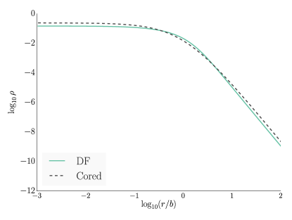
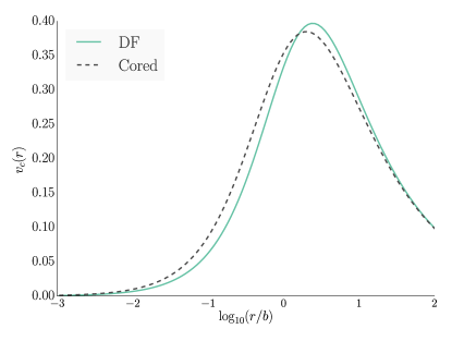
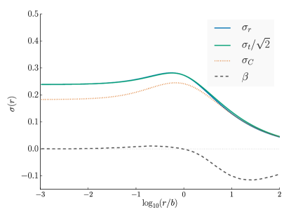
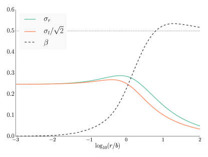
Figure 3: Top row: comparison of the density (left) and circular speed (right) profiles generated by the DF (33) and the cored model. The densities are in good agreement, though less so than for the other models considered here. The DF appears to produce a sharper break than the target density profile, and this is reflected in the circular speed curves. Bottom row: the kinematics of the two cored dark matter models. The isotropic model (left) becomes very mildly tangentially distended with $\beta\sim-0.1$. The dotted line depicts the velocity dispersion profile of the equivalent isotropic cored model ($\sigma_{C}$), which is in good agreement with our DF beyond $r=b$, but offset in the core of the model. The radially distended model (right) switches smoothly from $\beta_{0}=0$ to $\beta_{1}=0.5$ across a scale of $r_{\beta}=b$. We set $G=M=b=1$ for these models.

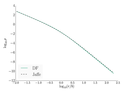
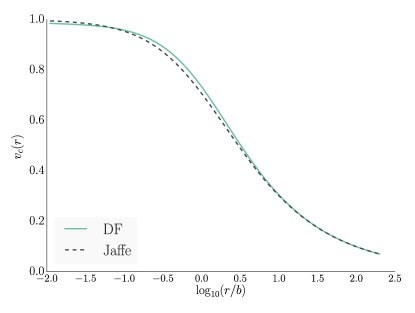
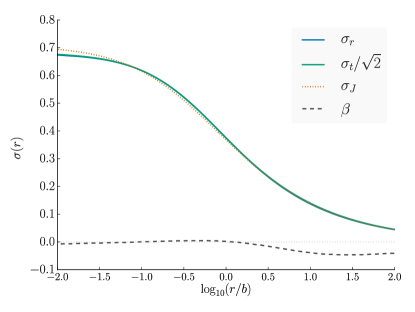
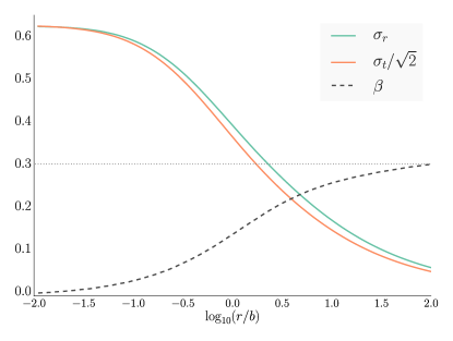
Figure 4: Top row: comparison of the density (left) and circular speed (right) profiles generated by the DF (36) and the Jaffe model. Both the density and the circular speed are in very good agreement. Bottom row: the kinematics of the two elliptical galaxy models. The model intended to be isotropic (left) becomes very mildly tangentially anisotropic in the far–field, with $\beta\sim-0.05$. The dotted line depicts the velocity dispersion profile of the equivalent Jaffe model ($\sigma_{J}$), which matches our model satisfyingly well. The radially anisotropic model (right) switches from $\beta_{0}=0$ to $\beta_{1}=0.3$ across a scale of $r_{\beta}=b$. We set $G=M=b=1$ for these models.

4.1 Dark–Matter DFs

Here, we investigate two appropriate DFs for dark matter haloes. One is cuspy, the other cored. In both cases, we first investigate an isotropic model and then construct a model with more complicated kinematics using anisotropy tuning.

4.1.1 Cuspy Dark Halo

Cuspy dark matter haloes are often modelled using the Hernquist (1990) sphere (e.g. Jang-Condell & Hernquist 2001), a double power–law with $\alpha=1$ and $\gamma=4$. In this case, our DF becomes

$$f({\boldsymbol{J}})=\dfrac{\mathcal{N}\,MJ_{0}^{2}}{(2\mathrm{\pi})^{3}}\,\dfrac{T({\boldsymbol{J}})\,\mathcal{L}({\boldsymbol{J}})^{-5/3}}{\left[J_{0}^{2}+\mathcal{L}({\boldsymbol{J}})^{2}\right]^{5/3}}.$$ (28)

We first consider an isotropic model, where the variable normalisation factor is calculated to be (see Appendix A)

$$T({\boldsymbol{J}})=\dfrac{0.378+|{\boldsymbol{J}}|/J_{0}}{1+|{\boldsymbol{J}}|/J_{0}}$$ (29)

and the weighting factor for the actions is

$$D({\boldsymbol{J}})=\dfrac{\mathrm{\pi}/\sqrt{3}+|{\boldsymbol{J}}|/J_{\beta}}{1+|{\boldsymbol{J}}|/J_{\beta}}$$ (30)

After solving for the self–consistent model, we optimized $J_{\beta}$ using our anisotropy tuning algorithm and found $J_{\beta}=0.41J_{0}$. The two upper panels of Figure 2 depict the comparison of the radial density and circular speed profiles of this model with the Hernquist model of equivalent mass and scale–length. We find that the DF is in excellent agreement with the Hernquist model, the only noticeable discrepancy being a slight offset in the circular speed at small radii. The lower–left panel of Figure 2 depicts the kinematic properties of this model after anisotropy tuning has taken place. Our intention, in this case, was to produce a model as close to isotropic as possible. We can see that this target has been well–met, with $\beta$ only fluctuating on scales $\sim 0.01$: these fluctuations cannot be seen by inspection of the velocity dispersion profiles.

In numerical simulations, it is usually found that dark–matter haloes are isotropic in the centre and significantly radially anisotropic at large radii (e.g., Hansen & Moore 2006; Deason et al. 2011; although Wojtak et al. (2013) demonstrate that this finding is not universal). As a result, we look to create a cosmologically realistic DF by using anisotropy tuning to create a Hernquist–like model that has $\beta=0$ in the central regions and $\beta=0.5$ in the outer parts. The density and circular speed profiles look identical to the upper two panels of Figure 2, and the kinematics are shown in the bottom–right panel of the same figure. We can see that anisotropy tuning has worked very nicely, the model moves smoothly between the two values of $\beta$, only very slightly exceeding $0.5$ in the outer parts. After tuning, we have

$$T({\boldsymbol{J}})=\dfrac{1.18+|{\boldsymbol{J}}|/J_{0}}{1+|{\boldsymbol{J}}|/J_{0}}$$ (31)

and

$$D({\boldsymbol{J}})=\dfrac{\mathrm{\pi}/\sqrt{3}+0.59|{\boldsymbol{J}}|/J_{\beta}}{1+|{\boldsymbol{J}}|/J_{\beta}},$$ (32)

with $J_{\beta}=0.19J_{0}$. We have thus found a very simple DF that well–represents the phase space structure of dark–matter haloes found in cosmological simulations.

4.1.2 Cored Dark Halo

The density profile at the centre of dark matter haloes is a widely disputed issue. Although the classical simulations (Navarro, Frenk & White, 1996) produce $r^{-1}$ cusps, it is now believed that many haloes could have constant densities in the center as a result of non–adiabatic physical processes like active AGN or supernova feedback (e.g., Governato et al. 2010; Teyssier et al. 2011; Pontzen & Governato 2012). In the case of dwarf spheroidal galaxies, many studies have been carried out in order to determine the nature of the dark matter density law. Some results favour cores (e.g., Walker & Peñarrubia 2011; Amorisco & Evans 2012; Agnello & Evans 2012), while others offer a different view (e.g., Breddels & Helmi 2013; Strigari et al. 2014; Richardson & Fairbairn 2014). As such, it is clear that dynamical models of both cored and cuspy dark matter haloes are required to resolve the controversy.

Using our DF (16), we can create isothermal cored profiles by simply setting $\lambda=0$. However, here we choose to construct a “cored Hernquist” with a non-isothermal core ($\alpha=0$, $\gamma=4$). In this case, one can demonstrate that $\lambda=1$ rather than $3/2$ as Equation (15) would suggest. This is due to a discontinuity in the behaviour of the ergodic DF of the double-power law or Gamma models (Dehnen, 1993; Tremaine et al., 1994) as the inner density slope $\alpha\rightarrow 0$. Our DF is then

$$f({\boldsymbol{J}})=\dfrac{\mathcal{N}\,MJ_{0}^{2}}{(2\mathrm{\pi})^{3}}\,\dfrac{T({\boldsymbol{J}})\,\mathcal{L}({\boldsymbol{J}})^{-1}}{\left[J_{0}^{2}+\mathcal{L}({\boldsymbol{J}})^{2}\right]^{2}}.$$ (33)

For an isotropic model, the variable normalisation and weighting factor for the actions are given by

$$T({\boldsymbol{J}})=\dfrac{5/4+|{\boldsymbol{J}}|/J_{0}}{1+|{\boldsymbol{J}}|/J_{0}},\quad D({\boldsymbol{J}})=\dfrac{2+|{\boldsymbol{J}}|/J_{\beta}}{1+|{\boldsymbol{J}}|/J_{\beta}}.$$ (34)

Anisotropy tuning gives $J_{\beta}=0.8J_{0}$. The upper two panels of Figure 3 depict the comparison between the target density profile and the one produced by our DF. We can see that, although the behaviour is qualitatively the same, the DF produces a sharper break in density than we see in the target profile. These issues could be remedied by altering the strength of the break in action–space of the DF. Once again, anisotropy tuning is successful in creating a very nearly isotropic model, with very slight tangential bias at larger radii (bottom left panel). We then opted to create a halo with the same anisotropy profile as the cuspy halo model (bottom right panel), with very similar results. In this case, the variable normalisation and weighting factor are

$$T({\boldsymbol{J}})=\dfrac{3.86+|{\boldsymbol{J}}|/J_{0}}{1+|{\boldsymbol{J}}|/J_{0}},\qquad D({\boldsymbol{J}})=\dfrac{2+0.59|{\boldsymbol{J}}|/J_{\beta}}{1+|{\boldsymbol{J}}|/J_{\beta}}$$ (35)

and $J_{\beta}=0.16J_{0}$.

5 Elliptical Galaxy DF

We now perform a similar exercise, but for an elliptical galaxy DF. The Jaffe (1983) model is widely used to fit the light distributions of elliptical galaxies, and so we look to construct a DF that can represent it. The Jaffe model is a double power–law with $\alpha=2$ and $\gamma=4$. We study the DF

$$f({\boldsymbol{J}})=\dfrac{\mathcal{N}\,MJ_{0}^{2}}{(2\mathrm{\pi})^{3}}\,\dfrac{T({\boldsymbol{J}})\,\mathcal{L}({\boldsymbol{J}})^{-2}}{\left[J_{0}^{2}+\mathcal{L}({\boldsymbol{J}})^{2}\right]^{3/2}}.$$ (36)

Once again, we shall first consider an isotropic model followed by a model with more complex kinematics that are closer to the observed properties of ellipticals. In the isotropic case, we have

$$T({\boldsymbol{J}})=1$$ (37)

in other words, the cusp and the far–field are equally weighted. We then have

$$D({\boldsymbol{J}})=\dfrac{\sqrt{\dfrac{2\mathrm{\pi}}{e}}+|{\boldsymbol{J}}|/J_{\beta}}{1+|{\boldsymbol{J}}|/J_{\beta}}.$$ (38)

Anisotropy tuning finds the optimal value of $J_{\beta}$ to be $0.69J_{0}$. The upper two panels of Figure 4 compare the Jaffe model density and circular speed profiles with our DF. Once again, we can see that the DF reproduces the target model very nicely. The bottom–left panel depicts the kinematics of this model: the anisotropy parameter is again minimised effectively by our algorithm, with the model becoming very mildly tangentially distended at larger radii, with $\beta\sim-0.05$ at worst.

As with our dark–matter DF, we now create a model with a more realistic velocity distributions. Elliptical galaxies are thought to be isotropic in the central regions, and mildly radially anisotropic in the outer parts (Kronawitter et al., 2000). To mimic this, we build a model with $\beta=0$ in the central parts and $\beta=0.3$ in the outer parts. The bottom–right panel of Figure 4 shows the kinematic properties of this model. Once again, anisotropy tuning has been successful in creating a model with desirable kinematic properties. The anisotropic model has weighting factor

$$D({\boldsymbol{J}})=\dfrac{\sqrt{\dfrac{2\mathrm{\pi}}{e}}+0.74|{\boldsymbol{J}}|/J_{\beta}}{1+|{\boldsymbol{J}}|/J_{\beta}}$$ (39)

and variable normalisation

$$T({\boldsymbol{J}})=\dfrac{2+|{\boldsymbol{J}}|/J_{0}}{1+|{\boldsymbol{J}}|/J_{0}}.$$ (40)

Since elliptical galaxies are seen in projection, a kinematic quantity of interest is the line–of–sight velocity profile (line–profile). We can extract this distribution from a DF by integrating over the line–of–sight and the tangential velocity components (Evans, 1994). Let $v_{||}$ be the line–of–sight velocity, $R$ the projected radial position on the sky and $z$ the line–of–sight distance. Then

$$L_{||}(R)=\int_{z_{-}}^{z_{+}}{\mathrm{d}}z\int_{-(-2\Phi-v_{||}^{2})^{1/2}}^{(-2\Phi-v_{||}^{2})^{1/2}}{\mathrm{d}}v_{x}\int_{-(-2\Phi-v_{||}^{2}-v_{x}^{2})^{1/2}}^{(-2\Phi-v_{||}^{2}-v_{x}^{2})^{1/2}}{\mathrm{d}}v_{y}\quad f(L,J_{r})$$ (41)

where the limits $z_{\pm}$ arise from the finite mass of the model, so that a particle with energy $E$ is bounded in position via $v_{||}^{2}<-\Phi(R,z)$. In this instance, we shall consider the normalised line–profile, which is given by

$$l_{||}(R)=\dfrac{L_{||}(R)}{I(R)}$$ (42)

where $I(R)$ is the surface brightness of the galaxy at projected radius $R$. Figure 5 depicts the line–profiles for the two models considered here at three radii, $R=0.1b$, $R=b$ and $R=10b$. The models are essentially identical at small radii, so the line–profiles are almost indistinguishable. At $R=10b$ however, where the radial model has $\beta=0.2$, one can see that the profiles are notably different: the radial model has a more strongly peaked line–profile than the isotropic model. This demonstrates the versatility of these models when fitting to observational data.

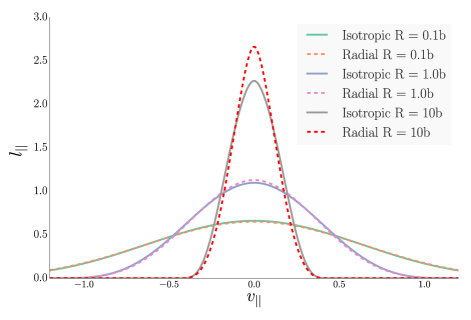
Figure 5: Line–profiles for the two elliptical galaxy models considered. Full lines correspond to the isotropic model and dashed lines are the radially biased model. For each model, the line–profile is plotted at $R=0.1b$, $R=b$ and $R=10b$. We can see that the profiles are indistinguishable at small radii where the models are essentially identical, but then the radially biased model has a narrower line–profile at large radii. We have set $G=M=b=1$ for these models.

6 Dwarf Galaxy DF

Here, we describe another useful DF that can be used to describe the stellar component of dwarf galaxies or globular clusters, and is designed to generate a model close to the Plummer (1911) sphere. We first derive the DF, and then provide an application in which we relax the dwarf galaxy DF within one of our dark matter (Hernquist–like) models.

6.1 Derivation

The Plummer (1911) sphere has gravitational potential and density profiles

$$\Phi(r)=\dfrac{-GM}{\sqrt{r^{2}+b^{2}}}\quad;\quad\rho(r)=\left(\dfrac{3M}{4\mathrm{\pi}b^{3}}\right)\left[1+\left(\frac{r}{b}\right)^{2}\right]^{-5/2}.$$ (43)

The density profile is flat in the centre, then declines as $r^{-5}$ at large radii. Naively, then, one might think that the DF of Equation (16) could be used because the density has two power–law regimes. However, the Plummer sphere is a polytrope with a very simple ergodic DF

$$f(E)\propto E^{7/2},$$ (44)

and so the logic of Section 2.2 no longer applies. As a result, we choose to use a method closer to that employed by Evans & Williams (2014), and construct an approximate Hamiltonian for the Plummer sphere. Consider the Hamiltonian of an isochrone model with mass $M$ and scale–length $b$:

$$H_{\mathrm{iso}}({\boldsymbol{J}})=\dfrac{-(GM)^{2}}{2\left[J_{r}+\frac{1}{2}\left(L+\sqrt{L^{2}+4GMb}\right)\right]^{2}}.$$ (45)

This Hamiltonian varies from the harmonic oscillator when $|{\boldsymbol{J}}|\ll\sqrt{GMb}$ to Keplerian for $|{\boldsymbol{J}}|\gg\sqrt{GMb}$. The Plummer potential of Equation (43) shares the same functional limits with the isochrone. For this reason, we choose to use $H_{\mathrm{iso}}$ as a template for an approximate Plummer Hamiltonian. The selected ansatz is

$$\mathcal{H}({\boldsymbol{J}})=\dfrac{-(GM)^{2}}{\left[g(J_{r})J_{r}+\frac{1}{2}\left(L+\sqrt{\delta^{2}L^{2}+4GMb}\right)\right]^{2}},$$ (46)

where the function $g(J_{r})$ is necessary because the coefficient of $J_{r}$ changes between the two limiting cases, which is not the case for the isochrone. We can analytically solve for the constant $\delta$ and easily select a simple function $g(J_{r})$ to ensure that this Hamiltonian coincides with the correct limits at small and large action. We find;

$$\delta = 4\sqrt{2}-2,$$

$$g(J_{r}) = \dfrac{\sqrt{2}J_{r}+\sqrt{GMb}}{J_{r}+\sqrt{GMb}}.$$ (47)

Now that an approximate Hamiltonian has been constructed, we can substitute into the ergodic DF of the Plummer sphere to find the approximation

$$f({\boldsymbol{J}})=\dfrac{3\mathcal{N}2^{7/2}G^{2}M^{3}b^{2}}{7\pi^{3}}\left[\frac{1}{2}\left(L+\sqrt{\delta^{2}L^{2}+4GMb}\right)+g(J_{r})J_{r}\right]^{-7}.$$ (48)

Figure 6 demonstrates the effectiveness of this DF. The density and circular–speed profiles of the model are in good agreement with the true Plummer model. The model becomes moderately radially anisotropic, where $\beta\simeq 0.2$ at $r\sim 3b$.

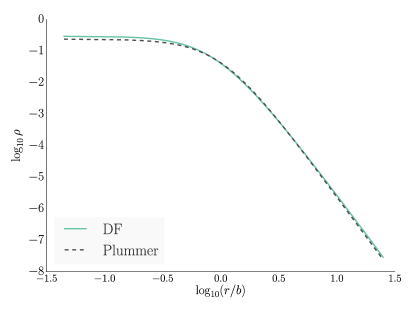
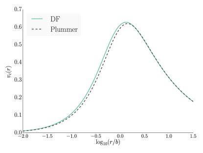
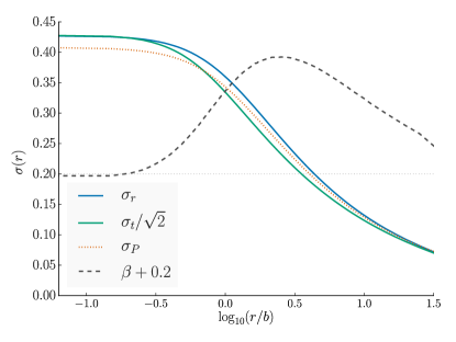
Figure 6: Top row: Comparison of the density profile (left) and circular speed generated (right) by the DF of Equation (48) and the true Plummer model. Bottom: kinematics of the model, we see that the anisotropy parameter peaks at $\sim 0.2$ when $r\sim 3b$. The dotted line depicts the velocity dispersion profile of an isotropic Plummer model ($\sigma_{P}$). We set $G=M=b=1$ for these models.

6.2 Building a Dwarf Galaxy

We now briefly demonstrate the usefulness of $f({\boldsymbol{J}})$ models by relaxing a dwarf galaxy DF and a dark matter DF simultaneously, so that the full DF is given by

$$f({\boldsymbol{J}})=f_{\mathrm{dm}}({\boldsymbol{J}})+f_{*}({\boldsymbol{J}}).$$ (49)

$f_{*}$ is given by the DF of Equation (48) and we choose $f_{\mathrm{dm}}$ to be the cored double power–law with $\alpha=0$ and $\gamma=4$ from Section 4.1.2. We choose the parameters of our dwarf–galaxy to be

$$M_{\mathrm{dm}}=10^{9}{\mathrm{M_{\odot}}}\,,M_{*}=10^{7}{\mathrm{M_{\odot}}}\,,a_{\mathrm{dm}}=1{\mathrm{kpc}}\,,a_{*}=300{\mathrm{pc}}.$$ (50)

where $M_{\mathrm{dm}}$ and $M_{*}$ are the dark matter and stellar masses respectively, whilst $a_{\mathrm{dm}}$ and $a_{*}$ are the scalelengths. This leads to two natural action scales in the model, which are $J_{\mathrm{dm}}=\sqrt{GM_{\mathrm{dm}}a_{\mathrm{dm}}}$ and $J_{*}=\sqrt{GM_{*}a_{*}}$. After constructing the total DF of the model, we used the iterative procedure from Section 2.1 to compute the self–consistant gravitational potential produced by this model. After this calculation is complete, one can compute properties of either component of the model by simply performing integrals over that part of the DF alone. For example, the density of the stellar component of our model is simply given by

$$\rho_{*}(r)=\int{\mathrm{d}}^{3}\boldsymbol{v}\,f_{*}({\boldsymbol{J}}).$$ (51)

In dwarf galaxies, the line–of–sight velocity dispersion, $\sigma_{||}(R)$, of the stars is one of the only kinematic quantities available via observations. To compute this in our model, we evaluate the integral

$$\sigma_{||}^{2}(R)=\dfrac{1}{I_{*}(R)}\int{\mathrm{d}}z\int{\mathrm{d}}v_{x}\int{\mathrm{d}}v_{y}\int{\mathrm{d}}v_{||}\quad v_{||}^{2}f_{*}({\boldsymbol{J}}),$$ (52)

where again $R$ is the projected radius, $z$ is the line–of–sight distance and $v_{x}$, $v_{y}$ are the tangential components of velocity. As in Equation (41), we integrate over bound orbits. Figure 7 depicts this quantity for the model we produce here. We see that the dark matter has produced a largely flat profile as is seen in observations (see e.g., Walker et al., 2009), although as $R\rightarrow 0$ the dispersion increases somewhat. This effect is due to the comparatively modest central mass-to-light ratio in the model, so this is a reasonable representation of a large dwarf spheroidal like Fornax rather than its smaller, overwhelmingly dark matter dominated cousins. We plan to return to the problem of dwarf galaxy modelling in action-angle coordinates in the near future, but this is a simple example of what can be done with these models.

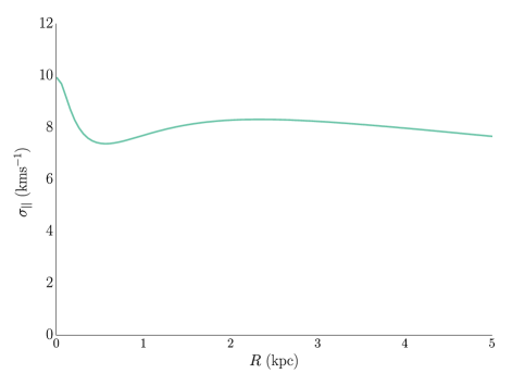
Figure 7: The line–of–sight velocity dispersion profile of the stellar matter in our dwarf galaxy model within $5{\mathrm{kpc}}$. The profile is essentially flat, as is typical in observations of dwarf spheroidals, though there is a slight upturn in the profile as $R\rightarrow 0$.

7 Conclusions

Dynamical models constructed in action coordinates have many desirable properties but, until recently, two issues have stood in the way of their use. First, it was not known how to compute actions in aspherical potentials in the general case. This in turn meant that most astrophysical systems, such as disks or flattened dark matter haloes, could not be modelled. However, the past couple of years have seen rapid development in this area. Binney (2012a) provided an approximate method for computing actions in axisymmetric potentials (refined in Binney 2014) by locally approximating the potential as a Stäckel potential, which was recently generalised to triaxial potentials by Sanders & Binney (2015). An alternative method based on deforming orbital tori by the use of generating functions was also recently discovered by Sanders & Binney (2014) and Bovy (2014), allowing very accurate computation of the actions in wide classes of triaxial potentials.

The second problem was a lack of insight into the form of $f({\boldsymbol{J}})$ for different types of galaxies. The isochrone potential is the only known model with a completely tractable $f({\boldsymbol{J}})$ (e.g., Evans et al., 1990), and techniques had not been developed to construct models suitable for more realistic components of galaxies. Recently, however, Binney (2010, 2012) provided distribution functions for galactic disks, and Pontzen & Governato (2013) suggested an ansatz for a dark–matter halo distribution function. Nonetheless, few models existed with which to construct realistic pressure-supported galaxies. It is this problem that we have addressed in this work. Williams et al. (2014) provided a method for approximating the Hamiltonians of power–law potentials, which can be used to construct Hamiltonians for scaled spherical potentials (Evans & Williams, 2014). In this paper, we have demonstrated how these approximations can be used to construct physically realistic distribution functions for spherical galaxy components. The DFs presented here can also be relatively easily generalised to become flattened, triaxial or rotating by using methods such as action scaling (Binney, 2014). It would seem that now is an exciting time for this field and these models should prove invaluable for understanding our galaxy (e.g. Piffl et al. 2014) and external systems.

We provided two DFs: one designed to emulate double power–law profiles and the other to approximate the Plummer sphere. The double power–law DF has the additional property that one may tune the anisotropy profile by adjusting three of the parameters in the model independently. As such, the DF of Equation (16) can provide a wide variety of models with differing density profiles and kinematics. We then applied this DF in two ways. First, we constructed a model designed to mimic the Hernquist profile and demonstrated that anisotropy tuning is effective at creating a nearly isotropic model, if desired. The model was then altered to become isotropic in the central regions, changing to radial anisotropy at large radii – consistent with the dark matter haloes found in cosmological simulations. This procedure was carried out for both cored and cusped dark haloes. Second, we created a Jaffe–like model to represent an elliptical galaxy. Once again, anisotropy tuning was very effective in creating a very nearly isotropic model. Subsequently, we again changed the kinematics of the model so that it became mildly radially anisotropic in the far–field. As an example of how these models might be applied to data, we computed and compared the line–profiles of the two elliptical galaxy models. Our final section described the derivation of a DF for the stellar component of dwarf galaxies or globular clusters. This DF is derived by explicitly approximating the Hamiltonian of the model, another promising method for constructing $f({\boldsymbol{J}})$ models.

A difficulty with our ansatz for the double power–law DF is that it struggles to replicate models with shallow cusps ($\alpha\sim 0.5$). Experimentation shows that the cusp produced is generally too steep. Although these models are less often used to represent galaxies and dark haloes, it is nonetheless a defect that our ansatz cannot reproduce the full physical range of behaviour. Apparently, the shallow cusped double power–law models do not possess ergodic DFs that are well–represented by double power–laws in binding energy. Interestingly, however, our DF does reproduce cored profiles well. For example, one simply sets $\lambda=0$ to create a model with an isothermal core.

During the completion of this work, Posti et al. (2014) produced a DF closely related to that of Equation (16). Their models, however, differ from ours in several ways. They do not use the Williams, Evans & Bowden (2014) approximation to the Hamiltonian of power-law potentials in the construction of their DF, but instead approximate the equivalent factor to $D_{0}$ by $2$, corresponding to the harmonic oscillator potential. Related to this is that their DF does not contain an equivalent function to $D({\boldsymbol{J}})$, which means that they cannot tune the anisotropy of the models they produce. Finally, they also do not include the variable normalisation factor $T({\boldsymbol{J}})$ in their DF. Nonetheless, the basic approach of the two papers is similar, matching results in different power-law regimes to build double power–law models.

There are a few different directions in which this work could be profitably developed. First, these DFs can be flattened, set rotating or even made triaxial using the previously mentioned approaches already in the literature. It will be interesting to investigate the properties of such models, since they are arguably the simplest avenue available to us for creating self–consistent models of this kind. Another possibility to be explored is the construction of DFs that can well–represent more complex models that are commonly used, such as the Einasto profile. Anisotropy tuning is also a promising technique, as one can conceive of many DFs of the form $f\left[L+D({\boldsymbol{J}})J_{r}\right]$, and perhaps a more flexible, general form for $D({\boldsymbol{J}})$ can be found.

Appendix A Calculating $S_{\alpha}$ and $S_{\gamma}$ when $\gamma=4$

Here, we give an example of the calculation of the relative normalisation factors in the double power–law DF. When $\gamma=4$, these models are known as the Gamma models (Dehnen, 1993; Tremaine et al., 1994). The gravitational potential for such a model ($\gamma\neq 2$) is given by

$$\Phi(r)=-\dfrac{GM}{(2-\alpha)b}\left[1-\left(\dfrac{r}{r+b}\right)^{2-\alpha}\right]$$ (53)

Following Dehnen (1993), we define the following quantities

$$\Psi = -\dfrac{b\Phi}{GM},$$

$$\varepsilon = \dfrac{bE}{GM},$$ (54)

$$y = \left[1-(2-\alpha)\Psi\right]^{1/(2-\alpha)},$$

which means the integral expression for the ergodic DF is

$$f(\varepsilon)=C\int_{0}^{\varepsilon}{\mathrm{d}}\Psi\dfrac{(1-y)^{2}[\alpha+2y+(4-\alpha)y^{2}]}{y^{4-\alpha}\sqrt{\varepsilon-\Psi}},$$ (55)

where $C$ is a constant. We now wish to expand this expression in the limits $\varepsilon\rightarrow 0$ (low binding energies) and $\varepsilon\rightarrow\Psi(0)$ (high binding energies). We restrict ourselves to the cases $0<\alpha<2$. At low binding energies $y\simeq 1-\Psi$ and we can expand the integrand to first order as

$$f(\varepsilon\rightarrow 0)=C\int_{0}^{\varepsilon}{\mathrm{d}}\Psi\dfrac{6\Psi^{2}}{\sqrt{\varepsilon-\Psi}}$$ (56)

giving the result

$$f(\varepsilon\rightarrow 0)=C\dfrac{32}{5}\varepsilon^{5/2}.$$ (57)

In this regime, the binding energy is given by the Kepler Hamiltonian of Equation (14). Upon substitution this gives

$$f(\varepsilon\rightarrow 0) = C\dfrac{32}{2^{5/2}5}(L+J_{r})^{-5}$$

$$\implies S_{\gamma} = \dfrac{32C}{2^{5/2}5}.$$ (58)

We now turn to high binding energies to compute $S_{\alpha}$. Let $\Delta=\Psi(0)-\varepsilon$ and $\Psi(0)-\Psi=x$, so that Equation (55) is written

$$f(\varepsilon)=C\int{\mathrm{d}}x\dfrac{(1-y)^{2}[\alpha+2y+(4-\alpha)y^{2}]}{y^{4-\alpha}\sqrt{x-\Delta}}.$$ (59)

At high binding energies, the integrand is strongly peaked around $x=\Delta$. In this region:

$$y\rightarrow\left[(2-\alpha)x\right]^{1/(2-\alpha)}\rightarrow 0,$$ (60)

Which allows us to expand the integrand, to first order, as

$$f(\varepsilon\rightarrow\Psi(0))=\dfrac{C\alpha}{(2-\alpha)^{(4-\alpha)/(2-\alpha)}}\int_{\Delta}^{\Psi(0)}\dfrac{{\mathrm{d}}x}{x^{(4-\alpha)/(2-\alpha)}\sqrt{x-\Delta}}.$$ (61)

We then Taylor expand the integral in $\Delta$ to give (de Vega & Sanchez, 2014)

$$f(\varepsilon\rightarrow\Psi(0))=C\dfrac{\sqrt{\mathrm{\pi}}\Gamma\left(\frac{1}{2}-\frac{2}{\alpha-2}\right)}{\Gamma\left(\frac{\alpha-4}{\alpha-2}\right)}\dfrac{\alpha}{(2-\alpha)^{(4-\alpha)/(2-\alpha)}}\Delta^{(\alpha-6)/2(\alpha-2)}.$$ (62)

To obtain the DF as a function of the actions, we use the WEB approximation for the Hamiltonian. Using the same definitions for $\epsilon$ and $\zeta$ as in Section 2.2 and setting $v_{0}^{2}=GM/b$, this is given by

$$\mathcal{H}({\boldsymbol{J}})=\dfrac{v_{0}^{2\zeta/\epsilon}}{\zeta b^{\zeta}}(L+DJ_{r})^{\zeta}.$$ (63)

Upon substitution, this finally gives

$$S_{\alpha}=C\dfrac{\sqrt{\mathrm{\pi}}\Gamma\left(\frac{1}{2}-\frac{2}{\alpha-2}\right)\zeta^{(6-\alpha)/2(2-\alpha)}}{\Gamma\left(\frac{\alpha-4}{\alpha-2}\right)}\dfrac{\alpha}{(2-\alpha)^{(4-\alpha)/(2-\alpha)}}.$$ (64)

In practice, we are interested only in the ratio $S_{\alpha}/S_{\gamma}$, because the normalisation factor $\mathcal{N}$ in Equation (16) takes care of absolute differences. To that end, we set

$$S_{\alpha} \rightarrow S_{\alpha}/S_{\gamma},$$

$$S_{\gamma} \rightarrow 1.$$ (65)

A similar calculation for the case $\alpha=0$ leads to $S_{\alpha}=5/4$.

References

- Agnello & Evans (2012) Agnello A., Evans N. W., 2012, ApJL, 754, L39
- Amorisco & Evans (2011) Amorisco N. C., Evans N. W., 2011, MNRAS, 411, 2118
- Amorisco & Evans (2012) Amorisco N. C., Evans N. W., 2012, MNRAS, 419, 184
- Binney (1982) Binney J., 1982, MNRAS, 200, 951
- Binney (2010) Binney J., 2010, MNRAS, 401, 2318
- Binney (2012a) Binney J., 2012a, MNRAS, 426, 1324
- Binney (2012b) Binney J., 2012b, MNRAS, 426, 1328
- Binney (2014) Binney J., 2014, MNRAS, 440, 787
- Binney & Tremaine (2008) Binney J., Tremaine S., 2008, Galactic Dynamics: Second Edition. Princeton University Press
- Bovy (2014) Bovy J., 2014, ApJ, 795, 95
- Breddels & Helmi (2013) Breddels M. A., Helmi A., 2013, AA, 558, A35
- Cappellari et al. (2007) Cappellari M., Emsellem E., Bacon R., Bureau M., Davies R. L., de Zeeuw P. T., Falcón-Barroso J., Krajnović D., Kuntschner H., McDermid R. M., Peletier R. F., Sarzi M., van den Bosch R. C. E., van de Ven G., 2007, MNRAS, 379, 418
- de Lorenzi et al. (2008) de Lorenzi F., Gerhard O., Saglia R. P., Sambhus N., Debattista V. P., Pannella M., Méndez R. H., 2008, MNRAS, 385, 1729
- de Vega & Sanchez (2014) de Vega H. J., Sanchez N. G., 2014, ArXiv e-prints
- Deason et al. (2011) Deason A. J., Belokurov V., Evans N. W., 2011, MNRAS, 411, 1480
- Deason et al. (2011) Deason A. J., McCarthy I. G., Font A. S., Evans N. W., Frenk C. S., Belokurov V., Libeskind N. I., Crain R. A., Theuns T., 2011, MNRAS, 415, 2607
- Dehnen (1993) Dehnen W., 1993, MNRAS, 265, 250
- Dejonghe (1986) Dejonghe H., 1986, Phys. Rep., 133, 217
- Eddington (1915) Eddington A. S., 1915, MNRAS, 76, 37
- Evans (1994) Evans N. W., 1994, MNRAS, 267, 333
- Evans & An (2006) Evans N. W., An J. H., 2006, Phys Rev D, 73, 023524
- Evans et al. (1990) Evans N. W., de Zeeuw P. T., Lynden-Bell D., 1990, MNRAS, 244, 111
- Evans & Williams (2014) Evans N. W., Williams A. A., 2014, MNRAS, 443, 791
- Fillmore (1986) Fillmore J. A., 1986, AJ, 91, 1096
- Goldstein (1980) Goldstein H., 1980, Classical Mechanics: Second Edition. Addison-Wesley
- Governato et al. (2010) Governato F., Brook C., Mayer L., Brooks A., Rhee G., Wadsley J., Jonsson P., Willman B., Stinson G., Quinn T., Madau P., 2010, Nature, 463, 203
- Hansen & Moore (2006) Hansen S. H., Moore B., 2006, New. Ast., 11, 333
- Henon (1959) Henon M., 1959, Annales d’Astrophysique, 22, 126
- Hernquist (1990) Hernquist L., 1990, ApJ, 356, 359
- Hunter & Qian (1993) Hunter C., Qian E., 1993, MNRAS, 262, 401
- Jaffe (1983) Jaffe W., 1983, MNRAS, 202, 995
- Jang-Condell & Hernquist (2001) Jang-Condell H., Hernquist L., 2001, ApJ, 548, 68
- Jeans (1919) Jeans J. H., 1919, Problems of cosmogony and stellar dynamics. Cambridge University Press
- Kronawitter et al. (2000) Kronawitter A., Saglia R. P., Gerhard O., Bender R., 2000, A&AS, 144, 53
- Navarro et al. (1996) Navarro J. F., Frenk C. S., White S. D. M., 1996, ApJ, 462, 563
- Perryman et al. (2001) Perryman M. A. C., de Boer K. S., Gilmore G., Høg E., Lattanzi M. G., Lindegren L., Luri X., Mignard F., Pace O., de Zeeuw P. T., 2001, AA, 369, 339
- Piffl et al. (2014) Piffl T., et al., 2014, MNRAS, 445, 3133
- Plummer (1911) Plummer H. C., 1911, MNRAS, 71, 460
- Pontzen & Governato (2012) Pontzen A., Governato F., 2012, MNRAS, 421, 3464
- Pontzen & Governato (2013) Pontzen A., Governato F., 2013, MNRAS, 430, 121
- Posti et al. (2014) Posti L., Binney J., Nipoti C., Ciotti L., 2014, ArXiv e-prints
- Press et al. (2007) Press W. H., Teukolsky S. A., Vetterling W. T., Flannery B. P., 2007, Numerical Recipes 3rd Edition: The Art of Scientific Computing, 3 edn. Cambridge University Press, New York, NY, USA
- Richardson & Fairbairn (2014) Richardson T., Fairbairn M., 2014, MNRAS, 441, 1584
- Sanders & Binney (2014) Sanders J. L., Binney J., 2014, MNRAS, 441, 3284
- Sanders & Binney (2015) Sanders J. L., Binney J., 2015, ArXiv e-prints
- Schwarzschild (1979) Schwarzschild M., 1979, ApJ, 232, 236
- Shu (1967) Shu F. H., 1967, ApJ, 158, 505
- Strigari et al. (2014) Strigari L. E., Frenk C. S., White S. D. M., 2014, ArXiv e-prints
- Syer & Tremaine (1996) Syer D., Tremaine S., 1996, MNRAS, 282, 223
- Teyssier et al. (2011) Teyssier R., Moore B., Martizzi D., Dubois Y., Mayer L., 2011, MNRAS, 414, 195
- Tremaine et al. (1994) Tremaine S., Richstone D. O., Byun Y.-I., Dressler A., Faber S. M., Grillmair C., Kormendy J., Lauer T. R., 1994, AJ, 107, 634
- Walker et al. (2009) Walker M. G., Mateo M., Olszewski E. W., Peñarrubia J., Wyn Evans N., Gilmore G., 2009, ApJ, 704, 1274
- Walker & Peñarrubia (2011) Walker M. G., Peñarrubia J., 2011, ApJ, 742, 20
- Wilkinson & Evans (1999) Wilkinson M. I., Evans N. W., 1999, MNRAS, 310, 645
- Williams et al. (2014) Williams A. A., Evans N. W., Bowden A. D., 2014, MNRAS, 442, 1405
- Wojtak et al. (2013) Wojtak R., Gottlöber S., Klypin A., 2013, MNRAS, 434, 1576
- Wojtak & Łokas (2010) Wojtak R., Łokas E. L., 2010, MNRAS, 408, 2442
- Wojtak & Mamon (2013) Wojtak R., Mamon G. A., 2013, MNRAS, 428, 2407