Precise Radial Velocities of Giant Stars

Abstract

Context. We have obtained precise radial velocities for a sample of 373 G and K type giants at Lick Observatory regularly over more than 12 years. Planets have been identified around 15 of these giant stars, and an additional 20 giant stars host planet candidates.

Aims. We are interested in the occurrence rate of substellar companions around giant stars as a function of stellar mass and metallicity. We probe the stellar mass range from approximately 1 to beyond 3 M_⊙, which is not being explored by main-sequence samples.

Methods. We fit the giant planet occurrence rate as a function of stellar mass and metallicity with a Gaussian and an exponential distribution, respectively.

Results. We find strong evidence for a planet-metallicity correlation among the secure planet hosts of our giant star sample, in agreement with the one for main-sequence stars. However, the planet-metallicity correlation is absent for our sample of planet candidates, raising the suspicion that a good fraction of them might indeed not be planets despite clear periodicities in the radial velocities. Consistent with the results obtained by Johnson for subgiants, the giant planet occurrence rate increases in the stellar mass interval from 1 to 1.9 M_⊙. However, there is a maximum at a stellar mass of $1.9^{+0.1}_{-0.5}$ M_⊙, and the occurrence rate drops rapidly for masses larger than 2.5–3.0 M_⊙. We do not find any planets around stars more massive than 2.7 M_⊙, although there are 113 stars with masses between 2.7 and 5 M_⊙ in our sample (corresponding to a giant planet occurrence rate smaller than 1.6% at 68.3% confidence in that stellar mass bin). We also show that this result is not a selection effect related to the planet detectability being a function of the stellar mass.

Conclusions. We conclude that giant planet formation or inward migration is suppressed around higher mass stars, possibly because of faster disk depletion coupled with a longer migration timescale.

1 Introduction

About 1500 confirmed extrasolar planets are known today (Wright et al. 2011). The rate of detection and confirmation of exoplanets has increased dramatically in the recent past, with almost one third of exoplanets confirmed in early 2014 alone (Rowe et al. 2014; Lissauer et al. 2014) and another third being discovered only during the last two years. Roughly two thirds of all confirmed planets have been found with the transiting method, and many more candidates are known, especially those discovered with the Kepler space telescope (see Borucki et al. 2011a, b; Batalha et al. 2013 for Kepler planet candidates and Howard et al. 2012; Fressin et al. 2013 for statistical analyses of planet occurrence rates). The radial velocity (RV) technique, which accounts for the detection of the remaining third of confirmed planets, has major difficulties with the detection of planets around stars more massive than $\approx 1.5\,\mathrm{M_{\sun}}$, since hotter stars have fewer absorption lines and also rotate more rapidly, which both adversely affect the radial velocity precision (Galland et al. 2005a; Lagrange et al. 2009). A few giant planets and brown dwarfs have been found around early dwarf stars despite these difficulties (see e.g. Galland et al. 2005b, 2006).

In order to avoid these difficulties one can target moderately massive stars that have already left the main sequence and have evolved into giant stars. As giant stars are cooler than their predecessors on the main sequence and have slower rotation rates, their spectral lines are more numerous and also less broadened, so that one can measure their radial velocities very precisely.

While the statistics on properties of extrasolar planets around main-sequence stars has continuously improved throughout the last decade, the number of known substellar companions around giant stars is still comparatively small. So far, 63 companions in 59 systems have been announced. They have emerged from a variety of Doppler surveys, including our own using the Hamilton Spectrograph at Lick Observatory (Frink et al. 2001, 2002; Reffert et al. 2006; Mitchell et al. 2013; Trifonov et al. 2014) as well as surveys conducted with FEROS at La Silla Observatory (Setiawan et al. 2003, 2005), with the HIDES spectrograph at Okayama Observatory (Sato et al. 2003, 2007, 2008a, 2008b, 2010, 2012), Tautenburg (Hatzes et al. 2005; Döllinger et al. 2007, 2009b, 2009a), the Penn State Torún planet search with the Hobby-Eberly Telescope (Niedzielski et al. 2007, 2009a, 2009b; Gettel et al. 2012a, b), the BOES spectrograph at Bohyunsan Observatory (Han et al. 2010; Lee et al. 2012a, b, 2013), and the search by Jones et al. (2011, 2013, 2014a, 2014b), which employs FEROS at La Silla Observatory as well as the FECH and CHIRON spectrographs at Cerro Tololo Inter-American Observatory.

The planet-metallicity correlation (Fischer & Valenti 2005; Udry & Santos 2007) is by now well established for main-sequence stars, indicating that a star with high metallicity has a much higher probability of hosting a planet than a star with a lower metallicity. For subgiants, the same trend with metallicity was observed by Johnson et al. (2010a), although it is not as strong as for main-sequence stars. In addition to metallicity, Johnson et al. (2010a) also found a correlation between planet occurrence rate and stellar mass in the sense that higher mass stars have a higher probability of hosting a giant planet. In the case of planet-hosting evolved stars it is not clear yet whether a correlation between planet occurrence rate and metallicity exists. While Pasquini et al. (2007), Takeda et al. (2008) and Mortier et al. (2013) do not find evidence for such a correlation in their samples of G and K giants, Hekker & Meléndez (2007) find indications for a positive correlation between metallicity and planet occurrence rate for K giant stars. However, one has to keep in mind that the number of securely established planets around evolved stars originating from a single homogeneously selected and observed sample was still quite small at that time.

Recently, Maldonado et al. (2013) have reinvestigated a possible link between metallicity and giant planet occurrence rate in a sample of published subgiant and giant planet hosts, using a control sample of nearby Hipparcos giants (which were not actually searched for planets and which is certainly not ideal - given the huge number of bright giant stars slightly different selection criteria can result in a sample with different characteristics). Maldonado et al. (2013) found no planet-metallicity correlation for giant stars with stellar masses smaller than 1.5 M_⊙, but did find a positive planet-metallicity correlation for giant stars with masses larger than 1.5 M_⊙ and for subgiants. The issue of a planet-metallicity correlation for giant stars is thus far from settled.

In this paper we search for correlations between planet occurrence rate and either stellar metallicity and/or stellar mass in our sample of 373 G and K giants, which we have been monitoring at Lick Observatory since 1999. In particular, stellar masses in our parent sample range from about 1 to 5 M_⊙ and thus extend significantly beyond the mass range of the combined main-sequence and subgiant sample from Johnson et al. (2010a), which covers the mass range from 0.2 to 2 M_⊙. Our detection capability of planetary companions is similar to that used in other studies: for about 60% of our monitored stars, we are sensitive to planets with an RV semi-amplitude of 30 m/s and a period less than 4 years, which corresponds to the detection threshold used by Fischer & Valenti (2005).

According to the usual definition involving deuterium burning, one would have to call objects with masses of more than about 13 M${}_{\mbox{\tiny Jup}}$ (Spiegel et al. 2011) brown dwarfs rather than planets. However, taking also the formation scenario into account, one might want to include objects in the mass range from roughly 13 to 25–30 M${}_{\mbox{\tiny Jup}}$ among the planet category, especially those which formed around stars more massive than 1 M_⊙ (see e.g. Baraffe et al. 2010; Schneider et al. 2011). We will not make a distinction at the deuterium burning mass, but rather call all these objects planets (or planet candidates) for simplicity.

The paper is organized as follows. In Section 2 we describe the Doppler survey at Lick Observatory. Section 3 is dedicated to the characterization of the stellar sample and in particular describes how we derive stellar masses for our sample of giant stars. The planets that we have found in our sample are discussed in Section 4. In Section 5 we statistically analyze planet occurrence rate as function of stellar metallicity and stellar mass and present our results. Section 6 provides a detailed discussion of our results including a comparison with planet formation models, and finally we give a short summary in Section 7.

2 Observations

Since 1999, we have been carrying out a radial velocity survey of G and K giants at UCO/Lick Observatory using the 0.6 m Coudé Auxiliary Telescope (CAT) together with the Hamilton Echelle Spectrograph with a theoretical resolution of approximately 60 000 (Vogt 1987); in practice we measure a resolution of about 50 000 at a wavelength of 6000 Å. See Frink et al. (2001, 2002); Reffert et al. (2006) for a description of our survey and earlier results. We follow the method for acquiring and reducing data using the iodine cell method as described by Butler et al. (1996) and achieve a typical RV precision of about 5–8 m s^-1 with integration times of less than 30 minutes. We typically have accumulated between 20 and 100 observations per star, depending on brightness and observing priority.

Giant stars exhibit solar-like oscillations (see e.g. Zechmeister et al. 2008), which manifest themselves as RV jitter in our observations due to the low observing cadence. The amount of RV jitter depends on spectral type (Frink et al. 2001; Hekker et al. 2006), with typical values of below 10–20 m s^-1 for early K giants and up to 50 m s^-1 or more for late K giants and early M giants. Thus, an RV precision of 5–8 m s^-1 is adequate for our survey.

3 Stellar Sample

3.1 Sample Selection Criteria

The selection criteria for the stars have been described by Frink et al. (2001). The stars are all brighter than 6${}^{\mbox{\tiny th}}$ mag in $V$ and have declinations between $-30^{\circ}$ and $+68^{\circ}$. The original sample only consisted of 86 K giants that were supposedly neither variable nor part of a multiple system; we especially checked a number of flags in the Hipparcos Catalogue in order to make sure that there are no indications for so far unresolved companions (see appendix in Frink et al. 2001). Another 96 stars were included one year later with basically the same selection criteria; the only difference was that for the newly added stars photometric stability was not required anymore (the coarse variability flag in the Hipparcos Catalogue was allowed to be non-zero). However, it turned out that the actual level of photometric variability is not very different between the two parts of the sample; photometric variability is usually smaller than 0.01 mag and basically insignificant, so that we treat these two parts of the sample together. Three of the stars were excluded from the sample when they were found to be visual binaries.

In 2004 the survey was extended again by 194 G and K giants that have, on average, higher masses and bluer color $(0.8\leq B-V\leq 1.2)$. Bluer color means less intrinsic RV jitter (Frink et al. 2001; Hekker et al. 2006), which was the reason for the inclusion of late G giants. The selection of stars was performed in the following way. In a first step, we identified all the G and K giant stars in the Hipparcos Catalogue with relevant position, apparent magnitude and color (see above) via their reduced proper motion diagram, which nicely separates giant and dwarf stars based on their distinct kinematics. For this sample, we estimated masses from evolutionary tracks (Girardi et al. 2000) assuming solar metallicity. In the end, we chose those stars with the highest masses derived in this way. Binaries were also avoided as much as possible, but some have slipped in nevertheless.

The reason for preferentially selecting more massive stars was to test whether or not more massive stars also host more massive companions. In retrospect we realized that these selection criteria for this sample were not ideal for the issues addressed in this paper. As we did not have metallicities on hand for these stars, the stellar masses were initially derived assuming solar metallicity. However, the derivation of the masses used in this paper does take metallicity into account, as described below.

3.2 Stellar Masses

The stellar masses have been determined using a trilinear interpolation between evolutionary tracks and isochrones (Girardi et al. 2000), respectively, and metallicity as a third parameter (Künstler 2008). Because the location of evolutionary tracks and isochrones depends on the assumed metallicity, taking into account the metallicities is crucial. Most of the metallicities were derived from the equivalent widths of iron lines by Hekker & Meléndez (2007). We performed the interpolation for separate stages of the evolutionary tracks and isochrones in order to determine the probabilities for the stars to be on the red giant branch (RGB) or on the horizontal branch (HB), respectively. For each star we generated 10 000 positions within the three-dimensional space $(B-V,\,M_{\mathrm{V}},\,\left[\mathrm{Fe/H}\right])$, using the measured color, absolute magnitude and metallicity and taking Gaussian errors into account. For each of these generated positions we determined the stellar parameters from evolutionary tracks by interpolation. The results have been weighted by the initial mass function (IMF),

$$\mathrm{d}N\propto M^{-\alpha}\mathrm{d}M\quad,$$ (1)

where we adopted a value of $\alpha=2.35$ from Salpeter (1955). In addition to the IMF, the evolutionary timescale at a given position in the color-magnitude diagram (CMD),

$$v=\frac{\sqrt{\left(\Delta\left(B-V\right)\right)^{2}+\left(\Delta M_{\mathrm{V}}\right)^{2}}}{\Delta t}$$ (2)

has been taken into account for the weighting. $v$ is the velocity in the CMD, at the position indicated by the star’s $B-V$, $M_{V}$ and [Fe/H] values, or at the generated Monte Carlo position in the CMD which is consistent with the observational errors in those quantities. This means that the probability for a star to be located at a certain position in the CMD is lower the faster its evolution progresses at that particular position in the CMD. Taken together, the weighting with the IMF and the evolutionary timescale during the red giant phase closely resembles weighting with a present-day mass function for giant stars. Counting the successful interpolations and weighting the results in the above-mentioned way yields the probabilities and masses of a star being either on the RGB or on the HB. The masses assuming either RGB or HB evolutionary status are mostly very similar to each other, with significant differences only in a few cases. We provide our derived masses with errors and probabilities for both evolutionary cases in Table LABEL:allstars. In this paper we simply use the mass which has the higher probability.

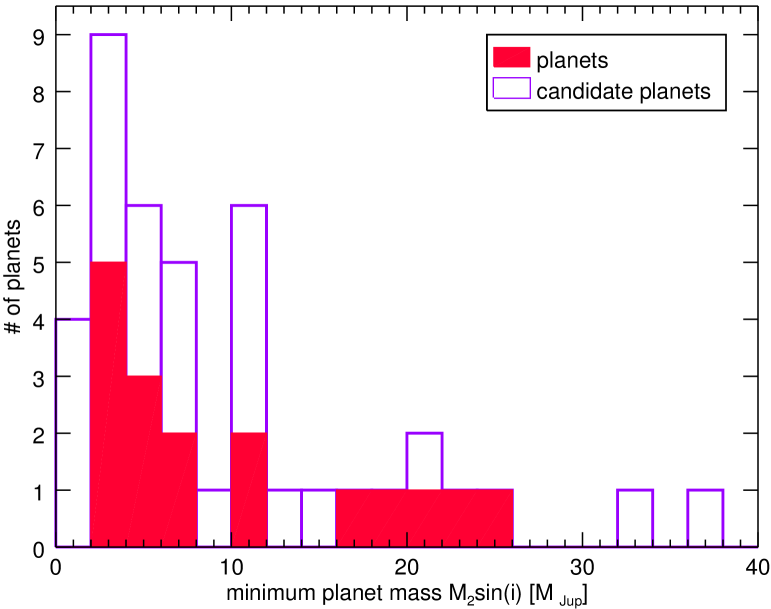
Figure 1: Histogram of minimum masses derived for 17 secure and 26 planet candidates in our Lick sample. Two of the 26 planet candidates have minimum masses larger than 40 M${}_{\mbox{\tiny Jup}}$ and are not shown in the plot.

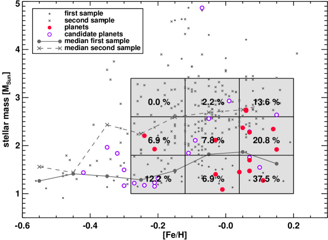
Figure 2: Planet occurrence rate as a function of metallicity and stellar mass in our Lick sample. The percentage numbers give the fraction of the number of stars with a planet and/or planet candidate of all stars in that bin. One can clearly see that planet occurrence rate in our Lick sample increases strongly with stellar metallicity and decreases with stellar mass.

Recently, Lloyd (2011, 2013) and Schlaufman & Winn (2013) have argued that masses derived from evolutionary models for subgiant and giant stars are systematically too large. The argument from Lloyd (2011, 2013) rests on the comparison of the mass distribution of planet host subgiants with a mass distribution constructed by integrating stellar model isochrones, taking the IMF, metallicity distribution and star formation history into account. Schlaufman & Winn (2013) argue that the distribution of galactic space motions of subgiant and giant planet hosts shows that the population has been dynamically heated and is thus of lower mass than assumed so far. Johnson et al. (2013) point out that the discrepancy in the mass distributions of subgiant planet hosts and model mass distributions based on galactic population synthesis may be the result of selection effects in the planet host sample, and conclude that the masses derived on the basis of evolutionary tracks might still be correct.

Similarly, there are many selection effects biasing the masses in our K giant sample, and one should not expect that the masses follow those in an unbiased galactic model. Specifically, our Lick sample consists of three subsamples with different selection criteria. The sample is neither magnitude- nor volume-limited, but has been selected to contain the most photometrically and astrometrically stable stars available, based on a number of flags in the Hipparcos Catalogue. Specifically, one of the subsamples was selected to contain the highest mass G and K giants, in order to better test planet occurrence rate as a function of mass. Thus, the statistical tests of Lloyd (2011, 2013) and Schlaufman & Winn (2013) do not necessarily apply to our sample.

We simply note that while it is possible that our masses suffer from systematic errors in the underlying evolutionary tracks, the masses for our Lick sample would all be affected in the same way, provided that the systematic error shifts a particular evolutionary track in the CMD, but does not significantly affect its shape. This implies that a comparison of the properties of the higher mass stars of the sample to those of the lower mass stars in the sample is still possible and not affected by an incorrect mass scale.

An independent test would be to determine asteroseismic masses for some of the evolved stars in order to test spectroscopically determined masses; for some stars in our Lick sample, the Kepler K2 mission will provide the necessary data. Johnson et al. (2014) compare mass determinations for the subgiant HD 185351, and find general agreement between the asteroseismic and spectroscopic mass at  1.8 M_⊙; only once asteroseismology is combined with interferometry, the resulting mass estimate would be smaller by 2.6 $\sigma$. Asteroseismic masses are available for two stars in our Lick sample: the planet-bearing stars $\iota$ Dra (Baines et al. 2011) and $\beta$ Gem (Hatzes et al. 2012). In both cases, the asteroseismic masses are compatible with the spectroscopic masses at a level of about 1-1.5 $\sigma$; for $\iota$ Dra the asteroseismic mass is the larger one, for $\beta$ Gem the spectroscopic one. A much larger sample would be needed to unveil any systematic differences between the various methods to derive stellar masses.

3.3 Stellar Parameter Table

Besides stellar mass, the interpolation also yields other stellar parameters, namely integrated mass loss $M_{\mathrm{loss}}$ (as compared to the zero age main-sequence masses), age $t_{*}$, effective temperature $T_{\mathrm{eff}}$, luminosity $L$, radius $R_{*}$ (computed from the two previous quantities) and surface gravity $\log g$. Table LABEL:allstars provides these stellar parameters along with their formal errors as well as the $\left[\mathrm{Fe/H}\right]$ values for each star.

4 Substellar Companion Statistics

Our goal is to investigate giant planet occurrence as a function of stellar mass and metallicity. In order to do so, we need to identify all potential planets that have emerged from our Lick RV survey of G and K giant stars.

Since giant stars show larger RV jitter than main-sequence stars, it is sometimes difficult to distinguish between an RV signal caused by a companion and RV variations with an intrinsic stellar origin. In particular, non-radial pulsations could have similar periods as the planets we typically observe in our sample. Non-radial pulsations have been identified in giant stars on the basis of both Corot and Kepler data (see e.g. De Ridder et al. 2009; Carrier et al. 2010; Bedding et al. 2010; Stello et al. 2013), but it is not clear at present whether such single-mode, long-lived non-radial pulsations with high radial order (Hatzes & Cochran 1999) as would be required to match the observed radial velocities really exist in giant stars.

Radial pulsations are not a concern since they have much shorter timescales, confirmed recently for red giants in large numbers via asteroseismology performed with Kepler data, such as in Bedding et al. (2010), Kallinger et al. (2012), or Stello et al. (2013); they manifest themselves as stellar jitter in our RV curves.

Likewise, stellar spots which could in principle give rise to radial velocity variations with the stellar rotation period can be excluded as the major contribution to the observed radial velocity variability, since the spots would have to be too large to be consistent with the low level of photometric variability observed by Hipparcos. This was shown explicitly to be the case for the planets orbiting the K giants $\tau$ Gem and 91 Aqr in Mitchell et al. (2013) and for the interacting planets around the K giant $\eta$ Cet (Trifonov et al. 2014), and also applies to all other planets and planet candidates in the Lick sample; none of the observed radial velocity variations is consistent with being caused by a spotted star, in particular due to the very low level of photometric variability.

We verified this again for all the planets and planet candidates discussed here, applying two tests. For the first test, we derived the spot filling factor which would be required to generate the observed RV amplitude using the relation from Hatzes (2002), estimated the resulting photometric variability by factoring in the geometry and compared this to the photometric variability observed by Hipparcos. In many cases, in particular for those companions with short periods and consequently large RV amplitudes, this resulted in spot filling factors larger than 5–10%, which cannot be brought in line with the small photometric variations observed by Hipparcos. For the second test, we assumed that the RV periods which we observe match the rotation period, and calculated the resulting rotational velocity $v_{\mathrm{rot}}$ utilizing the derived stellar radii from Table LABEL:allstars. We compared this to the measured projected rotational velocities $v\cdot\sin i$ from Hekker & Meléndez (2007). In most cases the rotational velocities $v_{\mathrm{rot}}$ are significantly smaller than the projected rotational velocities, which is not possible. This applies specifically to the stars with longer periods and thus smaller rotational velocities $v_{\mathrm{rot}}$, increasing the discrepancy. In other words, the periods which we see in the RV data are typically larger than the rotational periods of the stars. These tests clearly showed that rotational modulation of stellar features is not a viable explanation for the observed RV variability.

The typical level of intrinsic radial velocity variation scales with $B-V$ (Frink et al. 2001) and/or surface gravity (Hekker et al. 2008); while the expected stellar jitter of our late G and early K giants is less than approximately 20 m s^-1, the jitter for late K giants (with $B-V$ around 1.6) is up to 100 m s^-1 and more. As a result, smaller mass or longer period planets, which have smaller RV semi-amplitudes, cannot be identified as easily as those around main-sequence stars. One needs more observations to compensate for the stellar jitter, and longer time baselines covering several periods to ensure that phase and amplitude of the observed RV signal are constant over time.

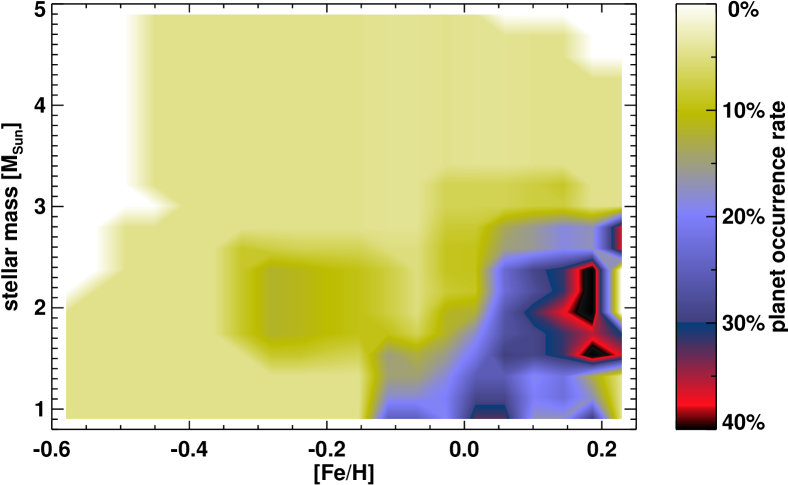
Figure 3: Planet occurrence rate (color coded) as a function of metallicity and stellar mass in our Lick sample; only the secure planets have been considered. Data have been heavily smoothed, so that the general trend in planet occurrence rate becomes apparent. There is a clear maximum in planet occurrence rate for metallicities of about 0.2 and masses of about 2 M_⊙.

For these reasons we have divided the tentative detections present in our Lick sample into two categories: planets and planet candidates. Planets are those which we consider secure discoveries, and planet candidates are those whose existence is more doubtful. Planets usually have a clear and convincing periodic RV signal, and have been observed over several cycles. Planet candidates also have clear periodic signals (highly significant in Lomb-Scargle periodograms), but the ratio between RV semi-amplitude and stellar jitter is smaller than for the secure planets, so that stellar jitter becomes more prominent in the RV curve.

Distinguishing planet candidates from non-radial pulsations is rather difficult and requires many observations over a long time baseline in order to test for phase and amplitude stability of the RV signal. Another possibility to distinguish between pulsations and an orbiting companion is the comparison of the RV signal computed from different wavelength regions of the spectrum. We have started observing 20 K giants with periodic radial velocity patterns from our Lick sample with the CRIRES infrared high resolution spectrograph at VLT. These observations should ultimately tell us whether the periodic RV pattern is due to a companion (same pattern in the Lick and CRIRES velocities) or not (different amplitude and/or phase in Lick and CRIRES velocities), after we have accumulated observations over several years.

In our Lick sample, we have identified secure planets around 15 stars. Two of these have an additional secure planet and two an additional planet candidate. We found planet candidates around 20 stars; four of these have an additional planet candidate. Two stars display a linear trend in the radial velocities on top of the planet candidate periodicity, which could be indicative of substellar objects in very long orbits, but are not considered here further. Two secure planets and four planet candidates are found in spectroscopic binaries. Altogether, this adds up to 43 (candidate) planets in 35 systems.

A histogram of minimum planet masses is shown in Fig. 1. The smallest minimum mass of a secure planet is 2.3 M${}_{\mbox{\tiny Jup}}$, while the smallest minimum mass of a planet candidate is 1.1 M${}_{\mbox{\tiny Jup}}$. On the other hand, the largest minimum mass among secure planets is 25 M${}_{\mbox{\tiny Jup}}$, while a few planet candidates could have masses even more massive than that (but still rather uncertain because of long period orbits which still need to close). As mentioned earlier, we refer to all of these objects as planets (or planet candidates).

Eight of the 15 systems with a secure planet in our Lick sample have been published already: $ι$ Dra~b (Frink et al. 2002), Pollux~b (Reffert et al. 2006; Hatzes et al. 2006), $ε$ Tau~b (Sato et al. 2007), 11~Com~b (Liu et al. 2008), $ν$~Oph~b and c (Quirrenbach et al. 2011; Sato et al. 2013), $τ$~Gem~b and 91~Aqr~b (Mitchell et al. 2013), and $η$~Cet b and c (Trifonov et al. 2014); we will publish the remaining ones in the near future.

5 Planet Occurrence Rate as a Function of Stellar Mass and Metallicity

5.1 Whole Sample

In Fig. 2, we plot stellar mass as a function of metallicity for all our stars in the Lick sample. We distinguish the 186 stars with which we started in 1999/2000 (dots; ‘first sample’) from the 196 ones which were added in 2004 with different selection criteria (crosses; ‘second sample’). The solid and dashed lines indicate the median masses per metallicity bin of the stars of the first and second sample, respectively. One can clearly see that the stars of the second sample have higher masses than the stars of the first sample, in particular at high metallicities. It was our aim to study exoplanets around high mass stars when we put together the second sample, so this bias was introduced on purpose through our selection criteria.

Table 1: Number of stars with planets ($n_{\mbox{\tiny planet}}$), with planet candidates ($n_{\mbox{\tiny cand}}$) and number of all stars ($n_{\mbox{\tiny stars}}$) in our Lick sample for the bins in metallicity ([Fe/H]${}_{\mbox{\tiny bin}}$) and stellar mass ($M_{\mbox{\tiny*,bin}}$) shown in Fig. 2. The corresponding planet frequencies for planets ($f_{\mbox{\tiny planet}}$) and for planets and planet candidates combined ($f_{\mbox{\tiny planet+cand}}$) are also given, together with their 68.3% confidence levels derived from binomial statistics.

[Fe/H]${}_{\mbox{\tiny bin}}$	$M_{\mbox{\tiny*,bin}}$	$n_{\mbox{\tiny planet}}$	$n_{\mbox{\tiny cand}}$	$n_{\mbox{\tiny stars}}$	$f_{\mbox{\tiny planet}}$	$f_{\mbox{\tiny planet+cand}}$
[dex]	[M⊙]				[%]	[%]
–0.28 … –0.12	1.0 … 1.8	0	5	41	00.0 ${}^{+4.3}_{-0.0}$	12.2 ${}^{+7.0}_{-3.4}$
	1.8 … 2.6	2	0	29	06.9 ${}^{+7.9}_{-2.3}$	06.9 ${}^{+7.9}_{-2.3}$
	2.6 … 3.4	0	0	21	00.0 ${}^{+8.0}_{-0.0}$	00.0 ${}^{+8.0}_{-0.0}$
–0.12 … +0.04	1.0 … 1.8	2	0	29	06.9 ${}^{+7.9}_{-2.3}$	06.9 ${}^{+7.9}_{-2.3}$
	1.8 … 2.6	1	3	51	02.0 ${}^{+4.2}_{-0.6}$	07.8 ${}^{+5.5}_{-2.3}$
	2.6 … 3.4	0	1	45	00.0 ${}^{+3.9}_{-0.0}$	02.2 ${}^{+4.8}_{-0.7}$
+0.04 … +0.20	1.0 … 1.8	4	2	16	25.0 ${}^{+13.3}_{-7.7}$	37.5 ${}^{+12.9}_{-10.1}$
	1.8 … 2.6	4	1	24	16.7 ${}^{+10.2}_{-5.0}$	20.8 ${}^{+10.4}_{-5.9}$
	2.6 … 3.4	2	1	22	09.1 ${}^{+9.9}_{-3.1}$	13.6 ${}^{+10.5}_{-4.4}$

In order to study planet occurrence rate as a function of metallicity and mass, we divided the area which is most populated in the metallicity/stellar mass plane into nine bins (three in each dimension); see Fig. 2 and Table 1. We then determined the fraction of stars with planets (filled circles) and planet candidates (open circles) in each of these bins. The resulting planet occurrence rates (counting planets as well as planet candidates) are overplotted in Fig. 2 in the center of each bin (percentage numbers).

Table 1 gives the number counts of planets, planet candidates and stars in each bin, and the resulting planet occurrence rates counting only secure planets ($f_{\mbox{\tiny planet}}$) and counting secure planets as well as planet candidates ($f_{\mbox{\tiny planet+cand}}$). 68.3% confidence limits on planet occurrence rates are also given; they were calculated based on binomial statistics following the Bayesian approach (Cameron 2011).

From Fig. 2 and Table 1, a rather clear pattern emerges: planet occurrence rate increases strongly with metallicity in our sample, and it decreases with stellar mass in the mass range which we probe here. Planet occurrence rate is highest (37.5 ${}^{+12.9}_{-10.1}$%) in the bin with the highest metallicities and the lowest stellar masses, and it drops down to 0% in the mass bin with the lowest metallicities and highest stellar masses. In between, we observe intermediate values, so there seems to be a smooth transition between the highest and lowest planet occurrence rates as a function of metallicity and stellar mass.

This result does not change much when we reject the planet candidates and only use the confirmed planets for the statistics, as one can see from a comparison of the last two columns in Table 1. Of course, the overall planet occurrence rate is lower if only confirmed planets are counted. The fraction of stars with confirmed giant planets, $f_{\mbox{\tiny planet}}$, can be regarded as a lower value for the true fraction of giant stars harboring giant planets in our sample, while the fraction of stars which either harbor a confirmed planet or a planet candidate, $f_{\mbox{\tiny planet+cand}}$, can be regarded as an upper value for that number.

The correlations with metallicity and mass which we described above are present irrespective of whether planet candidates are included or excluded. However, if considering the distribution of planets and planet candidates separately, one notable difference emerges: we find a lot of planet candidates at rather small metallicity and mass. In our lowest mass and lowest metallicity bin, we only find planet candidates, but no planets. This trend continues to smaller metallicities. We do not know what the reason is for the different distribution of planets and planet candidates with respect to metallicity, but it is certainly possible that some fraction of the planet candidates are not true planets.

We will now examine the correlation of planet occurrence rate with stellar metallicity and stellar mass in more detail. For this analysis, we restrict ourselves to the planet population of the confirmed planets only. We divided our Lick sample of stars into more metallicity and mass bins (namely, 20 bins over the full range of values shown in Fig. 2), and determined planet occurrence rates in those bins. Since we are plagued by small number statistics with such a large number of bins, we heavily smoothed the resulting planet occurrence rate map using a sliding average over five bins, in order to reveal the general trends present in the distribution of planets, but not the small, insignificant details. The resulting planet occurrence rate map is shown in Fig. 3.

Planet occurrences rate is color coded as indicated by the bar on the right hand side of the plot; the planet occurrence rate ranges from 0% (the large area of the diagram in light yellow, especially at small metallicity and high mass) up to 40% for metallicities around 0.2 and masses around 2 M_⊙ (black). The white areas of the diagram correspond to metallicity/mass combinations for which we do not have any measurements, i.e. which are not covered by our Lick sample.

5.1.1 Fitted Dependencies

In order to quantify the planet occurrence rate as a function of metallicity and stellar mass, and in order to compare our results with the findings of others, we fitted our data to a model following an exponential distribution in metallicity and a Gaussian distribution in stellar mass, as suggested by Fig. 3. In addition, we also fitted our data with a power law distribution in stellar mass (see Johnson et al. 2010a), which we modified also to include an exponential cutoff so that it better describes the decrease in planet occurrence rate at higher masses. For comparison, we also fitted our observations to a flat distribution in mass, keeping only the exponential distribution in metallicity.

The Gaussian plus exponential distribution has the following form with parameters $C$, $\mu$, $\sigma$ and $\beta$:

$$f(M_{*},\mbox{[Fe/H]})=C\,\exp\left({-\frac{1}{2}\left[\frac{M_{*}-\mu}{\sigma}\right]^{2}}\right)\,10^{\beta\mbox{\tiny[Fe/H]}}\qquad,$$ (3)

whereas the power law with cutoff plus exponential distribution is described by

$$f(M_{*},\mbox{[Fe/H]})=C\,(M_{*}/\mbox{M}_{\odot})^{\alpha}\,\exp\left({-\frac{M_{*}}{M_{0}}}\right)\,10^{\beta\mbox{\tiny[Fe/H]}}\qquad,$$ (4)

with parameters $C$, $\alpha$, $M_{0}$ and $\beta$. The power law plus exponential distribution with parameters $C$, $\alpha$ and $\beta$ as used by Johnson et al. (2010a) has the form

$$f(M_{*},\mbox{[Fe/H]})=C\,(M_{*}/\mbox{M}_{\odot})^{\alpha}\,10^{\beta\mbox{\tiny[Fe/H]}}\qquad.$$ (5)

$f(M_{*},\mbox{[Fe/H]})$ is the fraction of stars with giant planets, $M_{*}$ is the stellar mass and [Fe/H] is the stellar metallicity.

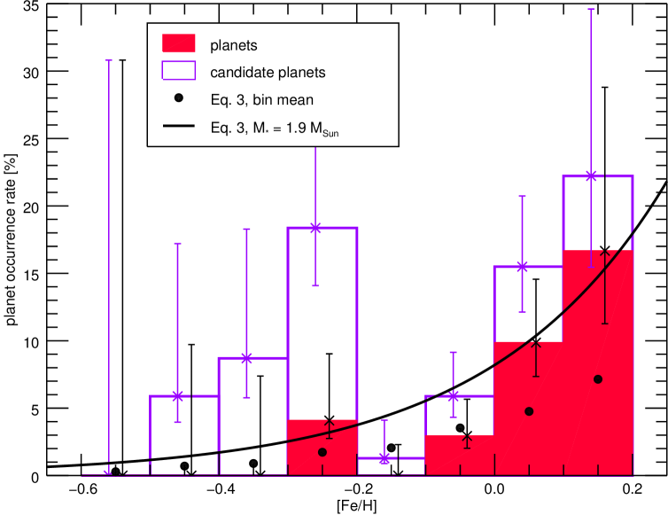
Figure 4: Planet-metallicity correlation observed in our Lick sample, ignoring the effect of stellar mass on the planet occurrence rate. The filled histogram shows secure planets, whereas the open histogram includes planet candidates as well. Error bars are computed based on binomial statistics as explained in the text. The solid line illustrates the exponential fit to the planet occurrence rate of secure planets as a function of metallicity, for a stellar mass of 1.9 M_⊙. The black dots also correspond to the exponential fit, but here the individual mass distribution in each bin has been taken into account.

We performed the fitting with two different methods: Levenberg-Marquardt least squares minimization and Bayesian inference. The results were largely identical, so we quote only the results of the Bayesian analysis in Table 2. The disadvantage of the least squares minimization in our context is its inability to account for asymmetric error bars, as applicable for binomial population proportions. On the other hand, the Bayesian technique has some shortcomings as well; we performed a simple grid search for the maximum likelihood, which is computationally expensive, and the choice of priors or meaningful parameter intervals is rather arbitrary.

An advantage of Bayesian inference for the given analysis is the possibility to account for a probability distribution in mass, rather than assuming one fixed value with an error bar. We constructed these probability distributions by adding two Gaussians (where applicable), which were centered on the two different mass estimates which we derived for most of our stars (Table LABEL:allstars). The formal errors of the masses correspond to the widths of the Gaussians, and the relative heights were given by the probabilities derived for the red giant branch and the horizontal branch solution, respectively. We thus ended up with bimodal distributions for the masses, although in many cases the two peaks in the mass probability distribution are located close to each other.

Our strategy for applying the principles of Bayesian inference closely followed the one outlined in Johnson et al. (2010a). Specifically, we would like to stress that we fitted the various planet occurrence models to each star individually, not to binned or smoothed data. We chose uniform priors for all parameters, since we did not want to bias the result in any way. We ensured that all prior ranges included the peak in the maximum likelihood as well as the 68.3% confidence regions of the parameters.

The result of the Bayesian fitting is summarized in Table 2. The first line gives the limits of the uniform prior ranges. The parameters given for each model correspond to the peak in the likelihood function; the 68.3% confidence intervals are quoted in the second line for each fitted model. Most posterior probability distribution functions are slightly asymmetric; the quoted confidence intervals thus correspond to the shortest intervals with a 68.3% chance for containing the correct parameter values. The Bayes factor $B$ is the ratio of the evidence of a given model divided by our best fitting model described by Eq. 3. Bayes factors between 1 and 3.2 are ‘not worth more than a bare mention’, whereas Bayes factors between 10 and 100 provide ‘strong evidence’ against the model being tested (Kass & Raftery 1995).

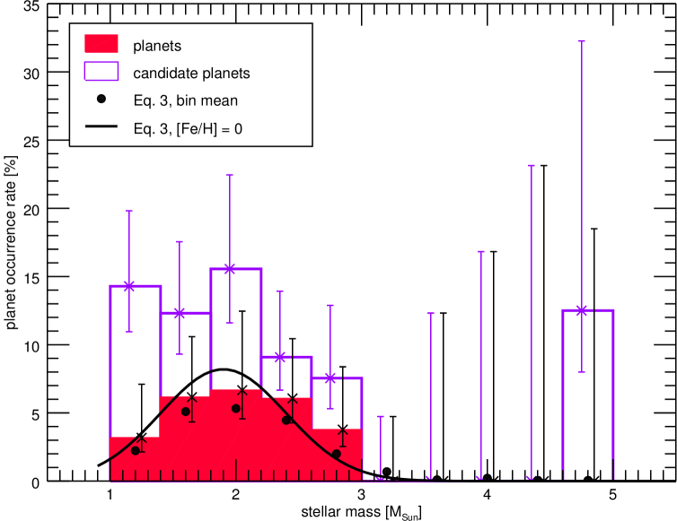
Figure 5: Planet occurrence rate as a function of stellar mass in our Lick sample, ignoring the effect of stellar metallicity. See caption of Fig. 4 for the explanation of histogram data and error bars. The solid line denotes our best fit to the mass dependence of the giant planet occurrence rate computed for zero metallicity. The black dots correspond to the same model, but the true metallicity distribution within each bin has been taken into account.

Table 2: Derived parameters, 68.3% confidence regions and Bayes factors $B$ obtained via Bayesian fitting of observed planet occurrence rates as a function of stellar mass and metallicity; see Eqs. 3, 4 and 5. Parameter values from other studies are given for comparison.

	$\alpha$	$\beta$	$C$	$\mu$	$\sigma$	$M_{0}$	B	mass range
				[M⊙]	[M⊙]	[M⊙]		[M⊙]
new Bayesian fits
uniform prior limits	–1.5…+1.5	0.0…3.0	0.01…0.30	1.0…3.0	0.1…2.0	0.5…2.0
Eq. 3	…	1.7	0.082	1.9	0.5	…	1.0	1.0 …5.0
	…	1.3 - 2.0	0.056 - 0.122	1.4 - 2.0	0.3 - 1.0	…	(fixed)	…
Eq. 4	1.0	1.8	0.223	…	…	0.7	1.3	1.0 …5.0
	(fixed)	1.3 - 2.0	0.111 - 0.432	…	…	0.6 - 1.0	…	…
Eq. 5	–0.3	1.6	0.089	…	…	…	8.4	1.0 …5.0
	–0.6 - 0.0	1.2 - 1.9	0.059 - 0.124	…	…	…	…	…
flat	…	1.8	0.044	…	…	…	76	1.0 …5.0
	…	1.3 - 2.1	0.031 - 0.060	…	…	…	…	…
other investigations
Johnson et al. (2010a)	$1.0\pm 0.3$	$1.2\pm 0.2$	$0.07\pm 0.01$	…	…	…		0.2 …2.0
Udry & Santos (2007)	…	$2.04$	$0.0301$	…	…	…		0.7 …1.4
Fischer & Valenti (2005)	…	$2.0$	$0.03$	…	…	…		0.7 …1.5

The Gaussian distribution in mass (Eq. 3) and the power law with cutoff (Eq. 4) fit the data about equally well. Our best fitting model is the one with the Gaussian distribution in mass; we obtain $C=0.082^{+0.040}_{-0.026}$, $\beta=1.7^{+0.3}_{-0.4}$, $\mu=1.9^{+0.1}_{-0.5}$ M_⊙ and $\sigma=0.5^{+0.5}_{-0.2}$ M_⊙. The parameter $\mu$ gives the stellar mass with the highest probability for the presence of a giant planet. Furthermore, according to this model, the planet occurrence rate has dropped to half of its peak value at masses of 1.2 M_⊙ and 2.6 M_⊙, respectively. The uncertainty in these masses is of the order of 0.5 M_⊙ (combined error in both $\mu$ and $\sigma$).

A flat distribution in mass or the simple power law from Johnson et al. (2010a) perform much worse; the evidence against those latter two models is ‘strong’ (Kass & Raftery 1995), so that they can be rejected. The power law exponent $\alpha$ in the model from Johnson et al. (2010a) is even negative when fitted for with our data, suggesting that the decrease of planet occurrence rate at higher masses dominates over its increase observed for smaller masses. This is why we fixed $\alpha$ to 1, the value obtained by Johnson et al. (2010a), when modeling our observations according to Eq. 4. We also tried to fit for $\alpha$ here, but did not succeed; the parameter is not well constrained by our data, and is correlated with $M_{0}$.

The value that we find for $\beta$ is fully consistent with other studies on the planet-metallicity correlation, in particular with Fischer & Valenti (2005) and Udry & Santos (2007) (Table 2). For the mass range from 0.2–2 M_⊙, Johnson et al. (2010a) found a positive correlation between planet occurrence rate and stellar mass. It seems that this correlation turns into an anticorrelation for masses larger than about 1.9 M_⊙.

In Fig. 4 we show the planet occurrence rate as a function of metallicity, and in Fig. 5 we show the planet occurrence rate as a function of stellar mass, respectively. Separate histograms are plotted for either only the secure planets or including planet candidates. The solid line and the black dots indicate the fit which was obtained above from applying Eq.3 to the individual data (secure planets only), not the histogram data shown in the plots which either ignores the dependence of planet occurrence rate on mass (Fig. 4) or on metallicity (Fig. 5). It consists of an exponential for the dependence on metallicity (Fig. 4) and a Gaussian for the dependence on stellar mass (Fig. 5).

Ignoring the effect of stellar mass (Fig. 4, histogram data), the planet-metallicity correlation seems even steeper than compared to the fit that takes both metallicity and stellar mass into account (Fig. 4, black dots). It is also evident from Fig. 4 that the planet candidates are distributed differently with respect to stellar metallicity than the secure planets; no clear planet-metallicity correlation is seen for the planet candidates alone.

The distribution of secure planets and planet candidates, respectively, with respect to stellar mass (Fig. 5) is rather similar to each other; we do not see any differences in the two distributions such as those observed in the planet-metallicity correlation of the two planet samples.

Fig. 6 shows contours of equal Bayesian likelihood as a function of parameters $\beta$ and $\mu$ of our best-fitting model (Eq. 3). There is no correlation between the two parameters characterizing the dependence of giant planet occurrence rate on stellar mass and metallicity, respectively. This indicates that the giant planet occurrence rate depends on both parameters directly, independently of each other, and is not due e.g. to the uneven distribution of stars in the mass-metallicity plane.

The most striking result of our analysis is clearly the sharp decrease in planet occurrence rate for stars with masses higher than 2.5 to 3 M_⊙. The highest mass of a planet bearing star in our sample is 2.7 M_⊙. We do not find any confirmed planets around stars with larger masses, although there are 119 such stars in our sample (83 of those stars are in the mass range from 2.7 to 3.5 M_⊙). This corresponds to a giant planet occurrence rate of $<1.6$% at 68.3% confidence, and $<5.6$% at 99.73% confidence in the mass interval from 2.7 to 5.0 M_⊙. We will discuss the dependence of giant planet occurrence rate on stellar mass further in Section 6.

5.2 Subsamples

In the previous section we have taken our full sample as a reference, assuming that we would be able to detect giant planets with periods up to a few years around any star in our sample. Here we will show that even when cutting down our sample to ensure uniform detectability of planets, the results of the previous section still hold.

There are three parameters that influence our capability to detect a given planet around a particular star in our sample: stellar mass, intrinsic stellar jitter, and number of observations. Observing time span does not matter in our context, because all stars have been observed for at least six years. With the exception of the period of the outer companion in the resonant double brown dwarf system $\nu$ Oph, the periods for confirmed planets in our sample range from 0.5 to 2.3 years.

The radial velocity semi-amplitude $K_{1}$, which is imposed by a planet with given mass $m_{2}$, period $P$ and eccentricity $e$ on a star of mass $M_{*}$, is given by

$$K_{1}=\left(\frac{2\pi G}{P}\right)^{1/3}\frac{1}{\sqrt{1-e^{2}}}\,\,\frac{m_{2}\sin i}{\left(M_{*}+m_{2}\right)^{2/3}}\qquad,$$ (6)

where $i$ is the inclination and $G$ is the gravitational constant.

We consider a given planet around a given star detectable in our survey if the radial velocity semi-amplitude that it would generate is larger than the intrinsic stellar jitter (any orbital motion is subtracted from the observed velocities before the intrinsic stellar jitter is derived from the standard deviation of the radial velocities). Furthermore, we require at least 12 observations for each star, in order to allow for the detection of the planetary signal in the presence of stellar jitter. The median intrinsic stellar jitter in our sample is 22 m s^-1, while the RV semi-amplitude $K_{1}$ of a planet with a mass of 2.3 M${}_{\mbox{\tiny Jup}}$ (smallest mass among our confirmed planets), period of 2.3 years (largest period among our confirmed planets) around a 2 M_⊙ star (typical stellar mass) is 31 m s^-1.

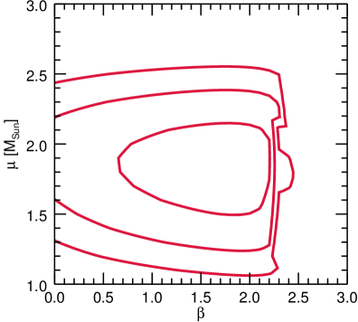
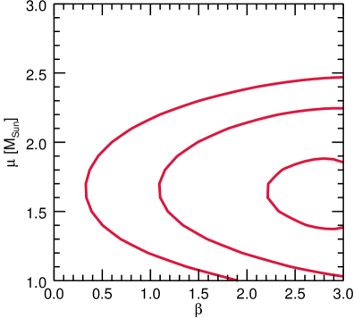
Figure 6: Contours of equal Bayesian likelihood as a function of parameters $\beta$ and $\mu$ for our best-fitting model (Eq. 3). The panel on the left corresponds to the full Lick sample, while the panel on the right corresponds to the subsample. In both cases no correlations between the parameters $\beta$ (related to metallicity) and $\mu$ (related to mass) can be seen, indicating that the giant planet occurrence rate indeed depends on both, stellar mass and metallicity.

For comparison, the detection capability threshold used by Fischer & Valenti (2005) corresponds to an RV amplitude of at least 30 m s^-1, a period of less than 4 years, and at least 10 observations per star, very similar to our requirements. The subgiant planet hosts analyzed statistically by Johnson et al. (2010a) also have Doppler signals which are typically larger than 20–30 m s^-1, so that the detection threshold between the various surveys is not that different; we only miss a few planets with very small RV amplitudes in our Lick giant star survey in comparison with other surveys.

However, we caution that the resulting planets to which we are sensitive will be more massive, for two reasons: (1) Since the radial velocity signal depends on stellar mass (Eq.6), and our stars are more massive than those in typical main-sequence Doppler samples (average mass of about 2 M_⊙ for giant stars as opposed to 1 M_⊙ for main-sequence stars), the resulting planet masses in our sample are larger by a factor of about 1.6. The same is true, though with even smaller differences in resulting planet masses, for subgiants (typical stellar mass 1.5 M_⊙). (2) The distribution of orbital parameters of planets found around giant stars and those found around main-sequence or subgiant stars differ, most notably in period. While a few hot Jupiters are known around subgiant stars (Johnson et al. 2006, 2010b), such short-period planets are completely absent from giant star samples; they are either engulfed by the star or move further out as the radius of the stellar host increases (Sackmann et al. 1993; Villaver & Livio 2009). In fact, roughly half of our stars are on the horizontal branch already (as opposed to the red giant branch), and have thus experienced a short phase with a very expanded shell at the end of the red giant branch, potentially altering the observable planets’ orbital parameters. Larger period however means smaller RV signal, which can only be compensated by a larger planet mass.

Our goal is to assemble a subsample that is more uniform in planet detectability than our full Lick sample, in order to eliminate any potential biases in the planet occurrence rate as a function of metallicity and stellar mass that result from reduced planet detection capabilities around stars of high mass, large jitter or poor observing history. For each star in the full Lick sample, we check whether a planet with a minimum mass of 2.3 M${}_{\mbox{\tiny Jup}}$ (which corresponds to the smallest planet mass among our confirmed planets) and a period of 2.3 years (which corresponds to the longest period among our confirmed planets, with the exception of the outer companion to $\nu$ Oph) would be detectable according to the definition above.

We end up with 207 (out of 373) stars that fulfill the detectability criteria and which thus constitute our subsample. Among the rejected stars are three planet-bearing stars and seven additional stars hosting planet candidates. While we managed to detect a (massive or small period) planet around these stars, it means we would not have been able to detect the small planet which we defined as reference for detectability.

The subsample still contains 50 out of the 119 stars with stellar masses larger than 2.7 M_⊙ from our original sample. Thus, the fraction of high mass stars in the subsample (24%) is a bit smaller than in the full sample (32%), but not by as much as one might expect. The reason is that the more massive stars in our sample have less than average jitter (due to our original selection criteria), which makes up for the reduced planet detection capability around a star of larger mass.

In Fig. 7 we show a comparison of planet occurrence rates in the full sample and the subsample for the same bins as in Table 1. One can clearly see that the planet occurrence rates in the various stellar mass and metallicity bins are very similar between the full and the restricted samples. The small differences are not significant if the errors are taken into account. Errors vary greatly across bins, but are typically of the order of 5-10% for the full sample (see Table 1), and not very different for the subsample (typically of the order of 1% larger).

Furthermore, one can clearly discern the two bins where planet-bearing stars were rejected for the subsample; these are those where the planet occurrence rate drops. The only two planet-bearing stars in the lowest metallicity and medium mass bin were removed, as well as one planet-bearing star in the highest metallicity highest mass bin. For the remaining bins, planet occurrence rates either remain at zero or increase slightly, reflecting the removal of a few stars without planets in those bins.

The overall pattern in the dependence of planet occurrence rate with mass and metallicity which we observed for the full sample is still clearly visible for the subsample and does not appear to have changed significantly. We fitted the planet occurrence rate for the subsample as a function of stellar mass and metallicity to the same models as for the full sample. Unfortunately, the Bayesian fitting did not work as well for the subsample as for the full sample, presumably because increasingly large parts of the mass-metallicity plane are not sampled well, and the overall number of stars is small. This means that we cannot assign reliable confidence limits to the derived parameters; we still managed to derive best-fit values for all parameters from a clear maximum in the likelihood function. Least-squares minimization worked well though, and was consistent with the results from Bayesian fitting. Yet, for consistency with the last section, we quote the results from Bayesian fitting for the subsample as well.

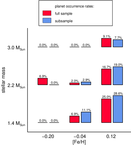
Figure 7: Comparison of the planet occurrence rates for our full sample and the subsample which ensures uniform detection capability (ensuring detectability of a planet of at least 2.3 M${}_{\mbox{\tiny Jup}}$ with a period up to 2.3 years). The planet occurrence rates in both sample are very similar in the various stellar mass and metallicity bins; the small differences are not significant.

Just as for the full sample, the model consisting of an exponential distribution in metallicity and a Gaussian distribution in mass (Eq. 3) performed best. We obtained the following parameters: $C=0.079$, $\beta=2.8$, $\mu=1.6$ M_⊙, and $\sigma=0.6$ M_⊙. These parameters are very similar to those derived for the full sample, with the exception of the parameter $\beta$, which indicates a steeper planet-metallicity correlation than for the full sample. However, considering that the errors for the subsample are certainly somewhat larger than for the full sample, the results are fully consistent with each other, and the differences are not significant.

The fitting of a four parameter model to the subsample data is clearly stretching the statistical analysis to the limits; after all, the subsample data just consist of 12 planets around 207 stars, distributed over mass and metallicity space. Clearly, a much larger sample with uniform detection capability with respect to planets would be desirable, but will not be available in the near future. Nevertheless, the subsample data clearly support our most important finding, namely that the giant planet occurrence rate decreases sharply for stellar masses larger than 2.5–3.0 M_⊙. In the subsample, we still have 50 stars with masses larger than 2.7 M_⊙, around which no planet has been found. This corresponds to a giant planet occurrence rate smaller than 3.5% at 68.3% confidence, significantly different from the giant planet occurrence rates for lower mass and higher metallicity bins.

From the comparison of results for the full sample and the subsample we conclude that no obvious biases are present in the analysis of our full sample. We confirm a strong planet-metallicity correlation based on our subsample analysis, and a peak in planet occurrence rate for stellar masses somewhere in the interval between 1.5 and 2 M_⊙, with a strong decline in giant planet occurrence rate for stars with masses larger than 3 M_⊙.

6 Discussion

6.1 Correlation of Giant Planet Occurrence Rate with Stellar Metallicity

We find a strong planet-metallicity correlation in our Lick sample of G and K giants, with about the same power law exponent (to within the errors) as observed for main-sequence stars by Fischer & Valenti (2005) and Udry & Santos (2007); see Table 2). Johnson et al. (2010a) also observed a positive planet-metallicity correlation in a sample of subgiant stars, yet with a smaller power law exponent (possibly because of the simultaneous fitting for the correlation with stellar mass and the distribution of stars in the mass-metallicity plane).

The parameter $\beta$ which describes the planet-metallicity relation is remarkably constant across models, irrespective of the model used to describe the mass dependence of the giant planet occurrence rate. This indicates already that we are really dealing with two separate effects here, and planet occurrence rate does indeed depend on both, stellar mass and stellar metallicity.

However, our finding is in sharp contrast to the results of Pasquini et al. (2007) and Takeda et al. (2008), who did not find the same correlation of planet occurrence rate with metallicity as the one observed for main-sequence stars in their giant star samples. One reason could be that their selection criteria for confirmed planets were not as strict as ours. In fact, our planet candidates do not show a strong planet-metallicity correlation; many planet candidates are found around lower-metallicity stars. It is indeed notoriously difficult to distinguish giant stars harboring true planets from giant stars which show (multi-)periodic radial velocity variations not due to planets (see Section 4). We only used secure planets when deriving our planet-metallicity correlation, which is essential. Since the secure planet and the planet candidate samples show a different distribution with respect to metallicity, we believe that our sample of planet candidates is a true mixture of stars with true planets and stars without any planets.

In fact, this same argument can also explain the results from Maldonado et al. (2013), who noted a difference in planet occurrence rate and metallicity between low-mass and high-mass giant stars. If we divide our sample of secure planet and planet candidate hosts at a stellar mass of 1.5 M_⊙ just as they did, we also do not observe a strong planet-metallicity correlation for the lower mass sample, but a strong planet-metallicity correlation for the higher mass sample (see Fig 2). The reason for this is that the planet candidates are preferentially found at lower metallicity and also at lower mass and thus pollute the strong planet-metallicity correlation of the secure planets. The different findings for lower and higher mass giant stars could thus simply be a consequence of a polluted sample of planet hosts with non-planet bearing stars.

We conclude that there are strong indications for a planet-metallicity correlation among giant star planet hosts which matches the observed planet-metallicity correlation for main-sequence planet hosts.

6.2 Anticorrelation of Giant Planet Occurrence Rate with Stellar Mass

The most striking result of our analysis of giant planet occurrence rate as a function of stellar metallicity and stellar mass is clearly the steep decline of planet occurrence rate for masses larger than 2.5 to 3 M_⊙. Indeed we do not find any confirmed planet around a star with a mass higher than 2.7 M_⊙, although there are 113 such stars in the sample. Thus, the planet occurrence rate for stars with masses in the range 2.7–5 M_⊙ is consistent with zero ($0.0^{+1.6}_{-0.0}$%).

Our Lick K giant survey is the first Doppler survey that covers the mass range between 2 and 5 M_⊙; traditional Doppler surveys have looked primarily at late-type main-sequences stars with typical masses between 0.7 and at most 1.5 M_⊙ (Fischer & Valenti 2005; Udry & Santos 2007). A notable exception is the Doppler survey of subgiants by Johnson (Johnson et al. 2010a), which covers stellar masses up to about 2 M_⊙. Interestingly, Johnson et al. (2010a) found that the planet occurrence rate increases with mass up to masses of about 2 M_⊙.

This is also the case in the Lick K giant survey: stars with masses of about 2 M_⊙ have the highest planet occurrence rates observed, significantly higher than those for stars of about 1 M_⊙. However, this trend reverses for even higher stellar masses, beyond about 2.5–3 M_⊙.

Burkert & Ida (2007) have identified a lack of massive planets at intermediate orbital distances for main-sequence stars in the mass range from 1.2–1.5 M_⊙ as compared to planets found around stars with a mass range from about 0.7–1.2 M_⊙. These differences in planet properties occur at smaller masses than relevant here, yet this might be a first indication that higher stellar masses adversely affect planet formation. Burkert & Ida (2007) attributed the observed differences in planet properties to a shorter disk depletion timescale for more massive stars, which could be caused by either a smaller disk size or stronger extreme ultraviolet flux as compared to those around lower mass stars.

Ida & Lin (2005) and Kennedy & Kenyon (2008b) both considered giant planet formation around stars of various masses using a semi-analytic formation model. The details of the models differ significantly, yet both predict an increase in the giant planet formation rate with mass over the range from about 0.5 to 1.5 M_⊙ (Ida & Lin 2005) and from about 0.5 to 3.0 M_⊙ (Kennedy & Kenyon 2008b), respectively (see Fig. 7 of Kennedy & Kenyon 2008b). After a sharp maximum, the giant planet formation rate strongly decreases with stellar mass in both models. Qualitatively, this is exactly what we observe, at a mass which falls exactly in the mass range predicted by those two models.

The increase in planet occurrence rate with stellar mass can be interpreted as being the result of the larger disk masses of more massive stars. Neptune mass planets are frequent around lower mass stars according to those models, consistent with observations, but giant planets form only rarely around lower-mass stars (Johnson et al. 2007). Higher disk masses increase the chance of forming a planet in general and a giant planet in particular, and thus the overall planet occurrence rate correlates with stellar mass.

The reason why this positive correlation between planet occurrence rate and stellar mass breaks down at masses larger than about 2.5–3 M_⊙ can be understood as follows. As the mass of the star increases, the snow line, at or beyond which most planets are thought to form, is located increasingly further out ($a_{\mbox{\tiny snow}}\propto M_{*}^{\alpha}$, with $\alpha$ between 1 and 2 (Ida & Lin 2008; Kennedy & Kenyon 2008a). At increasing distances from the star, gas densities and Kepler velocities are smaller, which both slows down growth rates. As a result, the migration time scale $\tau_{\mbox{\tiny mig}}$ is also longer ($\tau_{\mbox{\tiny mig}}\propto M_{*}^{1.5}$, Kennedy & Kenyon 2008a), while stellar disk dispersal is faster (Kennedy & Kenyon 2009). Thus, the slower growth rate, increased migration time scale and short lifetime of the protostellar disk might prevent stars with masses larger than $2.5-3$ M_⊙ from forming giant planets that would be observable at semi-major axes of a few AU today, as probed by our survey.

6.3 Effect of Stellar Evolution?

Little is known about the fate of planets as the host star evolves from the main sequence up the giant branch. Some calculations have been carried out specifically for the solar system, with specific consideration of the question whether or not the Earth will eventually be engulfed by the Sun during its post-main sequence evolution.

In the model by Sackmann et al. (1993) the Earth can evade being swallowed, whereas the model by Schröder & Connon Smith (2008) predicts that the Earth will be engulfed by the Sun before it reaches the tip of the red giant branch. All studies agree, however, on an increase of Earth’s orbital distance during the early post-main sequence evolution of the Sun, which is due to conservation of angular momentum as the Sun loses mass; mass loss dominates over tidal interactions between the Earth and the Sun as well as over dynamical drag, which both tend to shrink Earth’s orbit. The disagreement on the final fate of the Earth mainly comes from different assumptions about mass loss, to which the models are rather sensitive.

Sato et al. (2008a) have discussed possible planet engulfment during post-main sequence evolution in order to explain the observed lack of close-in planets for intermediate mass stars, while Villaver & Livio (2009) and Kunitomo et al. (2011) have derived the orbital evolution of planets during the post-main sequence evolution of stars more massive than the Sun. Their model calculations included changes in the orbital distance of a planet induced by stellar mass loss and stellar tides, through conservation of angular momentum; an essential part of the model calculations are stellar evolutionary models. Villaver & Livio (2009) also included frictional and gravitational drag forces, but since their effect was found to be negligible those effects were not included by Kunitomo et al. (2011). The result of the model calculations are the time-dependent orbital distances of planets during the stars’ red giant branch and horizontal branch phases of stellar evolution, from which the minimum orbital distance of a planet required to avoid engulfment by the star (critical initial semi-major axis or survival limit) can be derived.

In summary, the orbital distances of the inner planets become smaller (eventually leading to engulfment), while the orbital distances of the outer planets become larger during the red giant and horizontal branch stages of the parent star. The largest changes in the orbital distances occur at the tip of the red giant branch, when the stellar radius is largest and tidal effects become much more important. The critical initial semi-major axis of a planet to avoid engulfment by the parent star is strongly dependent on stellar mass, and to a lesser extent on planet mass and stellar metallicity, with a sharp transition at stellar masses of around 2 M_⊙ which is due to the presence of the helium flash leading to an increase in stellar radius for stars with masses smaller than about 2 M_⊙ and the absence of such an effect for stars with masses larger than about 2 M_⊙ (Kunitomo et al. 2011). The detailed predictions for the critical semi-major axis for survival are quite different between the models from Villaver & Livio (2009) and Kunitomo et al. (2011), presumably due to differences in their assumptions about stellar evolution.

These studies illustrate that the properties of any planetary system will be subject to profound changes during the post-main sequence evolution of its host star. It is thus possible that the properties of the planet population which we observe in our Lick giant star sample are not the same as they were while the host stars were still on the main sequence. Depending on the age of the stars, significant orbital evolution could already have taken place. Age determination of the giant stars is rather difficult, but we estimated the probabilities for each star to either be on the red giant branch or on the horizontal branch, respectively (given in Table LABEL:allstars in the appendix). We find that the parent stars of 12 out of 15 confirmed planets (80%) are more likely on the horizontal branch than on the red giant branch; for the planet candidates, only 8 out of 20 parent stars (40%) are on the horizontal branch. For comparison, 41% of the stars in the whole Lick sample are on the horizontal branch, 56% are on the red giant branch; for the remaining 3% we could not determine an evolutionary state. Thus the fraction of stars with confirmed planets that are already on the horizontal branch is relatively large, and some orbital evolution could certainly have taken place already.

Villaver & Livio (2009) and Kunitomo et al. (2011) compare their critical survival orbital distances with the orbital distances of planets detected around stars more massive than 1.5 M_⊙, and find that all observed planets orbit at orbital distances large enough to avoid engulfment during the red giant and horizontal branch stellar evolutionary phases, and especially the phase at the tip of the red giant branch when the stellar radius is largest. Our confirmed planets have orbital distances larger than the survival limit for the models of Kunitomo et al. (2011) only, while it looks as if some of their orbits could be in conflict with the predictions by Villaver & Livio (2009). However, for a definitive conclusion one would have to compute specific limits for every system separately, taking its orbital characteristics and masses into account.

Most importantly, Kunitomo et al. (2011) find that for stars more massive than about 2.5 M_⊙, there is a large gap between the critical orbital distance and the orbital distance distribution found among observed planets. Thus, it looks as if another mechanism besides engulfment plays a major role in shaping the observed semi-major axis distribution of giant planets around intermediate mass stars, preventing orbits too close in. Kunitomo et al. (2011) conclude that most likely giant planet formation is hindered for stars more massive than about 2.5 M_⊙.

Due to the large gap between the predictions for the survival limit and the observed distribution of orbital distances, planet engulfment does not play a major role for the interpretation of the observed planet occurrence rate as a function of mass for the Lick sample. It is very well possible that some planets around stars in our sample might have been engulfed already, but this could not explain why we do not find any giant planets around stars more massive than 2.5–3.0 M_⊙, in particular since the survival line is much closer in for stars more massive than about 2 M_⊙ than for less massive stars. Most likely, giant planets around stars more massive than 2.5–3 M_⊙ are not being formed at separations of a few AU in the first place, rather than being engulfed or kicked out during stellar evolution later on.

7 Summary

We have analyzed the distribution of planet-bearing stars in our Lick sample of 373 G and K giants with respect to metallicity and stellar mass. Altogether, we find secure planets around 15 stars and planet candidates around 20 stars, from a Doppler survey running over twelve years. We are sensitive towards giant planets; minimum planet masses for the secure planets range from 2.3 to 25 M${}_{\mbox{\tiny Jup}}$. We obtain the following results:

1. We find a strong planet-metallicity correlation for the secure planets in our Lick sample, with a power law exponent of $1.7^{+0.3}_{-0.4}$ that matches the planet-metallicity correlations derived for main-sequence stars (Fischer & Valenti 2005; Udry & Santos 2007).

2. Giant planet occurrence rate and stellar mass are strongly correlated. Based on a Gaussian fit the planet occurrence rate is highest for a stellar mass of $1.9^{+0.1}_{-0.5}$ M_⊙, and decreases rapidly for stars with masses larger than 2.5–3.0 M_⊙. The width $\sigma$ of the Gaussian distribution is $0.5^{+0.5}_{-0.2}$ M_⊙. The giant planet occurrence rate in the stellar mass interval from 2.7 to 5.0 M_⊙ is $<1.6$% with 68.3% confidence.

3. We repeat the statistical analysis on a subsample of our full Lick sample which ensures uniform planet detection capability (in terms of number of observations, stellar jitter and stellar mass). Since we obtain the same results for the subsample as for the full sample to within the statistical errors, we conclude that our analysis of the full sample is not severely biased.

4. We do not find a planet-metallicity correlation for the planet candidates in our sample. We conclude that at least some of the planet candidates may not be real, despite clear periodicities in their radial velocities.

5. A strong decrease in planet occurrence rates for stellar masses above roughly 1.5 to 3 M_⊙ is predicted in the semi-analytic planet formations models by Ida & Lin (2005) and Kennedy & Kenyon (2008a). The decrease in giant planet occurrence rates might be explained by a smaller growth rate, longer migration timescale and the shorter lifetime of the protostellar disk for the more massive stars compared to the less massive ones.

6. The observed paucity of giant planets for stars more massive than 2.5–3 M_⊙ is most likely not due to stellar evolutionary effects which might influence the orbital parameters of orbiting planets. More likely, giant planets with periods up to several years are not being formed in the first place.

Table 3: Stellar mass $M_{*}$, metallicity $[\mathrm{Fe/H}]$, effective temperature $T_{\mathrm{eff}}$, luminosity $L$, surface gravity $\log g$, radius $R_{*}$, integrated mass loss $M_{\mathrm{loss}}$ and age $t_{*}$ for all 373 giant stars of the Lick sample. The last column indicates whether the parameters refer to the star being on the red giant branch (RGB) or horizontal branch (HB), respectively, while the second but last column gives the corresponding probability $P$. The $\dagger$ symbol marks the stars for which our interpolation did not yield any results.

Identifier	$M_{*}$	$\sigma_{M_{*}}$	$[\mathrm{Fe/H}]$	$\sigma_{[\mathrm{Fe/H}]}$	$T_{\mathrm{eff}}$	$\sigma_{T_{\mathrm{eff}}}$	$L$	$\sigma_{L}$	$\log g$	$\sigma_{\log g}$	$R_{*}$	$\sigma_{R_{*}}$	$M_{\mathrm{loss}}$	$\sigma_{M_{\mathrm{loss}}}$	$t_{*}$	$\sigma_{t_{*}}$	$P$	RGB/
	$[\mathrm{M_{\sun}}]$	$[\mathrm{M_{\sun}}]$	$[\mathrm{dex}]$	$[\mathrm{dex}]$	$[\mathrm{K}]$	$[\mathrm{K}]$	$[\mathrm{L_{\sun}}]$	$[\mathrm{L_{\sun}}]$	$[\mathrm{cm/s^{2}}]$	$[\mathrm{cm/s^{2}}]$	$[\mathrm{R_{\sun}}]$	$[\mathrm{R_{\sun}}]$	$[\mathrm{M_{\sun}}]$	$[\mathrm{M_{\sun}}]$	[Gyr]	[Gyr]		HB
HIP 379	1.80	0.25	$-0.07$	0.10	4732	32	53.1	2.9	2.63	0.08	10.86	0.33	0.01	0.00	2.37	1.05	1.00	RGB
HIP 476	2.64	0.10	$-0.22$	0.06	5065	21	80.2	5.0	2.74	0.03	11.65	0.37	0.01	0.00	0.49	0.04	1.00	RGB
HIP 1354	3.28	0.18	$-0.26$	0.10	5068	35	186.3	27.0	2.48	0.06	17.74	1.31	0.01	0.00	0.28	0.04	0.19	RGB
	2.93	0.19	$-0.26$	0.10	5030	15	191.8	24.9	2.40	0.05	18.27	1.19	0.01	0.00	0.43	0.10	0.81	HB
HIP 1562	3.46	0.17	$0.03$	0.10	4487	18	354.8	11.0	1.99	0.03	31.22	0.55	0.01	0.00	0.27	0.03	0.08	RGB
	3.35	0.33	$0.03$	0.10	4494	30	352.6	11.7	1.99	0.06	31.04	0.67	0.02	0.01	0.36	0.17	0.92	HB
HIP 2006	2.93	0.10	$-0.13$	0.10	5210	39	100.0	11.9	2.75	0.04	12.30	0.75	0.01	0.00	0.38	0.03	1.00	RGB
HIP 2497	1.68	0.20	$-0.07$	0.10	4509	21	95.9	9.0	2.26	0.06	16.08	0.77	0.01	0.00	3.04	1.38	0.96	RGB
	1.80	0.25	$-0.07$	0.10	4564	17	96.7	11.0	2.31	0.05	15.76	0.90	0.05	0.03	2.04	1.09	0.04	HB
HIP 2942	4.07	0.16	$-0.35$	0.10	5094	34	437.0	61.1	2.20	0.05	26.89	1.92	0.01	0.00	0.17	0.01	0.05	RGB
	3.58	0.17	$-0.35$	0.10	5072	20	452.1	60.8	2.14	0.05	27.59	1.87	0.02	0.01	0.24	0.04	0.95	HB
HIP 3031	1.59	0.15	$-0.61$	0.10	5008	17	47.8	0.9	2.71	0.05	9.20	0.11	0.00	0.00	1.91	0.32	1.00	RGB
HIP 3179	4.06	0.35	$-0.20$	0.10	4535	25	814.7	13.3	1.72	0.06	46.31	0.64	0.01	0.00	0.18	0.03	0.02	RGB
	3.98	0.30	$-0.20$	0.10	4552	25	794.3	24.9	1.73	0.05	45.39	0.87	0.03	0.00	0.22	0.05	0.98	HB
HIP 3193	1.30	0.19	$-0.44$	0.10	4573	26	111.7	14.0	2.11	0.08	16.86	1.08	0.01	0.00	5.48	2.84	0.98	RGB
	1.14	0.20	$-0.44$	0.10	4629	24	108.2	13.1	2.12	0.08	16.20	0.99	0.10	0.03	7.86	3.09	0.02	HB
HIP 3231	2.81	0.12	$-0.15$	0.10	5107	37	90.2	7.2	2.73	0.04	12.16	0.51	0.01	0.00	0.42	0.04	1.00	RGB
HIP 3419	2.89	0.30	$-0.09$	0.10	4828	59	149.7	3.4	2.43	0.07	17.52	0.47	0.01	0.00	0.46	0.13	0.11	RGB
	2.90	0.24	$-0.09$	0.10	4843	47	149.5	2.4	2.44	0.06	17.40	0.37	0.01	0.01	0.53	0.19	0.89	HB
HIP 3607	1.92	0.26	$-0.19$	0.10	4859	34	60.8	3.5	2.65	0.08	11.02	0.35	0.01	0.00	1.40	0.54	0.06	RGB
	1.69	0.33	$-0.19$	0.10	4893	25	61.8	2.3	2.61	0.09	10.96	0.23	0.07	0.03	3.61	1.25	0.94	HB
HIP 3760	1.91	0.29	$-0.25$	0.10	4587	24	161.7	17.7	2.12	0.08	20.17	1.12	0.01	0.00	1.50	0.69	0.64	RGB
	1.73	0.31	$-0.25$	0.10	4598	23	184.0	19.5	2.03	0.11	21.41	1.16	0.04	0.03	2.66	1.81	0.36	HB
HIP 4422	1.59	0.23	$-0.40$	0.10	4851	27	58.1	1.7	2.58	0.08	10.81	0.20	0.01	0.00	2.58	1.20	1.00	RGB
HIP 4463	1.79	0.32	$-0.47$	0.25	4875	38	93.3	3.6	2.43	0.11	13.56	0.34	0.01	0.00	1.55	0.51	0.74	RGB
	1.37	0.32	$-0.47$	0.25	4896	20	94.7	2.8	2.34	0.11	13.55	0.23	0.07	0.04	6.20	2.79	0.26	HB
HIP 4510	2.87	0.38	$-0.25$	0.10	4669	44	300.7	37.3	2.06	0.08	26.55	1.72	0.01	0.00	0.45	0.16	0.08	RGB
	3.02	0.36	$-0.25$	0.10	4703	45	308.8	39.6	2.09	0.07	26.51	1.77	0.01	0.01	0.48	0.20	0.92	HB
HIP 4587	2.15	0.24	$-0.18$	0.10	4943	40	57.1	6.1	2.76	0.07	10.32	0.58	0.00	0.00	0.98	0.32	1.00	RGB
HIP 4906	1.93	0.32	$-0.24$	0.10	4866	82	66.7	2.2	2.62	0.12	11.51	0.43	0.01	0.00	1.43	0.74	0.25	RGB
	1.53	0.31	$-0.24$	0.10	4868	32	65.9	1.6	2.54	0.10	11.43	0.20	0.08	0.03	4.41	1.59	0.75	HB
HIP 4914	1.39	0.21	$-0.27$	0.10	4567	30	90.3	5.0	2.23	0.09	15.20	0.46	0.01	0.00	4.40	2.17	0.99	RGB
	1.37	0.32	$-0.27$	0.10	4655	26	93.7	4.3	2.27	0.11	14.91	0.38	0.11	0.03	9.21	3.49	0.01	HB
HIP 5364	1.70	0.14	$0.07$	0.10	4528	19	77.1	1.1	2.36	0.05	14.30	0.16	0.01	0.00	2.60	1.21	0.70	RGB
	1.56	0.19	$0.07$	0.10	4572	21	75.4	1.0	2.36	0.06	13.86	0.16	0.06	0.02	3.10	0.76	0.30	HB
HIP 5571	3.05	0.29	$-0.15$	0.10	4808	31	207.5	10.4	2.30	0.06	20.80	0.59	0.01	0.00	0.38	0.08	0.06	RGB
	3.17	0.23	$-0.15$	0.10	4835	28	209.2	10.5	2.33	0.05	20.65	0.57	0.01	0.00	0.38	0.10	0.94	HB
HIP 5742	3.45	0.29	$-0.11$	0.10	4781	32	285.1	20.7	2.21	0.06	24.65	0.96	0.01	0.00	0.28	0.06	0.02	RGB
	3.42	0.22	$-0.11$	0.10	4804	26	289.6	24.2	2.22	0.04	24.61	1.06	0.01	0.00	0.33	0.07	0.98	HB
HIP 6537	1.57	0.23	$-0.13$	0.10	4683	29	52.3	0.9	2.56	0.08	11.01	0.17	0.01	0.00	3.72	1.33	1.00	RGB
HIP 6732	1.67	0.17	$-0.01$	0.10	4622	22	56.6	2.6	2.52	0.05	11.75	0.29	0.01	0.00	3.05	1.51	0.15	RGB
	1.51	0.14	$-0.01$	0.10	4672	18	54.8	2.2	2.53	0.05	11.31	0.25	0.06	0.02	2.93	0.56	0.85	HB
HIP 6999	2.67	0.19	$0.06$	0.10	4917	36	69.6	3.7	2.76	0.05	11.52	0.35	0.01	0.00	0.57	0.17	0.23	RGB
	2.17	0.21	$0.06$	0.10	4887	18	70.3	5.4	2.65	0.04	11.72	0.46	0.03	0.02	1.93	1.25	0.77	HB
HIP 7607	1.75	0.21	$0.07$	0.10	4327	23	160.5	3.7	1.98	0.07	22.58	0.36	0.01	0.00	2.46	1.37	0.81	RGB
	1.58	0.16	$0.07$	0.10	4348	16	158.2	3.3	1.96	0.05	22.20	0.28	0.05	0.02	2.67	0.45	0.19	HB
HIP 7884	1.28	0.22	$-0.27$	0.10	4136	91	352.5	34.3	1.44	0.15	36.64	2.40	0.02	0.01	6.08	2.54	0.47	RGB
	1.22	0.23	$-0.27$	0.10	4199	56	335.4	26.1	1.49	0.12	34.66	1.64	0.12	0.03	7.57	3.00	0.53	HB
HIP 7906	2.71	0.30	$-0.06$	0.10	4840	34	111.4	13.7	2.53	0.07	15.04	0.95	0.01	0.00	0.57	0.19	0.09	RGB
	2.55	0.27	$-0.06$	0.10	4857	20	108.1	13.8	2.53	0.05	14.71	0.95	0.02	0.01	0.90	0.44	0.91	HB
HIP 8198	3.28	0.18	$0.00$	0.10	5022	124	150.5	16.6	2.56	0.08	16.24	1.20	0.01	0.00	0.31	0.06	0.24	RGB
	3.11	0.20	$0.00$	0.10	4870	49	165.1	19.3	2.44	0.06	18.08	1.12	0.01	0.00	0.42	0.12	0.76	HB
HIP 9110	3.64	0.12	$-0.10$	0.10	5079	34	239.1	24.8	2.42	0.04	20.00	1.07	0.01	0.00	0.22	0.02	1.00	RGB
HIP 9347	1.26	0.13	$-0.06$	0.10	3822	148	549.6	226.8	1.15	0.18	53.56	11.80	0.03	0.01	6.97	2.77	0.84	RGB
	1.10	0.21	$-0.06$	0.10	3775	163	596.1	204.4	1.09	0.30	57.19	10.98	0.11	0.04	8.73	3.68	0.16	HB
HIP 9631	2.41	0.13	$-0.15$	0.10	5197	40	48.6	7.6	2.97	0.05	8.62	0.69	0.01	0.00	0.63	0.08	1.00	RGB
HIP 9884	1.56	0.19	$-0.13$	0.10	4521	23	82.8	1.3	2.29	0.06	14.85	0.19	0.01	0.00	4.02	1.68	0.96	RGB
	1.53	0.11	$-0.13$	0.10	4579	15	80.6	1.0	2.33	0.04	14.29	0.13	0.07	0.02	2.75	0.33	0.04	HB
HIP 10234	2.30	0.25	$-0.12$	0.10	4923	35	64.1	7.0	2.74	0.07	11.02	0.62	0.01	0.00	0.85	0.25	1.00	RGB
HIP 10326	2.38	0.23	$0.03$	0.10	4880	38	56.1	4.2	2.78	0.06	10.50	0.43	0.01	0.00	0.84	0.35	0.56	RGB
	2.03	0.22	$0.03$	0.10	4877	24	63.4	3.3	2.67	0.06	11.17	0.31	0.04	0.02	3.39	2.60	0.44	HB
HIP 10642	2.51	0.22	$-0.07$	0.10	4956	34	69.9	5.4	2.75	0.06	11.37	0.46	0.01	0.00	0.65	0.15	1.00	RGB
HIP 10729	3.10	0.39	$-0.20$	0.10	4765	35	262.7	54.6	2.20	0.08	23.82	2.50	0.01	0.00	0.37	0.13	0.03	RGB
	3.16	0.35	$-0.20$	0.10	4790	35	272.2	53.9	2.20	0.07	24.00	2.40	0.01	0.00	0.43	0.17	0.97	HB
HIP 11220	3.12	0.19	$-0.03$	0.10	4944	33	135.6	8.8	2.55	0.05	15.90	0.56	0.01	0.00	0.35	0.06	1.00	RGB
HIP 11432	1.54	0.18	$-0.07$	0.10	4597	23	54.6	3.8	2.49	0.06	11.67	0.42	0.01	0.00	4.44	2.35	0.34	RGB
	1.37	0.12	$-0.07$	0.10	4650	15	52.9	2.8	2.50	0.04	11.22	0.30	0.08	0.02	3.78	0.76	0.66	HB
HIP 12093	3.05	0.09	$-0.18$	0.10	5130	37	125.3	5.5	2.64	0.03	14.19	0.37	0.01	0.00	0.34	0.02	0.50	RGB
	2.66	0.16	$-0.18$	0.10	5064	11	127.3	7.2	2.54	0.03	14.69	0.42	0.01	0.00	0.54	0.13	0.50	HB
HIP 13288	2.47	0.08	$0.07$	0.10	5131	39	40.9	1.3	3.02	0.03	8.10	0.18	0.01	0.00	0.63	0.07	1.00	RGB
HIP 13339	2.75	0.10	$0.04$	0.10	5138	35	66.9	5.3	2.88	0.04	10.34	0.43	0.01	0.00	0.48	0.04	1.00	RGB
HIP 13701	1.68	0.20	$-0.03$	0.10	4613	52	60.1	1.9	2.50	0.08	12.16	0.33	0.01	0.00	3.11	1.74	0.27	RGB
	1.64	0.18	$-0.03$	0.10	4692	40	57.7	1.5	2.55	0.07	11.51	0.25	0.06	0.02	2.42	0.72	0.73	HB
HIP 13905	1.87	0.25	$-0.07$	0.10	4379	21	188.1	14.4	1.96	0.07	23.86	0.94	0.01	0.00	2.10	0.93	0.13	RGB
	1.59	0.23	$-0.07$	0.10	4391	12	185.3	9.7	1.91	0.07	23.56	0.63	0.05	0.03	6.56	3.20	0.87	HB
HIP 13965	3.14	0.15	$-0.31$	0.10	5117	34	160.1	17.8	2.54	0.05	16.13	0.92	0.01	0.00	0.31	0.04	0.12	RGB
	2.87	0.17	$-0.31$	0.10	5092	16	162.0	18.7	2.49	0.04	16.39	0.95	0.01	0.00	0.43	0.10	0.88	HB
HIP 14668	2.29	0.16	$0.06$	0.10	4948	34	38.9	0.8	2.95	0.04	8.50	0.15	0.00	0.00	0.86	0.29	1.00	RGB
HIP 14817	1.91	0.30	$-0.18$	0.10	4579	30	139.4	5.9	2.18	0.09	18.79	0.47	0.01	0.00	1.64	0.68	0.83	RGB
	1.81	0.36	$-0.18$	0.10	4608	28	137.5	6.5	2.19	0.10	18.43	0.49	0.06	0.02	2.77	1.13	0.17	HB
HIP 14838	2.36	0.19	$0.10$	0.10	4833	34	55.7	1.2	2.77	0.05	10.66	0.19	0.01	0.00	0.83	0.34	1.00	RGB
HIP 14915	1.69	0.95	$-0.09$	0.50	4709	71	352.9	112.6	1.84	0.39	28.28	4.59	0.01	0.00	6.06	4.39	0.15	RGB
	3.13	0.90	$-0.09$	0.50	4830	82	370.5	72.7	2.10	0.18	27.54	2.86	0.03	0.03	1.34	2.55	0.85	HB
HIP 15549	1.07	0.10	$-0.44$	0.10	3779	70	1216.1	217.7	0.69	0.11	81.50	7.90	0.06	0.01	8.65	2.77	0.74	RGB
	0.98	0.14	$-0.44$	0.10	3730	67	1272.9	168.1	0.63	0.13	85.60	6.44	0.14	0.02	9.08	2.61	0.26	HB
HIP 15696	3.65	0.47	$-0.17$	0.10	4667	41	472.7	118.1	1.98	0.09	33.31	4.20	0.01	0.00	0.25	0.09	0.04	RGB
	3.67	0.38	$-0.17$	0.10	4686	41	489.6	119.7	1.98	0.09	33.63	4.15	0.02	0.01	0.27	0.11	0.96	HB
HIP 15861	1.26	0.12	$0.17$	0.10	4481	31	34.4	1.6	2.56	0.06	9.74	0.26	0.01	0.00	6.87	2.41	1.00	RGB
HIP 16335	1.19	0.07	$-0.20$	0.10	4129	6	389.3	20.0	1.34	0.03	38.62	1.00	0.00	0.00	6.78	2.24	0.08	RGB
	1.32	0.24	$-0.20$	0.10	4165	11	367.5	20.5	1.46	0.08	36.89	1.05	0.09	0.03	6.60	2.40	0.92	HB
HIP 16358	2.93	0.19	$-0.03$	0.10	5000	36	102.3	14.4	2.67	0.06	13.50	0.97	0.01	0.00	0.41	0.07	1.00	RGB
HIP 16780	2.36	0.23	$-0.31$	0.10	4988	36	82.2	7.7	2.65	0.07	12.16	0.59	0.01	0.00	0.69	0.24	0.52	RGB
	1.87	0.17	$-0.31$	0.10	4977	15	85.2	5.6	2.53	0.04	12.44	0.42	0.03	0.02	2.53	1.53	0.48	HB
HIP 16989	2.66	0.14	$0.11$	0.10	4969	32	61.4	6.0	2.84	0.05	10.59	0.53	0.01	0.00	0.54	0.11	0.09	RGB
	2.34	0.17	$0.11$	0.10	4936	13	64.9	4.6	2.73	0.04	11.03	0.40	0.02	0.01	1.41	0.89	0.91	HB
HIP 17103	2.59	0.19	$-0.16$	0.10	5006	34	80.6	7.6	2.71	0.06	11.96	0.59	0.01	0.00	0.55	0.10	1.00	RGB
HIP 18212	2.41	0.29	$-0.01$	0.10	4790	37	80.6	7.8	2.60	0.07	13.06	0.66	0.01	0.00	0.85	0.37	0.20	RGB
	2.10	0.22	$-0.01$	0.10	4795	19	82.6	5.9	2.53	0.05	13.19	0.48	0.04	0.02	2.32	1.43	0.80	HB
HIP 19009	4.44	0.29	$-0.33$	0.10	5284	36	684.1	205.2	2.13	0.10	31.26	4.71	0.01	0.00	0.14	0.02	0.03	RGB
	3.75	0.28	$-0.33$	0.10	5250	18	642.7	196.7	2.09	0.11	30.69	4.70	0.02	0.01	0.22	0.04	0.97	HB
HIP 19011	2.28	0.30	$-0.03$	0.10	4722	52	90.6	8.3	2.50	0.08	14.24	0.73	0.01	0.00	1.05	0.49	0.29	RGB
	2.11	0.29	$-0.03$	0.10	4762	42	89.5	7.2	2.49	0.07	13.92	0.61	0.04	0.02	2.35	1.77	0.71	HB
HIP 19388	1.98	0.22	$0.06$	0.10	4710	31	54.9	3.8	2.65	0.07	11.15	0.41	0.00	0.00	1.64	0.93	0.04	RGB
	1.87	0.18	$0.06$	0.10	4748	22	54.6	2.6	2.64	0.05	10.94	0.28	0.03	0.02	1.69	0.36	0.96	HB
HIP 19483	2.76	0.17	$-0.04$	0.10	5021	33	79.8	5.6	2.75	0.05	11.82	0.44	0.01	0.00	0.48	0.08	1.00	RGB
HIP 19996	3.60	0.29	$0.06$	0.10	4764	34	244.7	47.9	2.29	0.07	23.00	2.27	0.01	0.00	0.25	0.07	0.06	RGB
	3.44	0.25	$0.06$	0.10	4746	16	274.6	44.3	2.21	0.05	24.55	1.99	0.02	0.00	0.34	0.10	0.94	HB
HIP 20241	2.44	0.23	$-0.09$	0.10	4948	37	67.7	6.9	2.75	0.06	11.22	0.60	0.01	0.00	0.71	0.19	1.00	RGB
HIP 20250	1.36	0.19	$-0.32$	0.10	4479	30	131.0	6.8	2.02	0.08	19.04	0.56	0.01	0.00	4.74	2.56	0.97	RGB
	1.15	0.21	$-0.32$	0.10	4525	28	129.8	7.0	2.01	0.09	18.57	0.55	0.11	0.03	9.40	2.54	0.03	HB
HIP 20252	2.57	0.10	$0.11$	0.10	5036	32	50.7	2.0	2.93	0.03	9.37	0.22	0.01	0.00	0.58	0.09	1.00	RGB
HIP 20268	2.74	0.09	$0.14$	0.10	5129	61	62.7	6.9	2.91	0.05	10.04	0.60	0.01	0.00	0.49	0.05	1.00	RGB
HIP 20455	2.81	0.14	$0.09$	0.10	4963	39	75.6	3.9	2.76	0.04	11.78	0.36	0.01	0.00	0.47	0.10	0.06	RGB
	2.45	0.16	$0.09$	0.10	4926	19	76.3	4.3	2.68	0.04	12.02	0.35	0.02	0.01	1.00	0.38	0.94	HB
HIP 20732	3.26	0.22	$-0.24$	0.10	4887	33	235.4	13.5	2.30	0.05	21.44	0.68	0.01	0.00	0.29	0.05	0.67	RGB
	2.88	0.18	$-0.24$	0.10	4847	14	240.4	13.8	2.21	0.03	22.03	0.65	0.01	0.01	0.43	0.13	0.33	HB
HIP 20885	2.76	0.11	$0.08$	0.10	5028	33	69.7	1.7	2.82	0.03	11.02	0.20	0.01	0.00	0.48	0.07	1.00	RGB
HIP 20889	2.77	0.21	$0.05$	0.10	4878	39	86.6	2.6	2.66	0.05	13.05	0.28	0.01	0.00	0.52	0.16	0.07	RGB
	2.37	0.15	$0.05$	0.10	4860	18	85.3	2.7	2.59	0.03	13.05	0.23	0.03	0.01	1.13	0.40	0.93	HB
HIP 21248	1.44	0.22	$-0.20$	0.10	4848	61	26.7	0.8	2.88	0.10	7.34	0.22	0.00	0.00	4.20	1.97	1.00	RGB
HIP 21421†	0.97	2.00	$-0.36$	0.10
HIP 21743	2.25	0.22	$-0.29$	0.10	4968	34	72.0	5.0	2.68	0.06	11.47	0.43	0.01	0.00	0.80	0.29	1.00	RGB
HIP 22220	2.66	0.19	$-0.06$	0.10	5029	36	72.6	8.3	2.79	0.06	11.24	0.66	0.01	0.00	0.53	0.10	1.00	RGB
HIP 22860	3.14	0.13	$0.08$	0.10	5038	34	113.4	13.4	2.67	0.04	14.00	0.85	0.01	0.00	0.34	0.04	1.00	RGB
HIP 23015	5.65	0.27	$-0.18$	0.10	4081	45	3348.1	329.8	1.07	0.07	115.98	6.26	0.00	0.00	0.08	0.01	0.00	RGB
	4.46	0.64	$-0.18$	0.10	4024	86	3752.8	675.1	0.91	0.12	126.26	12.59	0.04	0.01	0.19	0.07	1.00	HB
HIP 23123	5.23	0.41	$-0.23$	0.10	4397	87	2075.5	383.6	1.39	0.09	78.64	7.91	0.01	0.00	0.10	0.02	0.00	RGB
	4.15	0.68	$-0.23$	0.10	4217	121	2185.6	418.7	1.20	0.15	87.73	9.79	0.04	0.01	0.23	0.11	1.00	HB
HIP 23685	1.28	0.18	$-0.19$	0.10	3979	57	461.4	35.5	1.25	0.10	45.29	2.17	0.03	0.00	7.28	2.71	0.82	RGB
	1.25	0.19	$-0.19$	0.10	4076	45	420.5	25.0	1.35	0.08	41.19	1.52	0.12	0.03	9.02	3.24	0.18	HB
HIP 24294	2.85	0.19	$-0.03$	0.10	4981	32	93.9	9.9	2.68	0.05	13.03	0.71	0.01	0.00	0.44	0.08	1.00	RGB
HIP 24822	2.66	0.13	$0.03$	0.10	5048	33	63.5	2.7	2.86	0.04	10.44	0.26	0.01	0.00	0.53	0.08	1.00	RGB
HIP 25247	2.02	0.34	$-0.17$	0.10	4905	106	56.5	2.0	2.73	0.13	10.43	0.49	0.01	0.00	1.34	0.78	0.54	RGB
	1.68	0.28	$-0.17$	0.10	4893	20	56.4	1.0	2.66	0.08	10.47	0.13	0.08	0.03	8.39	3.33	0.46	HB
HIP 27280	2.31	0.15	$-0.07$	0.10	5118	55	40.2	3.8	3.00	0.05	8.08	0.42	0.00	0.00	0.75	0.14	1.00	RGB
HIP 27483	2.44	0.21	$-0.12$	0.10	4970	37	68.0	1.7	2.76	0.06	11.14	0.22	0.01	0.00	0.68	0.15	1.00	RGB
HIP 27588	3.31	0.62	$-0.34$	0.10	4922	34	287.5	156.4	2.30	0.15	23.35	6.36	0.01	0.00	0.32	0.17	0.10	RGB
	3.37	0.40	$-0.34$	0.10	4912	17	395.5	145.9	2.13	0.10	27.51	5.08	0.02	0.01	0.31	0.15	0.90	HB
HIP 27629	2.64	0.20	$0.01$	0.10	4945	35	71.4	4.9	2.76	0.05	11.53	0.43	0.01	0.00	0.58	0.16	0.04	RGB
	2.34	0.23	$0.01$	0.10	4931	18	69.9	5.2	2.70	0.05	11.48	0.43	0.03	0.02	1.36	0.72	0.96	HB
HIP 28812	4.78	0.44	$-0.11$	0.10	4826	37	847.6	296.5	1.93	0.10	41.71	7.32	0.01	0.00	0.12	0.03	0.01	RGB
	4.44	0.25	$-0.11$	0.10	4840	29	896.2	234.4	1.86	0.10	42.64	5.60	0.03	0.01	0.15	0.02	0.99	HB
HIP 28814	1.20	0.32	$-0.29$	0.10	4693	23	46.1	45.1	2.60	0.21	10.29	5.04	0.01	0.00	8.51	4.19	0.83	RGB
	3.06	1.04	$-0.29$	0.10	4764	41	459.1	552.4	2.13	0.19	31.50	18.96	0.04	0.03	1.08	1.97	0.17	HB
HIP 29379	2.20	0.37	$-0.15$	0.10	4598	42	164.3	24.7	2.18	0.10	20.23	1.56	0.01	0.00	1.11	0.49	0.52	RGB
	2.16	0.43	$-0.15$	0.10	4627	48	182.0	26.4	2.15	0.11	21.03	1.59	0.03	0.02	1.55	0.99	0.48	HB
HIP 29575	2.41	0.14	$0.04$	0.10	5093	100	41.6	3.5	3.00	0.06	8.29	0.48	0.01	0.00	0.70	0.19	1.00	RGB
HIP 30457	1.34	0.20	$-0.23$	0.10	4361	18	133.5	9.2	1.96	0.07	20.28	0.72	0.01	0.00	6.22	2.28	1.00	RGB
HIP 30720	1.57	0.21	$-0.08$	0.10	4144	19	323.0	62.1	1.56	0.10	34.92	3.37	0.02	0.00	3.67	1.59	0.07	RGB
	1.82	0.34	$-0.08$	0.10	4167	18	433.1	70.4	1.51	0.08	40.01	3.27	0.05	0.03	3.15	2.21	0.93	HB
HIP 31159	2.98	0.29	$-0.07$	0.10	4887	36	139.1	24.7	2.50	0.08	16.48	1.48	0.01	0.00	0.42	0.12	0.10	RGB
	2.94	0.29	$-0.07$	0.10	4899	23	141.6	29.6	2.50	0.07	16.55	1.73	0.01	0.01	0.52	0.25	0.90	HB
HIP 31592	1.37	0.18	$0.21$	0.10	4758	100	12.0	0.6	3.17	0.12	5.10	0.25	0.00	0.00	5.22	2.84	1.00	RGB
HIP 31700	3.36	0.52	$-0.09$	0.10	4623	133	337.0	41.9	2.07	0.12	28.66	2.43	0.01	0.00	0.36	0.23	0.04	RGB
	3.38	0.37	$-0.09$	0.10	4688	105	341.4	40.5	2.10	0.10	28.06	2.09	0.02	0.01	0.38	0.20	0.96	HB
HIP 32249	1.74	0.26	$-0.20$	0.10	4477	26	166.1	6.7	2.02	0.08	21.46	0.50	0.01	0.00	2.17	1.02	0.62	RGB
	1.42	0.28	$-0.20$	0.10	4493	22	165.4	6.4	1.96	0.10	21.26	0.46	0.07	0.03	4.67	1.45	0.38	HB
HIP 32562	2.02	0.28	$-0.08$	0.10	4574	26	123.4	10.2	2.25	0.07	17.72	0.76	0.01	0.00	1.55	0.67	0.78	RGB
	2.08	0.43	$-0.08$	0.10	4609	30	123.3	10.0	2.29	0.10	17.44	0.74	0.05	0.03	2.87	2.67	0.22	HB
HIP 32814	4.83	0.67	$-0.05$	0.10	4308	22	1337.3	442.0	1.51	0.07	65.77	10.89	0.01	0.00	0.13	0.04	0.04	RGB
	4.30	0.93	$-0.05$	0.10	4291	30	1567.2	844.9	1.43	0.13	71.74	19.37	0.04	0.01	0.24	0.18	0.96	HB
HIP 33152†	7.83	2.00	$-0.32$	0.10
HIP 33160	1.05	0.11	$-0.39$	0.10	4092	36	283.7	30.9	1.42	0.08	33.57	1.93	0.02	0.00	10.94	2.09	1.00	RGB
HIP 33421	2.76	0.11	$-0.04$	0.10	5178	38	72.9	6.8	2.86	0.05	10.63	0.52	0.01	0.00	0.46	0.04	1.00	RGB
HIP 33449	2.57	0.06	$-0.04$	0.10	5245	38	55.0	1.6	2.97	0.03	8.99	0.19	0.01	0.00	0.55	0.02	1.00	RGB
HIP 33856†	7.49	2.00	$-0.29$	0.10
HIP 33914	2.46	0.35	$-0.08$	0.10	4568	32	190.1	18.5	2.15	0.07	22.05	1.11	0.01	0.00	0.84	0.34	0.50	RGB
	2.37	0.46	$-0.08$	0.10	4581	38	195.7	24.6	2.13	0.11	22.25	1.45	0.02	0.02	1.28	0.79	0.50	HB
HIP 34033	1.90	0.31	$-0.08$	0.10	4145	14	489.7	51.9	1.46	0.07	42.98	2.29	0.05	0.02	2.42	1.30	1.00	HB
HIP 34267	1.70	0.22	$-0.46$	0.10	4946	25	54.2	3.5	2.67	0.07	10.04	0.34	0.00	0.00	1.90	0.68	1.00	RGB
HIP 34387	1.41	0.21	$-0.42$	0.10	4430	14	207.6	25.6	1.82	0.07	24.51	1.52	0.01	0.00	4.26	2.42	0.89	RGB
	1.38	0.22	$-0.42$	0.10	4458	10	234.4	41.4	1.79	0.08	25.72	2.27	0.07	0.03	4.75	2.99	0.11	HB
HIP 34693	2.47	0.27	$0.14$	0.10	4383	26	237.2	12.1	1.98	0.06	26.76	0.75	0.01	0.00	0.75	0.31	0.36	RGB
	2.34	0.30	$0.14$	0.10	4388	25	238.4	11.4	1.96	0.07	26.76	0.71	0.01	0.01	1.22	0.76	0.64	HB
HIP 34987	3.97	0.25	$-0.11$	0.10	4535	18	455.2	59.8	1.97	0.04	34.62	2.29	0.01	0.00	0.19	0.03	0.04	RGB
	3.19	0.43	$-0.11$	0.10	4488	25	498.0	73.0	1.82	0.07	36.97	2.74	0.02	0.00	0.49	0.19	0.96	HB
HIP 35476	3.03	0.40	$0.01$	0.10	4753	35	162.9	46.8	2.40	0.09	18.85	2.72	0.01	0.00	0.44	0.20	0.08	RGB
	3.03	0.35	$0.01$	0.10	4750	19	206.0	48.7	2.29	0.07	21.23	2.51	0.02	0.01	0.55	0.32	0.92	HB
HIP 35615	3.45	0.21	$-0.08$	0.10	4958	35	204.1	29.1	2.42	0.05	19.40	1.41	0.01	0.00	0.27	0.04	1.00	RGB
HIP 35907	5.54	0.40	$-0.07$	0.10	4460	26	1603.7	407.5	1.56	0.11	67.20	8.57	0.01	0.00	0.09	0.02	0.01	RGB
	4.81	0.40	$-0.07$	0.10	4441	21	1555.6	342.0	1.50	0.06	66.75	7.36	0.04	0.01	0.14	0.04	0.99	HB
HIP 36041	5.11	0.24	$-0.12$	0.10	4965	106	1081.7	237.2	1.89	0.08	44.53	5.24	0.01	0.00	0.10	0.01	0.01	RGB
	4.63	0.17	$-0.12$	0.10	4916	70	1086.5	197.8	1.81	0.06	45.51	4.34	0.03	0.00	0.14	0.01	0.99	HB
HIP 36388	2.82	1.24	$-0.19$	0.10	3999	27	1972.5	1343.4	1.03	0.13	92.67	31.58	0.04	0.02	1.84	2.62	1.00	HB
HIP 36616	2.03	0.24	$0.15$	0.10	4615	33	74.5	4.1	2.49	0.07	13.53	0.42	0.01	0.00	1.40	0.68	0.11	RGB
	1.92	0.21	$0.15$	0.10	4658	24	73.3	3.4	2.49	0.05	13.17	0.34	0.04	0.02	1.73	0.47	0.89	HB
HIP 36848	1.99	0.26	$-0.02$	0.10	4762	35	54.5	4.1	2.67	0.07	10.87	0.44	0.01	0.00	1.68	0.82	1.00	RGB
HIP 36962†	1.06	2.00	$-0.36$	0.10
HIP 37204	2.88	0.12	$0.16$	0.10	5127	33	74.9	11.4	2.85	0.06	10.99	0.85	0.01	0.00	0.42	0.05	1.00	RGB
HIP 37364	2.35	0.33	$-0.06$	0.10	4536	26	185.1	22.8	2.13	0.07	22.07	1.38	0.01	0.00	0.97	0.41	0.39	RGB
	2.25	0.42	$-0.06$	0.10	4552	31	185.1	19.6	2.12	0.10	21.91	1.20	0.03	0.02	1.54	0.92	0.61	HB
HIP 37447	2.28	0.26	$0.01$	0.10	4823	58	61.2	1.6	2.71	0.08	11.23	0.31	0.01	0.00	1.01	0.50	0.45	RGB
	2.07	0.21	$0.01$	0.10	4892	52	59.4	1.5	2.71	0.06	10.75	0.27	0.04	0.02	3.37	2.43	0.55	HB
HIP 37740	2.73	0.14	$-0.02$	0.10	5048	33	73.5	1.2	2.80	0.04	11.23	0.18	0.01	0.00	0.49	0.07	1.00	RGB
HIP 37826	2.28	0.17	$0.07$	0.10	4923	35	39.8	0.6	2.92	0.05	8.68	0.14	0.00	0.00	0.88	0.34	1.00	RGB
HIP 38253	1.37	0.18	$-0.35$	0.10	4031	8	769.5	143.2	1.08	0.08	56.97	5.31	0.04	0.00	4.26	2.31	0.40	RGB
	1.96	0.53	$-0.35$	0.10	4055	12	1169.2	379.8	1.07	0.08	69.41	11.28	0.05	0.03	2.17	2.20	0.60	HB
HIP 38375	2.30	0.22	$-0.08$	0.10	4962	37	52.9	3.7	2.83	0.06	9.86	0.37	0.01	0.00	0.85	0.23	1.00	RGB
HIP 38962	2.44	0.12	$0.06$	0.10	5062	35	42.4	2.4	2.98	0.04	8.48	0.27	0.01	0.00	0.67	0.12	1.00	RGB
HIP 39079	1.44	0.20	$-0.15$	0.10	4419	21	104.9	4.9	2.12	0.07	17.50	0.44	0.01	0.00	5.56	2.48	1.00	RGB
	1.46	0.12	$-0.15$	0.10	4474	11	101.4	4.8	2.17	0.04	16.79	0.41	0.07	0.02	3.19	0.52	0.00	HB
HIP 39177	3.05	0.81	$0.06$	0.10	4318	48	477.6	198.1	1.77	0.09	39.12	8.16	0.01	0.00	0.64	0.58	0.02	RGB
	2.74	0.58	$0.06$	0.10	4289	38	473.2	134.2	1.70	0.09	39.47	5.64	0.02	0.01	0.88	0.71	0.98	HB
HIP 39191	3.52	0.21	$0.06$	0.10	4881	33	198.1	28.5	2.41	0.05	19.72	1.45	0.01	0.00	0.26	0.05	0.04	RGB
	3.37	0.15	$0.06$	0.10	4870	14	209.0	27.8	2.37	0.04	20.35	1.36	0.01	0.00	0.32	0.06	0.96	HB
HIP 40107	2.62	0.11	$-0.02$	0.10	5141	38	59.1	3.0	2.92	0.04	9.70	0.29	0.01	0.00	0.54	0.05	1.00	RGB
HIP 40305	3.15	0.25	$0.00$	0.10	4866	33	150.0	17.8	2.48	0.06	17.27	1.05	0.01	0.00	0.36	0.09	0.07	RGB
	3.06	0.21	$0.00$	0.10	4869	17	154.5	21.6	2.45	0.04	17.50	1.23	0.01	0.00	0.44	0.13	0.93	HB
HIP 40526	1.19	0.07	$-0.19$	0.10	3973	12	685.9	25.8	1.03	0.03	55.38	1.09	0.00	0.00	6.73	2.36	0.12	RGB
	1.47	0.23	$-0.19$	0.10	4000	13	665.1	24.7	1.17	0.07	53.80	1.06	0.08	0.03	4.20	1.36	0.88	HB
HIP 40866	2.36	0.34	$-0.07$	0.10	4571	33	169.9	20.3	2.18	0.08	20.82	1.28	0.01	0.00	0.97	0.41	0.54	RGB
	2.34	0.46	$-0.07$	0.10	4590	42	173.9	20.7	2.19	0.11	20.89	1.30	0.03	0.02	1.40	0.96	0.46	HB
HIP 41075	1.11	0.11	$-0.24$	0.10	3792	12	686.0	39.6	0.93	0.05	60.80	1.79	0.05	0.01	10.45	2.43	1.00	RGB
HIP 41704	3.16	0.06	$-0.16$	0.10	5201	36	139.5	2.6	2.64	0.03	14.57	0.25	0.01	0.00	0.31	0.01	0.54	RGB
	2.78	0.15	$-0.16$	0.10	5125	9	142.1	3.3	2.54	0.02	15.15	0.19	0.01	0.00	0.48	0.11	0.46	HB
HIP 41909	1.62	0.16	$0.15$	0.10	4390	23	85.5	5.9	2.24	0.06	16.01	0.58	0.01	0.00	2.79	1.42	0.91	RGB
	1.22	0.16	$0.15$	0.10	4412	15	86.7	5.4	2.16	0.06	15.96	0.51	0.10	0.03	8.02	3.20	0.09	HB
HIP 42008	4.71	0.65	$-0.16$	0.10	4769	39	920.5	447.6	1.89	0.13	44.52	10.85	0.01	0.00	0.13	0.05	0.01	RGB
	4.58	0.40	$-0.16$	0.10	4792	36	1109.6	422.9	1.80	0.15	48.41	9.26	0.03	0.01	0.15	0.04	0.99	HB
HIP 42402	2.83	0.30	$0.05$	0.10	4455	25	289.7	14.0	1.98	0.06	28.62	0.76	0.01	0.00	0.53	0.19	0.06	RGB
	2.84	0.26	$0.05$	0.10	4468	22	292.2	15.1	1.98	0.05	28.57	0.79	0.02	0.01	0.63	0.23	0.94	HB
HIP 42911	1.88	0.21	$0.07$	0.10	4694	31	50.3	1.1	2.65	0.07	10.74	0.19	0.00	0.00	1.95	1.12	0.12	RGB
	1.68	0.16	$0.07$	0.10	4722	21	50.3	0.9	2.62	0.05	10.61	0.13	0.05	0.02	2.20	0.46	0.88	HB
HIP 43409	1.54	0.20	$-0.02$	0.10	4313	46	148.7	5.9	1.95	0.08	21.87	0.63	0.01	0.00	4.29	2.49	0.96	RGB
	1.42	0.19	$-0.02$	0.10	4324	47	149.0	5.8	1.94	0.09	21.79	0.63	0.07	0.02	3.83	1.28	0.04	HB
HIP 43531	1.72	0.22	$-0.34$	0.10	4839	27	63.0	3.0	2.57	0.07	11.31	0.30	0.00	0.00	1.99	0.98	1.00	RGB
HIP 43813	2.90	0.35	$-0.16$	0.10	4860	122	165.4	8.5	2.40	0.11	18.18	1.02	0.01	0.00	0.45	0.18	0.18	RGB
	2.78	0.37	$-0.16$	0.10	4800	79	170.9	5.4	2.35	0.09	18.93	0.69	0.01	0.01	0.64	0.32	0.82	HB
HIP 43834	3.20	0.26	$-0.12$	0.10	4874	32	194.3	19.6	2.37	0.05	19.58	1.02	0.01	0.00	0.33	0.06	0.07	RGB
	3.21	0.18	$-0.12$	0.10	4898	25	189.8	11.8	2.40	0.04	19.17	0.63	0.01	0.00	0.35	0.06	0.93	HB
HIP 43923	1.32	0.10	$-0.07$	0.10	4584	17	32.9	1.8	2.64	0.05	9.12	0.26	0.00	0.00	6.32	3.25	1.00	RGB
HIP 44154	2.69	0.13	$-0.04$	0.10	5086	36	68.9	3.1	2.84	0.04	10.71	0.28	0.01	0.00	0.50	0.06	1.00	RGB
HIP 44356	1.36	0.20	$-0.38$	0.10	4452	19	164.5	18.5	1.91	0.07	21.60	1.23	0.01	0.00	4.79	2.74	0.77	RGB
	1.25	0.18	$-0.38$	0.10	4485	14	174.1	15.7	1.89	0.06	21.89	1.00	0.10	0.03	4.81	1.75	0.23	HB
HIP 44406	2.91	0.36	$-0.05$	0.10	4669	33	196.5	26.8	2.25	0.07	21.46	1.49	0.01	0.00	0.50	0.18	0.20	RGB
	2.81	0.37	$-0.05$	0.10	4670	24	217.0	30.0	2.19	0.06	22.54	1.57	0.02	0.01	0.69	0.32	0.80	HB
HIP 44659	4.65	0.36	$-0.12$	0.10	4612	111	916.1	182.2	1.78	0.10	47.50	5.25	0.01	0.00	0.13	0.03	0.02	RGB
	4.32	0.37	$-0.12$	0.10	4599	149	944.3	178.3	1.74	0.12	48.49	5.55	0.03	0.01	0.18	0.07	0.98	HB
HIP 44818	2.52	0.10	$0.01$	0.10	5160	36	48.2	3.8	2.99	0.03	8.70	0.36	0.01	0.00	0.59	0.06	1.00	RGB
HIP 44936	2.87	0.17	$-0.07$	0.10	5026	34	97.8	11.0	2.68	0.05	13.06	0.75	0.01	0.00	0.42	0.06	1.00	RGB
HIP 45412	1.90	0.22	$-0.63$	0.10	5077	25	66.9	9.5	2.67	0.07	10.59	0.76	0.00	0.00	1.65	1.26	0.04	RGB
	1.45	0.30	$-0.63$	0.10	5100	22	66.8	9.3	2.58	0.08	10.49	0.74	0.06	0.03	3.88	2.78	0.96	HB
HIP 46390	2.56	0.31	$-0.05$	0.10	4089	13	898.7	19.5	1.30	0.06	59.84	0.75	0.03	0.01	0.84	0.26	1.00	HB
HIP 46457	2.73	0.19	$0.07$	0.08	4817	31	87.9	10.0	2.63	0.05	13.48	0.79	0.01	0.00	0.52	0.15	0.28	RGB
	2.29	0.15	$0.07$	0.08	4794	14	89.1	8.3	2.53	0.03	13.71	0.64	0.02	0.01	1.43	0.72	0.72	HB
HIP 46652	2.61	0.38	$-0.03$	0.10	4805	40	105.0	25.9	2.54	0.10	14.82	1.84	0.01	0.00	0.68	0.33	0.11	RGB
	2.51	0.41	$-0.03$	0.10	4823	24	114.3	34.2	2.49	0.07	15.34	2.30	0.02	0.02	1.22	0.99	0.89	HB
HIP 46750	1.17	0.05	$-0.30$	0.10	3835	17	468.8	18.5	1.12	0.03	49.14	1.06	0.00	0.00	10.95	2.76	1.00	RGB
HIP 46880	3.21	0.15	$0.11$	0.10	4880	33	134.0	7.2	2.54	0.04	16.22	0.49	0.01	0.00	0.33	0.06	0.11	RGB
	2.93	0.12	$0.11$	0.10	4856	11	134.6	6.8	2.48	0.02	16.42	0.42	0.01	0.00	0.52	0.09	0.89	HB
HIP 46952	2.54	0.11	$0.02$	0.10	5099	35	51.4	1.6	2.94	0.03	9.20	0.19	0.01	0.00	0.59	0.08	1.00	RGB
HIP 46982	2.67	0.36	$-0.03$	0.10	4550	28	213.0	18.0	2.13	0.06	23.53	1.04	0.01	0.00	0.66	0.27	0.38	RGB
	2.63	0.45	$-0.03$	0.10	4568	35	213.2	25.9	2.13	0.09	23.35	1.46	0.02	0.01	0.90	0.57	0.62	HB
HIP 47029	1.78	0.28	$-0.17$	0.10	4823	36	57.6	2.1	2.62	0.09	10.89	0.26	0.01	0.00	1.83	0.71	0.28	RGB
	1.62	0.31	$-0.17$	0.10	4879	21	58.6	1.0	2.62	0.09	10.73	0.13	0.08	0.03	8.17	3.40	0.72	HB
HIP 47189	4.50	0.50	$0.06$	0.10	4504	30	695.1	227.0	1.85	0.08	43.37	7.10	0.01	0.00	0.15	0.05	0.05	RGB
	4.20	0.41	$0.06$	0.10	4502	32	718.2	265.9	1.82	0.12	44.13	8.19	0.03	0.01	0.19	0.08	0.95	HB
HIP 47431	1.85	0.31	$-0.07$	0.10	4256	79	280.1	19.2	1.74	0.12	30.83	1.56	0.01	0.00	2.34	1.47	0.14	RGB
	1.64	0.27	$-0.07$	0.10	4259	42	278.7	11.5	1.70	0.09	30.72	0.87	0.06	0.03	4.79	2.84	0.86	HB
HIP 47570	2.56	0.19	$-0.06$	0.10	4986	34	69.3	4.4	2.78	0.05	11.17	0.39	0.01	0.00	0.60	0.12	1.00	RGB
HIP 47959†	1.84	2.00	$-0.32$	0.10
HIP 48356	3.32	0.11	$-0.02$	0.10	5086	88	152.7	6.1	2.57	0.05	15.94	0.64	0.01	0.00	0.29	0.02	0.74	RGB
	3.17	0.14	$-0.02$	0.10	4900	28	165.8	7.0	2.46	0.03	17.89	0.43	0.01	0.00	0.37	0.07	0.26	HB
HIP 48455	1.57	0.09	$0.29$	0.10	4458	14	55.4	0.8	2.44	0.03	12.50	0.12	0.01	0.00	2.89	0.77	1.00	RGB
HIP 48734	1.84	0.29	$-0.25$	0.10	4540	23	174.9	21.3	2.05	0.09	21.42	1.32	0.01	0.00	1.71	0.81	0.67	RGB
	1.65	0.29	$-0.25$	0.10	4553	19	189.7	22.7	1.98	0.09	22.18	1.34	0.05	0.03	2.75	1.56	0.33	HB
HIP 48802	2.94	0.09	$0.04$	0.10	5164	36	84.7	8.5	2.80	0.04	11.51	0.60	0.01	0.00	0.39	0.03	1.00	RGB
HIP 50027	1.11	0.10	$-0.53$	0.10	4423	11	115.5	22.2	1.97	0.07	18.34	1.76	0.01	0.00	8.37	2.55	1.00	RGB
HIP 50336	1.23	0.10	$-0.21$	0.10	4411	13	78.8	6.9	2.17	0.06	15.23	0.68	0.01	0.00	10.34	2.78	0.99	RGB
	1.06	0.13	$-0.21$	0.10	4472	11	76.0	5.8	2.19	0.05	14.55	0.56	0.12	0.03	9.09	2.64	0.01	HB
HIP 51069	1.27	0.14	$-0.12$	0.10	4056	69	286.4	31.6	1.49	0.09	34.34	2.23	0.02	0.01	8.19	3.15	0.93	RGB
	1.20	0.20	$-0.12$	0.10	4057	92	288.6	47.8	1.50	0.15	34.44	3.25	0.11	0.03	6.41	2.92	0.07	HB
HIP 51775	2.47	0.23	$-0.11$	0.10	5009	90	66.4	3.1	2.79	0.08	10.83	0.47	0.01	0.00	0.67	0.22	0.33	RGB
	2.00	0.32	$-0.11$	0.10	4903	37	67.0	3.1	2.65	0.08	11.37	0.31	0.05	0.03	2.55	1.52	0.67	HB
HIP 52689	2.45	0.15	$-0.06$	0.10	5085	38	51.3	3.7	2.92	0.05	9.25	0.36	0.01	0.00	0.65	0.10	1.00	RGB
HIP 52943	1.32	0.20	$-0.25$	0.10	4329	65	162.6	8.4	1.86	0.11	22.71	0.91	0.01	0.00	6.00	2.49	0.93	RGB
	1.31	0.21	$-0.25$	0.10	4447	24	151.5	4.2	1.96	0.07	20.77	0.36	0.11	0.03	9.95	3.04	0.07	HB
HIP 53229	1.35	0.21	$-0.11$	0.10	4728	33	29.9	0.5	2.75	0.08	8.16	0.14	0.00	0.00	6.75	2.74	1.00	RGB
HIP 53261	1.52	0.11	$-0.21$	0.10	4155	8	557.0	52.2	1.31	0.03	45.61	2.14	0.02	0.00	2.58	0.81	0.12	RGB
	1.93	0.33	$-0.21$	0.10	4189	14	571.3	76.5	1.42	0.07	45.46	3.06	0.05	0.02	1.85	0.92	0.88	HB
HIP 53316	3.11	0.08	$0.03$	0.10	5333	37	120.8	14.9	2.74	0.04	12.90	0.82	0.01	0.00	0.34	0.02	1.00	RGB
HIP 53740	1.75	0.24	$0.01$	0.10	4589	79	69.4	3.3	2.45	0.12	13.20	0.55	0.01	0.00	2.68	1.65	0.37	RGB
	1.81	0.24	$0.01$	0.10	4691	63	66.0	2.8	2.53	0.09	12.32	0.42	0.04	0.03	2.06	0.94	0.63	HB
HIP 53781	1.33	0.17	$-0.23$	0.10	4002	11	743.7	151.0	1.08	0.10	56.81	5.78	0.04	0.01	4.58	2.20	0.26	RGB
	1.61	0.32	$-0.23$	0.10	4026	11	766.4	151.7	1.16	0.07	57.00	5.65	0.07	0.03	3.28	2.10	0.74	HB
HIP 54539	2.00	0.29	$-0.14$	0.10	4537	27	159.1	2.6	2.13	0.08	20.45	0.30	0.01	0.00	1.48	0.61	0.62	RGB
	1.76	0.39	$-0.14$	0.10	4549	27	157.5	2.4	2.09	0.11	20.24	0.29	0.05	0.02	3.05	1.22	0.38	HB
HIP 55086	1.34	0.19	$-0.35$	0.10	4564	19	103.6	11.8	2.15	0.08	16.31	0.94	0.01	0.00	4.87	2.64	0.97	RGB
	1.16	0.23	$-0.35$	0.10	4608	17	108.7	7.9	2.12	0.09	16.38	0.61	0.11	0.03	8.75	2.79	0.03	HB
HIP 55282	1.47	0.20	$-0.43$	0.10	4540	40	154.8	4.9	2.00	0.08	20.14	0.48	0.01	0.00	3.50	1.76	0.96	RGB
	1.36	0.17	$-0.43$	0.10	4557	36	154.7	4.4	1.99	0.08	19.99	0.42	0.07	0.03	3.70	1.01	0.04	HB
HIP 55650	2.64	0.19	$-0.15$	0.10	4994	34	85.4	5.4	2.68	0.05	12.37	0.42	0.01	0.00	0.52	0.09	1.00	RGB
HIP 55716	1.14	0.09	$-0.35$	0.10	4129	12	219.0	20.9	1.58	0.07	28.96	1.39	0.00	0.00	11.73	1.93	1.00	RGB
HIP 55797	1.76	0.26	$-0.18$	0.10	4835	35	49.4	3.3	2.69	0.09	10.04	0.37	0.01	0.00	1.94	0.81	0.48	RGB
	1.51	0.32	$-0.18$	0.10	4882	23	53.8	1.7	2.64	0.09	10.27	0.18	0.09	0.03	8.48	3.15	0.52	HB
HIP 55945	3.90	0.19	$-0.07$	0.10	4910	33	329.6	39.6	2.25	0.05	25.14	1.55	0.01	0.00	0.19	0.02	1.00	RGB
HIP 56647	1.92	0.34	$-0.16$	0.10	4822	92	65.8	2.6	2.61	0.13	11.64	0.50	0.01	0.00	1.60	0.84	0.16	RGB
	1.74	0.32	$-0.16$	0.10	4881	35	64.3	1.8	2.61	0.09	11.23	0.23	0.07	0.03	3.89	1.90	0.84	HB
HIP 57399	1.18	0.12	$-0.44$	0.10	4415	11	145.3	2.6	1.88	0.05	20.64	0.21	0.01	0.00	7.87	3.35	0.99	RGB
	1.08	0.14	$-0.44$	0.10	4466	9	141.5	3.1	1.93	0.06	19.90	0.23	0.13	0.03	12.32	1.54	0.01	HB
HIP 58181	1.36	0.20	$-0.17$	0.10	4600	23	51.2	3.3	2.47	0.08	11.28	0.38	0.01	0.00	6.65	2.56	0.81	RGB
	1.43	0.10	$-0.17$	0.10	4673	12	52.7	1.7	2.52	0.03	11.09	0.19	0.08	0.02	3.15	0.45	0.19	HB
HIP 58654	2.18	0.31	$-0.06$	0.10	4814	40	67.7	8.1	2.65	0.09	11.85	0.73	0.01	0.00	1.17	0.50	0.09	RGB
	1.92	0.26	$-0.06$	0.10	4830	22	73.7	4.4	2.56	0.07	12.29	0.38	0.05	0.03	3.22	1.88	0.91	HB
HIP 58948	1.44	0.21	$-0.42$	0.10	4769	70	63.8	2.3	2.47	0.10	11.72	0.40	0.01	0.00	3.74	2.16	0.78	RGB
	1.15	0.18	$-0.42$	0.10	4855	39	61.9	1.5	2.45	0.09	11.14	0.22	0.11	0.02	6.52	1.60	0.22	HB
HIP 59316	4.09	0.20	$-0.18$	0.10	4314	42	880.8	39.4	1.60	0.05	53.23	1.57	0.01	0.00	0.18	0.02	0.00	RGB
	2.97	0.43	$-0.18$	0.10	4239	57	930.1	54.0	1.42	0.10	56.65	2.24	0.02	0.00	0.59	0.21	1.00	HB
HIP 59501	2.83	0.21	$-0.08$	0.10	4963	35	103.2	8.1	2.63	0.05	13.77	0.57	0.01	0.00	0.45	0.08	1.00	RGB
HIP 59847	2.21	0.23	$-0.20$	0.10	4922	34	67.4	3.2	2.69	0.07	11.31	0.31	0.01	0.00	0.88	0.27	1.00	RGB
HIP 60202	2.20	0.28	$-0.24$	0.10	4791	29	114.9	4.8	2.40	0.07	15.58	0.38	0.01	0.00	0.91	0.34	0.40	RGB
	2.21	0.31	$-0.24$	0.10	4829	28	112.0	4.6	2.43	0.07	15.14	0.36	0.03	0.02	1.19	0.44	0.60	HB
HIP 60485	3.38	0.07	$-0.12$	0.10	5168	36	175.2	9.5	2.54	0.03	16.54	0.51	0.01	0.00	0.27	0.01	1.00	RGB
HIP 60646	2.75	0.12	$0.08$	0.10	5020	32	68.5	2.5	2.83	0.03	10.96	0.25	0.01	0.00	0.49	0.07	1.00	RGB
HIP 60742	1.85	0.20	$0.16$	0.10	4613	28	59.2	1.3	2.54	0.07	12.07	0.20	0.01	0.00	1.90	1.05	0.09	RGB
	1.65	0.18	$0.16$	0.10	4652	18	58.2	1.1	2.53	0.05	11.76	0.14	0.06	0.03	2.72	0.78	0.91	HB
HIP 61420	1.71	0.28	$-0.19$	0.10	4347	20	238.7	34.5	1.81	0.08	27.28	1.99	0.01	0.00	2.45	1.19	0.35	RGB
	1.46	0.31	$-0.19$	0.10	4366	15	223.0	30.8	1.79	0.09	26.15	1.81	0.07	0.03	6.23	3.18	0.65	HB
HIP 61571	1.36	0.18	$-0.13$	0.10	4054	13	356.9	35.6	1.41	0.06	38.36	1.93	0.02	0.00	6.18	2.58	0.87	RGB
	1.36	0.19	$-0.13$	0.10	4077	12	399.5	41.9	1.40	0.08	40.13	2.12	0.11	0.03	7.47	3.78	0.13	HB
HIP 62103	1.37	0.18	$-0.48$	0.10	5051	68	19.8	1.1	3.05	0.09	5.83	0.23	0.00	0.00	3.81	1.70	1.00	RGB
HIP 63533	2.53	0.22	$-0.04$	0.10	4943	36	68.5	6.4	2.76	0.06	11.30	0.55	0.01	0.00	0.66	0.18	0.13	RGB
	2.25	0.27	$-0.04$	0.10	4928	20	67.5	5.6	2.70	0.06	11.29	0.48	0.04	0.02	1.66	0.94	0.87	HB
HIP 63608	2.94	0.08	$0.09$	0.10	5077	48	82.9	1.5	2.77	0.03	11.79	0.25	0.01	0.00	0.39	0.03	1.00	RGB
HIP 64078	2.11	0.24	$0.06$	0.10	4588	27	97.1	3.7	2.38	0.07	15.63	0.35	0.01	0.00	1.33	0.68	0.50	RGB
	2.24	0.21	$0.06$	0.10	4636	23	93.9	3.7	2.44	0.05	15.05	0.33	0.02	0.02	1.07	0.30	0.50	HB
HIP 64540	3.20	0.33	$-0.10$	0.10	4746	34	243.4	16.5	2.23	0.06	23.12	0.85	0.01	0.00	0.36	0.09	0.03	RGB
	3.17	0.26	$-0.10$	0.10	4761	24	241.7	17.3	2.23	0.05	22.89	0.85	0.01	0.00	0.44	0.13	0.97	HB
HIP 64823	1.55	0.18	$0.10$	0.10	4295	24	111.3	6.9	2.07	0.06	19.09	0.62	0.01	0.00	3.36	1.69	0.98	RGB
	1.17	0.14	$0.10$	0.10	4317	15	111.5	7.0	1.99	0.06	18.90	0.61	0.11	0.03	8.86	3.00	0.02	HB
HIP 64962	3.12	0.08	$0.03$	0.10	5104	34	112.8	1.6	2.70	0.03	13.61	0.21	0.01	0.00	0.34	0.02	1.00	RGB
HIP 65301	2.40	0.26	$-0.07$	0.10	4896	34	69.3	3.5	2.71	0.06	11.60	0.33	0.01	0.00	0.82	0.26	0.07	RGB
	2.16	0.26	$-0.07$	0.10	4907	21	72.6	2.1	2.65	0.06	11.81	0.20	0.04	0.02	1.69	0.77	0.93	HB
HIP 65323	1.27	0.19	$-0.33$	0.10	4050	7	601.9	180.7	1.19	0.13	49.93	7.50	0.03	0.00	5.75	2.97	0.53	RGB
	1.73	0.52	$-0.33$	0.10	4074	11	892.3	351.3	1.16	0.09	60.07	11.83	0.07	0.04	3.25	2.95	0.47	HB
HIP 66098	1.58	0.22	$-0.31$	0.10	4851	31	46.6	2.1	2.67	0.08	9.68	0.26	0.00	0.00	2.59	1.39	1.00	RGB
HIP 66320	1.92	0.23	$-0.25$	0.10	4913	34	52.9	3.8	2.73	0.07	10.05	0.39	0.00	0.00	1.36	0.61	1.00	RGB
HIP 66907	2.85	0.10	$-0.09$	0.10	5217	38	85.7	9.8	2.81	0.05	11.36	0.67	0.01	0.00	0.42	0.04	1.00	RGB
HIP 67057	3.92	0.12	$0.21$	0.10	5462	30	348.1	46.5	2.41	0.05	20.87	1.41	0.01	0.00	0.19	0.02	1.00	RGB
HIP 67210	2.82	0.13	$0.06$	0.10	5033	35	76.2	6.0	2.79	0.04	11.50	0.48	0.01	0.00	0.45	0.07	1.00	RGB
HIP 67459†	0.95	2.00	$-0.57$	0.10
HIP 67545	2.86	0.14	$-0.14$	0.10	5095	35	95.8	10.5	2.71	0.04	12.58	0.71	0.01	0.00	0.41	0.04	1.00	RGB
HIP 67787	3.37	0.33	$0.08$	0.09	5323	31	180.9	82.3	2.65	0.16	15.84	3.61	0.01	0.00	0.29	0.07	1.00	RGB
HIP 68895	1.40	0.21	$-0.16$	0.10	4565	75	60.8	2.6	2.40	0.11	12.49	0.49	0.01	0.00	6.29	3.05	0.85	RGB
	1.48	0.19	$-0.16$	0.10	4679	71	57.4	2.2	2.51	0.09	11.55	0.42	0.08	0.03	3.46	2.21	0.15	HB
HIP 69427	1.06	0.11	$-0.47$	0.10	4202	53	212.1	14.0	1.60	0.09	27.53	1.14	0.02	0.00	9.83	2.52	1.00	RGB
HIP 69673	1.12	0.08	$-0.63$	0.10	4321	8	195.3	2.8	1.69	0.03	24.98	0.20	0.00	0.00	10.21	3.02	1.00	RGB
HIP 70469	3.41	0.07	$0.15$	0.10	5045	30	148.7	8.8	2.58	0.03	15.99	0.51	0.01	0.00	0.27	0.02	1.00	RGB
HIP 70791	1.62	0.16	$-0.70$	0.10	5012	18	61.3	3.1	2.62	0.06	10.40	0.27	0.00	0.00	3.07	2.41	0.28	RGB
	1.09	0.20	$-0.70$	0.10	5052	15	61.0	2.9	2.49	0.08	10.22	0.25	0.09	0.02	8.75	2.45	0.72	HB
HIP 71053	1.22	0.11	$-0.19$	0.10	4253	14	140.8	2.9	1.85	0.05	21.90	0.27	0.01	0.00	10.11	2.82	1.00	RGB
	1.17	0.09	$-0.19$	0.10	4295	15	138.3	3.9	1.88	0.04	21.28	0.33	0.10	0.02	5.89	0.93	0.00	HB
HIP 71832	3.81	0.23	$-0.10$	0.10	4894	98	330.7	39.0	2.23	0.07	25.33	1.80	0.01	0.00	0.21	0.04	0.04	RGB
	3.64	0.19	$-0.10$	0.10	4834	51	347.2	32.5	2.18	0.05	26.61	1.37	0.02	0.00	0.26	0.05	0.96	HB
HIP 71837	2.46	0.22	$-0.27$	0.10	4947	33	96.7	8.2	2.59	0.06	13.41	0.60	0.01	0.00	0.62	0.19	0.85	RGB
	1.86	0.18	$-0.27$	0.10	4912	11	99.3	6.1	2.44	0.04	13.78	0.43	0.03	0.02	2.47	1.36	0.15	HB
HIP 72125	2.69	0.21	$-0.06$	0.10	4940	35	85.7	2.9	2.67	0.05	12.66	0.28	0.01	0.00	0.53	0.12	0.16	RGB
	2.53	0.24	$-0.06$	0.10	4933	21	85.5	2.6	2.65	0.05	12.68	0.22	0.02	0.02	0.89	0.34	0.84	HB
HIP 72210	1.64	0.21	$-0.30$	0.10	4823	27	57.5	3.3	2.59	0.08	10.88	0.33	0.01	0.00	2.25	1.06	1.00	RGB
HIP 72571	1.02	0.09	$-0.69$	0.10	4214	59	327.1	48.6	1.41	0.10	33.98	2.70	0.03	0.00	10.69	2.30	1.00	RGB
HIP 72934	2.50	0.18	$0.04$	0.10	4941	34	55.9	4.6	2.83	0.05	10.22	0.44	0.01	0.00	0.67	0.20	1.00	RGB
HIP 73133	1.17	0.11	$-0.24$	0.10	3961	7	408.2	39.8	1.26	0.06	42.98	2.10	0.03	0.00	10.42	2.58	0.99	RGB
	1.18	0.16	$-0.24$	0.10	3985	7	415.4	81.7	1.30	0.08	42.84	4.22	0.14	0.02	7.58	3.66	0.01	HB
HIP 73166	3.22	0.17	$-0.03$	0.10	5014	37	141.5	16.7	2.57	0.06	15.79	0.96	0.01	0.00	0.32	0.05	1.00	RGB
HIP 73555	3.57	0.10	$0.00$	0.10	5024	35	203.4	4.6	2.46	0.03	18.86	0.34	0.01	0.00	0.24	0.01	1.00	RGB
HIP 73620	1.50	0.23	$-0.30$	0.10	4703	79	73.3	3.5	2.40	0.11	12.92	0.53	0.01	0.00	3.33	1.99	0.57	RGB
	1.32	0.27	$-0.30$	0.10	4816	43	70.0	2.6	2.44	0.11	12.04	0.31	0.10	0.03	6.45	2.68	0.43	HB
HIP 73909	1.39	0.20	$-0.47$	0.10	4830	24	55.2	1.7	2.53	0.08	10.63	0.19	0.01	0.00	3.86	1.40	1.00	RGB
HIP 74239	2.40	0.35	$-0.04$	0.10	4766	42	95.9	10.7	2.52	0.09	14.39	0.84	0.01	0.00	0.87	0.39	0.19	RGB
	2.18	0.25	$-0.04$	0.10	4784	21	94.0	9.4	2.49	0.05	14.14	0.72	0.04	0.02	1.84	1.10	0.81	HB
HIP 74666	1.68	0.23	$-0.38$	0.10	4851	28	63.1	0.9	2.57	0.08	11.27	0.15	0.01	0.00	2.18	1.06	1.00	RGB
HIP 74732	1.61	0.21	$0.07$	0.10	4192	22	211.0	21.8	1.77	0.07	27.58	1.45	0.01	0.00	3.36	2.16	0.35	RGB
	1.47	0.21	$0.07$	0.10	4219	19	200.1	16.0	1.78	0.06	26.52	1.08	0.06	0.03	3.73	1.44	0.65	HB
HIP 75352	3.42	0.17	$0.11$	0.10	4859	32	166.0	19.1	2.47	0.05	18.21	1.07	0.01	0.00	0.28	0.05	0.09	RGB
	3.19	0.17	$0.11$	0.10	4823	12	186.3	21.1	2.37	0.04	19.58	1.11	0.01	0.00	0.40	0.09	0.91	HB
HIP 75458	1.57	0.17	$0.11$	0.10	4524	27	60.5	0.9	2.43	0.06	12.68	0.18	0.01	0.00	3.52	2.13	0.29	RGB
	1.28	0.20	$0.11$	0.10	4577	20	58.8	0.8	2.40	0.07	12.22	0.13	0.09	0.03	6.72	2.54	0.71	HB
HIP 75730	1.19	0.15	$-0.20$	0.10	3808	19	729.8	97.9	0.94	0.07	62.17	4.22	0.04	0.01	8.20	2.82	0.88	RGB
	1.20	0.21	$-0.20$	0.10	3818	21	904.9	130.1	0.89	0.08	68.89	5.01	0.12	0.03	7.82	3.27	0.12	HB
HIP 75944	2.66	0.34	$-0.04$	0.10	4752	37	126.1	14.1	2.44	0.07	16.60	0.96	0.01	0.00	0.63	0.26	0.28	RGB
	2.58	0.29	$-0.04$	0.10	4766	23	135.3	20.1	2.40	0.06	17.09	1.28	0.02	0.02	0.91	0.45	0.72	HB
HIP 76425	2.04	0.29	$-0.12$	0.10	4968	121	41.6	2.5	2.88	0.11	8.72	0.50	0.00	0.00	1.36	0.94	1.00	RGB
HIP 76810	3.25	0.15	$-0.01$	0.10	5126	36	137.4	22.4	2.64	0.06	14.89	1.23	0.01	0.00	0.31	0.04	1.00	RGB
HIP 77512	2.24	0.06	$-0.26$	0.10	5301	36	37.9	1.1	3.07	0.03	7.31	0.15	0.00	0.00	0.72	0.04	1.00	RGB
HIP 77738	2.56	0.14	$0.09$	0.10	4980	34	53.8	3.9	2.88	0.04	9.87	0.39	0.01	0.00	0.60	0.13	1.00	RGB
HIP 77853	1.47	0.20	$-0.35$	0.10	4739	68	68.1	2.4	2.44	0.10	12.27	0.41	0.01	0.00	3.40	2.02	0.59	RGB
	1.26	0.22	$-0.35$	0.10	4841	30	65.5	1.5	2.46	0.09	11.52	0.19	0.11	0.03	5.87	1.64	0.41	HB
HIP 78132	1.33	0.12	$-0.03$	0.10	4546	18	42.6	2.7	2.52	0.05	10.54	0.34	0.01	0.00	7.23	3.45	1.00	RGB
HIP 78442	1.48	0.22	$-0.15$	0.10	4808	31	29.3	1.6	2.83	0.08	7.82	0.23	0.00	0.00	4.22	1.41	1.00	RGB
HIP 78990	3.24	0.06	$-0.05$	0.10	5313	80	148.5	8.6	2.66	0.04	14.41	0.60	0.01	0.00	0.30	0.01	1.00	RGB
HIP 79195	1.15	0.11	$-0.26$	0.10	4034	7	316.2	29.5	1.39	0.06	36.47	1.71	0.03	0.00	10.66	2.40	1.00	RGB
HIP 79540	1.33	0.13	$-0.01$	0.10	4125	16	193.5	14.4	1.70	0.07	27.29	1.04	0.01	0.00	6.31	3.23	0.43	RGB
	1.09	0.15	$-0.01$	0.10	4151	13	190.9	10.5	1.66	0.05	26.76	0.75	0.11	0.03	8.39	2.64	0.57	HB
HIP 79882	2.34	0.24	$-0.07$	0.10	4939	51	59.3	0.9	2.79	0.07	10.53	0.23	0.01	0.00	0.83	0.28	0.20	RGB
	1.98	0.26	$-0.07$	0.10	4911	22	58.7	0.8	2.70	0.06	10.60	0.12	0.05	0.03	3.94	2.82	0.80	HB
HIP 80331	2.71	0.11	$-0.01$	0.10	5104	35	67.3	0.3	2.86	0.03	10.51	0.15	0.01	0.00	0.50	0.05	1.00	RGB
HIP 80343	1.73	0.33	$-0.20$	0.10	4753	109	69.1	4.0	2.52	0.15	12.28	0.67	0.01	0.00	2.34	1.53	0.27	RGB
	1.61	0.32	$-0.20$	0.10	4864	39	65.9	2.4	2.56	0.10	11.45	0.28	0.08	0.03	4.51	2.14	0.73	HB
HIP 80693	1.21	0.12	$-0.02$	0.10	4031	12	206.4	21.5	1.59	0.04	29.51	1.55	0.02	0.00	6.99	2.10	0.84	RGB
	1.03	0.09	$-0.02$	0.10	4058	12	220.4	18.8	1.54	0.06	30.09	1.30	0.13	0.03	10.72	2.40	0.16	HB
HIP 80894	3.16	0.04	$0.16$	0.10	5131	32	111.8	4.3	2.72	0.02	13.40	0.31	0.01	0.00	0.33	0.01	1.00	RGB
HIP 81660	4.68	0.14	$-0.13$	0.10	4518	17	739.9	60.0	1.82	0.03	44.46	1.84	0.01	0.00	0.13	0.01	0.01	RGB
	3.81	0.38	$-0.13$	0.10	4471	23	786.7	56.3	1.69	0.06	46.83	1.74	0.03	0.00	0.28	0.08	0.99	HB
HIP 81724	2.57	0.42	$-0.13$	0.10	4614	92	210.1	17.8	2.15	0.12	22.72	1.32	0.01	0.00	0.72	0.34	0.13	RGB
	2.72	0.41	$-0.13$	0.10	4717	83	204.2	16.2	2.23	0.10	21.43	1.14	0.02	0.01	0.78	0.53	0.87	HB
HIP 81833	2.12	0.19	$-0.20$	0.10	5009	40	47.0	0.5	2.86	0.06	9.12	0.15	0.00	0.00	0.96	0.27	1.00	RGB
HIP 83000	1.49	0.35	$0.07$	0.10	4733	880	55.3	9.1	2.85	NaN	11.08	4.22	0.01	0.00	5.15	3.60	0.54	RGB
	1.33	0.20	$0.07$	0.10	4635	41	51.1	1.3	2.51	0.08	11.10	0.24	0.11	0.03	5.17	2.66	0.46	HB
HIP 83254	4.91	0.94	$-0.15$	0.10	4305	19	1526.8	772.3	1.49	0.10	70.35	17.80	0.00	0.00	0.13	0.06	0.00	RGB
	4.61	1.51	$-0.15$	0.10	4288	41	2492.9	1533.7	1.32	0.20	90.63	27.93	0.05	0.01	0.54	1.39	1.00	HB
HIP 84380	3.37	0.31	$0.01$	0.10	4106	13	1322.8	38.8	1.26	0.05	72.00	1.15	0.02	0.00	0.39	0.12	1.00	HB
HIP 84671	1.15	0.10	$-0.21$	0.10	3836	23	554.0	54.4	1.06	0.06	53.40	2.70	0.04	0.01	10.31	2.69	0.99	RGB
	1.10	0.14	$-0.21$	0.10	3846	27	513.9	62.9	1.11	0.05	51.15	3.21	0.14	0.02	6.94	2.76	0.01	HB
HIP 84950	1.23	0.16	$-0.19$	0.10	4012	12	381.6	35.1	1.32	0.06	40.51	1.88	0.03	0.00	8.62	2.82	0.97	RGB
	1.26	0.16	$-0.19$	0.10	4036	11	423.7	49.0	1.34	0.08	42.16	2.45	0.13	0.03	7.94	3.76	0.03	HB
HIP 85139	2.34	0.38	$-0.03$	0.10	4370	23	287.1	53.3	1.88	0.07	29.61	2.77	0.01	0.00	1.04	0.55	0.28	RGB
	2.36	0.54	$-0.03$	0.10	4385	24	309.0	77.3	1.86	0.07	30.51	3.83	0.03	0.02	1.78	1.88	0.72	HB
HIP 85355	5.27	0.56	$-0.07$	0.10	6657	3102	1596.9	740.3	2.64	NaN	30.10	28.91	0.01	0.00	0.10	0.02	0.04	RGB
	4.87	0.54	$-0.07$	0.10	4540	398	2047.2	889.0	1.53	0.25	73.25	20.44	0.04	0.02	0.14	0.07	0.96	HB
HIP 85693	1.53	0.17	$-0.09$	0.10	4063	10	400.1	14.5	1.42	0.05	40.43	0.76	0.02	0.00	3.98	1.47	0.61	RGB
	1.42	0.21	$-0.09$	0.10	4079	9	408.2	19.4	1.40	0.07	40.52	0.98	0.09	0.03	7.23	3.67	0.39	HB
HIP 85715	2.93	0.11	$0.09$	0.10	5014	33	84.9	5.5	2.74	0.04	12.23	0.43	0.01	0.00	0.40	0.05	1.00	RGB
HIP 85888	1.29	0.16	$-0.29$	0.10	4604	19	62.6	2.8	2.36	0.07	12.46	0.30	0.01	0.00	5.46	1.09	1.00	RGB
HIP 86742	1.63	0.18	$0.13$	0.10	4520	44	64.6	1.8	2.42	0.07	13.13	0.32	0.01	0.00	3.05	1.79	0.29	RGB
	1.36	0.23	$0.13$	0.10	4570	46	62.9	1.7	2.40	0.09	12.68	0.30	0.08	0.03	5.72	2.77	0.71	HB
HIP 87808	6.06	0.18	$-0.11$	0.10	4298	15	2300.2	136.7	1.35	0.02	86.64	2.64	0.00	0.00	0.07	0.01	0.01	RGB
	4.94	0.42	$-0.11$	0.10	4266	19	2405.7	133.3	1.24	0.05	89.97	2.61	0.05	0.00	0.13	0.03	0.99	HB
HIP 87847	1.91	0.26	$-0.07$	0.10	4513	26	129.8	10.4	2.19	0.07	18.66	0.77	0.01	0.00	1.91	0.84	0.85	RGB
	1.92	0.39	$-0.07$	0.10	4544	29	132.4	10.9	2.20	0.11	18.60	0.80	0.05	0.03	3.72	3.17	0.15	HB
HIP 87933	2.61	0.14	$0.00$	0.10	5043	34	62.3	0.8	2.86	0.04	10.36	0.15	0.01	0.00	0.56	0.09	1.00	RGB
HIP 88048	3.02	0.18	$0.06$	0.10	4936	95	109.0	3.9	2.63	0.07	14.30	0.61	0.01	0.00	0.39	0.10	0.19	RGB
	2.73	0.15	$0.06$	0.10	4886	42	109.3	3.1	2.56	0.04	14.62	0.32	0.02	0.01	0.65	0.17	0.81	HB
HIP 88636	2.57	0.49	$-0.12$	0.10	4497	34	257.5	30.0	2.01	0.07	26.48	1.59	0.01	0.00	0.76	0.33	0.17	RGB
	2.59	0.51	$-0.12$	0.10	4506	35	303.1	37.9	1.95	0.10	28.62	1.84	0.02	0.01	0.91	0.53	0.83	HB
HIP 88684	1.43	0.09	$0.11$	0.10	4942	29	7.3	0.2	3.46	0.04	3.70	0.07	0.00	0.00	3.74	1.92	1.00	RGB
HIP 88765	2.90	0.20	$-0.04$	0.10	4986	91	103.6	6.1	2.65	0.07	13.66	0.64	0.01	0.00	0.43	0.11	0.28	RGB
	2.64	0.20	$-0.04$	0.10	4895	39	104.6	4.9	2.57	0.05	14.25	0.41	0.02	0.01	0.74	0.25	0.72	HB
HIP 88839	3.38	0.12	$-0.05$	0.10	5043	50	167.5	10.1	2.51	0.04	16.98	0.61	0.01	0.00	0.27	0.02	1.00	RGB
HIP 89008	2.93	0.11	$0.01$	0.10	5103	36	86.6	6.8	2.76	0.04	11.93	0.50	0.01	0.00	0.40	0.04	1.00	RGB
HIP 89587	1.34	0.09	$-0.77$	0.10	4953	9	44.2	3.5	2.66	0.04	9.04	0.36	0.01	0.00	3.12	0.46	1.00	RGB
HIP 89826	2.53	0.27	$0.15$	0.10	4565	39	140.7	4.3	2.29	0.07	19.00	0.44	0.01	0.00	0.69	0.28	0.32	RGB
	2.64	0.25	$0.15$	0.10	4600	42	138.7	4.2	2.33	0.06	18.57	0.44	0.01	0.01	0.74	0.51	0.68	HB
HIP 89918	2.38	0.30	$-0.21$	0.15	5012	53	76.3	4.2	2.70	0.09	11.60	0.40	0.01	0.00	0.72	0.31	0.62	RGB
	1.74	0.21	$-0.21$	0.15	4980	13	80.6	2.6	2.53	0.06	12.08	0.21	0.04	0.02	3.69	2.06	0.38	HB
HIP 89962	1.50	0.20	$-0.15$	0.10	4940	40	18.6	0.3	3.08	0.08	5.90	0.11	0.00	0.00	3.46	1.43	1.00	RGB
HIP 90067	1.56	0.20	$-0.05$	0.10	4349	20	142.2	10.1	1.99	0.07	21.04	0.77	0.01	0.00	4.09	2.05	0.98	RGB
	1.62	0.16	$-0.05$	0.10	4392	16	143.8	13.7	2.03	0.05	20.75	1.00	0.06	0.02	2.52	0.62	0.02	HB
HIP 90139	1.41	0.15	$0.07$	0.10	4512	24	50.3	1.6	2.46	0.06	11.62	0.22	0.01	0.00	5.14	2.97	1.00	RGB
HIP 90496	1.76	0.30	$-0.05$	0.10	4715	105	50.3	2.4	2.65	0.14	10.64	0.54	0.01	0.00	2.91	2.02	0.48	RGB
	1.45	0.16	$-0.05$	0.10	4678	36	51.1	1.0	2.55	0.07	10.90	0.20	0.08	0.02	3.30	1.04	0.52	HB
HIP 91004†	6.38	2.00	$-0.46$	0.10
HIP 91105	2.94	0.13	$-0.02$	0.10	5069	33	93.3	5.6	2.72	0.03	12.55	0.41	0.01	0.00	0.40	0.04	1.00	RGB
HIP 91117	1.50	0.21	$0.02$	0.10	4228	71	173.4	11.7	1.84	0.12	24.58	1.17	0.01	0.00	4.61	2.84	0.56	RGB
	1.21	0.18	$0.02$	0.10	4202	54	177.4	9.3	1.75	0.11	25.17	0.92	0.08	0.03	6.75	2.40	0.44	HB
HIP 92747	5.34	0.56	$-0.11$	0.10	4539	76	1583.5	503.2	1.60	0.14	64.45	10.46	0.01	0.00	0.10	0.03	0.02	RGB
	4.87	0.51	$-0.11$	0.10	4534	89	1585.9	579.1	1.57	0.13	64.66	12.08	0.04	0.01	0.13	0.05	0.98	HB
HIP 93026	1.62	0.25	$-0.03$	0.10	4610	92	55.6	3.3	2.52	0.13	11.70	0.58	0.01	0.00	3.92	2.54	0.27	RGB
	1.50	0.19	$-0.03$	0.10	4680	42	53.5	2.0	2.54	0.07	11.15	0.29	0.08	0.03	3.12	1.47	0.73	HB
HIP 93085	4.38	0.28	$-0.01$	0.10	4644	144	594.3	87.5	1.95	0.11	37.72	3.63	0.01	0.00	0.15	0.03	0.03	RGB
	4.04	0.26	$-0.01$	0.10	4672	141	595.2	84.3	1.93	0.10	37.31	3.48	0.02	0.00	0.21	0.07	0.97	HB
HIP 93429	1.71	0.23	$0.02$	0.10	4608	73	60.4	2.6	2.51	0.11	12.21	0.47	0.01	0.00	2.93	1.85	0.20	RGB
	1.66	0.21	$0.02$	0.10	4692	48	57.7	1.9	2.55	0.08	11.51	0.30	0.06	0.03	2.49	1.13	0.80	HB
HIP 93864	1.25	0.18	$-0.27$	0.10	4459	55	87.6	6.8	2.15	0.10	15.71	0.72	0.01	0.00	7.91	2.89	1.00	RGB
HIP 94302	3.04	0.15	$0.09$	0.10	4909	34	108.0	6.3	2.62	0.04	14.39	0.46	0.01	0.00	0.38	0.07	0.08	RGB
	2.71	0.14	$0.09$	0.10	4885	12	107.2	5.1	2.56	0.02	14.48	0.35	0.02	0.01	0.66	0.15	0.92	HB
HIP 94624	3.71	0.29	$0.00$	0.10	4772	46	296.6	43.9	2.22	0.07	25.24	1.93	0.01	0.00	0.24	0.06	0.02	RGB
	3.54	0.22	$0.00$	0.10	4780	38	306.7	43.2	2.20	0.05	25.58	1.84	0.02	0.00	0.30	0.07	0.98	HB
HIP 94779	2.49	0.11	$0.09$	0.10	5031	37	45.7	0.6	2.95	0.04	8.91	0.14	0.01	0.00	0.63	0.12	1.00	RGB
HIP 94820	3.34	0.28	$-0.18$	0.10	4821	63	269.5	20.5	2.23	0.07	23.57	1.09	0.01	0.00	0.29	0.06	0.06	RGB
	3.30	0.26	$-0.18$	0.10	4813	48	277.3	23.1	2.22	0.06	23.99	1.11	0.01	0.00	0.35	0.10	0.94	HB
HIP 95352	2.89	0.12	$-0.01$	0.10	5075	33	84.7	5.6	2.75	0.04	11.92	0.43	0.01	0.00	0.41	0.05	1.00	RGB
HIP 95785	3.12	0.20	$0.08$	0.10	4871	35	127.3	17.0	2.55	0.06	15.87	1.08	0.01	0.00	0.36	0.09	0.10	RGB
	2.85	0.21	$0.08$	0.10	4854	15	128.3	18.8	2.50	0.04	16.04	1.18	0.01	0.01	0.58	0.18	0.90	HB
HIP 96229	1.12	0.08	$0.04$	0.10	4505	14	23.9	0.4	2.68	0.04	8.04	0.09	0.00	0.00	11.00	2.36	1.00	RGB
HIP 96327	2.42	0.37	$-0.16$	0.10	4584	30	214.4	19.6	2.10	0.08	23.25	1.11	0.01	0.00	0.80	0.30	0.43	RGB
	2.30	0.43	$-0.16$	0.10	4594	30	218.6	21.2	2.07	0.09	23.38	1.17	0.02	0.01	1.20	0.82	0.57	HB
HIP 96459	1.73	0.15	$0.00$	0.10	5028	37	14.7	0.3	3.27	0.05	5.06	0.09	0.00	0.00	2.12	0.87	1.00	RGB
HIP 96516	3.07	0.22	$0.02$	0.10	4890	35	128.1	13.8	2.55	0.06	15.80	0.88	0.01	0.00	0.38	0.09	0.08	RGB
	2.91	0.20	$0.02$	0.10	4888	18	129.1	16.1	2.52	0.04	15.87	1.00	0.01	0.01	0.52	0.16	0.92	HB
HIP 97118	2.87	0.15	$-0.02$	0.10	5013	32	90.2	3.9	2.70	0.04	12.61	0.32	0.01	0.00	0.43	0.06	1.00	RGB
HIP 97402	2.14	0.33	$-0.11$	0.10	4852	41	69.7	7.6	2.64	0.09	11.84	0.67	0.01	0.00	1.15	0.49	0.09	RGB
	2.04	0.32	$-0.11$	0.10	4889	25	73.4	7.7	2.61	0.07	11.96	0.64	0.05	0.02	2.56	2.22	0.91	HB
HIP 98337†	1.37	2.00	$-0.40$	0.10
HIP 98571	2.57	0.37	$-0.11$	0.10	4600	37	205.6	11.6	2.15	0.08	22.62	0.73	0.01	0.00	0.71	0.27	0.41	RGB
	2.41	0.43	$-0.11$	0.10	4612	38	206.6	12.1	2.12	0.09	22.56	0.76	0.02	0.01	1.12	0.95	0.59	HB
HIP 98823	2.31	0.37	$-0.15$	0.10	4698	33	139.9	16.3	2.31	0.09	17.88	1.07	0.01	0.00	0.90	0.36	0.21	RGB
	2.44	0.31	$-0.15$	0.10	4727	27	161.9	16.0	2.28	0.07	19.00	0.96	0.03	0.02	0.97	0.37	0.79	HB
HIP 99951	3.12	0.18	$-0.10$	0.10	4990	34	143.2	9.5	2.54	0.05	16.04	0.57	0.01	0.00	0.34	0.04	1.00	RGB
HIP 100064	2.05	0.29	$-0.15$	0.10	5030	160	40.4	2.2	2.92	0.13	8.38	0.58	0.00	0.00	1.30	1.04	1.00	RGB
HIP 100587	1.45	0.18	$0.04$	0.10	4225	20	159.3	5.4	1.86	0.07	23.60	0.46	0.01	0.00	4.97	2.97	0.79	RGB
	1.17	0.13	$0.04$	0.10	4248	13	155.0	5.5	1.81	0.05	23.02	0.43	0.09	0.03	6.75	1.61	0.21	HB
HIP 100754	3.13	0.11	$0.02$	0.10	5099	36	116.3	11.9	2.68	0.04	13.84	0.73	0.01	0.00	0.34	0.03	1.00	RGB
HIP 101870	4.94	0.66	$-0.36$	0.10	4963	36	1146.3	642.0	1.91	0.17	45.87	12.86	0.01	0.00	0.12	0.04	0.03	RGB
	4.61	0.57	$-0.36$	0.10	4965	42	1445.3	747.1	1.78	0.19	51.47	13.33	0.04	0.01	0.14	0.05	0.97	HB
HIP 101986	1.61	0.18	$-0.08$	0.10	4463	20	101.0	6.7	2.20	0.06	16.84	0.58	0.01	0.00	3.54	1.71	0.99	RGB
	1.61	0.18	$-0.08$	0.10	4515	19	98.7	7.5	2.24	0.05	16.26	0.63	0.06	0.02	2.62	0.73	0.01	HB
HIP 102422	1.31	0.13	$-0.18$	0.10	4997	33	9.2	0.1	3.35	0.06	4.06	0.06	0.00	0.00	5.15	1.33	1.00	RGB
HIP 102453	2.37	0.31	$-0.03$	0.10	4757	38	90.1	2.5	2.53	0.07	14.00	0.30	0.01	0.00	0.91	0.38	0.22	RGB
	2.07	0.23	$-0.03$	0.10	4770	22	88.7	2.1	2.49	0.05	13.81	0.21	0.04	0.02	2.27	1.16	0.78	HB
HIP 102488	1.84	0.31	$-0.11$	0.10	4778	49	57.4	1.1	2.62	0.10	11.08	0.25	0.01	0.00	2.02	1.03	1.00	RGB
HIP 102978†	2.00	5.00	$-0.61$	0.10
HIP 103294	2.37	0.35	$-0.19$	0.10	4583	28	222.2	16.7	2.07	0.08	23.69	0.94	0.01	0.00	0.81	0.29	0.43	RGB
	2.28	0.39	$-0.19$	0.10	4595	27	225.6	19.0	2.05	0.09	23.74	1.04	0.02	0.01	1.19	0.65	0.57	HB
HIP 103360	3.35	0.36	$-0.09$	0.10	4767	34	260.9	44.6	2.23	0.07	23.72	2.05	0.01	0.00	0.31	0.09	0.02	RGB
	3.31	0.30	$-0.09$	0.10	4786	27	265.9	49.0	2.23	0.06	23.76	2.21	0.01	0.00	0.39	0.14	0.98	HB
HIP 104060†	5.95	2.00	$-0.41$	0.10
HIP 104459	2.27	0.19	$-0.01$	0.10	5032	104	39.3	1.6	2.97	0.08	8.26	0.38	0.00	0.00	0.89	0.42	1.00	RGB
	2.65	0.40	$-0.26$	0.10	4515	23	432.4	42.2	1.81	0.07	34.04	1.70	0.02	0.00	0.74	0.30	1.00	HB
HIP 105412	2.34	0.13	$0.01$	0.10	5096	35	37.4	2.3	3.03	0.04	7.86	0.26	0.00	0.00	0.74	0.13	1.00	RGB
HIP 105497	1.95	0.23	$0.04$	0.10	4656	28	65.3	3.2	2.54	0.07	12.44	0.34	0.01	0.00	1.78	0.97	0.09	RGB
	1.82	0.18	$0.04$	0.10	4702	20	63.4	3.2	2.55	0.05	12.02	0.32	0.04	0.02	1.85	0.39	0.91	HB
HIP 105515	2.59	0.16	$-0.15$	0.10	5080	88	73.0	2.6	2.79	0.07	11.05	0.43	0.01	0.00	0.54	0.10	1.00	RGB
HIP 106039	2.41	0.13	$-0.02$	0.10	5125	91	44.0	2.0	2.98	0.06	8.43	0.36	0.01	0.00	0.67	0.13	1.00	RGB
HIP 106481	2.16	0.15	$-0.15$	0.10	5100	38	37.1	0.5	2.99	0.05	7.81	0.13	0.00	0.00	0.88	0.16	1.00	RGB
HIP 107188	2.63	0.24	$-0.39$	0.10	5069	76	109.0	5.6	2.61	0.07	13.56	0.54	0.01	0.00	0.51	0.17	0.09	RGB
	2.43	0.21	$-0.39$	0.10	5096	57	106.8	5.9	2.59	0.06	13.28	0.47	0.02	0.01	0.73	0.28	0.91	HB
HIP 107315	6.68	0.18	$-0.18$	0.10	6521	845	3992.5	284.9	1.93	0.29	49.59	12.97	0.00	0.00	0.06	0.00	0.01	RGB
	6.15	0.48	$-0.18$	0.10	5141	745	6183.8	3404.1	1.43	0.29	99.31	39.71	0.06	0.01	0.08	0.02	0.99	HB
HIP 107382	3.95	0.35	$-0.19$	0.10	4652	28	603.3	89.0	1.89	0.06	37.87	2.83	0.01	0.00	0.20	0.04	0.03	RGB
	3.90	0.28	$-0.19$	0.10	4670	29	619.4	81.3	1.89	0.06	38.08	2.54	0.02	0.01	0.22	0.05	0.97	HB
HIP 108691	2.23	0.34	$-0.09$	0.10	4312	21	349.8	49.3	1.74	0.07	33.57	2.39	0.01	0.00	1.16	0.51	0.40	RGB
	2.28	0.45	$-0.09$	0.10	4327	20	380.6	73.4	1.73	0.08	34.78	3.37	0.03	0.02	1.54	1.15	0.60	HB
HIP 109023	1.34	0.15	$-0.08$	0.10	4347	30	104.3	9.3	2.06	0.07	18.04	0.84	0.01	0.00	7.56	3.43	0.98	RGB
	1.16	0.17	$-0.08$	0.10	4403	28	96.7	8.5	2.09	0.07	16.93	0.77	0.10	0.03	7.51	2.73	0.02	HB
HIP 109068	1.13	0.11	$0.02$	0.10	4073	47	149.1	13.0	1.72	0.08	24.57	1.21	0.01	0.00	9.40	2.67	1.00	RGB
	4.12	0.40	$-0.22$	0.10	3746	28	7750.7	584.9	0.42	0.06	209.36	8.49	0.05	0.00	0.22	0.04	1.00	HB
HIP 109602	1.13	0.56	$0.00$	0.10	3897	19	334.6	395.0	1.32	0.03	40.20	23.73	0.00	0.00	9.88	1.22	0.18	RGB
	3.82	1.59	$0.00$	0.10	4009	43	2312.2	1520.0	1.12	0.15	99.83	32.88	0.04	0.03	0.71	0.87	0.82	HB
HIP 109754	2.11	0.34	$-0.09$	0.10	4158	18	571.7	79.9	1.45	0.07	46.16	3.25	0.04	0.02	1.66	0.89	1.00	HB
HIP 109937	3.52	0.38	$0.01$	0.10	4096	15	1439.9	125.5	1.24	0.06	75.47	3.33	0.03	0.00	0.35	0.12	1.00	HB
HIP 109972	3.45	0.09	$0.08$	0.10	5058	36	161.9	15.1	2.55	0.04	16.60	0.81	0.01	0.00	0.26	0.02	1.00	RGB
HIP 110000	3.34	0.36	$-0.01$	0.10	4630	34	268.7	22.3	2.15	0.06	25.52	1.12	0.01	0.00	0.33	0.12	0.18	RGB
	3.14	0.27	$-0.01$	0.10	4615	18	291.6	33.1	2.09	0.05	26.75	1.53	0.02	0.00	0.47	0.15	0.82	HB
HIP 110003	2.79	0.15	$0.07$	0.10	4964	55	76.3	2.4	2.76	0.05	11.83	0.32	0.01	0.00	0.48	0.11	0.07	RGB
	2.41	0.18	$0.07$	0.10	4915	28	76.9	2.2	2.67	0.04	12.12	0.22	0.02	0.01	1.09	0.43	0.93	HB
HIP 110023	2.06	0.18	$-0.31$	0.10	5061	35	45.4	3.7	2.87	0.06	8.78	0.38	0.00	0.00	0.98	0.34	1.00	RGB
HIP 110532	1.83	0.28	$-0.27$	0.10	4794	26	85.5	15.2	2.45	0.07	13.43	1.20	0.01	0.00	1.60	0.70	0.37	RGB
	1.77	0.34	$-0.27$	0.10	4842	25	86.1	12.4	2.47	0.08	13.21	0.96	0.05	0.03	2.55	1.26	0.63	HB
HIP 110602	2.49	0.25	$-0.21$	0.10	4897	34	103.7	11.5	2.55	0.07	14.17	0.81	0.01	0.00	0.62	0.17	0.87	RGB
	2.19	0.34	$-0.21$	0.10	4898	30	91.6	10.2	2.55	0.09	13.31	0.76	0.03	0.02	1.38	0.65	0.13	HB
HIP 110986†	0.91	2.00	$-0.48$	0.10
HIP 111362	2.62	0.15	$0.05$	0.10	4983	35	62.3	3.4	2.83	0.04	10.61	0.33	0.01	0.00	0.57	0.12	1.00	RGB
HIP 111394	2.15	0.26	$-0.10$	0.10	4898	39	54.3	5.9	2.76	0.08	10.25	0.58	0.01	0.00	1.10	0.40	0.15	RGB
	1.92	0.31	$-0.10$	0.10	4908	24	59.2	4.5	2.69	0.08	10.66	0.42	0.05	0.03	4.20	3.02	0.85	HB
HIP 111925	2.57	0.14	$0.04$	0.10	5027	34	56.7	3.8	2.88	0.04	9.94	0.36	0.01	0.00	0.59	0.11	1.00	RGB
HIP 111944	1.39	0.21	$-0.17$	0.10	4216	17	242.7	19.9	1.66	0.09	29.25	1.23	0.02	0.00	5.23	1.98	0.10	RGB
	1.32	0.21	$-0.17$	0.10	4245	12	263.5	12.5	1.64	0.07	30.06	0.73	0.11	0.03	8.77	3.26	0.90	HB
HIP 112067	1.37	0.13	$-0.04$	0.10	4599	18	38.9	2.3	2.59	0.05	9.85	0.30	0.00	0.00	6.61	3.23	1.00	RGB
HIP 112242	2.55	0.17	$0.01$	0.10	4985	34	60.6	2.5	2.83	0.05	10.46	0.26	0.01	0.00	0.62	0.14	1.00	RGB
HIP 112440	3.33	0.25	$-0.26$	0.10	4702	24	378.2	20.8	2.04	0.05	29.36	0.86	0.01	0.00	0.29	0.04	0.04	RGB
	3.28	0.28	$-0.26$	0.10	4718	31	379.2	20.1	2.04	0.06	29.19	0.86	0.02	0.00	0.36	0.10	0.96	HB
HIP 112529	1.43	0.21	$-0.48$	0.10	4865	24	52.7	3.0	2.58	0.08	10.24	0.31	0.01	0.00	3.47	1.23	1.00	RGB
HIP 112724	2.15	0.23	$0.05$	0.10	4768	33	57.0	0.6	2.69	0.06	11.08	0.16	0.01	0.00	1.20	0.60	1.00	RGB
HIP 112748	2.20	0.20	$-0.10$	0.10	5005	43	43.2	1.0	2.90	0.06	8.76	0.18	0.00	0.00	0.93	0.24	1.00	RGB
HIP 113084	1.54	0.15	$0.07$	0.10	4572	22	51.6	4.0	2.51	0.06	11.47	0.46	0.01	0.00	3.87	2.20	0.27	RGB
	1.28	0.19	$0.07$	0.10	4620	18	50.6	3.0	2.48	0.07	11.12	0.34	0.08	0.03	5.97	2.13	0.73	HB
HIP 113562	1.08	0.12	$-0.74$	0.10	4280	10	342.5	34.9	1.43	0.05	33.72	1.72	0.03	0.00	7.48	2.24	0.89	RGB
	0.94	0.13	$-0.74$	0.10	4307	8	413.0	29.3	1.34	0.06	36.57	1.31	0.14	0.02	10.00	2.63	0.11	HB
HIP 113622	1.25	0.11	$-0.13$	0.10	4193	13	152.4	16.9	1.80	0.07	23.43	1.30	0.01	0.00	8.40	3.39	0.95	RGB
	1.03	0.13	$-0.13$	0.10	4227	9	154.9	11.4	1.77	0.04	23.24	0.87	0.13	0.03	9.18	2.50	0.05	HB
HIP 113686	4.36	0.61	$-0.13$	0.10	4928	39	611.2	360.0	2.12	0.18	33.98	10.02	0.01	0.00	0.16	0.06	0.03	RGB
	4.63	0.22	$-0.13$	0.10	4968	31	1098.7	288.2	1.83	0.08	44.81	5.90	0.03	0.01	0.14	0.02	0.97	HB
HIP 113864	2.31	0.25	$0.19$	0.10	4407	27	177.9	10.5	2.09	0.06	22.92	0.73	0.01	0.00	0.91	0.38	0.41	RGB
	2.07	0.32	$0.19$	0.10	4403	26	182.2	10.1	2.03	0.09	23.23	0.70	0.02	0.01	2.11	1.98	0.59	HB
HIP 114341	1.99	0.35	$-0.20$	0.10	4342	68	335.8	20.7	1.73	0.13	32.44	1.42	0.01	0.00	1.49	0.80	0.31	RGB
	2.10	0.47	$-0.20$	0.10	4409	119	324.4	26.9	1.81	0.19	30.92	2.10	0.04	0.02	1.74	1.20	0.69	HB
HIP 114449	1.58	0.21	$0.02$	0.10	4226	22	198.7	21.9	1.80	0.07	26.35	1.48	0.01	0.00	3.77	2.31	0.61	RGB
	1.58	0.22	$0.02$	0.10	4258	21	203.1	19.9	1.82	0.06	26.24	1.31	0.06	0.03	2.93	1.27	0.39	HB
HIP 114855	1.60	0.16	$-0.03$	0.10	4621	22	52.0	1.5	2.54	0.05	11.27	0.19	0.01	0.00	3.76	1.93	0.21	RGB
	1.40	0.13	$-0.03$	0.10	4665	18	51.5	1.1	2.52	0.05	11.01	0.14	0.07	0.02	3.56	0.63	0.79	HB
HIP 114971	1.56	0.21	$-0.54$	0.10	4902	40	63.6	1.3	2.55	0.08	11.08	0.22	0.01	0.00	2.32	0.72	1.00	RGB
HIP 115152	1.97	0.30	$-0.09$	0.10	4810	37	57.2	2.8	2.67	0.08	10.91	0.31	0.01	0.00	1.60	0.75	1.00	RGB
HIP 115438	1.41	0.22	$-0.26$	0.10	4582	87	81.6	4.4	2.29	0.12	14.36	0.67	0.01	0.00	4.63	2.34	0.79	RGB
	1.35	0.28	$-0.26$	0.10	4787	33	74.1	2.0	2.41	0.10	12.54	0.24	0.10	0.03	6.32	2.30	0.21	HB
HIP 115669	1.18	0.09	$-0.27$	0.10	4082	36	248.8	14.7	1.52	0.05	31.59	1.09	0.00	0.00	10.90	2.41	1.00	RGB
HIP 115830	1.64	0.24	$0.02$	0.10	4633	84	49.8	2.4	2.58	0.12	10.97	0.48	0.01	0.00	3.50	2.27	0.34	RGB
	1.31	0.17	$0.02$	0.10	4644	31	49.8	1.1	2.50	0.07	10.92	0.19	0.08	0.03	5.02	1.94	0.66	HB
HIP 117375	2.50	0.19	$-0.08$	0.10	5002	38	64.3	3.3	2.81	0.05	10.69	0.32	0.01	0.00	0.64	0.13	1.00	RGB
HIP 117503	1.67	0.58	$-0.09$	0.50	5122	96	76.5	7.3	2.60	0.23	11.13	0.68	0.01	0.00	3.64	2.62	1.00	RGB
HIP 117567†	1.27	2.00	$-0.56$	0.10
HIP 117756	2.53	0.34	$-0.02$	0.10	4523	26	208.1	25.0	2.11	0.07	23.54	1.44	0.01	0.00	0.77	0.33	0.32	RGB
	2.58	0.47	$-0.02$	0.10	4547	32	208.8	29.7	2.12	0.08	23.32	1.69	0.02	0.01	1.01	0.70	0.68	HB
HIP 118209	2.59	0.15	$-0.02$	0.10	5049	34	61.5	2.4	2.86	0.04	10.27	0.24	0.01	0.00	0.57	0.09	1.00	RGB

Table 3: continued.