Transformation of a single photon field into bunches of pulses

Abstract

We propose a method to transform a single photon field into bunches of pulses with controllable timing and number of pulses in a bunch. This method is based on transmission of a photon through an optically thick single-line absorber vibrated with a frequency appreciably exceeding the width of the absorption line. The spectrum of the quasi-monochromatic incoming photon is ’seen’ by the vibrated absorber as a comb of equidistant spectral components separated by the vibration frequency. Tuning the absorber in resonance with $m$-th spectral component transforms the output radiation into bunches of pulses with $m$ pulses in each bunch. We experimentally demonstrated the proposed technique with single 14.4 keV photons and produced for the first time gamma-photonic time-bin qudits with dimension $d=2m$.

Introduction. Rapid development of quantum information technologies demands to invent and bring into routine new methods to control and process single photons. In vast majority of quantum protocols photon polarization is used as the information carrier, see, for example, review Gisin2002R . Time-bin qubits, proposed and implemented in Refs. Gisin1999 ; Gisin2002 , were practically the first examples how time domain can be involved into the information coding by splitting a single photon into two pulses with a fixed phase difference. The information carried by such a photon is well protected during its propagation in optical fiber since cross talk, usually influencing polarization states of a photon, is excluded. Information coding Gisin1999 ; Gisin2002 is implemented by the interferometer having different lengths of the arms and a phase shifter placed in the long arm of the interferometer. Unbalanced three path interferometers were used in Gisin2004 to create qutrits. Recently, new methods to process time-bin qubits Metcalf ; Donohue and to create time-bin qubits, qutrits, and ququads Kuhn were reported.

In this paper we propose to split a photon in time bins by transmission through a thick resonant absorber experiencing phase modulation of its interaction with the field. We test our proposal in gamma domain where a single photon is produced by a naturally decaying nucleus. Radioactive ⁵⁷Co is ideal for test experiments since coherence length of produced photons is incredibly long and falls into domain where simple electronics may be applied to treat experimental data. The source containing these nuclei is commercially available and relatively cheap. Moreover, the detectors in gamma domain have high quantum efficiency and almost no dark counts. Our method to control the shape of a single-photon wave packet is applicable to all spectral domains, including optical domain where atoms may play a role of optical memory and processors for quantum information. The modulation of the atom-field interaction in optical domain can be realized by Zeeman/Stark effects, as it was discussed in Refs. Rad2010 ; Rad2013 in connection with a proposal of the new technique to produce extremely short pulses, or by phase modulators. The method is flexible to make fine tuning the amplitudes, time, and intervals between pulses produced from a single photon.

We have to mention the currently available experimental techniques, developed for the single gamma-photon waveform shaping, which could be also applied to extend the methods of quantum information processing. They include magnetic switching Shvydko91 ; Shvydko96 ; Palffy09 ; Palffy12 , modulation technique Smirnov ; Vagizov , and step-wise phase modulation of the radiation field Helisto91 ; Helisto93 ; Helisto84 ; Ikonen ; vanBurk ; Shakhmuratov11 ; Shakhmuratov13 .

Basic idea. Single photon, emitted by a source nucleus, has a Lorenzian spectrum whose width is mostly defined by the lifetime of the excited state nucleus. We transmit such a photon through a thick resonant absorber with a single resonance line having approximately the same width as the spectrum of the radiation field. The absorber experiences periodic mechanical vibrations along the photon propagation direction. They are induced by the piezoelectric transducer. In the reference frame of the piston-like vibrating absorber the field phase oscillates as $(2\pi\delta/\lambda)\sin\Omega t$, where $\Omega$ and $\delta$ are the frequency and amplitude of the periodical displacements, $\lambda$ is the wavelength of the radiation field. The probability amplitude of the radiation field in the laboratory reference frame, $a_{L}(t,z)=a_{0}(t)\exp(-i\omega_{s}t+ik_{s}z)$, is transformed to $a_{A}(t,z)=a(t,z)_{L}\exp[ip\sin(\Omega t+\varphi)]$ in the vibrating absorber reference frame. Here $\omega_{s}$, $k_{s}$ are the frequency and wave number of the radiation field, $z$ is a coordinate on the axis $\mathbf{z}$, along which the photon propagates, $p=2\pi\delta/\lambda$ is the modulation index, and $\varphi$ is the relative phase of the absorber vibration. The probability amplitude $a_{A}(t,z)$ can be expressed as

$$a_{A}(t,z)=a_{L}(t,z){\displaystyle\sum\limits_{m=-\infty}^{+\infty}}J_{m}(p)e^{im(\Omega t+\varphi)},$$ (1)

where $J_{m}(p)$ is the Bessel function of the $m$-th order. From this expression it is obvious that the vibrating absorber ’sees’ the incident radiation field as an equidistant frequency comb with spectral components $\omega_{s}-m\Omega$ having Lonrenzian shape each and intensities, which are proportional to $J_{m}^{2}(p)$. Let us say that the $m$-th component of this field is tuned in resonance with the absorber. If the halfwidth of the components $\gamma_{s}$ (it is defined by the halfwidth of the spectrum of the incident field, $a_{L}(t,z)$) is much smaller than the distance between neighboring components, $\Omega$, then we may assume that only resonant component interacts with the absorber and others pass through without interaction. Within the adopted approximation only the interacting component is coherently scattered by nuclei of the absorber. For week fields the output radiation field can be expressed as a sum of the incident and coherently scattered radiation fields Shakhmuratov12 . In case of a single-line resonant radiation these fields interfere destructively, resulting in the radiation damping. For the frequency comb only the resonant component is coherently scattered by resonant nuclei and the scattered field interferes with the whole frequency comb at the exit of the absorber. Therefore the output radiation field reveals unusual properties.

The shape of a single photon wave-packet is described by the exponentially decaying function with the rate $\gamma_{s}$,

$$a_{L}(t-t_{0})=\Theta(t-t_{0})\exp[-(i\omega_{s}+\gamma_{s})(t-t_{0})+ik_{s}z],$$ (2)

where $\Theta(t-t_{0})$ is the Heaviside step function and $t_{0}$ is the moment of time when the excited state of the source nucleus is formed. Such a shape is typical for single photon wave-packets if we know the time of formation of the excited state particle producing this single photon (see, for example Refs. Lynch ; Lounis ). In our case we also know this time to be able to reconstruct the photon shape and its following transformation by the absorber. In our experiments the source nucleus, ⁵⁷Co, decays by electron capture to ^57mFe, which decays in turn by emission of a 122keV photon, followed by a 14.4 keV photon to the ground state ⁵⁷Fe. In this cascade decay the detection of 122 keV photon heralds the formation of 14.4 keV excited state of ⁵⁷Fe nucleus in the source (see, for example, Ref. Lynch ). The absorber contains ground state ⁵⁷Fe nuclei, which are resonant for 14.4 keV photons.

The propagation of the field, Eq. (2), through a single-line resonant absorber (not vibrating) can be described classically, Ref. Lynch , or quantum mechanically, Ref. Harris61 . The result is well known in gamma domain Lynch ; Harris61 and in quantum optics Crisp . In the simplest case if $\omega_{s}=\omega_{a}$ and $\gamma_{s}=\gamma_{a}$, where $\omega_{a}$ and $\gamma_{a}$ are the resonant frequency and halfwidth of the absorption line of the absorber, respectively, the output probability amplitude is

$$a_{out}(t,l)=a_{L}(t,l)J_{0}\left(2\sqrt{bt}\right),$$ (3)

where $l$ is the physical thickness of the absorber, $t_{0}=0$, and $t$ is the local time $t-l/c$. Below we disregard this retardation since physical length of the absorber is small and retardation time $l/c$ is short with respect to the time scale of the amplitude evolution. The parameter $b=$ $\gamma_{a}T_{a}/2$ is defined by the product of the decay rate of the nuclear coherence $\gamma_{a}$ and optical depth of the absorber, which is $T_{a}=\alpha_{B}l$, where $\alpha_{B}=N\sigma$ is the Beer’s law absorption coefficient applicable to a monochromatic radiation tuned in resonance, $N$ is the density of ⁵⁷Fe nuclei in the absorber, and $\sigma$ is the cross section of resonant absorption for 14.4 keV transition. The inverse value of $b$ is usually referred to as superradiant time, $T_{SR}=1/b$. Here we disregard recoil processes in nuclear absorption and emission assuming that recoilless fraction (Deby-Waller factor) is $f_{a}=1$. These processes will be taken into account for experimental data treatment.

Since we are interested only in the detection probability of a photon, which is equivalent to the radiation intensity, the cases when the absorber vibrates with respect to the source at rest or vice versa give the same result. For simplicity we consider the case of the vibrating source. Then, the radiation field at the exit of the absorber at rest is the sum of the comb, Eq. (1), and the coherently scattered field. We suppose that the frequency component $\omega_{s}-m\Omega$ is in resonance with the absorber. Then, according to Eq. (3) the probability amplitude of the coherently scattered field is

$$a_{sct}(t,l)=a_{L}(t,l)S_{m}(t)e^{im(\Omega t+\varphi)},$$ (4)

where $S_{m}(t)=J_{m}(p)\left[J_{0}\left(2\sqrt{bt}\right)-1\right]$. This field is just the output field $a_{out}(t,l)$ for the component $a_{L}(t,z)J_{m}(p)\exp[im(\Omega t+\varphi)]$ minus this component if it would propagate without interaction with the absorber Shakhmuratov09 ; Shakhmuratov11 . Simple calculation of the probability $P(t)=\left|a_{L}(t,l)+a_{sct}(t,l)\right|^{2}$ of the output radiation field gives

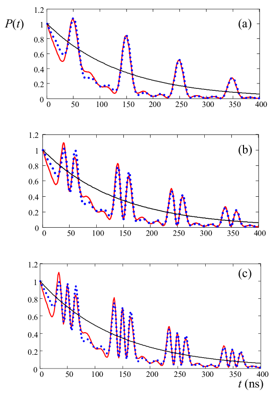
Figure 1: (color on line) Time dependence of the detection probability of a photon, $P(t)$, at the exit of the absorber vibrating with the frequency $\Omega=10$ MHz and phase $\varphi=0$. Optical thickness of the absorber is $T=5.2$ and $\gamma_{a}=\gamma_{s}=1.13$ MHz. The frequency of the radiation field $\omega_{s}$ is tuned in resonance with the first sideband $\omega_{a}+\Omega$ (a), the second sideband $\omega_{a}+2\Omega$ (b), and the third sideband $\omega_{a}+3\Omega$ (c). The value of the modulation index is taken optimal in each case, i.e., $p_{1}=1.8$ (a), $p_{2}=3.1$ (b), and $p_{3}=4.2$ (c), (see the text). Dotted line (in blue) corresponds to the analytical approximation (5) and solid line (in red) demonstrates the result obtained from the exact solution (6).

$$P(t)=\Theta(t)e^{-2\gamma t}\left[1+2S_{m}(t)\cos\psi_{m}(t)+S_{m}^{2}(t)\right],$$ (5)

where $\gamma=\gamma_{a}=\gamma_{s}$ and $\psi_{m}(t)=m(\Omega t+\varphi)-p\sin(\Omega t+\varphi)$. Time evolution of the probability $P(t)$ for $m=1$, $2$, and $3$, is shown in Fig. 1 (a, b, and c, respectively) where the results of approximate Eq. (5) are compared with the exact expression $P_{ext}(t)=\left|a_{ext}\right|^{2}$, which is obtained if we calculate the probability amplitude without any assumptions (see, for example, Ref. Ikonen ), i.e.,

$$a_{ext}(t,l)=a_{A}(t,l)-b{\displaystyle\int\limits_{0}^{t}}a_{A}(t-\tau,l)j_{1}(b\tau)e^{-\gamma_{a}\tau-i\omega_{a}\tau}d\tau,$$ (6)

where $j_{1}(b\tau)=J_{1}\left(2\sqrt{b\tau}\right)/\sqrt{b\tau}$. Small misfits can be almost excluded if we take into account the contribution of the two neighboring satellites, both red and blue detuned from the resonant component of the comb, see Supplemental Material (SM).

We see that the shape of the photon wave packet is transformed into bunches of pulses with the number of pulses per bunch equal to $m$. The pulses are produced due to constructive interference of the incident field with coherently scattered field when $\psi_{m}(t)=(2n+1)\pi$, $n=0,1,2,...$, while the dark windows appear due to destructive interference when $\psi_{m}(t)=2n\pi$, if $S_{m}(t)$ is negative in both cases. The probability has maxima, corresponding to pulses, $[1-S_{m}(t)]^{2}\exp(-2\gamma t)$ and minima $[1+S_{m}(t)]^{2}\exp(-2\gamma t)$, relevant to the radiation drop. The most pronounced pulses appear if the intensity of the resonant component [$\sim J_{m}^{2}(p)$] has global extremum. For example, the maxima, predicted by Eq. (5) without exponential factor $\exp(-2\gamma t)$ and assuming that $J_{0}\left(2\sqrt{bt}\right)\approx 0$, which means that the scattered field had time to fully develop, are $[1+J_{1}(p_{1})]^{2}=2.5$ if $p_{1}=1.8$; $[1+J_{2}(p_{2})]^{2}=2.1$ if $p_{2}=3.1$; and $[1+J_{3}(p_{3})]^{2}=2.06$ if $p_{3}=4.2$, i.e., the intensity of the pulses exceeds almost two times the intensity of the radiation field if it would not interact with the absorber. The radiation field between bunches is quite small because of destructive interference, for example, $[1-J_{1}(p_{1})]^{2}=0.175$ if $p_{1}=1.8$; $[1-J_{2}(p_{2})]^{2}=0.26$ if $p_{2}=3.1$; and $[1-J_{3}(p_{3})]^{2}=0.32$ if $p_{3}=4.2$, i.e., almost an order of magnitude smaller with respect to the pulse maxima. Qualitatively the appearance of bunches can be understood from the time evolution analysis of the phase difference of the scattered field and the comb, which is $\psi_{m}(t)+\pi$ if $S_{m}(t)<0$. The phase $\psi_{m}(t)$ evolves almost linearly as $(m+p)\Omega t+C$ during the pulse (pulses) formation around $\Omega t_{p}=(2n+1)\pi$ ($C$ is constant within each time interval), and the phase evolution almost stops around $\Omega t_{s}=2n\pi$, see SM for details.

It is interesting to notice that tuning in resonance the $m=-1$ component (if $\varphi=0$) shifts the position of the pulses with respect to the case of $m=+1$ such that maxima become minima and vice versa. Such a difference is explained by the fact that the amplitude of the $m=-1$ component of the comb is proportional to $J_{-1}(p)=-J_{1}(p)$ and hence the amplitude of the antiphase scattered field [proportional to $S_{-1}(t)$] becomes positive. The details how to move the radiation field from one time-bin to the other time-bin by changing the phase $\varphi$ and how this effect can be used to create time-bin qubits and qudits are discussed in SM.

Experiment. The details of the experimental setup are described in Refs. Shakhmuratov09 ; Shakhmuratov11 . Recently we developed a new scheme of photon counts selection and reported our first observation of photon shaping into a series of short single-pulse bunches Vagizov . This transformation is performed by tuning the radiation source in resonance with the first sideband $m=1$. Below we sketch out the experimental scheme.

The radiation source is a radioactive ⁵⁷Co in rhodium matrix. The absorber is a 25-$\mu$m-thick stainless-steel foil with a natural abundance ($\sim$ 2%) of ⁵⁷Fe. Optical depth of the absorber is $T_{a}=5.18$. The stainless-steel foil is glued on the polyvinylidene fluoride piezo-transducer that transforms the sinusoidal signal from radio-frequency generator into the uniform vibration of the foil. The tuning of the source in resonance for the preselected component of the spectrum is performed by Mössbauer transducer working/running in constant velocity mode. The source is attached to the holder of the Mössbauer transducer causing Doppler shift of the radiation field. Two detectors, D1 and D2, are used in data acquisition scheme. D1 (shielded by copper foil) detects only heralding 122 keV photons in a cascade decay, 122 keV and 14.4 keV, of ⁵⁷Co. This detector starts the clock. Detection of 14.4 keV photon by D2 stops the clock. In this time-delayed coincidence count technique we reconstruct the time evolution of the photon wave packet transmitted through the resonant absorber. Since time $t_{0}$ of the formation of 14.4 keV state nucleus in the source is random, we select only those counts of the heralding 122 keV photons, which are detected within short time interval $\Delta t$ around time $t_{ph}$ satisfying the relation $\Omega t_{ph}=\varphi+2\pi n$, where $n$ is integer. This selection secures that the phase of the absorber vibration is always the same for all detected photons. Since small time window of count selection $\Delta t$ is not zero, we have to average the theoretical expressions for the signal $P(t)$ over small jitter $\Delta\varphi$ of phase $\varphi$ caused by finite value of $\Delta t$.

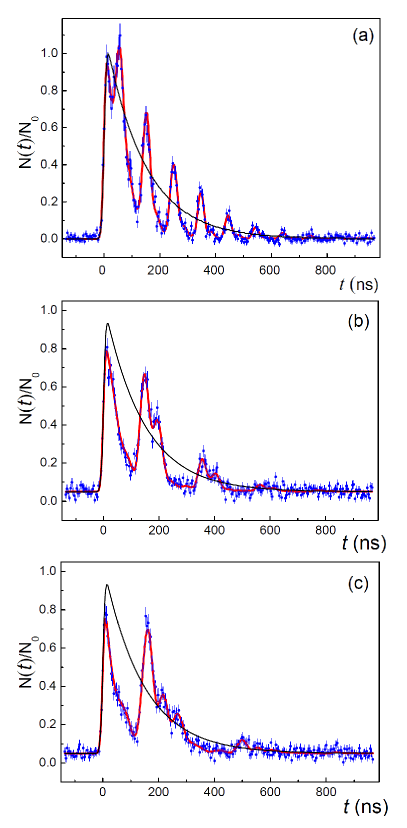
Figure 2: (color on line) Time dependence of the photon counts $N(t)$ at the exit of the absorber vibrating with the frequency $\Omega=10.2$ MHz (a), $\Omega=4.79$ MHz (b), and $\Omega=2.94$ MHz (c). $N(t)$ is normalized to the value $N_{0}$ without resonant absorbtion if the contribution of nonresonant photons with recoil is subtracted. The frequency of the radiation field $\omega_{s}$ is tuned in resonance with the first sideband $\omega_{a}+\Omega$ (a), the second sideband $\omega_{a}+2\Omega$ (b), and the third sideband $\omega_{a}+3\Omega$ (c). Solid line (in red) corresponds to the theoretical fitting, which takes into account the phase jitter. The modulation index, the phase, and the phase jitter $\Delta\varphi$ are $p=1.8$, $\varphi=0$, and $\Delta\varphi=\pi/2$ (a), $p=3.08$, $\varphi=0$, and $\Delta\varphi=\pi/3$ (b), $p=4.21$, $\varphi=-\pi/10$, and $\Delta\varphi=\pi/5$ (c). The dots with error bars (in blue) show experimental points. Thin line (in black) shows the probability time dependence without absorber.

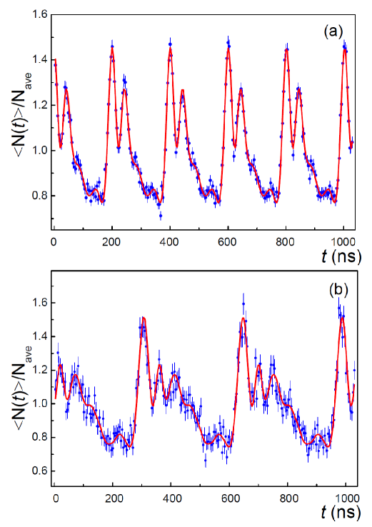
Figure 3: Time dependence of the $t_{0}$ averaged detection probability of a photon, $\langle N(t)\rangle\sim\langle P(t)\rangle_{t_{0}}$, at the exit of the vibrating absorber. $N_{ave}$ is the averaged count rate. The experimental conditions and notations in plots (a) and (b) are the same as in plots (b) and (c) in Fig. 2, respectively. The experimental results are fitted to the exact calculation of the integral in Eq. (7), see the details in SM.

Time resolution of the electronics in our setup is 8 ns and hence time structures shorter than 8 ns would be not resolved. In Ref. Vagizov we modulated the absorber with frequency $\Omega=10.2$ MHz and tuned the radiation field in resonance with the first satellite. We observed pulses as short as 30 ns, which are artificially broadened due to $\Delta\varphi\neq 0$. If we tune the source in resonance with the second or third satellite and keep the same frequency of modulation $\Omega=10.2$ MHz, the pulses will be 2 or 3 times shorter, respectively (see Fig. 1), which makes difficult to resolve pulses within the bunches. To be able to resolve the content of the pulse bunches, for example, consisting of two or three pulses, we had to reduce $\Omega$ two or three times, respectively, compared to the modulation frequency, used in our first experiment. The experimental results of the detecting of pulse bunching are presented in Fig. 2, where time dependence of the number of counts $N(t)$, normalized to the maximum value $N_{0}$ without absorber, is shown. The ratio $N(t)/N_{0}$ is proportional to the probability $P(t)$. The details of fitting procedure are described in Ref. Vagizov .

To avoid smearing out of the pulses within the bunch we performed experiments where time $t_{0}$ is still random but we count time delay of 14.4 keV photon detection by the detector D2 with respect to the fixed moments of time when the modulation phase $\varphi$ is the same (differing only in $2\pi n$). Thus, we don’t use detector D1 and time delay of the detection of 14.4 keV photon, $t_{stop}$, is counted with respect to a fixed $t_{start}$, which is not random. In this way we escape an artificial phase jitter $\Delta\varphi$ inherent to the first scheme of the experiment. What we measure in the modified scheme of experiment is the probability $P(t)$, integrated over time $t_{0}$, which varies from $-\infty$ to $t$, i.e.,

$$\left\langle P(t-t_{0})\right\rangle_{t_{0}}=2\gamma_{s}{\displaystyle\int\limits_{-\infty}^{t}}P(t-t_{0})dt_{0}.$$ (7)

Calculation of this integral for the analytical approximation, Eq. (5), gives

$$\left\langle P(t)\right\rangle_{t_{0}}=1-2V_{m}(p)\cos\psi_{m}(t)+U_{m}(p),$$ (8)

where $V_{m}(p)=J_{m}(p)[1-\exp(-T_{a}/4)]$, $U_{m}(p)=V_{m}^{2}(p)+J_{m}^{2}(p)\exp(-T_{a}/2)[I_{0}(T_{a}/2)-1]$, and $I_{0}(T_{a}/2)$ is the modified Bessel function of zero order. We notice that for a single line absorber (not vibrating) a steady state transmission of resonant gamma-quanta is proportional to the function $\exp(-T_{a}/2)I_{0}(T_{a}/2)$, where $T_{a}$ is the optical depth of the absorber. Therefore, we conclude that part of the term $U_{m}(p)$, which is proportional to this function, describes in Eq. (8) a steady state transmission of the resonant $m$-component of the frequency comb, within the assumption that other components pass through without any change. The exact expression for $\left\langle P(t-t_{0})\right\rangle_{t_{0}}$, obtained without analytical approximation (5), looks very complicated and does not allow simple interpretation and analytical analysis, see Ref. Ikonen . Meanwhile, our approximation slightly deviates from this exact result. However, if the contribution of two neighboring sidebands, blue and red detuned from resonant component, are taken into account, then this difference becomes negligible (see SM).

Figure 3 demonstrates the results of our time-delayed measurements with respect to a fixed phase of the vibrations. In spite of poor time resolution of our electronics the pulses within bunches are clearly seen.

Concluding, we demonstrate a method how to shape single-photon wave packets into bunches of pulses by transmission through the vibrated single-line absorber. We control the number of pulses in a bunch and their timing by tuning the absorber to the proper radiation sideband induced by the absorber vibration.

This work was partially funded by the Russian Foundation for Basic Research (Grant No. 12-02-00263-a), the Program of Competitive Growth of Kazan Federal University funded by the Russian Government, the RAS Presidium Program Quantum Mesoscopic and Disordered Systems , the National Science Foundation (Grant No. PHY-1307346), and the Robert A. Welch Foundation (Award A-1261). We are grateful to Alexey Kalachev for the fruitful discussions.

References

- (1) N. Gisin, G. Ribordy, W. Tittel, and H. Zbinden, Rev. Mod. Phys. 74, 145 (2002).
- (2) J. Brendel, N. Gisin, W. Tittel, and H. Zbinden, Phys. Rev. Lett. 82, 2594 (1999).
- (3) I. Marcikic, H. de Riedmatten, W. Tittel, V. Scarani, H. Zbinden, and N. Gisin, Phys. Rev. A 66, 062308 (2002).
- (4) R.T. Thew, A. Acin, H. Zbinden, and N. Gisin, Phys. Rev. Lett. 93, 010503 (2004).
- (5) P. C. Humphreys, B. J. Metcalf, J. B. Spring, M. Moore, X.-M. Jin, M. Barbieri, W. S. Kolthammer, and I. A. Walmsley, Phys. Rev. Lett. 111, 150501 (2013)
- (6) J. M. Donohue, M. Agnew, J. Lavoie, and K.J. Resch, Phys. Rev. Lett. 111, 153602 (2013)
- (7) B.R. Nisbet-Jones, J. Dilley, A. Holleczek, O. Barter, A. Kuhn, New Journal of Physics 15, 053007 (2013).
- (8) Y.V. Radeonychev, V.A. Polovinkin, O. Kocharovskaya, Phys. Rev. Lett. 105, 183902 (2010).
- (9) V. A. Antonov, Y. V. Radeonychev, O. Kocharovskaya, Phys. Rev, A 88, 053849 (2013)
- (10) Yu.V. Shvydko, S.L. Popov, G.V. Smirnov, Sov. Phys. JETP Lett. 53, 217 (1991).
- (11) Yu. V. Shvyd’ko, T. Hertrich, U. van Bürck, E. Gerdau, O. Leupold, J. Metge, H. D. Rüter, S. Schwendy, G. V. Smirnov, W. Potzel, and P. Schindelmann, Phys. Rev. Lett. 77, 3232 (1996).
- (12) A. Palffy, C. H. Keitel, and J. Evers, Phys. Rev. Lett. 103, 197403 (2012).
- (13) W.T. Liao, A. Pálffy, and C. H. Keitel, Phys. Rev. Lett. 109, 017401 (2009).
- (14) G. V. Smirnov, U. van Bürck, J. Arthur, S. L. Popov, A. Q. R. Baron, A. I. Chumakov, S. L. Ruby, W. Potzel, and G. S. Brown, Phys. Rev. Lett. 77, 183 (1996).
- (15) F. Vagizov, V. Antonov, Y.V. Radeonychev, R.N. Shakhmuratov, and O. Kocharovskaya, Nature 508, 80 (2014).
- (16) P. Helisto, I. Tittonen, M. Lippmaa, and T. Katila, Phys. Rev. Lett. 66, 2037 (1991).
- (17) I. Tittonen, M. Lippmaa, P. Helisto, and T. Katila, Phys. Rev. B 47, 7840 (1993).
- (18) P. Helisto, E. Ikonen, T. Katila, W. Potzel, and K. Riski, Phys. Rev. B 30, 2345 (1984).
- (19) E. Ikonen, P. Helisto, T. Katila, and K. Riski, Phys. Rev. A 32, 2298 (1985).
- (20) P. Schindelmann, U. van Burck, W. Potzel, G. V. Smirnov, S. L. Popov, E. Gerdau, Yu. V. Shvyd ko, J. Jeschke, H. D. Ruter, A. I. Chumakov, and R. Ruffer, Phys. Rev. A 65, 023804 (2002).
- (21) R. N. Shakhmuratov, F. Vagizov, and O. Kocharovskaya, Phys. Rev. A 84, 043820 (2011).
- (22) R. N. Shakhmuratov, F. Vagizov, and O. Kocharovskaya, Phys. Rev. A 87, 013807 (2013).
- (23) R. N. Shakhmuratov, Phys. Rev. A 85, 023827 (2012).
- (24) F. J. Lynch, R. E. Holland, and M. Hamermesh, Phys. Rev. 120, 513 (1960).
- (25) B. Lounis, W.E. Moerner, Nature (London) 407, 491 (2000).
- (26) S. M. Harris, Phys. Rev. 124, 1178 (1961).
- (27) M. D. Crisp, Phys. Rev. A 1, 1604 (1970).
- (28) R.N. Shakhmuratov, F. Vagizov, J. Odeurs, and O. Kocharovskaya, Phys. Rev. A 80, 063805 (2009).