A light tracking system to measure structural deformations

Abstract

Light tracking systems have been used in recent years to study wandering phenomena in atmospheric optics. We propose to employ this technology in structural deformation sensing.

¹Centro de Investigaciones Ópticas (CONICET La Plata - CIC), C.C. 3, 1897 Gonnet, Argentina

²Departamento de Física, Facultad de Ciencias Exactas, Universidad Nacional de La Plata (UNLP), 1900 La Plata, Argentina

³Departamento de Ciencias Básicas, Facultad de Ingeniería, Universidad Nacional de La Plata (UNLP), 1900 La Plata, Argentina

1 Introduction

Light tracking systems have been used for years to study phenomena in atmospheric optics [1, 2, 3, 4, 5]. For example, behavior of spot wandering variance versus pupil diameter in a laser propagation experiment is related to the structure constant ($C_{n}^{2}$) of the refractive index of air. In this situation it is very important to have a high precision spot tracking system with high sampling and recording frequency [7]. This technology has been used in structural applications in the past [6]. In this article we describe an application of this system to measure sectional deformations in structures. Available electronics components are detailed in Appendix A.

2 Basic setup

Suppose a long tubular of length $L$ and radius $R$ ($\sim$1.2 m in LIGO) structure suffering sectional types of deformation. Suppose section $A$ is fixed and has a laser emitting with a proper focusing system (see Fig. 1). The registering station is fixed at section $B$ (distance $L$) and both light trackers are centered.

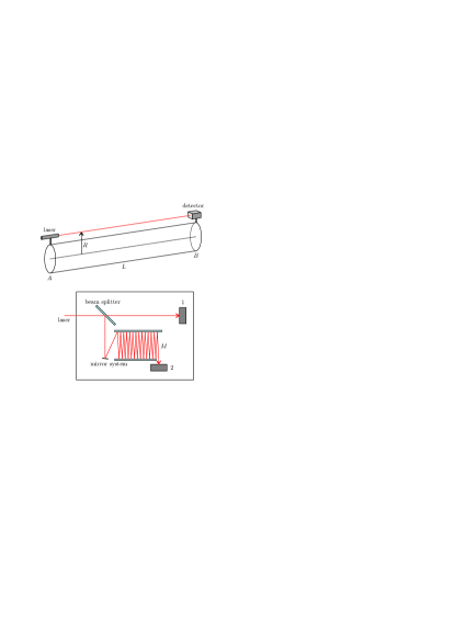
Figure 1: Basic setup and detector configuration. $M$ is the traveling distance of light from the beam splitter to light tracker 2 after a system of mirrors (optical distance multiplier).

2.1 $\varphi$-rotation

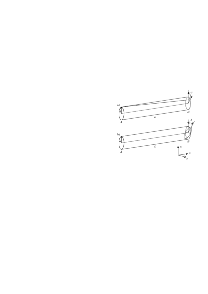
Figure 2: Sectional rotational deformations.

If section $B$ rotates an angle $\Delta\varphi$ relative to section $A$ (see Fig. 2-a), light tracker 1 will regard it as a horizontal displacement $\Delta x$. Since $\Delta x\cong R\Delta\varphi$:

$$\Delta\varphi\cong\frac{\Delta x}{R}$$ (1)

In an ideal case, the smallest possible measurable displacement is $\Delta x=2.54\cdot 10^{-6}\mbox{ m}$. Let’s assume that uncertainty in $R=1.2\mbox{ m}$ is $\delta R=R/100$ ($\delta$ means the error). Propagating errors (assuming $\Delta\varphi=0$) we find that

$$\delta\left(\Delta\varphi\right)\simeq\delta\left(\frac{\Delta x}{R}\right)\simeq 2.117\cdot 10^{-6}\mbox{ rad}$$

Light tracker 2 will see it as an opposite and equal horizontal displacement with a vertical component depending on traveling distance $M$.

2.1.1 Comment: rotation around $y$ axis

Suppose section $B$ rotates an angle $\Delta\psi$ around $y$ axis. It will be seen by tracker 1 as a horizontal displacement and by tracker 2 as $M\times 2\Delta\psi$ in opposite direction.

2.2 $\theta$-rotation

If section $B$ rotates an angle $\Delta\theta$ relative to section $A$ (see Fig. 2-b), light tracker 2 will regard it as a vertical displacement of magnitude $M\times 2\Delta\theta$. Light tracker 1 will see it as an opposite vertical displacement.

2.3 Pure horizontal and vertical displacements

For pure $y$ axis displacements both light trackers will detect a vertical centroid displacement of the same magnitude.

For pure $x$ axis displacements both light trackers will detect a horizontal centroid displacement of the same magnitude but of opposite sign due to beam splitter reflection in the registering station.

3 Final remarks and analysis techniques

Given the quality of this measuring setup it is possible to measure an angular deviation from the laser station to the registering station as small as $2.117\cdot 10^{-9}\mbox{ rad}$ ($L=1\mbox{ km}$), as well as other angular deviations in high frequency and precision. Accuracy in other relative angular measurements can be greatly improved by the optical distance multiplier ($M$ distance).

As for the analysis of time series, our group has experience with wavelets [11], information theory quantifiers (complexity-entropy causality plane, etc.) [14, 13, 12] and multifractal detrended fluctuation analysis (MFDFA) [15].

 

Appendix A Appendix: Opotoelectronic system for laser beam spot position tracking

This system was developed and built at Laboratorio de Procesamiento Láser (CIOp). It captures laser beam spot centroid positions at high frequency [7] and records them to a PC. The system can be operated with a single detector or with two in paralell. Sampling rate for single-mode can be fixed up to 12000 samples/s and in dual-mode it can be fixed up to 6000 samples/s for each detector.

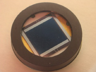
Figure 3: Continuous position detector.

A.1 Technical specs for continuous position detectors

A.1.1 SC-10D – Tetra-lateral

• Responsivity [9]:

  • min. 0.35 A/W.

  • typical 0.42 A/W.

• Active area: 103 $\mbox{mm}^{2}$.

• Dimensions: 10.16 mm $\times$ 10.16 mm.

• Max. power density: 10 $\mbox{mW/cm}^{2}$.

• Resolution: 0.00254 mm.

• VBias: up to -15V.

• Dark current:

  • typical 0.025 $\mu\mbox{A}$.

  • max. 0.250 $\mu\mbox{A}$.

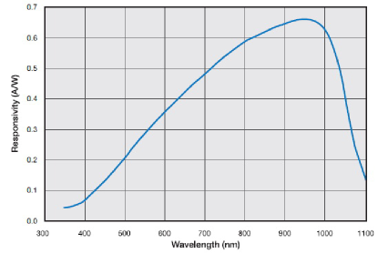
Figure 4: Typical spectral response for model SC-10D [9].

A.1.2 Model: DL-10 – Duo-lateral

• Responsivity [10]:

  • min. 0.3 A/W.

  • typical 0.4 A/W.

• Active area: 100 $\mbox{mm}^{2}$.

• Dimensions: 10 mm $\times$ 10 mm.

• Máx. power density: 1 $\mbox{mW/cm}^{2}$.

• Resolution: 0.00254 mm.

• VBias: -5V.

• Dark current:

  • typical 500 nA.

  • max. 5000 nA.

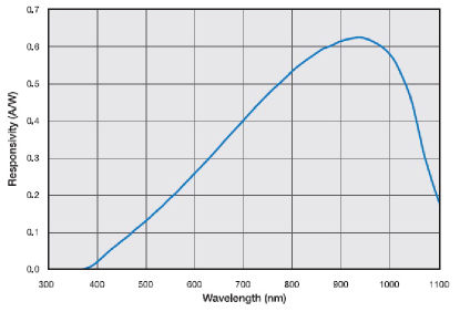
Figure 5: Typical spectral response for model DL-10 [10].

A.1.3 Data acquiring board NI-USB6009

Features [8]:

• 8 analog inputs, @ 14 bits and 48 kS/s. Differential mode and Single-ended.

• 2 analog outputs of 12 bits.

• 12 digital input/output lines.

• 32 bit counter, 5MHz.

• Digital trigger.

References

- [1] Andrews, L. C. & Phillips, R. L. (2005), Laser Beam Propagation through Random Media, Second Edition (SPIE Press Monograph Vol. PM152), SPIE Publications.
- [2] Gulich, M. Damián. (2011), Construcción y caracterización de un generador de turbulencias isotrópicas en aire caliente, Diploma work, Departamento de Física, Facultad de Ciencias Exactas, Universidad Nacional de La Plata.
- [3] Gulich, D.; Funes, G.; Zunino, L.; Pérez, D. G. & Garavaglia, M. (2006), ’Angle-of-arrival variance behavior and scale filtering in indoor turbulence’, Thirteenth Joint International Symposium on Atmospheric and Ocean Optics/ Atmospheric Physics 6522(1), in Gennadii G. Matvienko & Victor A. Banakh, ed., , SPIE, 65220L.
- [4] Gulich, D.; Funes, G.; Zunino, L.; Pérez, D. G. & Garavaglia, M. (2007), ’Angle-of-arrival variance’s dependence on the aperture size for indoor convective turbulence’, Optics Communications 277(2), 241 - 246.
- [5] Perez, D. G.; Zunino, L.; Gulich, D.; Funes, G. & Garavaglia, M. (2009), ’Turbulence characterization by studying laser beam wandering in a differential tracking motion setup’, Optics in Atmospheric Propagation and Adaptive Systems XII 7476(1), in Anton Kohnle; Karin Stein & John D. Gonglewski, ed., , SPIE, Congress: Optics in Atmospheric Propagation and Adaptive Systems XIIBerlin, Wednesday 2 September 2009, 74760D1-74760D8.
- [6] Cortizo, E. & Garavaglia, M (2005), ’Laser beam spot centroid detection and tracking: technological basis and a few applications’, 4ª Reunión Española de Optoelectrónica, OPTOEL’05 CI-3.
- [7] Rabal, S. (2010), Sistema Opto-electrónico para la Determinación de Posiciones, UNLP.
- [8] National Instruments, User guide and specifications - NI USB-6008/6009 Bus-Powered Multifunction DAQ USB Device, http://www.ni.com/pdf/manuals/371303m.pdf.
- [9] OSI Optoelectronics, Tetra Lateral Linear Photodiodes data sheet, http://www.osioptoelectronics.com/Libraries/Product-Data-Sheets/Tetra-Lateral-Linear-Photodiodes.sflb.ashx.
- [10] OSI Optoelectronics, Duo Lateral Linear Photodiodes data sheet, http://www.osioptoelectronics.com/Libraries/Product-Data-Sheets/Duo-Lateral-Linear-Photodiodes.sflb.ashx.
- [11] Zunino, L.; Pérez, D. G.; Garavaglia, M. & Rosso, O. A. (2007), ’Wavelet entropy of stochastic processes’, Physica A - Statistical And Theoretical Physics 379, 503 - 512.
- [12] Zunino, L.; Bariviera, A. F.; Guercio, M. B.; Martinez, L. B. & Rosso, O. A. (2012), ’On the efficiency of sovereign bond markets’, Physica A: Statistical Mechanics and its Applications 391(18), 4342 - 4349.
- [13] Zunino, L.; Tabak, B. M.; Serinaldi, F.; Zanin, M.; Pérez, D. G. & Rosso, O. A. (2011), ’Commodity predictability analysis with a permutation information theory approach’, Physica A: Statistical Mechanics and its Applications 390(5), 876 - 890.
- [14] Zunino, L.; Zanin, M.; Tabak, B. M.; Pérez, D. G. & Rosso, O. A. (2010), ’Complexity-entropy causality plane: A useful approach to quantify the stock market inefficiency’, Physica A: Statistical Mechanics and its Applications 389(9), 1891 - 1901.
- [15] Gulich, D. & Zunino, L. (2012), ’The effects of observational correlated noises on multifractal detrended fluctuation analysis’, Physica A: Statistical Mechanics and its Applications 391(16), 4100 - 4110.