Log-log Convexity of Type-Token Growth in Zipf’s Systems

Abstract

It is traditionally assumed that Zipf’s law implies the power-law growth of the number of different elements with the total number of elements in a system - the so-called Heaps’ law. We show that a careful definition of Zipf’s law leads to the violation of Heaps’ law in random systems, and obtain alternative growth curves. These curves fulfill universal data collapses that only depend on the value of the Zipf’s exponent. We observe that real books behave very much in the same way as random systems, despite the presence of burstiness in word occurrence. We advance an explanation for this unexpected correspondence.

A great number of systems in social science, economy, cognitive science, biology, and technology have been proposed to follow Zipf’s law Newman_05 ; Clauset ; Adamic_Huberman ; Furusawa2003 ; Axtell ; Serra_scirep . All of them have in common that they are composed by some “elementary” units, which we will call tokens, and that these tokens can be grouped into larger, concrete or abstract entities, called types. For instance, if the system is the population of a country, the tokens are its citizens, which can be grouped into different concrete types given by the cities where they live Malevergne_Sornette_umpu . If the system is a text, each appearance of a word is a token, associated to the abstract type given by the word itself Zanette_book . Zipf’s law deals with how tokens are distributed into types, and can be formulated in two different ways, which are generally considered as equivalent Newman_05 ; Adamic_Huberman ; Zanette_book ; Lu_2010 .

The first one is obtained when counting the number of tokens associated to each type, which are represented by their rank in the list of counts; if a (decreasing) power law holds between counts and ranks, with an exponent close to one, this indicates the fulfilment of Zipf’s law. The second version of the law arises when counting the number of types with a given value of the number of counts (this is the distribution of counts) and this yields a (decreasing) power law with exponent around two. However, in general, the fulfilment of Zipf’s law has not been tested with rigorous statistical methods Clauset ; Corral_Boleda ; rather, researchers have become satisfied with just qualitative resemblances between empirical data and power laws. In part, this can be justified by the difficulties of obtaining clear statistics from the rank-count representation, in particular for high ranks (that is, for rare types), and also by poor methods of estimation of probability distributions Clauset .

An important fact in most Zipf-like systems is that these present a temporal order. And whereas Zipf’s law reports a static property of these systems (as it is not altered under re-ordering of the data), a closely related statistics can unveil some of the dynamics. This is the type-token growth curve, which counts the number of types, $v$, as a function of the number of tokens, $\ell$, as a system evolves, i.e., as citizens are born or a text is being read. Note that $\ell$ is a measure of system size (as system grows) and $v$ is a measure of richness or diversity of types (with the symbol $v$ borrowed from linguistics, where it stands for the size of the vocabulary).

It has long been assumed that Zipf’s law implies also a power law for the type-token growth curve, i.e.,

$$v(\ell)\propto\ell^{\,\alpha},$$ (1)

with exponent $\alpha$ smaller than one, and this is referred to as Heaps’ law in general or Herdan’s law in quantitative linguistics Heaps_1978 ; Baeza_Yates00 ; Baayen . Indeed, Mandelbrot Mandelbrot61 and the authors of Ref. Leijenhorst_2005 obtain Heaps’ law when drawing independently tokens from a Zipf’s system. Baeza-Yates and Navarro Baeza_Yates00 argue that, if both Zipf’s law and Heaps’ law are fulfilled, their exponents are connected. A similar demonstration, using a different scaling of the variables, is found in Ref. Kornai2002 , and with some finite-size corrections in Ref. Lu_2010 . Other authors have been able to derive Heaps’ law from Zipf’s law using a master equation Serrano or pure scaling arguments FontClos_Corral . Alternatives to Heaps’ formula are listed in Ref. Wimmer_Altmann , but without a theoretical justification.

However, even simple visual inspection of the log-log plot of empirical type-token growth curves shows that Heaps’ law is not even a rough approximation of the reality. On the contrary, a clear convexity (as seen from above) is apparent in most of the plots (see, for instance, some of the figures in Lu_2010 ; Sano2012 ; Bernhardsson_2011 ). This has been attributed to the fact that the asymptotic regime is not reached or to the effects of the exhaustion of the number of different types Lu_2013 . Nevertheless, the effect persists in very large systems, composed by many millions of tokens, and where the finiteness of the number of available types is questionable FontClos_Corral .

In the few reported cases where there seems to be a true power-law relation between number of tokens and number of types, as in Ref. Kornai2002 , this turns out to come from a related but distinct statistics. Instead of considering the type-token growth curve in a single, growing system ($v(\ell)$ for $\ell=1\dots L$), one can look for the total type-token relationship in a collection or ensemble of $\mathcal{N}$ systems ($V_{j}$ versus $L_{j}$, for $j=1\dots\mathcal{N}$, with $V_{j}=v(L_{j})$), see also Refs. Serrano ; Petersen_scirep ; Gerlach_Altmann ; Gerlach . We are, in contrast, interested in the type-token relation of a single growing system.

The fact that Heaps’ law is so clearly violated for the type-token growth, given that this law follows directly from Zipf’s law, casts doubts on the very validity of the latter law. But one may notice that, although the two versions of Zipf’s law mentioned above are usually considered as equivalent, they are only asymptotically equivalent in the limit of very high counts Mandelbrot61 ; Heaps_1978 ; Baayen . However, the type-token growth curve emerges mainly from the statistics of the rarest types, for every $\ell$, as it is only when a type appears for the first time that it contributes to the growth curve FontClos_Corral , and these are precisely the types for which the usual description in terms of the rank-count representation becomes problematic. So, the election of which is the form of Zipf’s law that one considers to hold true becomes crucial for the derivation of the type-token growth curve and the fulfilment of Heaps’ law or not.

Although most previous research has focused in Zipf’s law in the rank-count representation, i.e., the first version mentioned above, we argue that it is the second version of the law, that of the distribution of counts, the one that becomes relevant to describe the real type-token growth curve, at least in the case of written texts. Indeed, let us notice that the previous derivations of Heaps’ law were all based on the rank-count representation Mandelbrot61 ; Leijenhorst_2005 ; Baeza_Yates00 ; Kornai2002 ; Lu_2010 ; Serrano ; FontClos_Corral ; therefore, the violation of Heaps’ law for real systems invalidates the (exact) fulfilment of Zipf’s law for the rank-count representation.

In contrast, when the viewpoint of Zipf’s law for the distribution of counts is adopted, we prove that Heaps’ law cannot be sustained for random systems and we derive an alternative law, which leads to “universal-like” shapes of the rescaled type-token growth curves, with the only dependence on the value of the Zipf’s exponent. Quite unexpectedly, our prediction for random uncorrelated systems holds very well also for real texts. We are able to explain this effect despite the significant clustering or burstiness of word occurrences Corral_words ; Motter , due to the special role that the first appearance in a text of a type plays, in contrast to subsequent appearances.

Let us consider a Zipf’s system of total size $L$, and a particular type with overall number of counts $n$; this means that the complete system contains $n$ tokens of that type (and then $L$ is the sum of counts of all types, $L=\sum_{i}n_{i}$). In fact, Zipf’s law tells us that there can be many types with the same counts $n$, and we denote this number as $N_{L}(n)$. Quantitatively, in terms of the distribution of counts, Zipf’s law reads

$$N_{L}(n)\propto\frac{1}{n^{\gamma}},$$ (2)

for $n=1,2,\dots$ with the exponent $\gamma$ close to 2. Note that $N_{L}(n)$ is identical, except for normalisation, to the probability mass function of the number of counts.

For a part of the system of size $\ell$, with $\ell\leq L$, the number of types with $k$ counts will be $N_{\ell}(k)$. The dependence of this quantity with the global $N_{L}(n)$ will be computed for a random system, which is understood as a sequence of tokens where these are taken at random from some underlying distribution. The $N_{L}(n)$ words with number of counts $n$ in the whole system will lead, on average, to $N_{L}(n)h_{k,n}$ types with counts $k$ in the subset, with $k\leq n$ and $h_{k,n}$ given by the hypergeometric distribution,

$$h_{k,n}=\frac{\binom{n}{k}\binom{L-n}{\ell-k}}{\binom{L}{\ell}}.$$ (3)

This is the probability to get $k$ instances of a certain type when drawing, without replacement, $\ell$ tokens from a total population of $L$ tokens of which there are $n$ tokens of the desired type. The dependence of $h_{k,n}$ on $\ell$ and $L$ is not explicit, to simplify the notation. The average number of types with $k$ counts in the subset of size $\ell$ will result from the sum of $N_{L}(n)h_{k,n}$ for all $n\geq k$, i.e.,

$$N_{\ell}(k)=\sum_{n\geq k}N_{L}(n)h_{k,n}.$$ (4)

We will use this relationship between $N_{\ell}(k)$ and $N_{L}(n)$ to derive the type-token growth curve.

For a subset of size $\ell$ we will have that, out of the total $V$ types, $v(\ell)$ will be present whereas $N_{\ell}(0)$ will not have appeared (and so, their number of counts will be $k=0$); therefore, $v(\ell)=V-N_{\ell}(0)$, and substituting Eq. (4) for $k=0$ and using that $N_{L}(0)=0$, then,

$$v(\ell)=V-\sum_{n\geq 1}N_{L}(n)h_{0,n}.$$ (5)

This formula relates the type-token growth curve with the distribution of counts in a random system, where it is exact, if we interpret $v(\ell)$ as an average over the random ensemble. We now show that a power-law distribution of type counts does not lead to a power law in the type-token growth curve, in other words, Zipf’s law for the distribution of counts does not lead to Heaps’ law, in the case of a random system.

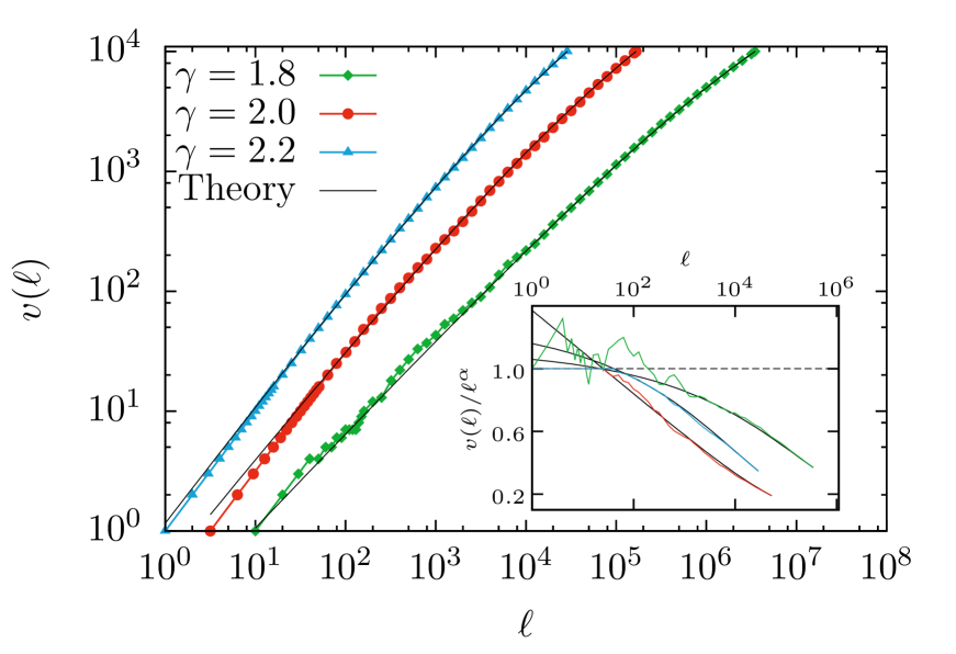
Figure 1: Main: Type-token growth curve $v(\ell)$ for three random systems with number of counts drawn from a discrete power-law distribution $N_{L}(n)\propto n^{-\gamma}$, and $\gamma=1.8$ (green diamonds), $2.0$ (red circles) and $2.2$ (blue triangles). The black lines correspond to our theoretical predictions, Eq. (8) for $\gamma\geq 2$ and Eq. (9) for $\gamma<2$ (plotted with the help of the GSL libraries). No average over the reshuffling procedure is performed. Curves are consecutively shifted by a factor of $\sqrt{1}0$ in the $x$-axis. Inset: The ratio $v(\ell)/\ell^{\alpha}$ is displayed, with $\alpha=\min\{1,\gamma-1\}$, showing that an approximation of the form $v(\ell)\propto\ell^{\alpha}$ is too crude.

First, taking advantage of a symmetry of the hypergeometric distribution and making an approximation for $n\ll L$, the “zero-success” probability $h_{0,n}$ turns out to be

$$h_{0,n}=\frac{\binom{L-n}{\ell}}{\binom{L}{\ell}}=\frac{\binom{L-\ell}{n}}{\binom{L}{n}}\simeq\left(1-\frac{\ell}{L}\right)^{n},$$

which in practice holds for all types; in fact, the smallest number of counts, for which the approximation is better, give the largest contribution to Eq. (5), due to the power-law form of $N_{L}(n)$. This is given, taking into account a normalisation constant $A$, by

$$N_{L}(n)=V\frac{A}{n^{\gamma}},$$ (6)

for $n=1,2,\dots$ (and zero otherwise), with $\sum_{n\geq 1}N_{L}(n)=V$. Let us substitute the previous expressions for $h_{0,n}$ and $N_{L}(n)$ into Eq. (5), then

$${}v(\ell)\simeq V\left(1-A\sum_{n\geq 1}\frac{(1-\ell/L)^{n}}{n^{\gamma}}\right).$$ (7)

Although there exists a maximum number of counts $n_{\max}$ beyond which $N_{L}(n)=0$, as a first approximation the sum can be safely extended up to infinity, and hence we reach the following expression:

$$v(\ell)\simeq V\left(1-\frac{\text{Li}_{\gamma}(1-\ell/L)}{\zeta(\gamma)}\right),\quad$$ (8)

where we have made use of the polylogarithm function, $\text{Li}_{\gamma}(z)=\sum_{n=1}^{\infty}{z^{n}}/{n^{\gamma}},$ defined for $|z|<1$, and of the fact that the normalisation of Zipf’s law is given by $A=1/\zeta(\gamma)$, with $\zeta(\gamma)$ the Riemann zeta function, $\zeta(\gamma)=\text{Li}_{\gamma}(1)$. Notice that, for random systems with fixed $\gamma$, Eq. (8) yields a “universal” scaling relationship between the number of types $v(\ell)$, if expressed in units of the total number of types $V$, and the text position $\ell$ expressed in units of the total size $L$.

In fact, Eq. (8) can lead to an overestimation of $v(\ell)$ due to finite-size effects, but this is rarely noticeable in practice. If one wants a more precise version of Eq. (8), then, going back to Eq. (7) and limiting the sum up to $n_{\max}$ gives, after some algebra,

$$v(\ell)=V\left(1-\frac{\text{Li}_{\gamma}(q)-q^{n_{\text{max}}+1}\Phi(q,\gamma,n_{\text{max}}+1)}{\zeta(\gamma)-\Phi(1,\gamma,n_{\text{max}}+1)}\right),$$ (9)

with $q=1-\ell/L$, and $\Phi(z,\gamma,a)=\sum_{n=0}^{\infty}\frac{z^{n}}{(a+n)^{\gamma}},\quad|z|<1;a\neq 0,-1,\dots$ the Lerch transcendent. Obviously, Eq. (9) gives better results at the cost of using an additional parameter, $n_{\max}$. As a rule of thumb, it appears to be worth the cost in cases where $\gamma<2$, $\ell\ll L$ and $L$ is not too large. In most practical cases Eq. (8) gives an excellent approximation; nevertheless, we include its more refined version, Eq. (9), for the sake of completeness.

In order to test these predictions, we simulate a random Zipf’s system as follows: Let us draw $V=10^{4}$ random numbers $n_{1},n_{2},\dots n_{V}$, from the discrete probability distribution $N_{L}(n)/V=n^{-\gamma}/\zeta(\gamma)$, with $\gamma=1.8,2.0$ and $2.2$. Each of these $V$ values of $n$ represents a type, with a number of counts given by the value of $n$. For each type $i=1,\dots,V$, we create then $n_{i}$ copies (tokens) of its associated type, and make a list with all of them,

$$\underbrace{1,\dots,1}_{n_{1}},\underbrace{2,\dots,2}_{n_{2}},\dots,\underbrace{V,\dots,V}_{n_{V}}.$$

Then, the list is reshuffled in order to create a random system, of size $L=n_{1}+n_{2}+\dots+n_{V}$. Figure 1 shows the resulting type-token growth together with the approximation given either by Eq. (8), which only depends on $\gamma$, or by Eq. (9), which depends on $\gamma$ and $n_{\text{max}}$. The agreement is nearly perfect, except for very small $\ell$.

So far we have shown that Eqs. (8) and (9) capture very accurately the type-token growth curve for synthetic systems that have a perfect power-law distribution of counts but are completely random. Real systems, however, can have richer structures beyond the distribution of counts Manning ; Corral_words ; Motter and so one wonders if our derivations can provide acceptable predictions for them.

In the following, we show that this is indeed the case when the system considered is that of natural language, and provide a qualitative explanation of this remarkable fact.

We analyse books from the Project Gutenberg (PG) database PG , selecting those whose distribution of frequencies $N_{L}(n)$ is statistically compatible with a pure, discrete power law distribution. We fit the $\gamma$ exponent with rigorous methods, see Refs. Corral_Deluca ; Corral_Deluca_arxiv ). In analogy with the previous section, we plot in Fig. 2 $v(\ell)/V$ versus $\ell/L$ for a total of 28 books for which $\gamma=1.8,2.0$, or $2.2$. Books with the same Zipf’s exponent collapse between them and into the corresponding theoretical curves, Eqs. (8) and (9). This is rather noticeable, as it points to the idea that the vocabulary-growth curve is unaffected by clustering, correlations, or by syntactic or discursive constraints. In other words, the vocabulary-growth curve of a real book fulfilling Zipf’s law as given by Eq. (2) is not a power law but can be predicted using only its associated Zipf’s exponent.

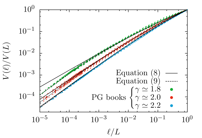
Figure 2: The rescaled vocabulary-growth curve of 28 books from the PG database with exponents $\gamma=\{1.8,2.0,2.2\}\pm 0.01$ fitted for $n\geq 1$ or $n\geq 2$. The values of $L$ and $V$ range from $27,873$ to $146,845$ and from $5,639$ to $30,912$ respectively. As it is apparent, all books with the same exponent collapse into a single curve, which Eqs. (8) and (9) accurately capture. For the case of Eq. (9), we have used a value of $n_{\max}/L=0.05$.

In order to understand why a prediction that heavily depends on the randomness hypothesis works so well for real books, we analyse the inter-occurrence-distance distribution of words. Given a word (type) with frequency $n$, we define its $k$-th inter-occurrence distance $\tau_{k}$ as the number of words (tokens) between its $k-1$-th and $k$-th appearances, plus one; i.e.,

$$\tau_{k}=\ell_{k}-\ell_{k-1}$$

(with $\ell_{k}$ the position of its $k$-th appearance and $k\leq n$). For the case of $k=1$, we compute the number of words from the beginning of the text up to the first appearance, i.e., $\tau_{1}=\ell_{1}$. If real books were completely random, then $\tau_{k}$ would be roughly exponentially distributed, and the rescaled distances

$$\hat{\tau}_{k}=\frac{\tau_{k}}{\langle\tau_{k}\rangle}$$ (10)

would be, for any value of $n$, exponentially distributed with parameter 1. Deviations from an exponential distribution for inter-occurrence distances in real books are well-known when all $k$ are considered together, and constitute the so-called clustering or burstiness effect: instances of a given word tend to appear grouped together in the book, forming clusters and hence both very short and very long inter-occurrence distances are much more common than what an exponential distribution predicts Corral_words ; Motter .

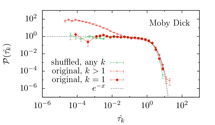
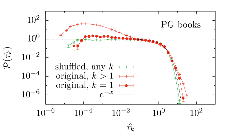
Figure 3: Distribution of the rescaled inter-occurrence distances $\hat{\tau}_{k}$, see Eq. (10). The scale parameter $\langle\tau_{k}\rangle$ was computed from the data of each book (types with $n=1$ or with $N(n)=1$ were not included in the analysis). The original books (red) display clear deviations from an exponential distribution for $k>1$, but not for $k=1$. Shuffled versions of the books (green) do not show, as expected, any clustering effect, and hence their rescaled inter-occurrence distances are roughly exponentially distributed. Top: The book Moby Dick, by Herman Melville, as an illustrative example. Bottom: The one hundred longest books in the PG database.

Our analysis introduces an additional element, the parameter $k$. Note that for what concerns the vocabulary-growth curve, all that matters is $k=1$, as it is only the first appearance of each word that adds to the vocabulary. Figure 3 shows the (estimated) probability mass function $\mathcal{P}(\hat{\tau}_{k})$ of the rescaled inter-occurrence distance for the book Moby Dick as an example (top), and for the one hundred longest books in the PG database (bottom). As it is apparent, for $k>1$, the distributions of distances are not exponentially distributed, and we recover a trace of the clustering effect; however the case $k=1$ displays a clearly different shape, much more close to an exponential distribution. This explains, at a qualitative level, why our derivations, based on a randomness assumption, continue to work in the case of real books that display clustering effects.

In conclusion, we have shown that Eqs. (8) and (9), which are not power laws but contain the polylogarithm function and the Lerch transcendent, provide a continuum of universality classes for type-token growth, depending only on Zipf’s exponent. We have verified our results both on synthetic random systems and on real books, showing that despite correlations or clustering effects, they remain valid as long as Zipf’s law is fulfilled. Our results open the door to investigations in other contexts beyond linguistics, where the validity of Heaps’ law could be questioned in a similar manner.

Acknowledgements. We have benefited from a long-term collaboration with G. Boleda and R. Ferrer-i-Cancho. Research projects in which this work is included are FIS2012-31324, from Spanish MINECO, and 2014SGR-1307, from AGAUR.

References

- (1) M. E. J. Newman. Power laws, Pareto distributions and Zipf’s law. Cont. Phys., 46:323 –351, 2005.
- (2) A. Clauset, C. R. Shalizi, and M. E. J. Newman. Power-law distributions in empirical data. SIAM Rev., 51:661–703, 2009.
- (3) L. A. Adamic and B. A. Huberman. Zipf’s law and the Internet. Glottometrics, 3:143–150, 2002.
- (4) C. Furusawa and K. Kaneko. Zipf’s law in gene expression. Phys. Rev. Lett., 90:088102, 2003.
- (5) R. L. Axtell. Zipf distribution of U.S. firm sizes. Science, 293:1818–1820, 2001.
- (6) J. Serrà, A. Corral, M. Boguñá, M. Haro, and J. Ll. Arcos. Measuring the evolution of contemporary western popular music. Sci. Rep., 2:521, 2012.
- (7) Y. Malevergne, V. Pisarenko, and D. Sornette. Testing the Pareto against the lognormal distributions with the uniformly most powerful unbiased test applied to the distribution of cities. Phys. Rev. E, 83:036111, 2011.
- (8) D. Zanette. Statistical Patterns in Written Language. 2012.
- (9) L. Lü, Z.-K. Zhang, and T. Zhou. Zipf’s law leads to Heaps’ law: Analyzing their relation in finite-size systems. PLoS ONE, 5(12):e14139, 12 2010.
- (10) A. Corral, G. Boleda, and R. Ferrer-i-Cancho. in preparation, 2013.
- (11) H. S. Heaps. Information retrieval: computational and theoretical aspects. Academic Press, 1978.
- (12) R. Baeza-Yates and G. Navarro. Block addressing indices for approximate text retrieval. J. Am. Soc. Inform. Sci., 51(1):69–82, 2000.
- (13) H. Baayen. Word Frequency Distributions. Kluwer, Dordrecht, 2001.
- (14) B. Mandelbrot. On the theory of word frequencies and on related Markovian models of discourse. In R. Jakobson, editor, Structure of Language and its Mathematical Aspects, pages 190–219. American Mathematical Society, Providence, RI, 1961.
- (15) D.C. van Leijenhorst and Th.P. van der Weide. A formal derivation of Heaps’ law. Inform. Sciences, 170:263 – 272, 2005.
- (16) A. Kornai. How many words are there? Glottom., 2:61–86, 2002.
- (17) M. A. Serrano, A. Flammini, and F. Menczer. Modeling statistical properties of written text. PLoS ONE, 4(4):e5372, 2009.
- (18) F. Font-Clos, G. Boleda, and A. Corral. A scaling law beyond Zipf’s law and its relation with Heaps’ law. New J. Phys., 15:093033, 2013.
- (19) G. Wimmer and G. Altmann. On vocabulary richness. J. Quant. Linguist., 6:1–9, 1999.
- (20) Y. Sano, H. Takayasu, and M. Takayasu. Zipf’s law and Heaps’ law can predict the size of potential words. Prog. Theor. Phys. Supp., 194:202–209, 2012.
- (21) S. Bernhardsson, S. K. Baek, and P. Minnhagen. A paradoxical property of the monkey book. J. Stat. Mech., 2011(07):P07013, 2011.
- (22) L. Lü, Z.-K. Zhang, and T. Zhou. Deviation of Zipf’s and Heaps’ Laws in human languages with limited dictionary sizes. Sci. Rep., 3:1–7, 2013.
- (23) A. M. Petersen, J. N. Tenenbaum, S. Havlin, H. E. Stanley, and M. Perc. Languages cool as they expand: Allometric scaling and the decreasing need for new words. Sci. Rep., 2:943, 2012.
- (24) M. Gerlach and E. G. Altmann. Stochastic model for the vocabulary growth in natural languages. Phys. Rev. X, 3:021006, 2013.
- (25) M. Gerlach and E. G. Altmann. Scaling laws and fluctuations in the statistics of word frequencies. New J. Phys., 16(11):113010, 2014.
- (26) A. Corral, R. Ferrer-i-Cancho, and A. Díaz-Guilera. Universal complex structures in written language. http://arxiv.org, 0901.2924, 2009.
- (27) E. G. Altmann, J. B. Pierrehumbert, and A. E. Motter. Beyond word frequency: Bursts, lulls, and scaling in the temporal distributions of words. ArXiv, 0901.2349v1, 2009.
- (28) C. D. Manning and H. Schütze. Foundations of Statistical Natural Language Processing. MIT Press, Cambridge, Massachusetts, 1999.
- (29) http://www.gutenberg.org/.
- (30) A. Deluca and A. Corral. Fitting and goodness-of-fit test of non-truncated and truncated power-law distributions. Acta Geophys., 61:1351–1394, 2013.
- (31) A. Corral, A. Deluca, and R. Ferrer-i-Cancho. A practical recipe to fit discrete power-law distributions. ArXiv, 1209:1270, 2012.