\DOIsuffix

theDOIsuffix \VolumeVV \IssueI \MonthMM \YearYYYY \pagespan3 \ReceiveddateXXXX \ReviseddateXXXX \AccepteddateXXXX \DatepostedXXXX

A thermodynamically consistent phenomenological model for ferroelectric and ferroelastic hysteresis

Barbara Kaltenbacher111e-mail: barbara.kaltenbacher@aau.at 11 Institute for Mathematics, Alpen-Adria-Universität, Universitätsstr. 65-67, A-9020 Klagenfurt, Austria    Pavel Krejčí 222e-mail: krejci@math.cas.cz 22 Institute of Mathematics, Czech Academy of Sciences, Žitná 25, CZ-11567 Praha 1, Czech Republic
Abstract.

We propose a hysteretic model for electromechanical coupling in piezoelectric materials, with the strain and the electric field as inputs and the stress and the polarization as outputs. This constitutive law satisfies the thermodynamic principles and exhibits good agreement with experimental measurements. Moreover, when it is coupled with the mechanical and electromagnetic balance equations, the resulting PDE system is well-posed under the hypothesis that hysteretic effects take place only in one preferred direction. We prove the existence and uniqueness of its global weak solutions for each initial data with prescribed regularity. One of the tools is a new Lipschitz continuity theorem for the inverse Preisach operator with time dependent coefficients.

keywords:
piezoelectricity, hysteresis operators, ferroelectrics, ferroelasticity
msc2010 Mathematics Subject Classification:
82D45, 35Q74, 35Q60
Supported by GAČR Grant P201/10/2315 and RVO: 67985840, as well as FWF grant P24970

1. Introduction

The piezoelectric effect is a coupling between electrical and mechanical fields within certain materials that has numerous applications ranging from ultrasound generation in medical imaging and therapy via acceleration sensors and injection valves in automotive industry to high precision positioning systems. Driven by the increasing demand for devices operating at high field intensities especially in actuator applications, the field of hysteresis modeling for piezoelectric materials is currently one of highly active research. The approaches that have been considered so far can be divided into basically four categories:

  1. (1)

    Thermodynamically consistent models being based on a macroscopic view to describe microscopic phenomena in such a way that the second law of thermodynamics is satisfied, see for example, Bassiouny and Ghaleb [3], Kamlah and Böhle [17], Landis [25], Schröder and Romanowski [34], Su and Landis [37], Linnemann et al. [26].

  2. (2)

    Micromechanical models that consider the material on the level of single grains, see, for example, Delibas et al. [9], Fröhlich [10], Huber and Fleck [13], Belov and Kreher [4], Huber [12], McMeeking et al. [28], Smith and Hu [35].

  3. (3)

    Phase field models that describe the transition between phases (corresponding to the motion of walls between domains with different polarization orientation) using the Ginzburg-Landau equation for some order parameter, see, for example Xu et al [40], Wang et al [39].

  4. (4)

    Phenomenological models using hysteresis operators partly originating from the input-output description of piezoelectric devices for control purposes, see, for example, Hughes and Wen [14], Kuhnen [24], Cima et al. [7], Smith et al. [36], Ball et al. [2], Pasco and Berry [31].

Also multiscale coupling between macro- and microscopic as well as phase field models partly even down to atomistic simulations has been investigated, see, e.g., [29, 33].

For a mathematical analysis of some thermodynamically consistent models we refer to [1, 19, 30].

Whereas most of the so far existing models are designed for the simulation of polarization, depolarization or cycling along the main hysteresis loop, the simulation of actuators requires the accurate simulation of minor loops as well. Moreover, the physical behavior can so far be reproduced only qualitatively, whereas the use of models in actuator simulation (possibly also aiming at simulation based optimization) needs to match measurements precisely. Simulation of a piezoelectric device with a possibly complex geometry requires not only an input-output model but needs to resolve the spatial distribution of the crucial electric and mechanical field quantities, which leads to partial differential equations. Therewith, the question of numerical efficiency becomes important.

Preisach operators [5, 18, 22, 27, 38] are phenomenological models for rate independent hysteresis that are capable of reproducing minor loops and can be very well fitted to measurements. Moreover, they allow for a highly efficient evaluation by the application of certain memory deletion rules and the use of so-called Everett or shape functions.

Motivated by these facts, in [11, 15], a model for ferroelectric hysteresis under uniaxial loading using Preisach operators is proposed and studied. Like most of the above mentioned models, it is based on an additive decomposition of the strain and the polarization into reversible and irreversible parts. The reversible quantities follow the linear piezoelectric material law, while the irreversible polarization is represented by a Preisach operator of the imposed electric field and the irreversible strain is a polynomial function of the polarization. Moreover, the piezoelectric coupling coefficient is proportional to the polarization.

However, for the model from [11, 15], it is not clear whether or under which conditions the second law of thermodynamics is satisfied. We will therefore here consider a new material law, which is inspired by the one proposed for magnetostriction [8] whose thermodynamic consistency is based on the use of hysteresis potentials, and which is additionally able to capture ferroelastic effects.

The paper is structured as follows. In Section 2, we derive piezoelectric constitutive equations involving a Preisach hysteresis operator from basic thermodynamic principles and show some simulation results with the proposed model. Section 3 is devoted to the proof of a new result on Lipschitz invertibility of the Preisach operator with time dependent coefficients, and in Section 4 we construct a unique solution of a system of electromechanical balance equations by Banach contraction principle. We restrict ourselves to the situation of uniaxial loading, hence scalar constitutive relations. A perspective to the situation of electric and mechanic fields depending on three space variables while still considering uniaxial loading, is provided in Section 5. The case of vector or actually tensor valued hysteresis will be subject of future research.

2. The model

Differently from most of the above cited approaches, we consider the electric field E𝐸E and the mechanical strain ε𝜀\varepsilon as state variables and the dielectric displacement D=D(ε,E)𝐷𝐷𝜀𝐸D=D(\varepsilon,E) as well as the mechanical stress σ=σ(ε,E)𝜎𝜎𝜀𝐸\sigma=\sigma(\varepsilon,E) as state functions. The reason for doing so lies in the fact that the balance equations

(namely Newton’s law on the mechanical side and Gauss law on the electric side)

ρu¨sTσ𝜌¨𝑢superscriptsubscript𝑠𝑇𝜎\displaystyle\rho\ddot{u}-\nabla_{s}^{T}\sigma =\displaystyle= 00\displaystyle 0 (1)
D𝐷\displaystyle-\nabla\cdot D =\displaystyle= 00\displaystyle 0 (2)

(where u𝑢u is the mechanical displacement, ssubscript𝑠\nabla_{s} the symmetric gradient and sTsuperscriptsubscript𝑠𝑇\nabla_{s}^{T} the dyadic divergence) are naturally formulated in terms of these state functions.

For the interrelation between these quantities, we assume, similarly to [8], that hysteresis effects are due to one single Preisach operator 𝒫𝒫{\mathcal{P}} with potential 𝒰𝒰{\mathcal{U}} acting on an auxiliary state function q=q(ε,E)𝑞𝑞𝜀𝐸q=q(\varepsilon,E). In the scalar case, this leads to the assumption that the stress σ𝜎\sigma, the dielectric displacement D𝐷D, and the free energy F=F(ε,E)𝐹𝐹𝜀𝐸F=F(\varepsilon,E) are of the form

σ𝜎\displaystyle\sigma =\displaystyle= c¯εeE+a𝒫[q]+b𝒰[q],¯𝑐𝜀𝑒𝐸𝑎𝒫delimited-[]𝑞𝑏𝒰delimited-[]𝑞\displaystyle\underline{c}\varepsilon-eE+a{\mathcal{P}}[q]+b{\mathcal{U}}[q], (3)
D𝐷\displaystyle D =\displaystyle= eε+κE+c𝒫[q]+d𝒰[q],𝑒𝜀𝜅𝐸𝑐𝒫delimited-[]𝑞𝑑𝒰delimited-[]𝑞\displaystyle e\varepsilon+\kappa E+c{\mathcal{P}}[q]+d{\mathcal{U}}[q], (4)
F𝐹\displaystyle F =\displaystyle= c¯2ε2+κ2E2+ξ𝒫[q]+η𝒰[q],¯𝑐2superscript𝜀2𝜅2superscript𝐸2𝜉𝒫delimited-[]𝑞𝜂𝒰delimited-[]𝑞\displaystyle\frac{\underline{c}}{2}\varepsilon^{2}+\frac{\kappa}{2}E^{2}+\xi{\mathcal{P}}[q]+\eta{\mathcal{U}}[q], (5)

where the coefficients a=a(ε,E)𝑎𝑎𝜀𝐸a=a(\varepsilon,E), b=b(ε,E)𝑏𝑏𝜀𝐸b=b(\varepsilon,E), c=c(ε,E)𝑐𝑐𝜀𝐸c=c(\varepsilon,E), d=d(ε,E)𝑑𝑑𝜀𝐸d=d(\varepsilon,E), ξ=ξ(ε,E)𝜉𝜉𝜀𝐸\xi=\xi(\varepsilon,E), η=η(ε,E)𝜂𝜂𝜀𝐸\eta=\eta(\varepsilon,E) as well as the function q=q(ε,E)𝑞𝑞𝜀𝐸q=q(\varepsilon,E), are to be determined in agreement with the principles of thermodynamics. The elastic, dielectric, and piezoelectric coupling coefficients c¯>0¯𝑐0\underline{c}>0, e𝑒absente\in\real, and κ>0𝜅0\kappa>0 are given constants. It will be shown in Section 3 that the Preisach hysteresis operator with nonnegative density satisfies the energy inequality

q(t)ddt𝒫[q](t)ddt𝒰[q](t)0 a.e. qW1,1(0,T).formulae-sequence𝑞𝑡dd𝑡𝒫delimited-[]𝑞𝑡dd𝑡𝒰delimited-[]𝑞𝑡0 a.e. for-all𝑞superscript𝑊110𝑇q(t)\frac{\,\mathrm{d}}{\,\mathrm{d}t}{\mathcal{P}}[q](t)-\frac{\,\mathrm{d}}{\,\mathrm{d}t}{\mathcal{U}}[q](t)\geq 0\ \mbox{ a.e. }\quad\forall q\in W^{1,1}(0,T). (6)

Similarly to Section 3.4 in [8], we now derive conditions to ensure thermodynamic admissibility, namely the requirement that

ε˙σ+D˙EF˙0˙𝜀𝜎˙𝐷𝐸˙𝐹0\dot{\varepsilon}\sigma+\dot{D}E-\dot{F}\geq 0 (7)

has to hold for all processes ε𝜀\varepsilon, σ𝜎\sigma, D𝐷D, E𝐸E that obey the constitutive laws (3), (4). We obtain

0(aε˙+Ec˙ξ˙)𝒫[q]+(bε˙+Ed˙η˙)𝒰[q]+(Ecξ)ddt𝒫[q]+(Edη)ddt𝒰[q].0𝑎˙𝜀𝐸˙𝑐˙𝜉𝒫delimited-[]𝑞𝑏˙𝜀𝐸˙𝑑˙𝜂𝒰delimited-[]𝑞𝐸𝑐𝜉dd𝑡𝒫delimited-[]𝑞𝐸𝑑𝜂dd𝑡𝒰delimited-[]𝑞0\leq(a\dot{\varepsilon}+E\dot{c}-\dot{\xi}){\mathcal{P}}[q]+(b\dot{\varepsilon}+E\dot{d}-\dot{\eta}){\mathcal{U}}[q]+(Ec-\xi)\frac{\,\mathrm{d}}{\,\mathrm{d}t}{\mathcal{P}}[q]\\ +(Ed-\eta)\frac{\,\mathrm{d}}{\,\mathrm{d}t}{\mathcal{U}}[q]\,. (8)

Both 𝒫[q]𝒫delimited-[]𝑞{\mathcal{P}}[q] and 𝒰[q]𝒰delimited-[]𝑞{\mathcal{U}}[q] are hysteresis operators and may take arbitrary values independent of each other, so that we have to demand

0=0absent\displaystyle 0= aε˙+Ec˙ξ˙=ε˙(a+Ecεξε)+E˙(EcEξE),𝑎˙𝜀𝐸˙𝑐˙𝜉˙𝜀𝑎𝐸𝑐𝜀𝜉𝜀˙𝐸𝐸𝑐𝐸𝜉𝐸\displaystyle\ a\dot{\varepsilon}+E\dot{c}-\dot{\xi}=\dot{\varepsilon}\left(a+E\frac{\partial c}{\partial\varepsilon}-\frac{\partial\xi}{\partial\varepsilon}\right)+\dot{E}\left(E\frac{\partial c}{\partial E}-\frac{\partial\xi}{\partial E}\right), (9)
0=0absent\displaystyle 0= bε˙+Ed˙η˙=ε˙(b+Edεηε)+E˙(EdEηE).𝑏˙𝜀𝐸˙𝑑˙𝜂˙𝜀𝑏𝐸𝑑𝜀𝜂𝜀˙𝐸𝐸𝑑𝐸𝜂𝐸\displaystyle\ b\dot{\varepsilon}+E\dot{d}-\dot{\eta}=\dot{\varepsilon}\left(b+E\frac{\partial d}{\partial\varepsilon}-\frac{\partial\eta}{\partial\varepsilon}\right)+\dot{E}\left(E\frac{\partial d}{\partial E}-\frac{\partial\eta}{\partial E}\right).

These relations have to hold for all processes, hence the coefficients of ε˙˙𝜀\dot{\varepsilon} and E˙˙𝐸\dot{E} have to vanish identically. In other words, if we set f1=ηEdsubscript𝑓1𝜂𝐸𝑑f_{1}=\eta-Ed, f2=Ecξsubscript𝑓2𝐸𝑐𝜉f_{2}=Ec-\xi, we must have

a=f2ε,b=f1ε,c=f2E,d=f1E.formulae-sequence𝑎subscript𝑓2𝜀formulae-sequence𝑏subscript𝑓1𝜀formulae-sequence𝑐subscript𝑓2𝐸𝑑subscript𝑓1𝐸a=-\frac{\partial f_{2}}{\partial\varepsilon},\ b=\frac{\partial f_{1}}{\partial\varepsilon},\ c=\frac{\partial f_{2}}{\partial E},\ d=-\frac{\partial f_{1}}{\partial E}. (10)

Inequality (8) then becomes

0f2ddt𝒫[q]f1ddt𝒰[q],0subscript𝑓2dd𝑡𝒫delimited-[]𝑞subscript𝑓1dd𝑡𝒰delimited-[]𝑞0\leq f_{2}\frac{\,\mathrm{d}}{\,\mathrm{d}t}{\mathcal{P}}[q]-f_{1}\frac{\,\mathrm{d}}{\,\mathrm{d}t}{\mathcal{U}}[q]\,, (11)

and will be satisfied, by virtue of (6), provided we choose q:=f2/f1assign𝑞subscript𝑓2subscript𝑓1q:=f_{2}/f_{1} with f1>0subscript𝑓10f_{1}>0.

We see that the whole model depends on the choice of two state functions f1=f1(ε,E)>0subscript𝑓1subscript𝑓1𝜀𝐸0f_{1}=f_{1}(\varepsilon,E)>0 and f2=f2(ε,E)subscript𝑓2subscript𝑓2𝜀𝐸f_{2}=f_{2}(\varepsilon,E) which characterize the material properties. A canonical choice, which is sufficient in many situations, consists in putting f2(ε,E)=Esubscript𝑓2𝜀𝐸𝐸f_{2}(\varepsilon,E)=E, f1(ε,E)=f(ε)subscript𝑓1𝜀𝐸𝑓𝜀f_{1}(\varepsilon,E)=f(\varepsilon) with a suitable function f𝑓f of one variable. Then the constitutive law (3)–(5) becomes

σ𝜎\displaystyle\sigma =\displaystyle= c¯εeE+f(ε)𝒰[Ef(ε)],¯𝑐𝜀𝑒𝐸superscript𝑓𝜀𝒰delimited-[]𝐸𝑓𝜀\displaystyle\underline{c}\varepsilon-eE+f^{\prime}(\varepsilon){\mathcal{U}}\left[\frac{E}{f(\varepsilon)}\right], (12)
D𝐷\displaystyle D =\displaystyle= eε+κE+𝒫[Ef(ε)],𝑒𝜀𝜅𝐸𝒫delimited-[]𝐸𝑓𝜀\displaystyle e\varepsilon+\kappa E+{\mathcal{P}}\left[\frac{E}{f(\varepsilon)}\right], (13)
F𝐹\displaystyle F =\displaystyle= c¯2ε2+κ2E2+f(ε)𝒰[Ef(ε)].¯𝑐2superscript𝜀2𝜅2superscript𝐸2𝑓𝜀𝒰delimited-[]𝐸𝑓𝜀\displaystyle\frac{\underline{c}}{2}\varepsilon^{2}+\frac{\kappa}{2}E^{2}+f(\varepsilon){\mathcal{U}}\left[\frac{E}{f(\varepsilon)}\right]. (14)

The full 1D system for unknown functions u(x,t)𝑢𝑥𝑡u(x,t), E(x,t)𝐸𝑥𝑡E(x,t), (x,t)(0,)×(0,T)𝑥𝑡00𝑇(x,t)\in(0,\ell)\times(0,T), describing longitudinal oscillations of a piezoelectric beam, then reads

ρuttσx=𝜌subscript𝑢𝑡𝑡subscript𝜎𝑥absent\displaystyle\rho u_{tt}-\sigma_{x}= 0,0\displaystyle\ 0, (15)
Dx=subscript𝐷𝑥absent\displaystyle D_{x}= 0,0\displaystyle\ 0,
ε=𝜀absent\displaystyle\varepsilon= ux.subscript𝑢𝑥\displaystyle\ u_{x}.

The equation Dx=0subscript𝐷𝑥0D_{x}=0 means that D𝐷D is a function of t𝑡t only, say, D(x,t)=r(t)𝐷𝑥𝑡𝑟𝑡D(x,t)=r(t), that is,

eε+κE+𝒫[Ef(ε)]=r(t),𝑒𝜀𝜅𝐸𝒫delimited-[]𝐸𝑓𝜀𝑟𝑡e\varepsilon+\kappa E+{\mathcal{P}}\left[\frac{E}{f(\varepsilon)}\right]=r(t)\,, (16)

where r(t)𝑟𝑡r(t) is a function which is known from the boundary condition D(0,t)=D(,t)=r(t)𝐷0𝑡𝐷𝑡𝑟𝑡D(0,t)=D(\ell,t)=r(t), corresponding to an impressed (or measured) boundary current. Furthermore, we complement the mechanical constitutive law (12) with a viscosity term νεt𝜈subscript𝜀𝑡\nu\varepsilon_{t}, where ν>0𝜈0\nu>0 is the viscosity coefficient, that is,

σ𝜎\displaystyle\sigma =\displaystyle= νεt+c¯εeE+f(ε)𝒰[Ef(ε)]𝜈subscript𝜀𝑡¯𝑐𝜀𝑒𝐸superscript𝑓𝜀𝒰delimited-[]𝐸𝑓𝜀\displaystyle\nu\varepsilon_{t}+\underline{c}\varepsilon-eE+f^{\prime}(\varepsilon){\mathcal{U}}\left[\frac{E}{f(\varepsilon)}\right] (17)

instead of (12). We prescribe some boundary conditions, for example u=0𝑢0u=0 on x=0𝑥0x=0, and σ=s(t)𝜎𝑠𝑡\sigma=s(t) on x=𝑥x=\ell, which corresponds to the experimental setting of a beam which is clamped at the left tip, with an impressed (or measured) force at the right beam tip. We resume the analysis of this system in Section 4 and before, in Section 3, we establish some new properties of the Preisach operator which will enable us to eliminate E𝐸E from the system by solving Eq. (16) independently with respect to q=E/f(ε)𝑞𝐸𝑓𝜀q=E/f(\varepsilon).

\remarkname 2.1

We wish to mention that independence of the dielectric saturation value on the stress (which is the case e.g. for the setting c=1𝑐1c=1, d=0𝑑0d=0 considered in Section 3.4.1 of [8]) physically makes sense also here: Note that saturation of the polarization, i.e., of P=𝒫[q]𝑃𝒫delimited-[]𝑞P={\mathcal{P}}[q] taking its maximal absolute value, corresponds to the situation of all c-axes (and therewith all elementary dipoles) of the single crystals being aligned as much as possible to the load axis, under the given geometric constraints (note that each grain has its own coordinate system of preferred directions). This maximal alignment gives the same polarization, independent of the imposed stress. In other words, no matter how large the imposed stress is, there exists a sufficiently large impressed electric field (in load axis direction) that will bring the polarization to its maximal value by aligning all elementary dipoles (and therewith all c-axes) as much as possible in load direction.

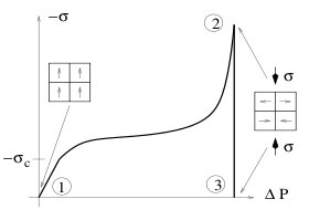
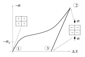
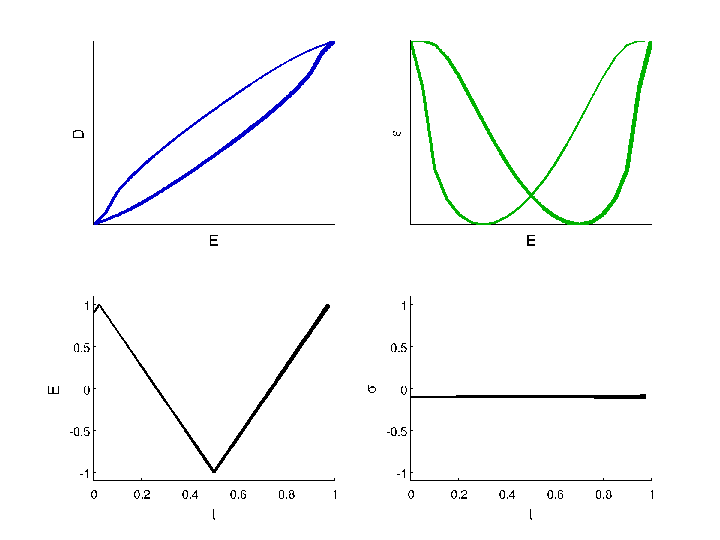
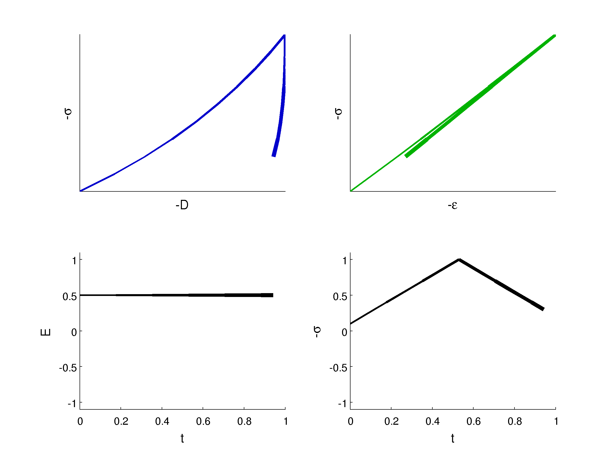
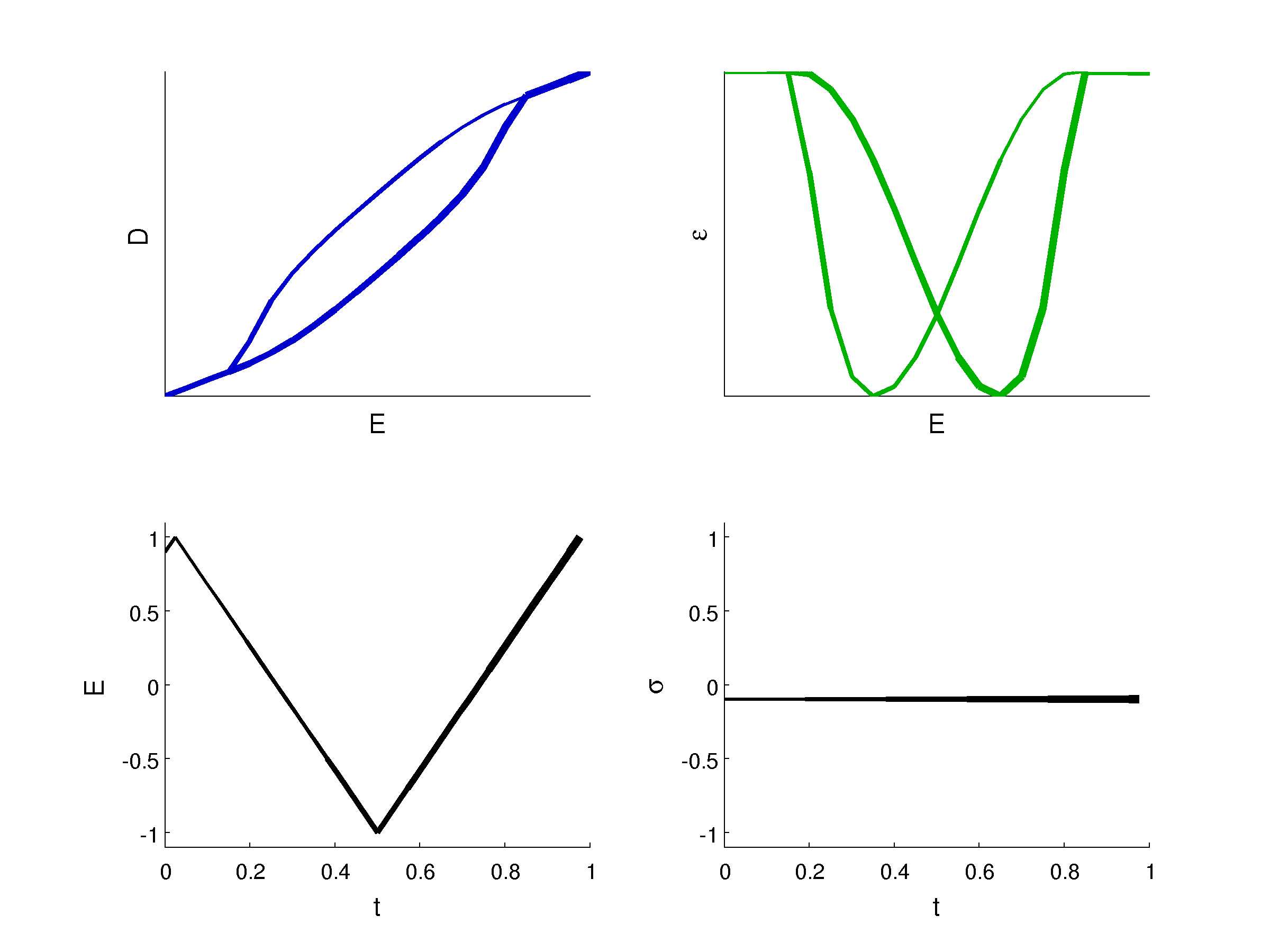
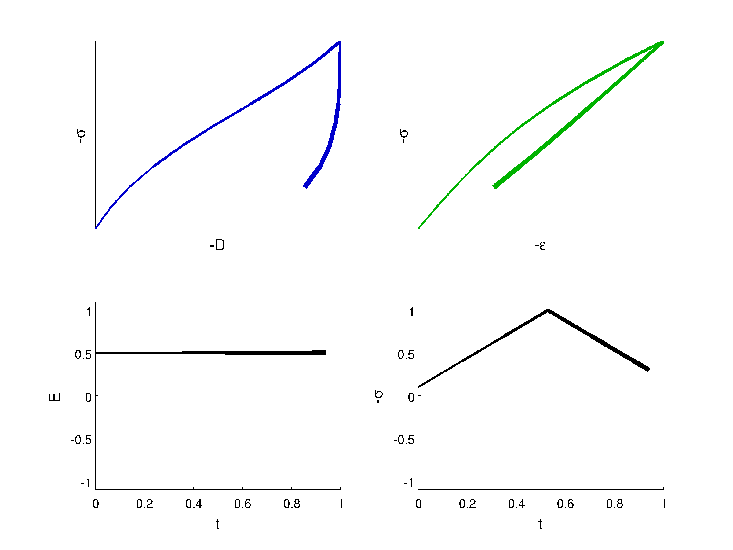
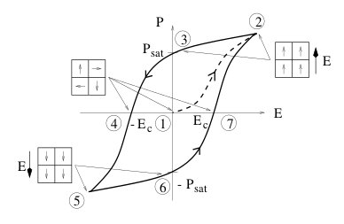
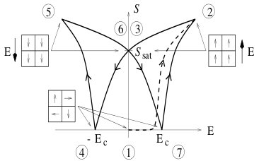
We conclude this section with some simulation results for a very simple choice of the Preisach operator 𝒫𝒫{\mathcal{P}} and the function f𝑓f, see Figures 3, 4, 5, 6, in order to illustrate that the expected qualitative behavior of ferroelectric and ferroelastic hysteresis (see Figures 1, 2 taken from [16]) can indeed be recovered. Here we use the functions

g(r,s)={proj[1+r,1r](s)=max{1+r,min{1r,s}} if r10 else 𝑔𝑟𝑠casessubscriptproj1𝑟1𝑟𝑠1𝑟1𝑟𝑠 if 𝑟1otherwise0 else otherwiseg(r,s)=\begin{cases}\mbox{proj}_{[-1+r,1-r]}(s)=\max\{-1+r,\min\{1-r,s\}\}\mbox{ if }r\leq 1\\ 0\mbox{ else }\end{cases} (18)

in the Definition 3.2 of 𝒫𝒫{\mathcal{P}}, as well as

f(x)=1.1x1x1formulae-sequence𝑓𝑥1.1𝑥1𝑥1f(x)=1.1-x\,\quad-1\leq x\leq 1 (19)

or

f(x)=12+(x1)441x1formulae-sequence𝑓𝑥12superscript𝑥1441𝑥1f(x)=\frac{1}{2}+\frac{(x-1)^{4}}{4}\,\quad-1\leq x\leq 1 (20)

(in both cases the extension to [1,1]11\real\setminus[-1,1] is done such that Hypothesis 3.3 is satisfied) c¯=1¯𝑐1\underline{c}=1, e=0𝑒0e=0, κ=0.01𝜅0.01\kappa=0.01 in (14), and normalize all input quantities to the unit interval [1,1]11[-1,1]. In Figures 3, 4, 5, 6,increasing line thickness indicates proceeding time in order to show that the curves are traversed in the right direction.
Of course, also quantitative agreement with measurement can be expected to be achievable by approprate fitting methods.
Refer to caption
Refer to caption
Figure 1. polarization hysteresis (left) and strain (butterfly) hysteresis (right) under a bipolar electric field excitation; taken from [16]
Refer to caption
Refer to caption
Figure 2. mechanical depolarization (left) and stress-strain relation (right) under compressive stress load; taken from [16]
Refer to caption
Figure 3. polarization hysteresis (top row left) and strain (butterfly) hysteresis (top row right) under a bipolar electric field excitation (bottom row); simulations with model (14) where f𝑓f is chosen according to (19), and 𝒫𝒫{\mathcal{P}} according to Definition 3.2 with (18).
Refer to caption
Figure 4. mechanical depolarization (left) and stress-strain relation (right) under compressive stress load (bottom row); simulations with model (14) where f𝑓f is chosen according to (19), and 𝒫𝒫{\mathcal{P}} according to Definition 3.2 with (18).
Refer to caption
Figure 5. polarization hysteresis (top row left) and strain (butterfly) hysteresis (top row right) under a bipolar electric field excitation (bottom row); simulations with model (14) where f𝑓f is chosen according to (20), and 𝒫𝒫{\mathcal{P}} according to Definition 3.2 with (18).
Refer to caption
Figure 6. mechanical depolarization (left) and stress-strain relation (right) under compressive stress load (bottom row); simulations with model (14) where f𝑓f is chosen according to (20), and 𝒫𝒫{\mathcal{P}} according to Definition 3.2 with (18).

3. Inversion of hysteresis operators with time dependent coefficients

In this section, we prove Lipschitz continuity statements for mappings which with given functions w,bC[0,T]𝑤𝑏𝐶0𝑇w,b\in C[0,T] associate the solution q𝑞q of the equation

q(t)+b(t)𝒫[q](t)=w(t)t[0,T],formulae-sequence𝑞𝑡𝑏𝑡𝒫delimited-[]𝑞𝑡𝑤𝑡for-all𝑡0𝑇q(t)+b(t){\mathcal{P}}[q](t)=w(t)\quad\forall t\in[0,T]\,, (21)

where 𝒫:C[0,T]C[0,T]:𝒫𝐶0𝑇𝐶0𝑇{\mathcal{P}}:C[0,T]\to C[0,T] is a Lipschitz continuous operator in the sense that

|𝒫[q1](t)𝒫[q2](t)|Mmaxτ[0,t]|q1(τ)q2(τ)|𝒫delimited-[]subscript𝑞1𝑡𝒫delimited-[]subscript𝑞2𝑡𝑀subscript𝜏0𝑡subscript𝑞1𝜏subscript𝑞2𝜏|{\mathcal{P}}[q_{1}](t)-{\mathcal{P}}[q_{2}](t)|\leq M\max_{\tau\in[0,t]}|q_{1}(\tau)-q_{2}(\tau)| (22)

for some M>0𝑀0M>0 and for all q1,q2C[0,T]subscript𝑞1subscript𝑞2𝐶0𝑇q_{1},q_{2}\in C[0,T].

It follows from (22) that 𝒫𝒫{\mathcal{P}} has the Volterra property, i.e., for all t[0,T]𝑡0𝑇t\in[0,T]

q1,q2C[0,T]:q1=q2 on [0,t] implies 𝒫[q1]=𝒫[q2] on [0,t].\forall q_{1},q_{2}\in C[0,T]\ :\quad q_{1}=q_{2}\mbox{ on }[0,t]\mbox{ implies }{\mathcal{P}}[q_{1}]={\mathcal{P}}[q_{2}]\mbox{ on }[0,t]\,.

We first specify sufficient conditions under which is the mapping (w,b)qmaps-to𝑤𝑏𝑞(w,b)\mapsto q well defined.

\lemmaname 3.1

Let 𝒫𝒫{\mathcal{P}} be as in (22), and such that I+c𝒫𝐼𝑐𝒫I+c{\mathcal{P}} admits for every c0𝑐0c\geq 0 a Lipschitz continuous inverse in the sense that the inequality

|(I+c𝒫)1[w1](t)(I+c𝒫)1[w2](t)|Lmaxτ[0,t]|w1(τ)w2(τ)|superscript𝐼𝑐𝒫1delimited-[]subscript𝑤1𝑡superscript𝐼𝑐𝒫1delimited-[]subscript𝑤2𝑡𝐿subscript𝜏0𝑡subscript𝑤1𝜏subscript𝑤2𝜏|(I+c{\mathcal{P}})^{-1}[w_{1}](t)-(I+c{\mathcal{P}})^{-1}[w_{2}](t)|\leq L\max_{\tau\in[0,t]}|w_{1}(\tau)-w_{2}(\tau)| (23)

holds for all q1,q2C[0,T]subscript𝑞1subscript𝑞2𝐶0𝑇q_{1},q_{2}\in C[0,T] with Lipschitz constant L>0𝐿0L>0 independent of c𝑐c. Let w,bC[0,T]𝑤𝑏𝐶0𝑇w,b\in C[0,T] be given functions, and let b(t)0𝑏𝑡0b(t)\geq 0 for all t[0,T]𝑡0𝑇t\in[0,T]. Then there exists a unique qC[0,T]𝑞𝐶0𝑇q\in C[0,T] such that (21) holds.

The Lipschitz continuity of (I+c𝒫)1superscript𝐼𝑐𝒫1(I+c{\mathcal{P}})^{-1} independently of the constant c𝑐c is fulfilled in many typical situations arising in the theory of hysteresis operators. If 𝒫𝒫{\mathcal{P}} is the Preisach operator defined below in Definition 3.2, it was shown in [6] that (23) is satisfied with L=2𝐿2L=2. If 𝒫𝒫{\mathcal{P}} belongs to the subclass of Prandtl-Ishlinskii operators, then (I+c𝒫)1superscript𝐼𝑐𝒫1(I+c{\mathcal{P}})^{-1} admits in addition an explicit representation, see [20].

  •     Proof.

    We choose γ<1/(ML)𝛾1𝑀𝐿\gamma<1/(ML) and a division 0=t0<t1<<tm=T0subscript𝑡0subscript𝑡1subscript𝑡𝑚𝑇0=t_{0}<t_{1}<\dots<t_{m}=T of [0,T]0𝑇[0,T] such that |b(t)b(tk1)|<γ𝑏𝑡𝑏subscript𝑡𝑘1𝛾|b(t)-b(t_{k-1})|<\gamma for t[tk1,tk]𝑡subscript𝑡𝑘1subscript𝑡𝑘t\in[t_{k-1},t_{k}], k=1,,m𝑘1𝑚k=1,\dots,m. We prove by induction that

    k{1,,m}!qC[0,tk]:q satisfies (21).\forall k\in\{1,\ldots,m\}\ \exists!q\in C[0,t_{k}]\ :\quad q\mbox{ satisfies \eqref{e1}}.

    In [0,t1]0subscript𝑡1[0,t_{1}], we rewrite (21) as

    q(t)+b(0)𝒫[q](t)=w(t)(b(t)b(0))𝒫[q](t),𝑞𝑡𝑏0𝒫delimited-[]𝑞𝑡𝑤𝑡𝑏𝑡𝑏0𝒫delimited-[]𝑞𝑡q(t)+b(0){\mathcal{P}}[q](t)=w(t)-(b(t)-b(0)){\mathcal{P}}[q](t)\,,

    or, equivalently,

    q(t)=(I+b(0)𝒫)1[w(b()b(0))𝒫[q]](t).𝑞𝑡superscript𝐼𝑏0𝒫1delimited-[]𝑤𝑏𝑏0𝒫delimited-[]𝑞𝑡q(t)=(I+b(0){\mathcal{P}})^{-1}\big{[}w-(b(\cdot)-b(0)){\mathcal{P}}[q]\big{]}(t)\,. (24)

    By our assumptions of Lipschitz continuity and the choice of γ𝛾\gamma, the mapping on the right hand side of (24) is a contraction with respect to q𝑞q, hence it admits a unique fixed point.

    Assume now that we have constructed a unique q(t)𝑞𝑡q(t) satisfying (21) on [0,tk1]0subscript𝑡𝑘1[0,t_{k-1}]. We introduce the set

    Vk={q^C[0,tk]:q^(t)=q(t) on [0,tk1]}.subscript𝑉𝑘conditional-set^𝑞𝐶0subscript𝑡𝑘^𝑞𝑡𝑞𝑡 on 0subscript𝑡𝑘1V_{k}=\{\hat{q}\in C[0,t_{k}]:\hat{q}(t)=q(t)\mbox{ on }[0,t_{k-1}]\}.

    We define a mapping Rk:VkVk:subscript𝑅𝑘subscript𝑉𝑘subscript𝑉𝑘R_{k}:V_{k}\to V_{k} which with each q^Vk^𝑞subscript𝑉𝑘\hat{q}\in V_{k} associates the solution q𝑞q of the equation

    q(t)+b(tk1)𝒫[q](t)=w(t)(b(t)b(tk1))𝒫[q^](t)𝑞𝑡𝑏subscript𝑡𝑘1𝒫delimited-[]𝑞𝑡𝑤𝑡𝑏𝑡𝑏subscript𝑡𝑘1𝒫delimited-[]^𝑞𝑡q(t)+b(t_{k-1}){\mathcal{P}}[q](t)=w(t)-(b(t)-b(t_{k-1})){\mathcal{P}}[\hat{q}](t) (25)

    for t[0,tk]𝑡0subscript𝑡𝑘t\in[0,t_{k}]. The mapping Rksubscript𝑅𝑘R_{k} is again a contraction on Vksubscript𝑉𝑘V_{k} (by our assumptions of Lipschitz continuity, the choice of γ𝛾\gamma, as well as the Volterra property) and therefore admits a unique fixed point. The induction argument over k𝑘k then completes the proof. ∎

Here, we focus on the case of Preisach operators. We use the following definition which is shown in [21] to be equivalent to the original Preisach construction in [32].

\definitionname 3.2

Let g:(0,)×g:(0,\infty)\times\real\to\real be a measurable function which is Lipschitz continuous in the second variable and such that g(r,0)=0𝑔𝑟00g(r,0)=0 for a. e. r>0𝑟0r>0. For a given input qW1,1(0,T)𝑞superscript𝑊110𝑇q\in W^{1,1}(0,T), we define the output 𝒫[q]W1,1(0,T)𝒫delimited-[]𝑞superscript𝑊110𝑇{\mathcal{P}}[q]\in W^{1,1}(0,T) of a Preisach operator 𝒫𝒫{\mathcal{P}} by the integral

𝒫[q](t)=0g(r,ξr(t))drfor t[0,T],formulae-sequence𝒫delimited-[]𝑞𝑡superscriptsubscript0𝑔𝑟subscript𝜉𝑟𝑡differential-d𝑟for 𝑡0𝑇{\mathcal{P}}[q](t)=\int_{0}^{\infty}g(r,\xi_{r}(t))\,\mathrm{d}r\quad\mbox{for }t\in[0,T]\,, (26)

where ξrW1,1(0,T)subscript𝜉𝑟superscript𝑊110𝑇\xi_{r}\in W^{1,1}(0,T) is the unique solution of the variational inequality

{|q(t)ξr(t)|rt[0,T],ξ˙r(t)(q(t)ξr(t)rz)0a. e. |z|1,ξr(0)=max{q(0)r,min{0,q(0)+r}}.cases𝑞𝑡subscript𝜉𝑟𝑡𝑟for-all𝑡0𝑇subscript˙𝜉𝑟𝑡𝑞𝑡subscript𝜉𝑟𝑡𝑟𝑧0a. e. for-all𝑧1subscript𝜉𝑟0𝑞0𝑟0𝑞0𝑟missing-subexpression\left\{\begin{array}[]{ll}|q(t)-\xi_{r}(t)|\leq r&\forall t\in[0,T]\,,\\ \dot{\xi}_{r}(t)(q(t)-\xi_{r}(t)-rz)\geq 0&\mbox{a.\,e. }\ \forall|z|\leq 1\,,\\ \xi_{r}(0)=\max\{q(0)-r,\min\{0,q(0)+r\}\}\,.&\end{array}\right. (27)

The Preisach operator 𝒫𝒫{\mathcal{P}} is called a Prandtl-Ishlinskii operator if g𝑔g is linear in v𝑣v, that is, g(r,v)=μ(r)v𝑔𝑟𝑣𝜇𝑟𝑣g(r,v)=\mu(r)v for some μLloc1(0,)𝜇subscriptsuperscript𝐿1𝑙𝑜𝑐0\mu\in L^{1}_{loc}(0,\infty).

We easily check from (27) that ξr(t)=0subscript𝜉𝑟𝑡0\xi_{r}(t)=0 for rq𝑟norm𝑞r\geq\|q\|, where \|\cdot\| denotes the sup-norm in C[0,T]𝐶0𝑇C[0,T], so that the integral in (26) is meaningful.

The parameter r𝑟r is the memory variable, and the mapping qξrmaps-to𝑞subscript𝜉𝑟q\mapsto\xi_{r} introduced in [18] is called the play operator. Note that its extension to C[0,T]𝐶0𝑇C[0,T] is Lipschitz continuous with Lipschitz constant 111, that is,

|ξr1(t)ξr2(t)|maxτ[0,t]|q1(τ)q2(τ)|.superscriptsubscript𝜉𝑟1𝑡superscriptsubscript𝜉𝑟2𝑡subscript𝜏0𝑡subscript𝑞1𝜏subscript𝑞2𝜏|\xi_{r}^{1}(t)-\xi_{r}^{2}(t)|\leq\max_{\tau\in[0,t]}|q_{1}(\tau)-q_{2}(\tau)|\,. (28)

For our purposes, it is convenient to reduce the set of admissible functions g𝑔g, and we adopt the following hypothesis.

Hypothesis 3.3

We assume that g(r,0)=0𝑔𝑟00g(r,0)=0 for a. e. r>0𝑟0r>0, and

  • (i)

    0gv(r,v)μ(r)0𝑔𝑣𝑟𝑣𝜇𝑟0\leq\frac{\partial g}{\partial v}(r,v)\leq\mu(r) a. e., where μL1(0,)𝜇superscript𝐿10\mu\in L^{1}(0,\infty), 0μ(r)dr=Msuperscriptsubscript0𝜇𝑟differential-d𝑟𝑀\int_{0}^{\infty}\mu(r)\,\mathrm{d}r=M;

  • (ii)

    There exists >M1>0subscript𝑀10\infty>M_{1}>0 such that

    0gv(r,v)dvdr=M1.superscriptsubscript0superscriptsubscript𝑔𝑣𝑟𝑣differential-d𝑣differential-d𝑟subscript𝑀1\int_{0}^{\infty}\int_{-\infty}^{\infty}\frac{\partial g}{\partial v}(r,v)\,\mathrm{d}v\,\mathrm{d}r=M_{1}. (29)

Hypothesis 3.3 (i) means that thr Preisach operator 𝒫𝒫{\mathcal{P}} is dominated by a Prandtl-Ishlinskii operator. Hypothesis 3.3 (ii) implies that 𝒫[q]M1norm𝒫delimited-[]𝑞subscript𝑀1\|{\mathcal{P}}[q]\|\leq M_{1} for all qC[0,T]𝑞𝐶0𝑇q\in C[0,T]. It is easy to check that even without Hypothesis 3.3 (i), (ii), the Preisach operator satisfies the energy inequality (6) with the choice

𝒰[q](t)=0G(r,ξr(t))dr,𝒰delimited-[]𝑞𝑡superscriptsubscript0𝐺𝑟subscript𝜉𝑟𝑡differential-d𝑟{\mathcal{U}}[q](t)=\int_{0}^{\infty}G(r,\xi_{r}(t))\,\mathrm{d}r\,, (30)

with

G(r,v)=0vvgv(r,v)dv.𝐺𝑟𝑣superscriptsubscript0𝑣superscript𝑣𝑔𝑣𝑟superscript𝑣differential-dsuperscript𝑣G(r,v)=\int_{0}^{v}v^{\prime}\frac{\partial g}{\partial v}(r,v^{\prime})\,\mathrm{d}v^{\prime}\,. (31)

Moreover, it satisfies the Volterra property by virtue of (28). Still by (28), the operator 𝒫𝒫{\mathcal{P}} can be extended to C[0,T]𝐶0𝑇C[0,T], and if Hypothesis 3.3 (i) is fulfilled, then the Lipschitz property (22) holds.

The main result of this section reads as follows.

\theoremname 3.4

Let Hypothesis 3.3 (i) hold, and let b,w1,w2C[0,T]𝑏subscript𝑤1subscript𝑤2𝐶0𝑇b,w_{1},w_{2}\in C[0,T] be given, 0b(t)b¯0𝑏𝑡¯𝑏0\leq b(t)\leq\bar{b} for all t[0,T]𝑡0𝑇t\in[0,T]. Let q1,q2C[0,T]subscript𝑞1subscript𝑞2𝐶0𝑇q_{1},q_{2}\in C[0,T] be such that

qi(t)+b(t)𝒫[qi](t)=wi(t)t[0,T],i=1,2.formulae-sequencesubscript𝑞𝑖𝑡𝑏𝑡𝒫delimited-[]subscript𝑞𝑖𝑡subscript𝑤𝑖𝑡formulae-sequencefor-all𝑡0𝑇𝑖12q_{i}(t)+b(t){\mathcal{P}}[q_{i}](t)=w_{i}(t)\quad\forall t\in[0,T]\,,\quad i=1,2\,. (32)

Then we have

q1q2eb¯Mw1w2.normsubscript𝑞1subscript𝑞2superscripte¯𝑏𝑀normsubscript𝑤1subscript𝑤2\|q_{1}-q_{2}\|\leq\mathrm{e}^{\bar{b}M}\|w_{1}-w_{2}\|\,. (33)

The proof of Theorem 3.4 is divided into several steps. Indeed, as W1,1(0,T)superscript𝑊110𝑇W^{1,1}(0,T) is dense in C[0,T]𝐶0𝑇C[0,T], it is enough to prove (33) for qiW1,1(0,T)subscript𝑞𝑖superscript𝑊110𝑇q_{i}\in W^{1,1}(0,T), and we repeatedly use the variational inequality (27). The following observation is due to Brokate, see [5], and is related to the Brokate identity in more general situations, cf. [23]. We give a full proof here, also because it uses techniques that will play a substantial role in the proof of Theorem 3.4.

\lemmaname 3.5

Let r2>r1>0subscript𝑟2subscript𝑟10r_{2}>r_{1}>0 and qW1,1(0,T)𝑞superscript𝑊110𝑇q\in W^{1,1}(0,T) be given, and let ξrisubscript𝜉subscript𝑟𝑖\xi_{r_{i}}, i=1,2𝑖12i=1,2, be the solution of (27). Then we have

{|ξr1(t)ξr2(t)|r2r1t[0,T],ξ˙r2(t)(ξr1(t)ξr2(t)(r2r1)z)0a. e. |z|1.casessubscript𝜉subscript𝑟1𝑡subscript𝜉subscript𝑟2𝑡subscript𝑟2subscript𝑟1for-all𝑡0𝑇subscript˙𝜉subscript𝑟2𝑡subscript𝜉subscript𝑟1𝑡subscript𝜉subscript𝑟2𝑡subscript𝑟2subscript𝑟1𝑧0a. e. for-all𝑧1\left\{\begin{array}[]{ll}|\xi_{r_{1}}(t)-\xi_{r_{2}}(t)|\leq r_{2}-r_{1}&\forall t\in[0,T]\,,\\ \dot{\xi}_{r_{2}}(t)(\xi_{r_{1}}(t)-\xi_{r_{2}}(t)-(r_{2}-r_{1})z)\geq 0&\mbox{a.\,e. }\ \forall|z|\leq 1\,.\end{array}\right. (34)
  •     Proof.

    Let ηW1,1(0,T)𝜂superscript𝑊110𝑇\eta\in W^{1,1}(0,T) be the solution of the variational inequality

    {|ξr1(t)η(t)|r2r1t[0,T],η˙(t)(ξr1(t)η(t)(r2r1)z)0a. e. |z|1η(0)=max{ξr1(0)(r2r1),min{0,ξr1(0)+(r2r1)}}.casessubscript𝜉subscript𝑟1𝑡𝜂𝑡subscript𝑟2subscript𝑟1for-all𝑡0𝑇˙𝜂𝑡subscript𝜉subscript𝑟1𝑡𝜂𝑡subscript𝑟2subscript𝑟1𝑧0a. e. for-all𝑧1𝜂0subscript𝜉subscript𝑟10subscript𝑟2subscript𝑟10subscript𝜉subscript𝑟10subscript𝑟2subscript𝑟1missing-subexpression\left\{\begin{array}[]{ll}|\xi_{r_{1}}(t)-\eta(t)|\leq r_{2}-r_{1}&\forall t\in[0,T]\,,\\ \dot{\eta}(t)(\xi_{r_{1}}(t)-\eta(t)-(r_{2}-r_{1})z)\geq 0&\mbox{a.\,e. }\ \forall|z|\leq 1\\ \eta(0)=\max\{\xi_{r_{1}}(0)-(r_{2}-r_{1}),\min\{0,\xi_{r_{1}}(0)+(r_{2}-r_{1})\}\}\,.&\end{array}\right. (35)

    Putting in the above inequality z=ξr1(t±δ)η(t±δ)r2r1𝑧subscript𝜉subscript𝑟1plus-or-minus𝑡𝛿𝜂plus-or-minus𝑡𝛿subscript𝑟2subscript𝑟1z=\frac{\xi_{r_{1}}(t\pm\delta)-\eta(t\pm\delta)}{r_{2}-r_{1}} and letting δ𝛿\delta tend to 0+limit-from00+ we obtain

    η˙(t)(ξ˙r1(t)η˙(t))=0a. e.˙𝜂𝑡subscript˙𝜉subscript𝑟1𝑡˙𝜂𝑡0a. e.\dot{\eta}(t)(\dot{\xi}_{r_{1}}(t)-\dot{\eta}(t))=0\quad\mbox{a.\,e.} (36)

    We have by (27) for r=r1𝑟subscript𝑟1r=r_{1} that ξ˙r1(t)(q(t)ξr1(t)r1z)0subscript˙𝜉subscript𝑟1𝑡𝑞𝑡subscript𝜉subscript𝑟1𝑡subscript𝑟1𝑧0\dot{\xi}_{r_{1}}(t)(q(t)-\xi_{r_{1}}(t)-r_{1}z)\geq 0 a. e. for all |z|1𝑧1|z|\leq 1, and (36) implies the implication η˙(t)0η˙(t)=ξ˙r1(t)˙𝜂𝑡0˙𝜂𝑡subscript˙𝜉subscript𝑟1𝑡\dot{\eta}(t)\neq 0\Longrightarrow\dot{\eta}(t)=\dot{\xi}_{r_{1}}(t). Hence,

    η˙(t)(q(t)ξr1(t)r1z)0a. e. |z|1.˙𝜂𝑡𝑞𝑡subscript𝜉subscript𝑟1𝑡subscript𝑟1𝑧0a. e. for-all𝑧1\dot{\eta}(t)(q(t)-\xi_{r_{1}}(t)-r_{1}z)\geq 0\ \mbox{a.\,e. }\ \forall|z|\leq 1. (37)

    We have |q(t)η(t)|r2𝑞𝑡𝜂𝑡subscript𝑟2|q(t)-\eta(t)|\leq r_{2}, and adding (37) to (35) we obtain

    η˙(t)(q(t)η(t)r2z)0a. e. |z|1.˙𝜂𝑡𝑞𝑡𝜂𝑡subscript𝑟2𝑧0a. e. for-all𝑧1\dot{\eta}(t)(q(t)-\eta(t)-r_{2}z)\geq 0\ \mbox{a.\,e. }\ \forall|z|\leq 1. (38)

    By (27) for r=r2𝑟subscript𝑟2r=r_{2} that

    ξ˙r2(t)(q(t)ξr2(t)r2z)0a. e. |z|1.subscript˙𝜉subscript𝑟2𝑡𝑞𝑡subscript𝜉subscript𝑟2𝑡subscript𝑟2𝑧0a. e. for-all𝑧1\dot{\xi}_{r_{2}}(t)(q(t)-\xi_{r_{2}}(t)-r_{2}z)\geq 0\ \mbox{a.\,e. }\ \forall|z|\leq 1. (39)

    It is easy to check that η(0)=ξr2(0)𝜂0subscript𝜉subscript𝑟20\eta(0)=\xi_{r_{2}}(0), hence, comparing (39) with (38), we conclude that η(t)=ξr2(t)𝜂𝑡subscript𝜉subscript𝑟2𝑡\eta(t)=\xi_{r_{2}}(t) for all t𝑡t, which we wanted to prove. ∎

Next, we consider discrete Preisach operators

𝒫k[q]=j=1kgj(ξrj)for kNature,formulae-sequencesubscript𝒫𝑘delimited-[]𝑞superscriptsubscript𝑗1𝑘subscript𝑔𝑗subscript𝜉subscript𝑟𝑗for 𝑘Nature{\mathcal{P}}_{k}[q]=\sum_{j=1}^{k}g_{j}(\xi_{r_{j}})\quad\mbox{for }k\in{\rm Nature}\,, (40)

corresponding to a sequence 0=r0<r1<0subscript𝑟0subscript𝑟10=r_{0}<r_{1}<\dots and an associated sequence {gj}jNaturesubscriptsubscript𝑔𝑗𝑗Nature\{g_{j}\}_{j\in{\rm Nature}} of nondecreasing functions.

\propositionname 3.6

Let bC[0,T]𝑏𝐶0𝑇b\in C[0,T] be as in Theorem 3.4, and let {gj}jNaturesubscriptsubscript𝑔𝑗𝑗Nature\{g_{j}\}_{j\in{\rm Nature}} be a sequence of Lipschitz continuous functions in such that gj(0)=0subscript𝑔𝑗00g_{j}(0)=0 and 0gj(v)μj0superscriptsubscript𝑔𝑗𝑣subscript𝜇𝑗0\leq g_{j}^{\prime}(v)\leq\mu_{j} for all jNature𝑗Naturej\in{\rm Nature} and a. e. v𝑣absentv\in\real, where μj0subscript𝜇𝑗0\mu_{j}\geq 0 are constants. Let q1,q2,w1,w2C[0,T]subscript𝑞1subscript𝑞2subscript𝑤1subscript𝑤2𝐶0𝑇q_{1},q_{2},w_{1},w_{2}\in C[0,T] be such that

qi(t)+b(t)𝒫k[qi](t)=wi(t)t[0,T],i=1,2formulae-sequencesubscript𝑞𝑖𝑡𝑏𝑡subscript𝒫𝑘delimited-[]subscript𝑞𝑖𝑡subscript𝑤𝑖𝑡formulae-sequencefor-all𝑡0𝑇𝑖12q_{i}(t)+b(t){\mathcal{P}}_{k}[q_{i}](t)=w_{i}(t)\quad\forall t\in[0,T]\,,\quad i=1,2 (41)

for some kNature𝑘Naturek\in{\rm Nature}. Then

q1q2ρkw1w2,normsubscript𝑞1subscript𝑞2subscript𝜌𝑘normsubscript𝑤1subscript𝑤2\|q_{1}-q_{2}\|\leq\rho_{k}\|w_{1}-w_{2}\|\,, (42)

where ρk=Πj=1k(1+b¯μj)subscript𝜌𝑘superscriptsubscriptΠ𝑗1𝑘1¯𝑏subscript𝜇𝑗\rho_{k}=\Pi_{j=1}^{k}(1+\bar{b}\mu_{j}).

  •     Proof.

    As mentioned above, the proof will be carried out for q1,q2W1,1(0,T)subscript𝑞1subscript𝑞2superscript𝑊110𝑇q_{1},q_{2}\in W^{1,1}(0,T). We proceed by induction over k𝑘k. For k=1𝑘1k=1, Eq. (41) reads

    qi(t)+b(t)g1(ξr1i)(t)=wi(t)t[0,T],i=1,2,formulae-sequencesubscript𝑞𝑖𝑡𝑏𝑡subscript𝑔1superscriptsubscript𝜉subscript𝑟1𝑖𝑡subscript𝑤𝑖𝑡formulae-sequencefor-all𝑡0𝑇𝑖12q_{i}(t)+b(t)g_{1}(\xi_{r_{1}}^{i})(t)=w_{i}(t)\quad\forall t\in[0,T]\,,\quad i=1,2\,, (43)

    where ξr1isuperscriptsubscript𝜉subscript𝑟1𝑖\xi_{r_{1}}^{i} is the solution of (27) with input q=qi𝑞subscript𝑞𝑖q=q_{i} and memory level r=r1𝑟subscript𝑟1r=r_{1}. In (27) we choose z=(q2ξr12)/r1𝑧subscript𝑞2superscriptsubscript𝜉subscript𝑟12subscript𝑟1z=(q_{2}-\xi_{r_{1}}^{2})/r_{1} for i=1𝑖1i=1 and z=(q1ξr11)/r1𝑧subscript𝑞1superscriptsubscript𝜉subscript𝑟11subscript𝑟1z=(q_{1}-\xi_{r_{1}}^{1})/r_{1} for i=2𝑖2i=2, and obtain

    ξ˙r11(t)(q1(t)ξr11(t)q2(t)+ξr12(t))superscriptsubscript˙𝜉subscript𝑟11𝑡subscript𝑞1𝑡superscriptsubscript𝜉subscript𝑟11𝑡subscript𝑞2𝑡superscriptsubscript𝜉subscript𝑟12𝑡\displaystyle\dot{\xi}_{r_{1}}^{1}(t)(q_{1}(t)-\xi_{r_{1}}^{1}(t)-q_{2}(t)+\xi_{r_{1}}^{2}(t)) \displaystyle\geq 0a. e.,0a. e.\displaystyle 0\quad\mbox{a.\,e.}\,, (44)
    ξ˙r12(t)(q2(t)ξr12(t)q1(t)+ξr11(t))superscriptsubscript˙𝜉subscript𝑟12𝑡subscript𝑞2𝑡superscriptsubscript𝜉subscript𝑟12𝑡subscript𝑞1𝑡superscriptsubscript𝜉subscript𝑟11𝑡\displaystyle\dot{\xi}_{r_{1}}^{2}(t)(q_{2}(t)-\xi_{r_{1}}^{2}(t)-q_{1}(t)+\xi_{r_{1}}^{1}(t)) \displaystyle\geq 0a. e.0a. e.\displaystyle 0\quad\mbox{a.\,e.} (45)

    The inequalities remain to hold when we multiply (44) by g1(ξr11(t))superscriptsubscript𝑔1superscriptsubscript𝜉subscript𝑟11𝑡g_{1}^{\prime}(\xi_{r_{1}}^{1}(t)) and (45) by g1(ξr12(t))superscriptsubscript𝑔1superscriptsubscript𝜉subscript𝑟12𝑡g_{1}^{\prime}(\xi_{r_{1}}^{2}(t)). We sum up the two and obtain

    ddt(g1(ξr11)g1(ξr12))(t)((q1q2)(ξr11ξr12))(t)0a. e.dd𝑡subscript𝑔1superscriptsubscript𝜉subscript𝑟11subscript𝑔1superscriptsubscript𝜉subscript𝑟12𝑡subscript𝑞1subscript𝑞2superscriptsubscript𝜉subscript𝑟11superscriptsubscript𝜉subscript𝑟12𝑡0a. e.\frac{\,\mathrm{d}}{\,\mathrm{d}t}\left(g_{1}(\xi_{r_{1}}^{1})-g_{1}(\xi_{r_{1}}^{2})\right)(t)\left((q_{1}-q_{2})-(\xi_{r_{1}}^{1}-\xi_{r_{1}}^{2})\right)(t)\geq 0\quad\mbox{a.\,e.} (46)

    For t[0,T]𝑡0𝑇t\in[0,T] put

    V1(t)=max{(g1(ξr11)g1(ξr12))2(t),(μ1w1w2)2}.subscript𝑉1𝑡superscriptsubscript𝑔1superscriptsubscript𝜉subscript𝑟11subscript𝑔1superscriptsubscript𝜉subscript𝑟122𝑡superscriptsubscript𝜇1normsubscript𝑤1subscript𝑤22V_{1}(t)=\max\left\{\left(g_{1}(\xi_{r_{1}}^{1})-g_{1}(\xi_{r_{1}}^{2})\right)^{2}(t),\left(\mu_{1}\|w_{1}-w_{2}\|\right)^{2}\right\}. (47)

    We claim that

    V˙1(t)0a. e.subscript˙𝑉1𝑡0a. e.\dot{V}_{1}(t)\leq 0\quad\mbox{a.\,e.} (48)

    To prove (48), we proceed by contradiction. Assume that there exists a Lebesgue point t(0,T)𝑡0𝑇t\in(0,T) of both ξ˙r11,ξ˙r12superscriptsubscript˙𝜉subscript𝑟11superscriptsubscript˙𝜉subscript𝑟12\dot{\xi}_{r_{1}}^{1},\dot{\xi}_{r_{1}}^{2} such that V˙1(t)>0subscript˙𝑉1𝑡0\dot{V}_{1}(t)>0. Then we have

    |g1(ξr11)g1(ξr12)|(t)>μ1w1w2,subscript𝑔1superscriptsubscript𝜉subscript𝑟11subscript𝑔1superscriptsubscript𝜉subscript𝑟12𝑡subscript𝜇1normsubscript𝑤1subscript𝑤2\displaystyle|g_{1}(\xi_{r_{1}}^{1})-g_{1}(\xi_{r_{1}}^{2})|(t)>\mu_{1}\|w_{1}-w_{2}\|\,, (49)
    ddt(g1(ξr11)g1(ξr12))(t)(g1(ξr11)g1(ξr12))(t)>0.dd𝑡subscript𝑔1superscriptsubscript𝜉subscript𝑟11subscript𝑔1superscriptsubscript𝜉subscript𝑟12𝑡subscript𝑔1superscriptsubscript𝜉subscript𝑟11subscript𝑔1superscriptsubscript𝜉subscript𝑟12𝑡0\displaystyle\frac{\,\mathrm{d}}{\,\mathrm{d}t}\left(g_{1}(\xi_{r_{1}}^{1})-g_{1}(\xi_{r_{1}}^{2})\right)(t)\left(g_{1}(\xi_{r_{1}}^{1})-g_{1}(\xi_{r_{1}}^{2})\right)(t)>0\,. (50)

    It follows from (43), (46), and (50) that

    (g1(ξr11)g1(ξr12))(t)((w1w2)(t)b(t)(g1(ξr11)g1(ξr12))(t)(ξr11ξr12)(t))0,subscript𝑔1superscriptsubscript𝜉subscript𝑟11subscript𝑔1superscriptsubscript𝜉subscript𝑟12𝑡subscript𝑤1subscript𝑤2𝑡𝑏𝑡subscript𝑔1superscriptsubscript𝜉subscript𝑟11subscript𝑔1superscriptsubscript𝜉subscript𝑟12𝑡superscriptsubscript𝜉subscript𝑟11superscriptsubscript𝜉subscript𝑟12𝑡0\left(g_{1}(\xi_{r_{1}}^{1})-g_{1}(\xi_{r_{1}}^{2})\right)(t)\left((w_{1}-w_{2})(t)-b(t)(g_{1}(\xi_{r_{1}}^{1})-g_{1}(\xi_{r_{1}}^{2}))(t)-(\xi_{r_{1}}^{1}-\xi_{r_{1}}^{2})(t)\right)\geq 0\,, (51)

    and since g1subscript𝑔1g_{1} is monotone and μ1|ξr11ξr12||g1(ξr11)g1(ξr12)|subscript𝜇1superscriptsubscript𝜉subscript𝑟11superscriptsubscript𝜉subscript𝑟12subscript𝑔1superscriptsubscript𝜉subscript𝑟11subscript𝑔1superscriptsubscript𝜉subscript𝑟12\mu_{1}|\xi_{r_{1}}^{1}-\xi_{r_{1}}^{2}|\geq|g_{1}(\xi_{r_{1}}^{1})-g_{1}(\xi_{r_{1}}^{2})|, the estimate

    (g1(ξr11)g1(ξr12))(t)(ξr11ξr12)(t)=subscript𝑔1superscriptsubscript𝜉subscript𝑟11subscript𝑔1superscriptsubscript𝜉subscript𝑟12𝑡superscriptsubscript𝜉subscript𝑟11superscriptsubscript𝜉subscript𝑟12𝑡absent\displaystyle\left(g_{1}(\xi_{r_{1}}^{1})-g_{1}(\xi_{r_{1}}^{2})\right)(t)(\xi_{r_{1}}^{1}-\xi_{r_{1}}^{2})(t)= |g1(ξr11)g1(ξr12)|(t)|ξr11ξr12|(t)subscript𝑔1superscriptsubscript𝜉subscript𝑟11subscript𝑔1superscriptsubscript𝜉subscript𝑟12𝑡superscriptsubscript𝜉subscript𝑟11superscriptsubscript𝜉subscript𝑟12𝑡\displaystyle\left|g_{1}(\xi_{r_{1}}^{1})-g_{1}(\xi_{r_{1}}^{2})\right|(t)\,|\xi_{r_{1}}^{1}-\xi_{r_{1}}^{2}|(t)
    \displaystyle\geq 1μ1(g1(ξr11)g1(ξr12))2(t)1subscript𝜇1superscriptsubscript𝑔1superscriptsubscript𝜉subscript𝑟11subscript𝑔1superscriptsubscript𝜉subscript𝑟122𝑡\displaystyle\frac{1}{\mu_{1}}\left(g_{1}(\xi_{r_{1}}^{1})-g_{1}(\xi_{r_{1}}^{2})\right)^{2}(t)

    holds, hence we obtain

    |g1(ξr11)g1(ξr12)|(t)μ11+b(t)μ1|w1w2|(t)μ1w1w2,subscript𝑔1superscriptsubscript𝜉subscript𝑟11subscript𝑔1superscriptsubscript𝜉subscript𝑟12𝑡subscript𝜇11𝑏𝑡subscript𝜇1subscript𝑤1subscript𝑤2𝑡subscript𝜇1normsubscript𝑤1subscript𝑤2|g_{1}(\xi_{r_{1}}^{1})-g_{1}(\xi_{r_{1}}^{2})|(t)\leq\frac{\mu_{1}}{1+b(t)\mu_{1}}|w_{1}-w_{2}|(t)\leq\mu_{1}\|w_{1}-w_{2}\|\,, (52)

    in contradiction with (49). Hence, (48) holds, V1(t)subscript𝑉1𝑡V_{1}(t) is nonincreasing, and we have by (47) for every t[0,T]𝑡0𝑇t\in[0,T] that

    |g1(ξr11)g1(ξr12)|(t)max{|g1(ξr11)g1(ξr12)|(0),μ1w1w2}.subscript𝑔1superscriptsubscript𝜉subscript𝑟11subscript𝑔1superscriptsubscript𝜉subscript𝑟12𝑡subscript𝑔1superscriptsubscript𝜉subscript𝑟11subscript𝑔1superscriptsubscript𝜉subscript𝑟120subscript𝜇1normsubscript𝑤1subscript𝑤2|g_{1}(\xi_{r_{1}}^{1})-g_{1}(\xi_{r_{1}}^{2})|(t)\leq\max\left\{\left|g_{1}(\xi_{r_{1}}^{1})-g_{1}(\xi_{r_{1}}^{2})\right|(0),\mu_{1}\|w_{1}-w_{2}\|\right\}. (53)

    The monotonicity of g1subscript𝑔1g_{1} and of the initial value mapping in (27) now yield

    |w1w2|(0)=|q1q2|(0)+b(0)|g1(ξr11)g1(ξr12)|(0),subscript𝑤1subscript𝑤20subscript𝑞1subscript𝑞20𝑏0subscript𝑔1superscriptsubscript𝜉subscript𝑟11subscript𝑔1superscriptsubscript𝜉subscript𝑟120|w_{1}-w_{2}|(0)=|q_{1}-q_{2}|(0)+b(0)\left|g_{1}(\xi_{r_{1}}^{1})-g_{1}(\xi_{r_{1}}^{2})\right|(0)\,,

    hence

    |g1(ξr11)g1(ξr12)|(0)μ1|ξr11ξr12|(0)μ1|q1q2|(0)μ1|w1w2|(0),subscript𝑔1superscriptsubscript𝜉subscript𝑟11subscript𝑔1superscriptsubscript𝜉subscript𝑟120subscript𝜇1superscriptsubscript𝜉subscript𝑟11superscriptsubscript𝜉subscript𝑟120subscript𝜇1subscript𝑞1subscript𝑞20subscript𝜇1subscript𝑤1subscript𝑤20|g_{1}(\xi_{r_{1}}^{1})-g_{1}(\xi_{r_{1}}^{2})|(0)\leq\mu_{1}|\xi_{r_{1}}^{1}-\xi_{r_{1}}^{2}|(0)\leq\mu_{1}|q_{1}-q_{2}|(0)\leq\mu_{1}|w_{1}-w_{2}|(0),

    and we conclude from (43) and (53) that

    q1q2b¯g1(ξr11)g1(ξr12)+w1w2(1+b¯μ1)w1w2,normsubscript𝑞1subscript𝑞2¯𝑏normsubscript𝑔1superscriptsubscript𝜉subscript𝑟11subscript𝑔1superscriptsubscript𝜉subscript𝑟12normsubscript𝑤1subscript𝑤21¯𝑏subscript𝜇1normsubscript𝑤1subscript𝑤2\|q_{1}-q_{2}\|\leq\bar{b}\|g_{1}(\xi_{r_{1}}^{1})-g_{1}(\xi_{r_{1}}^{2})\|+\|w_{1}-w_{2}\|\leq(1+\bar{b}\mu_{1})\|w_{1}-w_{2}\|, (54)

    and the first induction step for k=1𝑘1k=1 is done.

    Let now k>1𝑘1k>1 be arbitrary and assume that (42) holds for k1𝑘1k-1 in place of k𝑘k. Eq. (41) can be written as

    qi(t)+b(t)𝒫k1[qi](t)=wi(t)b(t)gk(ξrki(t))t[0,T],i=1,2,formulae-sequencesubscript𝑞𝑖𝑡𝑏𝑡subscript𝒫𝑘1delimited-[]subscript𝑞𝑖𝑡subscript𝑤𝑖𝑡𝑏𝑡subscript𝑔𝑘superscriptsubscript𝜉subscript𝑟𝑘𝑖𝑡formulae-sequencefor-all𝑡0𝑇𝑖12q_{i}(t)+b(t){\mathcal{P}}_{k-1}[q_{i}](t)=w_{i}(t)-b(t)g_{k}(\xi_{r_{k}}^{i}(t))\quad\forall t\in[0,T]\,,\quad i=1,2\,, (55)

    and by induction hypothesis we have

    q1q2ρk1(w1w2+b¯gk(ξrk1)gk(ξrk2)).normsubscript𝑞1subscript𝑞2subscript𝜌𝑘1normsubscript𝑤1subscript𝑤2¯𝑏normsubscript𝑔𝑘superscriptsubscript𝜉subscript𝑟𝑘1subscript𝑔𝑘superscriptsubscript𝜉subscript𝑟𝑘2\|q_{1}-q_{2}\|\leq\rho_{k-1}\left(\|w_{1}-w_{2}\|+\bar{b}\|g_{k}(\xi_{r_{k}}^{1})-g_{k}(\xi_{r_{k}}^{2})\|\right). (56)

    By the choices z=qi(t)ξrki(t)rk𝑧subscript𝑞𝑖𝑡superscriptsubscript𝜉subscript𝑟𝑘𝑖𝑡subscript𝑟𝑘z=\frac{q_{i}(t)-\xi_{r_{k}}^{i}(t)}{r_{k}}, i=1,2𝑖12i=1,2 in (27) and z=ξrji(t)ξrki(t)rkrj𝑧superscriptsubscript𝜉subscript𝑟𝑗𝑖𝑡superscriptsubscript𝜉subscript𝑟𝑘𝑖𝑡subscript𝑟𝑘subscript𝑟𝑗z=\frac{\xi_{r_{j}}^{i}(t)-\xi_{r_{k}}^{i}(t)}{r_{k}-r_{j}}, i=1,2𝑖12i=1,2 in Lemma 3.5, we obtain similarly as in (44)–(45)

    ξ˙rk1(t)((q1(t)q2(t))(ξrk1(t)ξrk2(t)))superscriptsubscript˙𝜉subscript𝑟𝑘1𝑡subscript𝑞1𝑡subscript𝑞2𝑡superscriptsubscript𝜉subscript𝑟𝑘1𝑡superscriptsubscript𝜉subscript𝑟𝑘2𝑡\displaystyle\dot{\xi}_{r_{k}}^{1}(t)\left((q_{1}(t)-q_{2}(t))-(\xi_{r_{k}}^{1}(t)-\xi_{r_{k}}^{2}(t))\right) \displaystyle\geq 0a. e.,0a. e.\displaystyle 0\quad\mbox{a.\,e.}\,, (57)
    ξ˙rk2(t)((q2(t)q1(t))(ξrk2(t)ξrk1(t)))superscriptsubscript˙𝜉subscript𝑟𝑘2𝑡subscript𝑞2𝑡subscript𝑞1𝑡superscriptsubscript𝜉subscript𝑟𝑘2𝑡superscriptsubscript𝜉subscript𝑟𝑘1𝑡\displaystyle\dot{\xi}_{r_{k}}^{2}(t)\left((q_{2}(t)-q_{1}(t))-(\xi_{r_{k}}^{2}(t)-\xi_{r_{k}}^{1}(t))\right) \displaystyle\geq 0a. e.,0a. e.\displaystyle 0\quad\mbox{a.\,e.}\,, (58)
    ξ˙rk1(t)((ξrj1(t)ξrj2(t))(ξrk1(t)ξrk2(t)))superscriptsubscript˙𝜉subscript𝑟𝑘1𝑡superscriptsubscript𝜉subscript𝑟𝑗1𝑡superscriptsubscript𝜉subscript𝑟𝑗2𝑡superscriptsubscript𝜉subscript𝑟𝑘1𝑡superscriptsubscript𝜉subscript𝑟𝑘2𝑡\displaystyle\dot{\xi}_{r_{k}}^{1}(t)\left((\xi_{r_{j}}^{1}(t)-\xi_{r_{j}}^{2}(t))-(\xi_{r_{k}}^{1}(t)-\xi_{r_{k}}^{2}(t))\right) \displaystyle\geq 0a. e.for j=1,,k1,formulae-sequence0a. e.for 𝑗1𝑘1\displaystyle 0\quad\mbox{a.\,e.}\ \ \mbox{for }j=1,\dots,k-1\,, (59)
    ξ˙rk2(t)((ξrj2(t)ξrj1(t))(ξrk2(t)ξrk1(t)))superscriptsubscript˙𝜉subscript𝑟𝑘2𝑡superscriptsubscript𝜉subscript𝑟𝑗2𝑡superscriptsubscript𝜉subscript𝑟𝑗1𝑡superscriptsubscript𝜉subscript𝑟𝑘2𝑡superscriptsubscript𝜉subscript𝑟𝑘1𝑡\displaystyle\dot{\xi}_{r_{k}}^{2}(t)\left((\xi_{r_{j}}^{2}(t)-\xi_{r_{j}}^{1}(t))-(\xi_{r_{k}}^{2}(t)-\xi_{r_{k}}^{1}(t))\right) \displaystyle\geq 0a. e.for j=1,,k1.formulae-sequence0a. e.for 𝑗1𝑘1\displaystyle 0\quad\mbox{a.\,e.}\ \ \mbox{for }j=1,\dots,k-1\,. (60)

    The same argument as in the transition from (44)–(45) to (46) yields

    ddt(gk(ξrk1)gk(ξrk2))(t)((q1q2)(ξrk1ξrk2))(t)dd𝑡subscript𝑔𝑘superscriptsubscript𝜉subscript𝑟𝑘1subscript𝑔𝑘superscriptsubscript𝜉subscript𝑟𝑘2𝑡subscript𝑞1subscript𝑞2superscriptsubscript𝜉subscript𝑟𝑘1superscriptsubscript𝜉subscript𝑟𝑘2𝑡\displaystyle\frac{\,\mathrm{d}}{\,\mathrm{d}t}\left(g_{k}(\xi_{r_{k}}^{1})-g_{k}(\xi_{r_{k}}^{2})\right)(t)\left((q_{1}-q_{2})-(\xi_{r_{k}}^{1}-\xi_{r_{k}}^{2})\right)(t) \displaystyle\geq 0a. e.,0a. e.\displaystyle 0\quad\mbox{a.\,e.}, (61)
    ddt(gk(ξrk1)gk(ξrk2))(t)((ξrj1ξrj2)(ξrk1ξrk2))(t)dd𝑡subscript𝑔𝑘superscriptsubscript𝜉subscript𝑟𝑘1subscript𝑔𝑘superscriptsubscript𝜉subscript𝑟𝑘2𝑡superscriptsubscript𝜉subscript𝑟𝑗1superscriptsubscript𝜉subscript𝑟𝑗2superscriptsubscript𝜉subscript𝑟𝑘1superscriptsubscript𝜉subscript𝑟𝑘2𝑡\displaystyle\frac{\,\mathrm{d}}{\,\mathrm{d}t}\left(g_{k}(\xi_{r_{k}}^{1})-g_{k}(\xi_{r_{k}}^{2})\right)(t)\left((\xi_{r_{j}}^{1}-\xi_{r_{j}}^{2})-(\xi_{r_{k}}^{1}-\xi_{r_{k}}^{2})\right)(t) \displaystyle\geq 0a. e.0a. e.\displaystyle 0\quad\mbox{a.\,e.} (62)

    for every j=1,,k1𝑗1𝑘1j=1,\dots,k-1 in (62). We continue as above and define the function

    Vk(t)=max{(gk(ξrk1)gk(ξrk2))2(t),(μkw1w2)2}subscript𝑉𝑘𝑡superscriptsubscript𝑔𝑘superscriptsubscript𝜉subscript𝑟𝑘1subscript𝑔𝑘superscriptsubscript𝜉subscript𝑟𝑘22𝑡superscriptsubscript𝜇𝑘normsubscript𝑤1subscript𝑤22V_{k}(t)=\max\left\{\left(g_{k}(\xi_{r_{k}}^{1})-g_{k}(\xi_{r_{k}}^{2})\right)^{2}(t),\left(\mu_{k}\|w_{1}-w_{2}\|\right)^{2}\right\} (63)

    with the goal to prove that

    V˙k(t)0a. e.subscript˙𝑉𝑘𝑡0a. e.\dot{V}_{k}(t)\leq 0\quad\mbox{a.\,e.} (64)

    Assume that there exists a Lebesgue point t(0,T)𝑡0𝑇t\in(0,T) of both ξ˙rk1,ξ˙rk2superscriptsubscript˙𝜉subscript𝑟𝑘1superscriptsubscript˙𝜉subscript𝑟𝑘2\dot{\xi}_{r_{k}}^{1},\dot{\xi}_{r_{k}}^{2} such that V˙k(t)>0subscript˙𝑉𝑘𝑡0\dot{V}_{k}(t)>0. Then we have

    |gk(ξrk1)gk(ξrk2)|(t)>μkw1w2,subscript𝑔𝑘superscriptsubscript𝜉subscript𝑟𝑘1subscript𝑔𝑘superscriptsubscript𝜉subscript𝑟𝑘2𝑡subscript𝜇𝑘normsubscript𝑤1subscript𝑤2\displaystyle|g_{k}(\xi_{r_{k}}^{1})-g_{k}(\xi_{r_{k}}^{2})|(t)>\mu_{k}\|w_{1}-w_{2}\|\,, (65)
    ddt(gk(ξrk1)gk(ξrk2))(t)(gk(ξrk1)gk(ξrk2))(t)>0.dd𝑡subscript𝑔𝑘superscriptsubscript𝜉subscript𝑟𝑘1subscript𝑔𝑘superscriptsubscript𝜉subscript𝑟𝑘2𝑡subscript𝑔𝑘superscriptsubscript𝜉subscript𝑟𝑘1subscript𝑔𝑘superscriptsubscript𝜉subscript𝑟𝑘2𝑡0\displaystyle\frac{\,\mathrm{d}}{\,\mathrm{d}t}\left(g_{k}(\xi_{r_{k}}^{1})-g_{k}(\xi_{r_{k}}^{2})\right)(t)\left(g_{k}(\xi_{r_{k}}^{1})-g_{k}(\xi_{r_{k}}^{2})\right)(t)>0\,. (66)

    It follows from (61)–(62) that

    (gk(ξrk1)gk(ξrk2))(t)((q1q2)(ξrk1ξrk2))(t)subscript𝑔𝑘superscriptsubscript𝜉subscript𝑟𝑘1subscript𝑔𝑘superscriptsubscript𝜉subscript𝑟𝑘2𝑡subscript𝑞1subscript𝑞2superscriptsubscript𝜉subscript𝑟𝑘1superscriptsubscript𝜉subscript𝑟𝑘2𝑡\displaystyle\left(g_{k}(\xi_{r_{k}}^{1})-g_{k}(\xi_{r_{k}}^{2})\right)(t)\left((q_{1}-q_{2})-(\xi_{r_{k}}^{1}-\xi_{r_{k}}^{2})\right)(t) \displaystyle\geq 0,0\displaystyle 0, (67)
    (gk(ξrk1)gk(ξrk2))(t)((ξrj1ξrj2)(ξrk1ξrk2))(t)subscript𝑔𝑘superscriptsubscript𝜉subscript𝑟𝑘1subscript𝑔𝑘superscriptsubscript𝜉subscript𝑟𝑘2𝑡superscriptsubscript𝜉subscript𝑟𝑗1superscriptsubscript𝜉subscript𝑟𝑗2superscriptsubscript𝜉subscript𝑟𝑘1superscriptsubscript𝜉subscript𝑟𝑘2𝑡\displaystyle\left(g_{k}(\xi_{r_{k}}^{1})-g_{k}(\xi_{r_{k}}^{2})\right)(t)\left((\xi_{r_{j}}^{1}-\xi_{r_{j}}^{2})-(\xi_{r_{k}}^{1}-\xi_{r_{k}}^{2})\right)(t) \displaystyle\geq 0,j=1,k1.formulae-sequence0𝑗1𝑘1\displaystyle 0\,,\ j=1,\dots k-1\,. (68)

    As a consequence of (68) and the monotonicity of gksubscript𝑔𝑘g_{k}, we have

    (gk(ξrk1)gk(ξrk2))(t)(ξrj1ξrj2)(t)0for j=1,k1,formulae-sequencesubscript𝑔𝑘superscriptsubscript𝜉subscript𝑟𝑘1subscript𝑔𝑘superscriptsubscript𝜉subscript𝑟𝑘2𝑡superscriptsubscript𝜉subscript𝑟𝑗1superscriptsubscript𝜉subscript𝑟𝑗2𝑡0for 𝑗1𝑘1\big{(}g_{k}(\xi_{r_{k}}^{1})-g_{k}(\xi_{r_{k}}^{2})\big{)}(t)\big{(}\xi_{r_{j}}^{1}-\xi_{r_{j}}^{2}\big{)}(t)\geq 0\quad\mbox{for }j=1,\dots k-1\,, (69)

    and the monotonicity of gjsubscript𝑔𝑗g_{j} yields in turn

    (gk(ξrk1)gk(ξrk2))(t)(gj(ξrj1)gj(ξrj2))(t)0for j=1,k1.formulae-sequencesubscript𝑔𝑘superscriptsubscript𝜉subscript𝑟𝑘1subscript𝑔𝑘superscriptsubscript𝜉subscript𝑟𝑘2𝑡subscript𝑔𝑗superscriptsubscript𝜉subscript𝑟𝑗1subscript𝑔𝑗superscriptsubscript𝜉subscript𝑟𝑗2𝑡0for 𝑗1𝑘1\big{(}g_{k}(\xi_{r_{k}}^{1})-g_{k}(\xi_{r_{k}}^{2})\big{)}(t)\big{(}g_{j}(\xi_{r_{j}}^{1})-g_{j}(\xi_{r_{j}}^{2})\big{)}(t)\geq 0\quad\mbox{for }j=1,\dots k-1\,. (70)

    Combining (67) with (70) we obtain

    (gk(ξrk1)gk(ξrk2))(t)((q1+bj=1k1gj(ξrj1))(q2+bj=1k1gj(ξrj2))(ξrk1ξrk2))(t)0,subscript𝑔𝑘superscriptsubscript𝜉subscript𝑟𝑘1subscript𝑔𝑘superscriptsubscript𝜉subscript𝑟𝑘2𝑡subscript𝑞1𝑏superscriptsubscript𝑗1𝑘1subscript𝑔𝑗superscriptsubscript𝜉subscript𝑟𝑗1subscript𝑞2𝑏superscriptsubscript𝑗1𝑘1subscript𝑔𝑗superscriptsubscript𝜉subscript𝑟𝑗2superscriptsubscript𝜉subscript𝑟𝑘1superscriptsubscript𝜉subscript𝑟𝑘2𝑡0\big{(}g_{k}(\xi_{r_{k}}^{1})-g_{k}(\xi_{r_{k}}^{2})\big{)}(t)\left(\left(q_{1}+b\sum_{j=1}^{k-1}g_{j}(\xi_{r_{j}}^{1})\right)-\left(q_{2}+b\sum_{j=1}^{k-1}g_{j}(\xi_{r_{j}}^{2})\right)-(\xi_{r_{k}}^{1}-\xi_{r_{k}}^{2})\right)(t)\geq 0\,, (71)

    which is nothing but (cf. (55))

    (gk(ξrk1)gk(ξrk2))(t)((w1w2)(t)b(t)(gk(ξrk1)gk(ξrk2))(t)(ξrk1ξrk2)(t))0.subscript𝑔𝑘superscriptsubscript𝜉subscript𝑟𝑘1subscript𝑔𝑘superscriptsubscript𝜉subscript𝑟𝑘2𝑡subscript𝑤1subscript𝑤2𝑡𝑏𝑡subscript𝑔𝑘superscriptsubscript𝜉subscript𝑟𝑘1subscript𝑔𝑘superscriptsubscript𝜉subscript𝑟𝑘2𝑡superscriptsubscript𝜉subscript𝑟𝑘1superscriptsubscript𝜉subscript𝑟𝑘2𝑡0\left(g_{k}(\xi_{r_{k}}^{1})-g_{k}(\xi_{r_{k}}^{2})\right)(t)\left((w_{1}-w_{2})(t)-b(t)(g_{k}(\xi_{r_{k}}^{1})-g_{k}(\xi_{r_{k}}^{2}))(t)-(\xi_{r_{k}}^{1}-\xi_{r_{k}}^{2})(t)\right)\geq 0\,. (72)

    Using the monotonicity of gksubscript𝑔𝑘g_{k} and inequality μk|ξrk1ξrk2||gk(ξrk1)gk(ξrk2)|subscript𝜇𝑘superscriptsubscript𝜉subscript𝑟𝑘1superscriptsubscript𝜉subscript𝑟𝑘2subscript𝑔𝑘superscriptsubscript𝜉subscript𝑟𝑘1subscript𝑔𝑘superscriptsubscript𝜉subscript𝑟𝑘2\mu_{k}|\xi_{r_{k}}^{1}-\xi_{r_{k}}^{2}|\geq|g_{k}(\xi_{r_{k}}^{1})-g_{k}(\xi_{r_{k}}^{2})|, we thus have like in (52)

    |gk(ξrk1)gk(ξrk2)|(t)μk1+b(t)μk|w1w2|(t)μkw1w2subscript𝑔𝑘superscriptsubscript𝜉subscript𝑟𝑘1subscript𝑔𝑘superscriptsubscript𝜉subscript𝑟𝑘2𝑡subscript𝜇𝑘1𝑏𝑡subscript𝜇𝑘subscript𝑤1subscript𝑤2𝑡subscript𝜇𝑘normsubscript𝑤1subscript𝑤2|g_{k}(\xi_{r_{k}}^{1})-g_{k}(\xi_{r_{k}}^{2})|(t)\leq\frac{\mu_{k}}{1+b(t)\mu_{k}}|w_{1}-w_{2}|(t)\leq\mu_{k}\|w_{1}-w_{2}\| (73)

    in contradiction with (65). Hence, (64) holds, Vk(t)subscript𝑉𝑘𝑡V_{k}(t) is nonincreasing, and we have by (63) for every t[0,T]𝑡0𝑇t\in[0,T] that

    |gk(ξrk1)gk(ξrk2)|(t)max{|gk(ξrk1)gk(ξrk2)|(0),μkw1w2}.subscript𝑔𝑘superscriptsubscript𝜉subscript𝑟𝑘1subscript𝑔𝑘superscriptsubscript𝜉subscript𝑟𝑘2𝑡subscript𝑔𝑘superscriptsubscript𝜉subscript𝑟𝑘1subscript𝑔𝑘superscriptsubscript𝜉subscript𝑟𝑘20subscript𝜇𝑘normsubscript𝑤1subscript𝑤2|g_{k}(\xi_{r_{k}}^{1})-g_{k}(\xi_{r_{k}}^{2})|(t)\leq\max\left\{\left|g_{k}(\xi_{r_{k}}^{1})-g_{k}(\xi_{r_{k}}^{2})\right|(0),\mu_{k}\|w_{1}-w_{2}\|\right\}. (74)

    The monotonicity of gksubscript𝑔𝑘g_{k} and of the initial value mapping in (27) now yield

    |gk(ξrk1)gk(ξrk2)|(0)μk|ξrk1ξrk2|(0)μk|q1q2|(0)μk|w1w2|(0),subscript𝑔𝑘superscriptsubscript𝜉subscript𝑟𝑘1subscript𝑔𝑘superscriptsubscript𝜉subscript𝑟𝑘20subscript𝜇𝑘superscriptsubscript𝜉subscript𝑟𝑘1superscriptsubscript𝜉subscript𝑟𝑘20subscript𝜇𝑘subscript𝑞1subscript𝑞20subscript𝜇𝑘subscript𝑤1subscript𝑤20|g_{k}(\xi_{r_{k}}^{1})-g_{k}(\xi_{r_{k}}^{2})|(0)\leq\mu_{k}|\xi_{r_{k}}^{1}-\xi_{r_{k}}^{2}|(0)\leq\mu_{k}|q_{1}-q_{2}|(0)\leq\mu_{k}|w_{1}-w_{2}|(0),

    and we conclude from (56) and (74) that

    q1q2ρk1(1+b¯μk)w1w2=ρkw1w2,normsubscript𝑞1subscript𝑞2subscript𝜌𝑘11¯𝑏subscript𝜇𝑘normsubscript𝑤1subscript𝑤2subscript𝜌𝑘normsubscript𝑤1subscript𝑤2\|q_{1}-q_{2}\|\leq\rho_{k-1}(1+\bar{b}\mu_{k})\|w_{1}-w_{2}\|=\rho_{k}\|w_{1}-w_{2}\|, (75)

    which completes the induction argument. ∎

We are now ready to prove Theorem 3.4.

  •     Proof.

    (Theorem 3.4) Let b,q1,q2,w1,w2𝑏subscript𝑞1subscript𝑞2subscript𝑤1subscript𝑤2b,q_{1},q_{2},w_{1},w_{2} be as in (32). We choose R>max{q1,q2}𝑅normsubscript𝑞1normsubscript𝑞2R>\max\{\|q_{1}\|,\|q_{2}\|\}, so that ξri(t)=0superscriptsubscript𝜉𝑟𝑖𝑡0\xi_{r}^{i}(t)=0 for all rR𝑟𝑅r\geq R, t[0,T]𝑡0𝑇t\in[0,T], and i=1,2𝑖12i=1,2. For every δ>0𝛿0\delta>0, we choose a partition 0=r0<r1<<rm=R0subscript𝑟0subscript𝑟1subscript𝑟𝑚𝑅0=r_{0}<r_{1}<\dots<r_{m}=R with rjrj1<δsubscript𝑟𝑗subscript𝑟𝑗1𝛿r_{j}-r_{j-1}<\delta. Our goal is to approximate 𝒫𝒫{\mathcal{P}} by 𝒫msubscript𝒫𝑚{\mathcal{P}}_{m} of the form (40) by putting

    gj(v)=rj1rjg(r,v)drfor v,j=1,,m.g_{j}(v)=\int_{r_{j-1}}^{r_{j}}g(r,v)\,\mathrm{d}r\quad\mbox{for }v\in\real,\ j=1,\dots,m\,.

    We have for i=1,2𝑖12i=1,2 that

    |𝒫[qi]𝒫m[qi]|=|0g(r,ξri)drj=1mgj(ξrji)|=|j=1mrj1rj(g(r,ξri)g(r,ξrji))dr|.𝒫delimited-[]subscript𝑞𝑖subscript𝒫𝑚delimited-[]subscript𝑞𝑖superscriptsubscript0𝑔𝑟superscriptsubscript𝜉𝑟𝑖differential-d𝑟superscriptsubscript𝑗1𝑚subscript𝑔𝑗superscriptsubscript𝜉subscript𝑟𝑗𝑖superscriptsubscript𝑗1𝑚superscriptsubscriptsubscript𝑟𝑗1subscript𝑟𝑗𝑔𝑟superscriptsubscript𝜉𝑟𝑖𝑔𝑟superscriptsubscript𝜉subscript𝑟𝑗𝑖differential-d𝑟|{\mathcal{P}}[q_{i}]-{\mathcal{P}}_{m}[q_{i}]|=\left|\int_{0}^{\infty}g(r,\xi_{r}^{i})\,\mathrm{d}r-\sum_{j=1}^{m}g_{j}(\xi_{r_{j}}^{i})\right|=\left|\sum_{j=1}^{m}\int_{r_{j-1}}^{r_{j}}(g(r,\xi_{r}^{i})-g(r,\xi_{r_{j}}^{i}))\,\mathrm{d}r\right|.

    It follows from Lemma 3.5 that |g(r,ξri)g(r,ξrji)|μ(r)(rjrj1)𝑔𝑟superscriptsubscript𝜉𝑟𝑖𝑔𝑟superscriptsubscript𝜉subscript𝑟𝑗𝑖𝜇𝑟subscript𝑟𝑗subscript𝑟𝑗1|g(r,\xi_{r}^{i})-g(r,\xi_{r_{j}}^{i})|\leq\mu(r)(r_{j}-r_{j-1}) for r[rj1,rj]𝑟subscript𝑟𝑗1subscript𝑟𝑗r\in[r_{j-1},r_{j}], hence

    |𝒫[qi]𝒫m[qi]|(t)δ0Rμ(r)drMδ.𝒫delimited-[]subscript𝑞𝑖subscript𝒫𝑚delimited-[]subscript𝑞𝑖𝑡𝛿superscriptsubscript0𝑅𝜇𝑟differential-d𝑟𝑀𝛿|{\mathcal{P}}[q_{i}]-{\mathcal{P}}_{m}[q_{i}]|(t)\leq\delta\int_{0}^{R}\mu(r)\,\mathrm{d}r\leq M\delta\,.

    We rewrite (32) as

    qi(t)+b(t)𝒫m[qi](t)=wi(t)+(𝒫m[qi]𝒫[qi])(t)t[0,T],i=1,2.formulae-sequencesubscript𝑞𝑖𝑡𝑏𝑡subscript𝒫𝑚delimited-[]subscript𝑞𝑖𝑡subscript𝑤𝑖𝑡subscript𝒫𝑚delimited-[]subscript𝑞𝑖𝒫delimited-[]subscript𝑞𝑖𝑡formulae-sequencefor-all𝑡0𝑇𝑖12q_{i}(t)+b(t){\mathcal{P}}_{m}[q_{i}](t)=w_{i}(t)+({\mathcal{P}}_{m}[q_{i}]-{\mathcal{P}}[q_{i}])(t)\quad\forall t\in[0,T]\,,\quad i=1,2\,. (76)

    From Proposition 3.6 it follows that

    q1q2ρm(w1w2+2Mδ)normsubscript𝑞1subscript𝑞2subscript𝜌𝑚normsubscript𝑤1subscript𝑤22𝑀𝛿\|q_{1}-q_{2}\|\leq\rho_{m}\left(\|w_{1}-w_{2}\|+2M\delta\right)

    with ρm=Πj=1m(1+b¯μj)subscript𝜌𝑚superscriptsubscriptΠ𝑗1𝑚1¯𝑏subscript𝜇𝑗\rho_{m}=\Pi_{j=1}^{m}(1+\bar{b}\mu_{j}), μj=rj1rjμ(r)drsubscript𝜇𝑗superscriptsubscriptsubscript𝑟𝑗1subscript𝑟𝑗𝜇𝑟differential-d𝑟\mu_{j}=\int_{r_{j-1}}^{r_{j}}\mu(r)\,\mathrm{d}r. Note that logρm=j=1mlog(1+b¯μj)j=1mb¯μjb¯Msubscript𝜌𝑚superscriptsubscript𝑗1𝑚1¯𝑏subscript𝜇𝑗superscriptsubscript𝑗1𝑚¯𝑏subscript𝜇𝑗¯𝑏𝑀\log\rho_{m}=\sum_{j=1}^{m}\log(1+\bar{b}\mu_{j})\leq\sum_{j=1}^{m}\bar{b}\mu_{j}\leq\bar{b}M. Hence,

    q1q2eb¯M(w1w2+2Mδ).normsubscript𝑞1subscript𝑞2superscripte¯𝑏𝑀normsubscript𝑤1subscript𝑤22𝑀𝛿\|q_{1}-q_{2}\|\leq\mathrm{e}^{\bar{b}M}\left(\|w_{1}-w_{2}\|+2M\delta\right).

    We can choose δ𝛿\delta arbitrarily small, and the assertion follows. ∎

We now prove the Lipschitz continuous dependence of the inverse mapping on b𝑏b under suitable assumptions.

\propositionname 3.7

Let Hypotheses 3.3 (i), (ii) hold. Let b1,b2C[0,T]subscript𝑏1subscript𝑏2𝐶0𝑇b_{1},b_{2}\in C[0,T]

be such that 0bi(t)b¯0subscript𝑏𝑖𝑡¯𝑏0\leq b_{i}(t)\leq\bar{b} for all t[0,T]𝑡0𝑇t\in[0,T], i=1,2𝑖12i=1,2, and let w1,w2C[0,T]subscript𝑤1subscript𝑤2𝐶0𝑇w_{1},w_{2}\in C[0,T] be given. Let q1,q2C[0,T]subscript𝑞1subscript𝑞2𝐶0𝑇q_{1},q_{2}\in C[0,T] be solutions of the equations

qi(t)+bi(t)𝒫[qi](t)=wi(t)t[0,T],i=1,2.formulae-sequencesubscript𝑞𝑖𝑡subscript𝑏𝑖𝑡𝒫delimited-[]subscript𝑞𝑖𝑡subscript𝑤𝑖𝑡formulae-sequencefor-all𝑡0𝑇𝑖12q_{i}(t)+b_{i}(t){\mathcal{P}}[q_{i}](t)=w_{i}(t)\ \ \forall t\in[0,T]\,,\ i=1,2\,. (77)

Then we have

q1q2eb¯M(w1w2+M1b1b2).normsubscript𝑞1subscript𝑞2superscripte¯𝑏𝑀normsubscript𝑤1subscript𝑤2subscript𝑀1normsubscript𝑏1subscript𝑏2\|q_{1}-q_{2}\|\leq\mathrm{e}^{\bar{b}M}(\|w_{1}-w_{2}\|+M_{1}\|b_{1}-b_{2}\|)\,. (78)
  •     Proof.

    We have

    q1(t)+b1(t)𝒫[q1](t)=subscript𝑞1𝑡subscript𝑏1𝑡𝒫delimited-[]subscript𝑞1𝑡absent\displaystyle q_{1}(t)+b_{1}(t){\mathcal{P}}[q_{1}](t)= w1(t),subscript𝑤1𝑡\displaystyle\ w_{1}(t)\,, (79)
    q2(t)+b1(t)𝒫[q2](t)=subscript𝑞2𝑡subscript𝑏1𝑡𝒫delimited-[]subscript𝑞2𝑡absent\displaystyle q_{2}(t)+b_{1}(t){\mathcal{P}}[q_{2}](t)= w2(t)(b2(t)b1(t))𝒫[q2](t),subscript𝑤2𝑡subscript𝑏2𝑡subscript𝑏1𝑡𝒫delimited-[]subscript𝑞2𝑡\displaystyle\ w_{2}(t)-(b_{2}(t)-b_{1}(t)){\mathcal{P}}[q_{2}](t)\,,

    and Theorem 3.4 together with (29) yields

    q1q2eb¯M(w1w2+𝒫[q2]b1b2)eb¯M(w1w2+M1b1b2),normsubscript𝑞1subscript𝑞2superscripte¯𝑏𝑀normsubscript𝑤1subscript𝑤2norm𝒫delimited-[]subscript𝑞2normsubscript𝑏1subscript𝑏2superscripte¯𝑏𝑀normsubscript𝑤1subscript𝑤2subscript𝑀1normsubscript𝑏1subscript𝑏2\|q_{1}-q_{2}\|\leq\mathrm{e}^{\bar{b}M}(\|w_{1}-w_{2}\|+\|{\mathcal{P}}[q_{2}]\|\,\|b_{1}-b_{2}\|)\leq\mathrm{e}^{\bar{b}M}(\|w_{1}-w_{2}\|+M_{1}\|b_{1}-b_{2}\|),

    which we wanted to prove. ∎

4. Longitudinal oscillations of a piezoelectric beam

We keep Hypothesis 3.3 on the Preisach operator 𝒫𝒫{\mathcal{P}}, and assume moreover that the mapping (r,v)vgv(r,v)maps-to𝑟𝑣𝑣𝑔𝑣𝑟𝑣(r,v)\mapsto v\frac{\partial g}{\partial v}(r,v) belongs to L1((0,)×)L^{1}((0,\infty)\times\real), and there exists μ1L1(0,)subscript𝜇1superscript𝐿10\mu_{1}\in L^{1}(0,\infty) such that

|v|gv(r,v)μ1(r)a. e.𝑣𝑔𝑣𝑟𝑣subscript𝜇1𝑟a. e.|v|\frac{\partial g}{\partial v}(r,v)\leq\mu_{1}(r)\quad\mbox{a.\,e.}

This guarantees that the potential operator 𝒰𝒰{\mathcal{U}} of the form (30) is bounded and Lipschitz continuous. The constitutive function f(ε)𝑓𝜀f(\varepsilon) in (12)–(14) will be assumed to possess the following properties.

Hypothesis 4.1

The function f::𝑓f:\real\to\real has Lipschitz continuous derivative fsuperscript𝑓f^{\prime} and the functions ε1/f(ε)maps-to𝜀1𝑓𝜀\varepsilon\mapsto 1/f(\varepsilon) are εε/f(ε)maps-to𝜀𝜀𝑓𝜀\varepsilon\mapsto\varepsilon/f(\varepsilon) are Lipschitz continuous as well.

Under these hypotheses, we reformulate the constitutive equation (17) in the form

σ=νεt+c¯ε+𝒲[ε]𝜎𝜈subscript𝜀𝑡¯𝑐𝜀𝒲delimited-[]𝜀\sigma=\nu\varepsilon_{t}+\underline{c}\varepsilon+{\mathcal{W}}[\varepsilon] (80)

with a Lipschitz continuous operator 𝒲:C[0,T]C[0,T]:𝒲𝐶0𝑇𝐶0𝑇{\mathcal{W}}:C[0,T]\to C[0,T]. Indeed, Eq. (16) can be rewritten as

q+1κf(ε)𝒫[q]=1κf(ε)(reε),q=Ef(ε).formulae-sequence𝑞1𝜅𝑓𝜀𝒫delimited-[]𝑞1𝜅𝑓𝜀𝑟𝑒𝜀𝑞𝐸𝑓𝜀q+\frac{1}{\kappa f(\varepsilon)}{\mathcal{P}}[q]=\frac{1}{\kappa f(\varepsilon)}(r-e\varepsilon)\,,\ q=\frac{E}{f(\varepsilon)}. (81)

The functions ε1/f(ε),εε/f(ε)formulae-sequencemaps-to𝜀1𝑓𝜀maps-to𝜀𝜀𝑓𝜀\varepsilon\mapsto 1/f(\varepsilon),\varepsilon\mapsto\varepsilon/f(\varepsilon) are Lipschitz continuous by Hypothesis 4.1. Hence, by Proposition 3.7, the mapping εqmaps-to𝜀𝑞\varepsilon\mapsto q is Lipschitz continuous, and (17) can be written as

σ=νεt+c¯εeκ(reε𝒫[q])+f(ε)𝒰[q],𝜎𝜈subscript𝜀𝑡¯𝑐𝜀𝑒𝜅𝑟𝑒𝜀𝒫delimited-[]𝑞superscript𝑓𝜀𝒰delimited-[]𝑞\sigma=\nu\varepsilon_{t}+\underline{c}\varepsilon-\frac{e}{\kappa}(r-e\varepsilon-{\mathcal{P}}[q])+f^{\prime}(\varepsilon){\mathcal{U}}[q]\,, (82)

so that (80) holds with

𝒲[ε]=eκ(reε𝒫[q])+f(ε)𝒰[q].𝒲delimited-[]𝜀𝑒𝜅𝑟𝑒𝜀𝒫delimited-[]𝑞superscript𝑓𝜀𝒰delimited-[]𝑞{\mathcal{W}}[\varepsilon]=-\frac{e}{\kappa}(r-e\varepsilon-{\mathcal{P}}[q])+f^{\prime}(\varepsilon){\mathcal{U}}[q]\,.

This enables us to state the PDE problem (15) in the form

ρuttνuxxtc¯uxx=𝒲[ux]x𝜌subscript𝑢𝑡𝑡𝜈subscript𝑢𝑥𝑥𝑡¯𝑐subscript𝑢𝑥𝑥𝒲subscriptdelimited-[]subscript𝑢𝑥𝑥\rho u_{tt}-\nu u_{xxt}-\underline{c}u_{xx}={\mathcal{W}}[u_{x}]_{x} (83)

and we couple it with boundary conditions

u(0,t)=0,(νuxt+c¯ux+𝒲[ux])(,t)=s(t),formulae-sequence𝑢0𝑡0𝜈subscript𝑢𝑥𝑡¯𝑐subscript𝑢𝑥𝒲delimited-[]subscript𝑢𝑥𝑡𝑠𝑡u(0,t)=0\,,\ (\nu u_{xt}+\underline{c}u_{x}+{\mathcal{W}}[u_{x}])(\ell,t)=s(t)\,, (84)

and initial conditions

u(x,0)=u0(x),ut(x,0)=u1(x).formulae-sequence𝑢𝑥0superscript𝑢0𝑥subscript𝑢𝑡𝑥0superscript𝑢1𝑥u(x,0)=u^{0}(x)\,,\ u_{t}(x,0)=u^{1}(x)\,. (85)

In variational form, the problem reads

ρ0uttϕdx+0(c¯ux+νuxt+𝒲[ux])ϕxdx=s(t)ϕ()a.e.ϕX,formulae-sequence𝜌superscriptsubscript0subscript𝑢𝑡𝑡italic-ϕdifferential-d𝑥superscriptsubscript0¯𝑐subscript𝑢𝑥𝜈subscript𝑢𝑥𝑡𝒲delimited-[]subscript𝑢𝑥subscriptitalic-ϕ𝑥differential-d𝑥𝑠𝑡italic-ϕ𝑎𝑒for-allitalic-ϕ𝑋\rho\int_{0}^{\ell}u_{tt}\phi\,\mathrm{d}x+\int_{0}^{\ell}(\underline{c}u_{x}+\nu u_{xt}+{\mathcal{W}}[u_{x}])\phi_{x}\,\mathrm{d}x=s(t)\phi(\ell)\quad a.e.\ \forall\phi\in X\,, (86)

where we set X={ϕW1,2(0,):ϕ(0)=0}𝑋conditional-setitalic-ϕsuperscript𝑊120italic-ϕ00X=\{\phi\in W^{1,2}(0,\ell):\phi(0)=0\}.

\theoremname 4.2

Let rC[0,T]𝑟𝐶0𝑇r\in C[0,T], sL2(0,T)𝑠superscript𝐿20𝑇s\in L^{2}(0,T), u0Xsuperscript𝑢0𝑋u^{0}\in X, and u1L2(0,)superscript𝑢1superscript𝐿20u^{1}\in L^{2}(0,\ell) be given, Then Problem (85)–(86) admits a unique solution uC([0,T];X)𝑢𝐶0𝑇𝑋u\in C([0,T];X) such that uxtL2((0,)×(0,T))subscript𝑢𝑥𝑡superscript𝐿200𝑇u_{xt}\in L^{2}((0,\ell)\times(0,T)), utC([0,T];L2(Ω))subscript𝑢𝑡𝐶0𝑇superscript𝐿2Ωu_{t}\in C([0,T];L^{2}(\Omega)), uttL2(0,T;X)subscript𝑢𝑡𝑡superscript𝐿20𝑇superscript𝑋u_{tt}\in L^{2}(0,T;X^{\prime}).

  •     Proof.

    For vC([0,T];X)𝑣𝐶0𝑇𝑋v\in C([0,T];X) such that vxtL2((0,)×(0,T))subscript𝑣𝑥𝑡superscript𝐿200𝑇v_{xt}\in L^{2}((0,\ell)\times(0,T)) and v(x,0)=u0(x)𝑣𝑥0superscript𝑢0𝑥v(x,0)=u^{0}(x), we find u𝑢u with the desired regularity as the solution of the linear problem

    ρ0uttϕdx+0(c¯ux+νuxt+𝒲[vx])ϕxdx=s(t)ϕ()a.e.ϕXformulae-sequence𝜌superscriptsubscript0subscript𝑢𝑡𝑡italic-ϕdifferential-d𝑥superscriptsubscript0¯𝑐subscript𝑢𝑥𝜈subscript𝑢𝑥𝑡𝒲delimited-[]subscript𝑣𝑥subscriptitalic-ϕ𝑥differential-d𝑥𝑠𝑡italic-ϕ𝑎𝑒for-allitalic-ϕ𝑋\rho\int_{0}^{\ell}u_{tt}\phi\,\mathrm{d}x+\int_{0}^{\ell}(\underline{c}u_{x}+\nu u_{xt}+{\mathcal{W}}[v_{x}])\phi_{x}\,\mathrm{d}x=s(t)\phi(\ell)\quad a.e.\ \forall\phi\in X (87)

    with initial conditions (85). We now prove that the mapping vumaps-to𝑣𝑢v\mapsto u is a contraction in the space

    Y={vC([0,T];X):vxtL2((0,)×(0,T)),v(x,0)=u0(x),v(0,t)=0},𝑌conditional-set𝑣𝐶0𝑇𝑋formulae-sequencesubscript𝑣𝑥𝑡superscript𝐿200𝑇formulae-sequence𝑣𝑥0superscript𝑢0𝑥𝑣0𝑡0Y=\{v\in C([0,T];X):v_{xt}\in L^{2}((0,\ell)\times(0,T)),v(x,0)=u^{0}(x),v(0,t)=0\}\,,

    endowed with a suitable norm defined below in (91). Let v,v^Y𝑣^𝑣𝑌v,\hat{v}\in Y be given, and let u,u^𝑢^𝑢u,\hat{u} be the corresponding solutions. We test the difference of Eqs. (87) for u𝑢u and u^^𝑢\hat{u} by ϕ=utu^titalic-ϕsubscript𝑢𝑡subscript^𝑢𝑡\phi=u_{t}-\hat{u}_{t} and obtain, using the Lipschitz continuity of the the linear part containing c¯¯𝑐\underline{c} and of 𝒲𝒲{\mathcal{W}}, that

    ρ2ddt0(utu^t)2dx+ν0(uxtu^xt)2dxC0|uxtu^xt|maxτ[0,t]|vx(x,τ)v^x(x,τ)|dx𝜌2dd𝑡superscriptsubscript0superscriptsubscript𝑢𝑡subscript^𝑢𝑡2differential-d𝑥𝜈superscriptsubscript0superscriptsubscript𝑢𝑥𝑡subscript^𝑢𝑥𝑡2differential-d𝑥𝐶superscriptsubscript0subscript𝑢𝑥𝑡subscript^𝑢𝑥𝑡subscript𝜏0𝑡subscript𝑣𝑥𝑥𝜏subscript^𝑣𝑥𝑥𝜏d𝑥\frac{\rho}{2}\frac{\,\mathrm{d}}{\,\mathrm{d}t}\int_{0}^{\ell}(u_{t}-\hat{u}_{t})^{2}\,\mathrm{d}x+\nu\int_{0}^{\ell}(u_{xt}-\hat{u}_{xt})^{2}\,\mathrm{d}x\leq C\int_{0}^{\ell}|u_{xt}-\hat{u}_{xt}|\max_{\tau\in[0,t]}|v_{x}(x,\tau)-\hat{v}_{x}(x,\tau)|\,\mathrm{d}x (88)

    with a constant C>0𝐶0C>0. We have maxτ[0,t]|vx(x,τ)v^x(x,τ)|0t|vxtv^xt|dτsubscript𝜏0𝑡subscript𝑣𝑥𝑥𝜏subscript^𝑣𝑥𝑥𝜏superscriptsubscript0𝑡subscript𝑣𝑥𝑡subscript^𝑣𝑥𝑡differential-d𝜏\max_{\tau\in[0,t]}|v_{x}(x,\tau)-\hat{v}_{x}(x,\tau)|\leq\int_{0}^{t}|v_{xt}-\hat{v}_{xt}|\,\mathrm{d}\tau, so that (88) can be further estimated using Hölder’s inequality as

    ρ~ddt0(utu^t)2dx+0(uxtu^xt)2dxCt0t0(vxtv^xt)2(x,τ)dxdτ~𝜌dd𝑡superscriptsubscript0superscriptsubscript𝑢𝑡subscript^𝑢𝑡2differential-d𝑥superscriptsubscript0superscriptsubscript𝑢𝑥𝑡subscript^𝑢𝑥𝑡2differential-d𝑥𝐶𝑡superscriptsubscript0𝑡superscriptsubscript0superscriptsubscript𝑣𝑥𝑡subscript^𝑣𝑥𝑡2𝑥𝜏differential-d𝑥differential-d𝜏\tilde{\rho}\frac{\,\mathrm{d}}{\,\mathrm{d}t}\int_{0}^{\ell}(u_{t}-\hat{u}_{t})^{2}\,\mathrm{d}x+\int_{0}^{\ell}(u_{xt}-\hat{u}_{xt})^{2}\,\mathrm{d}x\leq Ct\int_{0}^{t}\int_{0}^{\ell}(v_{xt}-\hat{v}_{xt})^{2}(x,\tau)\,\mathrm{d}x\,\mathrm{d}\tau (89)

    with some constant ρ~>0~𝜌0\tilde{\rho}>0 and a possibly larger constant C>0𝐶0C>0. This is an inequality of the form

    α˙(t)+β(t)Ct0tδ(τ)dτ˙𝛼𝑡𝛽𝑡𝐶𝑡superscriptsubscript0𝑡𝛿𝜏differential-d𝜏\dot{\alpha}(t)+\beta(t)\leq Ct\int_{0}^{t}\delta(\tau)\,\mathrm{d}\tau (90)

    with

    α=ρ~0(utu^t)2dx,β=0(uxtu^xt)2dx,δ=0(vxtv^xt)2dx.formulae-sequence𝛼~𝜌superscriptsubscript0superscriptsubscript𝑢𝑡subscript^𝑢𝑡2differential-d𝑥formulae-sequence𝛽superscriptsubscript0superscriptsubscript𝑢𝑥𝑡subscript^𝑢𝑥𝑡2differential-d𝑥𝛿superscriptsubscript0superscriptsubscript𝑣𝑥𝑡subscript^𝑣𝑥𝑡2differential-d𝑥\alpha=\tilde{\rho}\int_{0}^{\ell}(u_{t}-\hat{u}_{t})^{2}\,\mathrm{d}x\,,\ \beta=\int_{0}^{\ell}(u_{xt}-\hat{u}_{xt})^{2}\,\mathrm{d}x\,,\ \delta=\int_{0}^{\ell}(v_{xt}-\hat{v}_{xt})^{2}\,\mathrm{d}x\,.

    We multiply (90) by eCt2superscripte𝐶superscript𝑡2\mathrm{e}^{-Ct^{2}} and obtain

    ddt(eCt2(α(t)+120tδ(τ)dτ))+2CteCt2α(t)+eCt2β(t)12eCt2δ(t).dd𝑡superscripte𝐶superscript𝑡2𝛼𝑡12superscriptsubscript0𝑡𝛿𝜏differential-d𝜏2𝐶𝑡superscripte𝐶superscript𝑡2𝛼𝑡superscripte𝐶superscript𝑡2𝛽𝑡12superscripte𝐶superscript𝑡2𝛿𝑡\frac{\,\mathrm{d}}{\,\mathrm{d}t}\left(\mathrm{e}^{-Ct^{2}}\left(\alpha(t)+\frac{1}{2}\int_{0}^{t}\delta(\tau)\,\mathrm{d}\tau\right)\right)+2Ct\mathrm{e}^{-Ct^{2}}\alpha(t)+\mathrm{e}^{-Ct^{2}}\beta(t)\leq\frac{1}{2}\mathrm{e}^{-Ct^{2}}\delta(t)\,.

    We now integrate the above inequality from 00 to T𝑇T and conclude that the mapping vumaps-to𝑣𝑢v\mapsto u is a contraction in Y𝑌Y endowed with norm

    v=0T0eCt2|vxt(x,t)|2dxdt,norm𝑣superscriptsubscript0𝑇superscriptsubscript0superscripte𝐶superscript𝑡2superscriptsubscript𝑣𝑥𝑡𝑥𝑡2differential-d𝑥differential-d𝑡\|v\|=\int_{0}^{T}\int_{0}^{\ell}\mathrm{e}^{-Ct^{2}}|v_{xt}(x,t)|^{2}\,\mathrm{d}x\,\mathrm{d}t\,, (91)

    which implies existence and uniqueness of solutions. ∎

5. Thin structures under uniaxial loading

To some extent, the results from Section 4 can be extended to a spatially three dimensional setting, as long as the setup still allows to assume that the third component of the dielectric displacement is constant in polarization direction. Namely we first of all lift the model (12)–(14) to the spatially 3-d setting by prescribing a fixed polarization direction p𝑝p, onto which we project the electric field. For simplicity we assume that p𝑝p is constant. Now σ𝜎\sigma, ε𝜀\varepsilon, D𝐷D, E𝐸E are tensor and vector valued functions, respectively, and c¯¯𝑐\underline{c}, e𝑒e κ𝜅\kappa are constant 4th, 3rd, and 2nd order material tensors (c¯¯𝑐\underline{c} and κ𝜅\kappa are symmetric positive definite), but the internal variable q𝑞q is a scalar valued function of the strain ε𝜀\varepsilon and of the projected electric field pE𝑝𝐸p\cdot E. Moreover, 𝒫𝒫{\mathcal{P}} is still a scalar Preisach hysteresis operator with counterclockwise hysteresis potential 𝒰𝒰{\mathcal{U}}, i.e., we assume (6) to hold. For some strictly positive scalar valued function f:6+f:{}^{6}\to{}^{+} satisfying Hypothesis 4.1 (with the preimage space replaced by 6), we consider the analog of (12)–(14)

σ𝜎\displaystyle\sigma =\displaystyle= c¯εeE+𝒰[q]Df(ε)¯𝑐𝜀𝑒𝐸𝒰delimited-[]𝑞𝐷𝑓𝜀\displaystyle\underline{c}\varepsilon-eE+{\mathcal{U}}[q]Df(\varepsilon) (92)
D𝐷\displaystyle D =\displaystyle= eTε+κE+𝒫[q]psuperscript𝑒𝑇𝜀𝜅𝐸𝒫delimited-[]𝑞𝑝\displaystyle e^{T}\varepsilon+\kappa E+{\mathcal{P}}[q]p (93)
F𝐹\displaystyle F =\displaystyle= 12ε:(c¯ε)+12E(κE)+f(ε)𝒰[q]:12𝜀¯𝑐𝜀12𝐸𝜅𝐸𝑓𝜀𝒰delimited-[]𝑞\displaystyle\frac{1}{2}\varepsilon:(\underline{c}\varepsilon)+\frac{1}{2}E\cdot(\kappa E)+f(\varepsilon){\mathcal{U}}[q] (94)
q𝑞\displaystyle q =\displaystyle= pEf(ε),𝑝𝐸𝑓𝜀\displaystyle\frac{p\cdot E}{f(\varepsilon)}\,,

where Df(ε)𝐷𝑓𝜀Df(\varepsilon) is the gradient of f𝑓f, Df:66Df:{}^{6}\to{}^{6}. It is readily checked that this ensures thermodynamic admissibility, i.e., the higher dimensional analog of (7).

We now consider Eqs. (1)–(2) in the form

ρuttsTσ𝜌subscript𝑢𝑡𝑡superscriptsubscript𝑠𝑇𝜎\displaystyle\rho u_{tt}-\nabla_{s}^{T}\sigma =\displaystyle= 00\displaystyle 0 (95)
D𝐷\displaystyle-\nabla\cdot D =\displaystyle= 00\displaystyle 0 (96)
ε𝜀\displaystyle\varepsilon =\displaystyle= susubscript𝑠𝑢\displaystyle\nabla_{s}u (97)
E𝐸\displaystyle E =\displaystyle= ϕ,italic-ϕ\displaystyle\nabla\phi\,, (98)

where u𝑢u is the mechanical displacement, ϕitalic-ϕ\phi the negative of the electric potential, and ssubscript𝑠\nabla_{s} the symmetric gradient.

Without loss of generality (and actually consistently with the usual notation) we assume that the polarization direction is parallel to the z𝑧z axis, i.e.,

p=ez,𝑝subscript𝑒𝑧p=e_{z}\,,

and that the tensor of dielectric coefficients takes the form κ=(κxy00κz)𝜅superscript𝜅𝑥𝑦00superscript𝜅𝑧\kappa=\left(\begin{array}[]{cc}\kappa^{xy}&0\\ 0&\kappa^{z}\end{array}\right) with some positive definite 2×2222\times 2 matrix κxysuperscript𝜅𝑥𝑦\kappa^{xy} and κz>0superscript𝜅𝑧0\kappa^{z}>0.
Our main restriction is the assumption that the z𝑧z component of the dielectric displacement does not change in z𝑧z direction

zDz=0,𝑧superscript𝐷𝑧0\frac{\partial}{\partial z}D^{z}=0\,, (99)

that the domain takes the cylindrical form

Ω=Ωxy×(0,)ΩsuperscriptΩ𝑥𝑦0\Omega=\Omega^{xy}\times(0,\ell)

and that the boundary conditions

Dn=0 on {z}×Ωxyz(0,)formulae-sequence𝐷𝑛0 on 𝑧superscriptΩ𝑥𝑦for-all𝑧0\displaystyle D\cdot n=0\mbox{ on }\{z\}\times\partial\Omega^{xy}\quad\forall z\in(0,\ell) (100)
Dn=Dz=r on {0}×Ωxy,Dn=Dz=r on {}×Ωxyformulae-sequence𝐷𝑛superscript𝐷𝑧𝑟 on 0superscriptΩ𝑥𝑦𝐷𝑛superscript𝐷𝑧𝑟 on superscriptΩ𝑥𝑦\displaystyle D\cdot n=-D^{z}=-r\mbox{ on }\{0\}\times\Omega^{xy},\quad D\cdot n=D^{z}=r\mbox{ on }\{\ell\}\times\Omega^{xy} (101)

hold, i.e., a current is prescribed, whose average over the boundary vanishes. (Note that therewith the electric potential can only be expected to be unique up to a constant, but the electric field will still be unique.) Assumption (99) is realistic, e.g., when dealing with a thin structure extended in the xy𝑥𝑦xy plane and excited by imposing some prescribed normal current via a pairs of opposite electrodes on top and bottom. Thus we have Dz(x,y,z,t)=r(x,y,t)superscript𝐷𝑧𝑥𝑦𝑧𝑡𝑟𝑥𝑦𝑡D^{z}(x,y,z,t)=r(x,y,t) for all (x,y,z)Ω𝑥𝑦𝑧Ω(x,y,z)\in\Omega, t(0,T)𝑡0𝑇t\in(0,T). Therewith, the combination of (93) with (96) can be split as follows:

xy((eTε)xy+κxyExy)superscript𝑥𝑦superscriptsuperscript𝑒𝑇𝜀𝑥𝑦superscript𝜅𝑥𝑦superscript𝐸𝑥𝑦\displaystyle\nabla^{xy}\cdot\Bigl{(}(e^{T}\varepsilon)^{xy}+\kappa^{xy}E^{xy}\Bigr{)} =\displaystyle= 00\displaystyle 0 (102)
(eTε)z+κzEz+𝒫[q]superscriptsuperscript𝑒𝑇𝜀𝑧superscript𝜅𝑧superscript𝐸𝑧𝒫delimited-[]𝑞\displaystyle(e^{T}\varepsilon)^{z}+\kappa^{z}E^{z}+{\mathcal{P}}[q] =\displaystyle= r𝑟\displaystyle r (103)

where the latter equation can be cast in a form convenient for application of the results from Section 3

q+1κzf(ε)𝒫[q]=r(eTε)zκzf(ε)𝑞1superscript𝜅𝑧𝑓𝜀𝒫delimited-[]𝑞𝑟superscriptsuperscript𝑒𝑇𝜀𝑧superscript𝜅𝑧𝑓𝜀q+\frac{1}{\kappa^{z}f(\varepsilon)}{\mathcal{P}}[q]=\frac{r-(e^{T}\varepsilon)^{z}}{\kappa^{z}f(\varepsilon)}

with q=Ezf(ε)𝑞superscript𝐸𝑧𝑓𝜀q=\frac{E^{z}}{f(\varepsilon)}. Hence we can write

Ez(x,y,z,)=Φz[ε(x,y,z,)](x,y,z)Ωformulae-sequencesuperscript𝐸𝑧𝑥𝑦𝑧superscriptΦ𝑧delimited-[]𝜀𝑥𝑦𝑧for-all𝑥𝑦𝑧ΩE^{z}(x,y,z,\cdot)=\Phi^{z}[\varepsilon(x,y,z,\cdot)]\quad\forall(x,y,z)\in\Omega

with a Lipschitz continuous mapping

Φz:C[0,T]C[0,T].:superscriptΦ𝑧𝐶0𝑇𝐶0𝑇\Phi^{z}:C[0,T]\to C[0,T]\,.

On the other hand, for the xy𝑥𝑦xy part, testing (102) with ϕitalic-ϕ\phi (so that xyϕ=Exysuperscript𝑥𝑦italic-ϕsuperscript𝐸𝑥𝑦\nabla^{xy}\phi=E^{xy}) integrating by parts with respect to (x,y)𝑥𝑦(x,y), and using (100), we obtain the estimate

Exy(,,z,t)L2(Ωxy)|e|λmin(κxy)ε(,,z,t)L2(Ωxy)z(0,),t(0,T),formulae-sequencesubscriptnormsuperscript𝐸𝑥𝑦𝑧𝑡superscript𝐿2superscriptΩ𝑥𝑦𝑒subscript𝜆superscript𝜅𝑥𝑦subscriptnorm𝜀𝑧𝑡superscript𝐿2superscriptΩ𝑥𝑦formulae-sequencefor-all𝑧0𝑡0𝑇\|E^{xy}(\cdot,\cdot,z,t)\|_{L^{2}(\Omega^{xy})}\leq\frac{|e|}{\lambda_{\min}(\kappa^{xy})}\|\varepsilon(\cdot,\cdot,z,t)\|_{L^{2}(\Omega^{xy})}\quad\forall z\in(0,\ell),t\in(0,T)\,,

where λmin(κxy)subscript𝜆superscript𝜅𝑥𝑦\lambda_{\min}(\kappa^{xy}) is the smallest eigenvalue of κxysuperscript𝜅𝑥𝑦\kappa^{xy}. Thus, by integrating the square of both sides with respect to z𝑧z

Exy(,,,t)L2(Ω)|e|λmin(κxy)ε(,,,t)L2(Ω)t(0,T).formulae-sequencesubscriptnormsuperscript𝐸𝑥𝑦𝑡superscript𝐿2Ω𝑒subscript𝜆superscript𝜅𝑥𝑦subscriptnorm𝜀𝑡superscript𝐿2Ωfor-all𝑡0𝑇\|E^{xy}(\cdot,\cdot,\cdot,t)\|_{L^{2}(\Omega)}\leq\frac{|e|}{\lambda_{\min}(\kappa^{xy})}\|\varepsilon(\cdot,\cdot,\cdot,t)\|_{L^{2}(\Omega)}\quad\forall t\in(0,T)\,.

By linearity, this provides us with Lipschitz continuity (with constant LΦxy=|e|λmin(κxy)subscript𝐿superscriptΦ𝑥𝑦𝑒subscript𝜆superscript𝜅𝑥𝑦L_{\Phi^{xy}}=\frac{|e|}{\lambda_{\min}(\kappa^{xy})}) of the mapping

Φxy:L2(Ω)6L2(Ω)2:superscriptΦ𝑥𝑦superscript𝐿2superscriptΩ6superscript𝐿2superscriptΩ2\Phi^{xy}:L^{2}(\Omega)^{6}\to L^{2}(\Omega)^{2}

such that

Exy(,,,t)=Φxy(ε(,,,t))t(0,T).formulae-sequencesuperscript𝐸𝑥𝑦𝑡superscriptΦ𝑥𝑦𝜀𝑡for-all𝑡0𝑇E^{xy}(\cdot,\cdot,\cdot,t)=\Phi^{xy}(\varepsilon(\cdot,\cdot,\cdot,t))\quad\forall t\in(0,T)\,.

Analogously to the proof of Theorem 4.2, under Hypothesis 4.1, we will rewrite (92) in the form

σ=νεt+c¯ε+𝒲(ε)𝜎𝜈subscript𝜀𝑡¯𝑐𝜀𝒲𝜀\sigma=\nu\varepsilon_{t}+\underline{c}\varepsilon+{\mathcal{W}}(\varepsilon) (104)

with the operator 𝒲𝒲{\mathcal{W}} mapping the (tensor valued) function ε𝜀\varepsilon of (x,y,z,t)𝑥𝑦𝑧𝑡(x,y,z,t) to a (tensor valued) function 𝒲(ε)𝒲𝜀{\mathcal{W}}(\varepsilon) of (x,y,z,t)𝑥𝑦𝑧𝑡(x,y,z,t) as follows:

𝒲(ε)(x,y,z,t)=𝒲𝜀𝑥𝑦𝑧𝑡absent\displaystyle{\mathcal{W}}(\varepsilon)(x,y,z,t)= e(Φxy(ε(,,,t))(x,y,z)Φz[ε(x,y,z,)](t))𝑒superscriptΦ𝑥𝑦𝜀𝑡𝑥𝑦𝑧superscriptΦ𝑧delimited-[]𝜀𝑥𝑦𝑧𝑡\displaystyle-e\left(\begin{array}[]{c}\Phi^{xy}(\varepsilon(\cdot,\cdot,\cdot,t))(x,y,z)\\ \Phi^{z}[\varepsilon(x,y,z,\cdot)](t)\end{array}\right)
+𝒰[Φz[ε(x,y,z,)]f(ε(x,y,z,))]Df(ε(x,y,z,t))𝒰delimited-[]superscriptΦ𝑧delimited-[]𝜀𝑥𝑦𝑧𝑓𝜀𝑥𝑦𝑧𝐷𝑓𝜀𝑥𝑦𝑧𝑡\displaystyle+{\mathcal{U}}\left[\frac{\Phi^{z}[\varepsilon(x,y,z,\cdot)]}{f(\varepsilon(x,y,z,\cdot))}\right]Df(\varepsilon(x,y,z,t))

To further proceed along the lines of the proof of Theorem 4.2, after elimination of the electric field we can now consider a purely mechanical problem

ρuttsT(c¯su+νsut+𝒲(su))=0 in Ω×(0,T)𝜌subscript𝑢𝑡𝑡superscriptsubscript𝑠𝑇¯𝑐subscript𝑠𝑢𝜈subscript𝑠subscript𝑢𝑡𝒲subscript𝑠𝑢0 in Ω0𝑇\displaystyle\rho u_{tt}-\nabla_{s}^{T}\Bigl{(}\underline{c}\nabla_{s}u+\nu\nabla_{s}u_{t}+{\mathcal{W}}(\nabla_{s}u)\Bigr{)}=0\ \mbox{ in }\Omega\times(0,T) (105)
u(x,y,z,0)=u0,ut(x,y,z,0)=u1 for all (x,y,z)Ωformulae-sequence𝑢𝑥𝑦𝑧0superscript𝑢0subscript𝑢𝑡𝑥𝑦𝑧0superscript𝑢1 for all 𝑥𝑦𝑧Ω\displaystyle u(x,y,z,0)=u^{0}\,,\quad u_{t}(x,y,z,0)=u^{1}\ \mbox{ for all }(x,y,z)\in\Omega (106)
u=0 on Γ,n(νεt+𝒲(su))=s on ΩΓ,formulae-sequence𝑢0 on Γ𝑛𝜈subscript𝜀𝑡𝒲subscript𝑠𝑢𝑠 on ΩΓ\displaystyle u=0\ \mbox{ on }\Gamma\,,\quad n\cdot\Bigl{(}\nu\varepsilon_{t}+{\mathcal{W}}(\nabla_{s}u)\Bigr{)}=s\ \mbox{ on }\partial\Omega\setminus\Gamma\,, (107)

i.e., clamped at the boundary part ΓΓ\Gamma and traction free or loaded with some surface force on the remainder of the boundary.


The test space X𝑋X becomes X={ϕW1,2(Ω)3:ϕ=0 on Γ}𝑋conditional-setitalic-ϕsuperscript𝑊12superscriptΩ3italic-ϕ0 on ΓX=\{\phi\in W^{1,2}(\Omega)^{3}:\phi=0\ \mbox{ on }\Gamma\}, the ansatz space

Y={vC([0,T];X):svtL2(Ω×(0,T))6,v(t=0)=u0,v=0 on Γ},𝑌conditional-set𝑣𝐶0𝑇𝑋formulae-sequencesubscript𝑠subscript𝑣𝑡superscript𝐿2superscriptΩ0𝑇6formulae-sequence𝑣𝑡0superscript𝑢0𝑣0 on ΓY=\{v\in C([0,T];X):\nabla_{s}v_{t}\in L^{2}(\Omega\times(0,T))^{6},\ v(t=0)=u^{0},\ v=0\ \mbox{ on }\Gamma\}\,,

and the fixed point mapping 𝒯𝒯{\mathcal{T}} maps vY𝑣𝑌v\in Y to the unique solution uY𝑢𝑌u\in Y of the linear variational problem

ρΩuttϕd(x,y,z)+Ω(c¯su+νsut+𝒲(sv)):sϕd(x,y,z)=ΓsϕdSa.e.ϕX\rho\int_{\Omega}u_{tt}\phi\,\mathrm{d}(x,y,z)+\int_{\Omega}(\underline{c}\nabla_{s}u+\nu\nabla_{s}u_{t}+{\mathcal{W}}(\nabla_{s}v)):\nabla_{s}\phi\,\mathrm{d}(x,y,z)=\int_{\Gamma}s\phi\,\mathrm{d}S\quad a.e.\ \forall\phi\in X (108)

with initial conditions (106), provided sL2(0,T;H1/2(Γ))𝑠superscript𝐿20𝑇superscript𝐻12Γs\in L^{2}(0,T;H^{-1/2}(\Gamma)). Again, to show contractivity, for v,v^Y𝑣^𝑣𝑌v,\hat{v}\in Y, we test the difference between the equations for u=𝒯v𝑢𝒯𝑣u={\mathcal{T}}v and u^=𝒯v^^𝑢𝒯^𝑣\hat{u}={\mathcal{T}}\hat{v} with utu^tsubscript𝑢𝑡subscript^𝑢𝑡u_{t}-\hat{u}_{t} and use Young’s inequality to end up with the estimate

ρ2ddtutu^tL2(Ω)2+12ddtc¯(susu^)L2(Ω)2+ν2sutsu^tL2(Ω)2𝜌2dd𝑡superscriptsubscriptnormsubscript𝑢𝑡subscript^𝑢𝑡superscript𝐿2Ω212dd𝑡superscriptsubscriptnorm¯𝑐subscript𝑠𝑢subscript𝑠^𝑢superscript𝐿2Ω2𝜈2superscriptsubscriptnormsubscript𝑠subscript𝑢𝑡subscript𝑠subscript^𝑢𝑡superscript𝐿2Ω2\displaystyle\frac{\rho}{2}\frac{\,\mathrm{d}}{\,\mathrm{d}t}\|u_{t}-\hat{u}_{t}\|_{L^{2}(\Omega)}^{2}+\frac{1}{2}\frac{\,\mathrm{d}}{\,\mathrm{d}t}\|\sqrt{\underline{c}}(\nabla_{s}u-\nabla_{s}\hat{u})\|_{L^{2}(\Omega)}^{2}+\frac{\nu}{2}\|\nabla_{s}u_{t}-\nabla_{s}\hat{u}_{t}\|_{L^{2}(\Omega)}^{2}
12ν𝒲(sv)𝒲(sv^)L2(Ω)2.absent12𝜈superscriptsubscriptnorm𝒲subscript𝑠𝑣𝒲subscript𝑠^𝑣superscript𝐿2Ω2\displaystyle\leq\frac{1}{2\nu}\|{\mathcal{W}}(\nabla_{s}v)-{\mathcal{W}}(\nabla_{s}\hat{v})\|_{L^{2}(\Omega)}^{2}\,.

It remains to show that 𝒲𝒲{\mathcal{W}} obeys the Lipschitz condition

maxτ[0,t]𝒲(ε)𝒲(ε^)L2(Ω)2Ct0tεtε^tL2(Ω)2dτsubscript𝜏0𝑡superscriptsubscriptnorm𝒲𝜀𝒲^𝜀superscript𝐿2Ω2𝐶𝑡superscriptsubscript0𝑡superscriptsubscriptnormsubscript𝜀𝑡subscript^𝜀𝑡superscript𝐿2Ω2differential-d𝜏\max_{\tau\in[0,t]}\|{\mathcal{W}}(\varepsilon)-{\mathcal{W}}(\hat{\varepsilon})\|_{L^{2}(\Omega)}^{2}\leq Ct\int_{0}^{t}\|\varepsilon_{t}-\hat{\varepsilon}_{t}\|_{L^{2}(\Omega)}^{2}\,\mathrm{d}\tau

for some constant C>0𝐶0C>0 and any ε,ε^L2(Ω×(0,T))6𝜀^𝜀superscript𝐿2superscriptΩ0𝑇6\varepsilon,\hat{\varepsilon}\in L^{2}(\Omega\times(0,T))^{6} such that εt,ε^tL2(Ω×(0,T))6subscript𝜀𝑡subscript^𝜀𝑡superscript𝐿2superscriptΩ0𝑇6\varepsilon_{t},\hat{\varepsilon}_{t}\in L^{2}(\Omega\times(0,T))^{6} and ε(t=0)=ε^(t=0)𝜀𝑡0^𝜀𝑡0\varepsilon(t=0)=\hat{\varepsilon}(t=0). For the terms containing ΦzsuperscriptΦ𝑧\Phi^{z} and 𝒰𝒰{\mathcal{U}}, this follows analogously to the 1-d case from the respective Lipschitz continuity. For the term containing ΦxysuperscriptΦ𝑥𝑦\Phi^{xy} we have

maxτ[0,t]Ω|Φxy(ε(,,,τ))(x,y,z)Φxy(ε^(,,,τ))(x,y,z)|2d(x,y,z)subscript𝜏0𝑡subscriptΩsuperscriptsuperscriptΦ𝑥𝑦𝜀𝜏𝑥𝑦𝑧superscriptΦ𝑥𝑦^𝜀𝜏𝑥𝑦𝑧2d𝑥𝑦𝑧\displaystyle\max_{\tau\in[0,t]}\int_{\Omega}|\Phi^{xy}(\varepsilon(\cdot,\cdot,\cdot,\tau))(x,y,z)-\Phi^{xy}(\hat{\varepsilon}(\cdot,\cdot,\cdot,\tau))(x,y,z)|^{2}\,\mathrm{d}(x,y,z)
LΦxy2maxτ[0,t]εε^L2(Ω)2=LΦxy2maxτ[0,t]0τ(εtε^t)dτ1L2(Ω)2LΦxy2t0tεtε^tL2(Ω)2dτ.absentsuperscriptsubscript𝐿superscriptΦ𝑥𝑦2subscript𝜏0𝑡superscriptsubscriptnorm𝜀^𝜀superscript𝐿2Ω2superscriptsubscript𝐿superscriptΦ𝑥𝑦2subscript𝜏0𝑡superscriptsubscriptnormsuperscriptsubscript0𝜏subscript𝜀𝑡subscript^𝜀𝑡differential-dsubscript𝜏1superscript𝐿2Ω2superscriptsubscript𝐿superscriptΦ𝑥𝑦2𝑡superscriptsubscript0𝑡superscriptsubscriptnormsubscript𝜀𝑡subscript^𝜀𝑡superscript𝐿2Ω2differential-d𝜏\displaystyle\leq L_{\Phi^{xy}}^{2}\max_{\tau\in[0,t]}\|\varepsilon-\hat{\varepsilon}\|_{L^{2}(\Omega)}^{2}=L_{\Phi^{xy}}^{2}\max_{\tau\in[0,t]}\|\int_{0}^{\tau}(\varepsilon_{t}-\hat{\varepsilon}_{t})\,\mathrm{d}\tau_{1}\|_{L^{2}(\Omega)}^{2}\leq L_{\Phi^{xy}}^{2}\,t\int_{0}^{t}\|\varepsilon_{t}-\hat{\varepsilon}_{t}\|_{L^{2}(\Omega)}^{2}\,\mathrm{d}\tau\,.

The rest of the proof goes exactly like in the 1-d case.

Therewith we have

\corollaryname 5.1

Let rC([0,T];L2(Ωx,y(0)Ωx,y()))𝑟𝐶0𝑇superscript𝐿2superscriptΩ𝑥𝑦0superscriptΩ𝑥𝑦r\in C([0,T];L^{2}(\Omega^{x,y}(0)\cup\Omega^{x,y}(\ell))), sL2(0,T;H1/2(Γ))𝑠superscript𝐿20𝑇superscript𝐻12Γs\in L^{2}(0,T;H^{-1/2}(\Gamma)), u0Xsuperscript𝑢0𝑋u^{0}\in X, and u1L2(Ω)superscript𝑢1superscript𝐿2Ωu^{1}\in L^{2}(\Omega) be given. Then Problem (92)–(98) with boundary conditions (99)–(101), (107) and initial conditions (106) admits a unique solution (Exy,Ez,u)C([0,T];L2(Ω))×L2(Ω;C[0,T])×C([0,T];X)superscript𝐸𝑥𝑦superscript𝐸𝑧𝑢𝐶0𝑇superscript𝐿2Ωsuperscript𝐿2Ω𝐶0𝑇𝐶0𝑇𝑋(E^{xy},E^{z},u)\in C([0,T];L^{2}(\Omega))\times L^{2}(\Omega;C[0,T])\times C([0,T];X) such that sutL2(Ω×(0,T))6subscript𝑠subscript𝑢𝑡superscript𝐿2superscriptΩ0𝑇6\nabla_{s}u_{t}\in L^{2}(\Omega\times(0,T))^{6}, utC([0,T];L2(Ω)3)subscript𝑢𝑡𝐶0𝑇superscript𝐿2superscriptΩ3u_{t}\in C([0,T];L^{2}(\Omega)^{3}), uttL2(0,T;X)subscript𝑢𝑡𝑡superscript𝐿20𝑇superscript𝑋u_{tt}\in L^{2}(0,T;X^{\prime}), where X={ϕW1,2(Ω)3:ϕ=0 on Γ}𝑋conditional-setitalic-ϕsuperscript𝑊12superscriptΩ3italic-ϕ0 on ΓX=\{\phi\in W^{1,2}(\Omega)^{3}:\phi=0\ \mbox{ on }\Gamma\}.

  •     Proof.

    Starting from the existence, uniqueness, and regularity of u𝑢u, which we have already obtained along the lines of the proof of Theorem 4.2, we use Lipschitz continuity of the mappings ΦxysuperscriptΦ𝑥𝑦\Phi^{xy} and ΦzsuperscriptΦ𝑧\Phi^{z} to obtain assertions on Exysuperscript𝐸𝑥𝑦E^{xy}, Ezsuperscript𝐸𝑧E^{z}. In the latter case, the estimate for obtaining the claimed regularity looks as follows:

    Ωmaxt[0,T]Ez(x,y,z,t)|2d(x,y,z)ΩLΦzmaxt[0,T]|su(x,y,z,t)|2d(x,y,z)\displaystyle\int_{\Omega}\max_{t\in[0,T]}E^{z}(x,y,z,t)|^{2}\,\mathrm{d}(x,y,z)\leq\int_{\Omega}L_{\Phi^{z}}\max_{t\in[0,T]}|\nabla_{s}u(x,y,z,t)|^{2}\,\mathrm{d}(x,y,z)
    ΩLΦz|u0(x,y,z)+0Tsut(x,y,z,t)dt|2d(x,y,z)absentsubscriptΩsubscript𝐿superscriptΦ𝑧superscriptsuperscript𝑢0𝑥𝑦𝑧superscriptsubscript0𝑇subscript𝑠subscript𝑢𝑡𝑥𝑦𝑧𝑡differential-d𝑡2d𝑥𝑦𝑧\displaystyle\leq\int_{\Omega}L_{\Phi^{z}}\left|u^{0}(x,y,z)+\int_{0}^{T}\nabla_{s}u_{t}(x,y,z,t)\,\mathrm{d}t\right|^{2}\,\mathrm{d}(x,y,z)
    2LΦz(u0L2(Ω)2+TsutL2(Ω×(0,T))2)absent2subscript𝐿superscriptΦ𝑧superscriptsubscriptnormsuperscript𝑢0superscript𝐿2Ω2𝑇superscriptsubscriptnormsubscript𝑠subscript𝑢𝑡superscript𝐿2Ω0𝑇2\displaystyle\leq 2L_{\Phi^{z}}\Bigl{(}\|u^{0}\|_{L^{2}(\Omega)}^{2}+T\|\nabla_{s}u_{t}\|_{L^{2}(\Omega\times(0,T))}^{2}\Bigr{)}

{acknowledgement}

Support by GAČR Grant P201/10/2315 and RVO: 67985840, as well as FWF grant P24970 is gratefully acknowledged.

References

  • [1] H. D. Alber and N. Kraynyukova, A doubly nonlinear problem associated with a mathematical model for piezoelectric material behavior, ZAMM 92, 141–159 (2012).
  • [2] B. L. Ball, R. C. Smith, S. J. Kim, and S. Seelecke, A stress-dependent hysteresis model for ferroelectric materials, Journal of Intelligent Material Systems and Structures 18, 69–88 (2007).
  • [3] E. Bassiouny and A. F. Ghaleb, Thermodynamical formulation for coupled electromechanical hysteresis effects: Combined electromechanical loading, International Journal of Engineering Science 27(8), 989–1000 (1989).
  • [4] A. Y. Belov and W. S. Kreher, Simulation of microstructure evolution in polycrystalline ferroelectrics-ferroelastics, Acta Materialia 54, 3463–3469 (2006).
  • [5] M. Brokate and J. Sprekels, Hysteresis and Phase Transitions (Springer, New York, 1996).
  • [6] M. Brokate and A. Visintin, Properties of the Preisach model for hysteresis, J. Reine Angew. Math. 402, 1–40 (1989).
  • [7] L. Cima, E. Laboure, and P. Muralt, Characterization and model of ferroelectrics based on experimental Preisach density, Review of Scientific Instruments 73(10) (2002).
  • [8] D. Davino, P. Krejčí, and C. Visone, Fully coupled modelling of magnetomechanical hysteresis through thermodynamic compatibility, Smart Materials and Structures 22, 095009 (14pp) (2013).
  • [9] B. Delibas, A. Arockiarajan, and W. Seemann, A nonlinear model of piezoelectric polycrystalline ceramics under quasi-static electromechanical loading, Journal of Materials Science: Materials in Electronics 16, 507–515 (2005).
  • [10] A. Fröhlich, Mikromechanisches Modell zur Ermittlung effektiver Materialeigenschaften von piezoelektrischen Polykristallen, Dissertation, Universität Karlsruhe (TH), Forschungszentrum Karlsruhe, 2001.
  • [11] T. Hegewald, B. Kaltenbacher, M. Kaltenbacher, and R. Lerch, Efficient modeling of ferroelectric behaviour for the analysis of piezoceramic actuators, Journal of Intelligent Material Systems and Structures 19(10), 1117–1129 (2008).
  • [12] J. E. Huber, Micromechanical modelling of ferroelectrics, Current Opinion in Solid State and Materials Science 9, 100–106 (2006).
  • [13] J. E. Huber and N. A. Fleck, Multi-axial electrical switching of a ferroelectric: theory versus experiment, Journal of the Mechanics and Physics of Solids 49, 785–811 (2001).
  • [14] D. C. Hughes and J. T. Wen, Preisach modeling and compensation for smart material hysteresis, Proc. SPIE, Active Materials and Smart Structures 2427, 50–64 (1995).
  • [15] M. Kaltenbacher, B. Kaltenbacher, T. Hegewald, and R. Lerch, Finite Element Formulation for Ferroelectric Hysteresis of Piezoelectric Materials, Journal of Intelligent Material Systems and Structures 21, 773–785 (2010).
  • [16] M. Kamlah, Ferroelectric and ferroelastic piezoceramics – modeling of electromechanical hysteresis phenomena, Continuum Mechanics and Thermodynamics 13(4), 219–268 (2001).
  • [17] M. Kamlah and U. Böhle, Finite element analysis of piezoceramic components taking into account ferroelectric hysteresis behavior, International Journal of Solids and Structures 38, 605–633 (2001).
  • [18] M. Krasnoselskii and A. Pokrovskii, Systems with Hysteresis (Springer, Heidelberg, 1989).
  • [19] N. Kraynyukova and S. Nesenenko, Measure-valued solutions for models of ferroelectric material behavior, arXiv:1301.4071 [math.AP] (2013).
  • [20] P. Krejčí, Hysteresis and periodic solutions of semilinear and quasilinear wave equations, Math. Z. 193, 247–264 (1986).
  • [21] P. Krejčí, On Maxwell equations with the Preisach hysteresis operator: the one-dimensional time-periodic case, Apl.Mat. 34(5), 364–374 (1989).
  • [22] P. Krejčí, Hysteresis, Convexity, and Dissipation in Hyperbolic Equations (Gakkotosho, Tokyo, 1996).
  • [23] P. Krejčí, M. Al Janaideh, and F. Deasy, Inversion of hysteresis and creep operators, Physica B: Condensed Matter 407(9), 1354–1356 (2012).
  • [24] K. Kuhnen, Inverse Steuerung piezoelektrischer Aktoren mit Hysterese-, Kriech- und Superpositionsoperatoren, Dissertation, Universität des Saarlandes, Saarbrücken, 2001.
  • [25] C. M. Landis, Non-linear constitutive modeling of ferroelectrics, Current Opinion in Solid State and Materials Science 8, 59–69 (2004).
  • [26] K. Linnemann, S. Klinkel, and W. Wagner, A constitutive model for magnetostrictive and piezoelectric materials, International Journal of Solids and Structures 46, 1149–1166 (2009).
  • [27] I. D. Mayergoyz, Mathematical Models of Hysteresis (Springer-Verlag New York, 1991).
  • [28] R. M. McMeeking, C. M. Landis, and S. M. A. Jimenez, A principle of virtual work for combined electrostatic and mechanical loading of materials, International Journal of Non-Linear Mechanics 42(6), 831–838 (2007).
  • [29] C. Miehe, D. Zäh, and D. Rosato, Variational-based modeling of micro-electro-elasticity with electric field-driven and stress-driven domain evolutions, International Journal for Numerical Methods in Engineering 91, 115–141 (2012).
  • [30] A. Mielke and A. Timofte, An energetic material model for time-dependent ferroelectric behavior: Existence and uniqueness, Math. Methods Appl. Sci. 29, 1393–1410 (2006).
  • [31] Y. Pasco and A. Berry, A hybrid analytical/numerical model of piezoelectric stack actuators using a macroscopic nonlinear theory of ferroelectricity and a Preisach model of hysteresis, Journal of Intelligent Material Systems and Structures 15, 375–386 (2004).
  • [32] F. Preisach, Über die magnetische Nachwirkung, Z. Physik 94, 277–302 (1935).
  • [33] J. Schröder and M. A. Keip, Multiscale modeling of electro–mechanically coupled materials: homogenization procedure and computation of overall moduli, in: Proceedings of the IUTAM conference on multiscale modeling of fatigue, damage and fracture in smart materials, (Springer, Heidelberg, 2010).
  • [34] J. Schröder and H. Romanowski, A thermodynamically consistent mesoscopic model for transversely isotropic ferroelectric ceramics in a coordinate-invariant setting, Archive of Applied Mechanics 74, 863–877 (2005).
  • [35] R. C. Smith and Z. Hu, The homogenized energy model (hem) for characterizing polarization and strains in hysteretic ferroelectric materials: Material properties and uniaxial model development, Journal of Intelligent Material Systems and Structures 23, 1833–1867 (2012).
  • [36] R. C. Smith, S. Seelecke, Z. Ounaies, and J. Smith, A free energy model for hysteresis in ferroelectric materials, Journal of Intelligent Material Systems and Structures 14, 719–737 (2003).
  • [37] Y. Su and C. M. Landis, Continuum thermodynamics of ferroelectric domain evolution: Theory, fnite element implementation and application to domain wall pinning, Journal of the Mechanics and Physics of Solids 55, 280–305 (2007).
  • [38] A. Visintin, Differential Models of Hysteresis (Springer, Berlin, 1994).
  • [39] J. Wang, M. Kamlah, and T. Y. Zhang, Phase field simulations of low dimensional ferroelectrics, Acta Mechanica 214, 49–59 (2010).
  • [40] B. X. Xu, D. Schrade, R. Müller, D. Gross, T. Granzow, and J. Rödel, Phase field simulation and experimental investigation of the electro-mechanical behavior of ferroelectrics, Z. Angew. Math. Mech. 90, 623–632 (2010).