Planar ordering in the plaquette-only gonihedric Ising model

Abstract

In this paper we conduct a careful multicanonical simulation of the isotropic $3d$ plaquette (“gonihedric”) Ising model and confirm that a planar, fuki-nuke type order characterises the low-temperature phase of the model. From consideration of the anisotropic limit of the model we define a class of order parameters which can distinguish the low- and high-temperature phases in both the anisotropic and isotropic cases. We also verify the recently voiced suspicion that the order parameter like behaviour of the standard magnetic susceptibility $\chi_{m}$ seen in previous Metropolis simulations was an artefact of the algorithm failing to explore the phase space of the macroscopically degenerate low-temperature phase. $\chi_{m}$ is therefore not a suitable order parameter for the model.

1 Introduction

The $3d$ plaquette (“gonihedric”) Ising Hamiltonian displays an unusual planar flip symmetry, leading to an exponentially degenerate low-temperature phase and non-standard scaling at its first-order phase transition point [1, 2]. The nature of the order parameter for the plaquette Hamiltonian has not been fully clarified, although simulations using a standard Metropolis algorithm [3] have indicated that the magnetic ordering remains a fuki-nuke type planar layered ordering, which can be shown rigorously to occur in the extreme anisotropic limit when the plaquette coupling in one direction is set to zero [4, 5, 6] by mapping the model onto a stack of $2d$ Ising models.

The simple $3d$ plaquette Ising Hamiltonian, where the Ising spins $\sigma_{i}=\pm 1$ reside on the vertices of a $3d$ cubic lattice,

$$H=-\frac{1}{2}\sum_{[i,j,k,l]}\sigma_{i}\sigma_{j}\sigma_{k}\sigma_{l}\;,$$ (1)

can be considered as the $\kappa=0$ limit of a family of $3d$ “gonihedric” Ising Hamiltonians [7], which contain nearest neighbour $\langle i,j\rangle$, next-to-nearest neighbour $\langle\langle i,j\rangle\rangle$ and plaquette interactions $[i,j,k,l]$,

$$H^{\kappa}=-2\kappa\sum\limits_{\left<i,j\right>}\sigma_{i}\sigma_{j}+\frac{\kappa}{2}\sum\limits_{\left<\left<i,j\right>\right>}\sigma_{i}\sigma_{j}-\frac{1-\kappa}{2}\sum\limits_{\left[i,j,k,l\right]}\sigma_{i}\sigma_{j}\sigma_{k}\sigma_{l}\;.$$ (2)

For $\kappa\neq 0$ parallel, non-intersecting planes of spins may be flipped in the ground state at zero energy cost, leading to a $3\times 2^{2L}$ ground-state degeneracy on an $L\times L\times L$ cubic lattice which is broken at finite temperature [8]. For the $\kappa=0$ plaquette Hamiltonian of Eq. (1), on the other hand, the planar flip symmetry persists throughout the low-temperature phase and extends to intersecting planes of spins. This results in a macroscopic low-temperature phase degeneracy of $2^{3L}$ and non-standard corrections to finite-size scaling at the first-order transition displayed by the model [1, 2].

The planar flip symmetry of the low-temperature phase of the plaquette Hamiltonian is intermediate between the global $\mathbb{Z}_{2}$ symmetry of the nearest-neighbour Ising model

$$H_{\rm Ising}=-\sum_{\langle i,j\rangle}\sigma_{i}\sigma_{j}$$ (3)

and the local gauge symmetry of a $\mathbb{Z}_{2}$ lattice gauge theory

$$H_{\rm gauge}=-\sum_{[i,j,k,l]}U_{ij}U_{jk}U_{kl}U_{li}$$ (4)

and naturally poses the question of how to define a magnetic order parameter that is sensitive to the first-order transition in the model. The standard magnetization

$$m=M/L^{3}=\sum_{i}\sigma_{i}/L^{3}$$ (5)

will clearly remain zero with periodic boundary conditions, even at lower temperatures, because of the freedom to flip arbitrary planes of spins. Similarly, the absence of a local gauge-like symmetry means that observing the behaviour of Wilson-loop type observables, as in a gauge theory, is also not appropriate.

2 Fuki-Nuke Like Order Parameters

Following the earlier work of Suzuki et al. [4, 5], a suggestion for the correct choice of the order parameter for the isotropic plaquette Hamiltonian comes from consideration of the $J_{z}=0$ limit of an anisotropic plaquette model

$$H_{\rm aniso} = -J_{x}\sum_{x=1}^{L}\sum\limits_{y=1}^{L}\sum\limits_{z=1}^{L}\sigma_{x,y,z}\sigma_{x,y+1,z}\sigma_{x,y+1,z+1}\sigma_{x,y,z+1}$$

$$-J_{y}\sum_{x=1}^{L}\sum\limits_{y=1}^{L}\sum\limits_{z=1}^{L}\sigma_{x,y,z}\sigma_{x+1,y,z}\sigma_{x+1,y,z+1}\sigma_{x,y,z+1}$$

$$-J_{z}\sum_{x=1}^{L}\sum\limits_{y=1}^{L}\sum\limits_{z=1}^{L}\sigma_{x,y,z}\sigma_{x+1,y,z}\sigma_{x+1,y+1,z}\sigma_{x,y+1,z}\;,$$

where we now indicate each site and directional sum explicitly, assuming we are on a cubic $L\times L\times L$ lattice with periodic boundary conditions $\sigma_{L+1,y,z}=\sigma_{1,y,z}$, $\sigma_{x,L+1,z}=\sigma_{x,1,z}$, $\sigma_{x,y,L+1}=\sigma_{x,y,1}$. This will prove to be convenient in the sequel when discussing candidate order parameters.

When $J_{z}=0$ the horizontal, “ceiling” plaquettes have zero coupling, which Hashizume and Suzuki denoted the “fuki-nuke” (“no-ceiling” in Japanese) model [5]. The anisotropic $3d$ plaquette Hamiltonian at $J_{z}=0$,

$$H_{\rm fuki-nuke} = -J_{x}\sum_{x=1}^{L}\sum\limits_{y=1}^{L}\sum\limits_{z=1}^{L}\sigma_{x,y,z}\sigma_{x,y+1,z}\sigma_{x,y+1,z+1}\sigma_{x,y,z+1}$$ (7)

$$-J_{y}\sum_{x=1}^{L}\sum\limits_{y=1}^{L}\sum\limits_{z=1}^{L}\sigma_{x,y,z}\sigma_{x+1,y,z}\sigma_{x+1,y,z+1}\sigma_{x,y,z+1}\;,$$

may be rewritten as a stack of $2d$ nearest-neighbour Ising models by defining bond spin variables $\tau_{x,y,z}=\sigma_{x,y,z}\sigma_{x,y,z+1}$ at each vertical lattice bond which satisfy $\prod_{z=1}^{L}\tau_{x,y,z}=1$ trivially for periodic boundary conditions. The $\tau$ and $\sigma$ spins are related by an inverse relation of the form

$$\sigma_{x,y,z}=\sigma_{x,y,1}\times\tau_{x,y,1}\,\tau_{x,y,2}\,\tau_{x,y,3}\cdots\tau_{x,y,z-1}\;,$$ (8)

and the partition function acquires an additional factor of $2^{L\times L}$ arising from the transformation. The resulting Hamiltonian with $J_{x}=J_{y}=1$ is then simply that of a stack of decoupled $2d$ Ising layers with the standard nearest-neighbour in-layer interactions in the horizontal planes,

$$H_{\rm fuki-nuke}=-\sum\limits_{x=1}^{L}\sum\limits_{y=1}^{L}\sum\limits_{z=1}^{L}\left(\tau_{x,y,z}\tau_{x+1,y,z}+\tau_{x,y,z}\tau_{x,y+1,z}\right)\;,$$ (9)

apart from the $L^{2}$ constraints $\prod_{z=1}^{L}\tau_{x,y,z}=1$ whose contribution should vanish in the thermodynamic limit [6]. Each $2d$ Ising layer in Eq. (9) will magnetize independently at the $2d$ Ising model transition temperature. A suitable order parameter in a single layer is the standard Ising magnetization

$$m_{2d,z}=\left<\frac{1}{L^{2}}\sum_{x=1}^{L}\sum\limits_{y=1}^{L}\tau_{x,y,z}\right>$$ (10)

which when translated back to the original $\sigma$ spins gives

$$m_{2d,z}=\left<\frac{1}{L^{2}}\sum_{x=1}^{L}\sum\limits_{y=1}^{L}\sigma_{x,y,z}\sigma_{x,y,z+1}\right>$$ (11)

which will behave as $\pm\left|\beta-\beta_{c}\right|^{1\over 8}$ near the critical point $\beta_{c}=\frac{1}{2}\ln(1+\sqrt{2})$. More generally, since the different $\tau_{x,y,z}$ layers are decoupled in the vertical direction we could define

$$m_{2d,\,z,\,n}=\left<\frac{1}{L^{2}}\sum_{x=1}^{L}\sum\limits_{y=1}^{L}\sigma_{x,y,z}\sigma_{x,y,z+n}\right>=(m_{2d,\,z})^{n}\;.$$ (12)

Two possible options for constructing a pseudo-$3d$ order parameter suggest themselves in the fuki-nuke case. One is to take the absolute value of the magnetization in each independent layer

$$m_{\rm abs}=\left<\frac{1}{L^{3}}\sum_{z=1}^{L}\left|\sum\limits_{x=1}^{L}\sum\limits_{y=1}^{L}\sigma_{x,y,z}\sigma_{x,y,z+1}\right|\right>\;,$$ (13)

the other is to square the magnetization of each plane,

$$m_{\rm sq}=\left<\frac{1}{L^{5}}\sum_{z=1}^{L}\left(\sum\limits_{x=1}^{L}\sum\limits_{y=1}^{L}\sigma_{x,y,z}\sigma_{x,y,z+1}\right)^{2}\right>\;,$$ (14)

to avoid inter-plane cancellations when the contributions from each Ising layer are summed up. We have explicitly retained the various normalizing factors in Eqs. (13) and (14) for a cubic lattice with $L^{3}$ sites.

The suggestion in [3, 5] was that similar order parameters could still be viable for the isotropic plaquette action, namely

$$m_{\rm abs}^{x}=\left<\frac{1}{L^{3}}\sum_{x=1}^{L}\left|\sum\limits_{y=1}^{L}\sum\limits_{z=1}^{L}\sigma_{x,y,z}\sigma_{x+1,y,z}\right|\right>\;,$$

$$m_{\rm abs}^{y}=\left<\frac{1}{L^{3}}\sum_{y=1}^{L}\left|\sum\limits_{x=1}^{L}\sum\limits_{z=1}^{L}\sigma_{x,y,z}\sigma_{x,y+1,z}\right|\right>\;,$$ (15)

$$m_{\rm abs}^{z}=\left<\frac{1}{L^{3}}\sum_{z=1}^{L}\left|\sum\limits_{x=1}^{L}\sum\limits_{y=1}^{L}\sigma_{x,y,z}\sigma_{x,y,z+1}\right|\right>\;,$$

where we again assume periodic boundary conditions. Similarly, for the case of the squared magnetizations one can define

$$m_{\rm sq}^{x}=\left<\frac{1}{L^{5}}\sum_{x=1}^{L}\left(\sum\limits_{y=1}^{L}\sum\limits_{z=1}^{L}\sigma_{x,y,z}\sigma_{x+1,y,z}\right)^{2}\right>\;,$$ (16)

with obvious analogous definitions for the other directions, $m_{\rm sq}^{y}$ and $m_{\rm sq}^{z}$, which also appear to be viable candidate order parameters. In the isotropic case the system should be agnostic to the direction so we would expect $m_{\rm abs}^{x}=m_{\rm abs}^{y}=m_{\rm abs}^{z}$ and similarly for the squared quantities. The possibility of using an order parameter akin to the $m_{\rm sq}$ in Eq. (14) had also been suggested by Lipowski [9], who confirmed that it appeared to possess the correct behaviour in a small simulation.

In Ref. [3] Metropolis simulations gave a strong indication that $m_{\rm abs}^{x,y,z}$ and $m_{\rm sq}^{x,y,z}$ as defined above were indeed suitable order parameters for the isotropic plaquette model, but these were subject to the difficulties of simulating a strong first-order phase transition with such techniques and also produced the possibly spurious result that the standard magnetic susceptibility $\chi$ behaved like an order parameter. The aforementioned difficulties precluded a serious scaling analysis of the behaviour of the order parameter with Metropolis simulations, including an accurate estimation of the transition point via this route.

With the use of the multicanonical Monte Carlo algorithm [10, 11] in which rare states lying between the disordered and ordered phases in the energy histogram are promoted artificially to decrease autocorrelation times and allow more rapid oscillations between ordered and disordered phases, combined with reweighting techniques [12], we are able to carry out much more accurate measurements of $m_{\rm abs}^{x,y,z}$ and $m_{\rm sq}^{x,y,z}$. This allows us to confirm the suitability of the proposed order parameters and to examine their scaling properties near the first-order transition point.

The results presented here can also be regarded as the magnetic counterpart of the high-accuracy investigation of the scaling of energetic quantities (such as the energy, specific heat and Binder’s energetic parameter) for the plaquette-only gonihedric Ising model and its dual carried out in [2] and provide further confirmation of the estimates of the critical temperature determined there, along with the observed non-standard finite-size scaling.

3 Simulation Results

We now discuss in detail our measurements of the proposed fuki-nuke observables [3] defined above, using multicanonical simulation techniques. The algorithm used is a two-step process, where we iteratively improve guesses to an a priori unknown weight function $W(E)$ for configurations $\left\{\sigma\right\}$ with system energy $E=H(\left\{\sigma\right\})$ which replaces the Boltzmann weights $e^{-\beta E}$ in the acceptance rate of traditional Metropolis Monte Carlo simulations. In the first step the weights are adjusted so that the transition probabilities between configurations with different energies become constant, giving a flat energy histogram [13]. The second step is the actual production run using the fixed weights produced iteratively in step one. This yields the time series of the energy, magnetization and the two different fuki-nuke observables $m_{\rm sq}$ and $m_{\rm abs}$ in their three different spatial orientations. With sufficient statistics such time series together with the weights can provide the 8-dimensional density of states $\Omega(E,m,m_{\rm abs}^{x},\dots)$, or by taking the logarithm the coarse-grained free-energy landscape, by simply counting the occurrences of $E,m,m_{\rm abs}^{x},\dots$ and weighting them with the inverse $W^{-1}(E)$ of the weights fixed prior to the production run. Practically, estimators of the microcanonical expectation values of observables are used, where higher dimensions are integrated over in favour of reducing the amount of statistics required.

Although the actual production run consisted of $N=(100-1000)\times 10^{6}$ sweeps depending on the lattice sizes and is therefore quite long, the statistics for the fuki-nuke order parameters is sparser. For these, we carried out measurements every $V=L^{3}$ sweeps, because one has to traverse the lattice once to measure the order parameters in all spatial orientations and this has a considerable impact on simulation times. With skipping intermediate sweeps we end up with less statistics, but the resulting measurements are less correlated in the final time series. More details of the statistics of the simulations are given in [2].

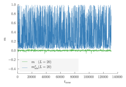
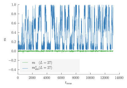
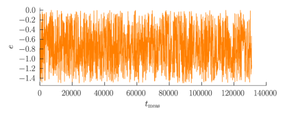
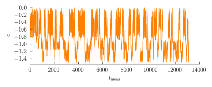
Figure 1: (a) Example time series of the multicanonical simulations for an intermediate lattice with linear size $L=20$. The upper row shows the normalized magnetization $m$ and the fuki-nuke observable $m_{\rm abs}^{x}$, the lower row shows the energy per system volume $e=E/L^{3}$. (b) The same for a large lattice with linear size $L=27$.

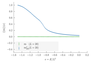
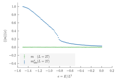
Figure 2: Microcanonical estimators for the magnetization $m$ and fuki-nuke parameter $m_{\rm abs}^{x}$ for lattices with size $L=20$ and $L=27$, where we used $100$ bins for the energy $e$ in this representation. Statistical errors are obtained from Jackknife error analysis with $20$ blocks.

In Fig. 1 we show the full time series for the magnetization $m$ and the fuki-nuke parameter $m^{x}_{\rm abs}$ of the multicanonical measurements for an intermediate ($L=20$) and the largest ($L=27$) lattice size in the simulations along with the system energy. The time series of the energy per system volume $e=E/L^{3}$ of the larger lattice can be seen to be reflected numerous times at $e\simeq-0.9$ (coming from the disordered phase) and $e\simeq-1.2$ (coming from the ordered phase) which shows qualitatively that additional, athermal and non-trivial barriers may be apparent in the system [14]. It is clear that the standard magnetization is not a suitable order parameter, since it continues to fluctuate around zero even though the system transits many times between ordered and disordered phases in the course of the simulation. The fuki-nuke order parameter, on the other hand, shows a clear signal for the transition, tracking the jumps which are visible in the energy time series. This is also reflected in Fig. 2, where we show the estimators of the microcanonical expectation values $\langle\langle\cdot\rangle\rangle$ of our observables $O$,

$$\langle\langle O\rangle\rangle(E)=\sum\limits_{O}O\,\Omega(E,O)\Big{/}\sum\limits_{O}\Omega(E,O)\;,$$ (17)

where the quantity $\Omega(E,O)$ is the number of states with energy $E$ and value $O$ of any of the observables, in this case either the magnetization $m$ or one of the fuki-nuke parameters. We get an estimator for $\Omega(E,O)$ by counting the occurrences of the pairs $(E,O)$ in the time series and weighting them with $W^{-1}(E)$. For clarity in the graphical representation in Figs. 2 and 3 we only used a partition of $100$ bins for the energy interval. An estimate for the statistical error of each bin is calculated by Jackknife error analysis [15], decomposing the time series into $N_{\rm B}=20$ non-overlapping blocks of length $b=N/N_{\rm B}$. The $i$-th Jackknife estimator is given by

$$\langle\langle O\rangle\rangle^{i}(E)=\sum\limits_{O}O\,\Omega^{i}(E,O)\Big{/}\sum\limits_{O}\Omega^{i}(E,O)\;,$$ (18)

with $\Omega^{i}$ being the occurrences of pairs $(E,O)$ in a reduced time series where the $i$-th block of length $b$ has been omitted. The variance of the Jackknife estimators then is proportional to the squared statistical error of their mean $\langle\overline{\langle O\rangle\rangle^{i}(E})=(1/N_{\rm B})\sum_{i=1}^{N_{\rm B}}\langle\langle O\rangle\rangle^{i}(E)\approx\langle\langle O\rangle\rangle(E)$,

$$\varepsilon^{2}_{\langle\overline{\langle O\rangle\rangle^{i}(E})}=\frac{N_{\rm B}-1}{N_{\rm B}}\sum\limits_{i=1}^{N_{\rm B}}\left(\langle\langle O\rangle\rangle^{i}(E)-\langle\overline{\langle O\rangle\rangle^{i}(E})\right)^{2}\;,$$ (19)

where the prefactor $(N_{\rm B}-1)/N_{\rm B}$ accounts for the trivial correlations caused by reusing each data point in $N_{\rm B}-1$ estimators [15]. Aside from reducing a systematic bias in derived quantities, the Jackknife error automatically takes care of temporal correlations as long as the block length $b$ is greater than the autocorrelation time which was measured and discussed in great detail in [2]. We additionally confirmed that $N_{\rm B}=10$ and $N_{\rm B}=40$ for selected lattice sizes yield the same magnitude for the statistical error.

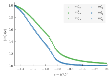
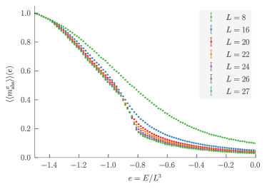
Figure 3: (a) Microcanonical estimators for the different orientations of the fuki-nuke parameters $m^{x,y,z}_{\rm abs,sq}$ for a lattice with linear size $L=20$, which fall onto two curves. The statistical errors are smaller than the data symbols and have been omitted for clarity. (b) Microcanonical estimators for the fuki-nuke parameter $m^{x}_{\rm abs}$ for several lattice sizes.

That the fuki-nuke parameters are, indeed, capable of distinguishing ordered and disordered states is depicted in Figs. 1 and 2. In the microcanonical picture we can clearly see that the different orientations of the fuki-nuke parameters are equal for the isotropic gonihedric Ising model, which we show for $L=20$ in Fig. 3(a). This confirms that the sampling is at least consistent in the simulation. We also collect the microcanonical estimators for $m^{x}_{\rm abs}$ for several lattice sizes in Fig. 3(b), where a region of approximately linear increase between $e\simeq-0.9$ and $e\simeq-1.3$ can be seen for the larger lattices. This interval corresponds to the energies of the transitional, unlikely states between the ordered and disordered phases. Plaquettes successively become satisfied towards the ordered phase and thus the estimators that measure intra- and inter-planar correlations must increase, too.

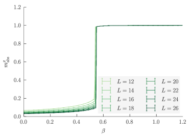
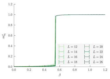
Figure 4: Canonical curves for the fuki-nuke parameters $m^{x}_{\rm abs}$ and $m^{x}_{\rm sq}$ over a broad range of inverse temperature $\beta$ for several lattice sizes $L$ (compare with the canonical data in [3]).

As we stored the full time series along with its weight function, we are able to measure the microcanonical estimators for arbitrary functions of the measured observables $f(O)$,

$$\langle\langle f(O)\rangle\rangle(E)=\sum\limits_{O}f(O)\,\Omega(E,O)\Big{/}\sum\limits_{O}\Omega(E,O)\;,$$ (20)

which can be exploited to give a convenient way of calculating higher-order moments as well. For canonical simulations reweighting techniques [12] allow the inference of system properties in a narrow range around the simulation temperature. That range and the accuracy are then determined by the available statistics of the typical configurations for the temperature of interest. Since multicanonical simulations yield histograms with statistics covering a broad range of energies, which is their most appealing feature and common to flat-histogram techniques, it is possible to reweight to a broad range of temperatures. The canonical estimator at finite inverse temperature $\beta>0$ is thus obtained by

$$\langle O\rangle(\beta)=\sum\limits_{E}\langle\langle O\rangle\rangle(E)\,e^{-\beta E}\Big{/}\sum\limits_{E}e^{-\beta E}\;,$$ (21)

and again Jackknife error analysis is employed for an estimate of the statistical error, where we form individual Jackknife estimators by inserting the $i$-th microcanonical estimator of Eq. (18) into Eq. (21) and apply an analogue to Eq. (19).

Since the microcanonical estimators for different orientations agree within error bars the canonical values will also be the same. Therefore, in Fig. 4 we only show one orientation for the two different fuki-nuke parameters. The overall behaviour of $m^{x}_{\rm abs}$ and $m^{x}_{\rm sq}$ from the Metropolis simulations of Ref. [3] is recaptured by the multicanonical data here. Namely, sharp jumps are found near the inverse transition temperature, as expected for an order parameter at a first-order phase transition. The transition temperature that was determined in the earlier simulations where energetic observables were measured under different boundary conditions and from a duality relation was $\beta=0.551\,334(8)$ [2]. The positions of the jumps seen here (and in the earlier simulations) depend on the lattice size, and finite-size scaling can be applied to estimate the transition temperature under the assumption that the fuki-nuke parameters are indeed suitable order parameters.

To carry out such a finite-size scaling analysis, it is advantageous to look at the canonical curves of the susceptibilities, $\chi_{O}(\beta)=\beta L^{3}\left(\langle O^{2}\rangle(\beta)-\langle O\rangle(\beta)^{2}\right)$, since their peak positions provide an accurate measure of the finite-lattice inverse transition temperature $\beta^{\chi_{O}}(L)$. As an example Fig. 5 shows the peaks of the susceptibilities belonging to $m_{\rm abs}^{x}$ and $m_{\rm sq}^{x}$ for several lattice sizes. Qualitatively the behaviour of both susceptibilities is similar and as for the specific heat [2, 16] their maxima scale proportional to the system volume $L^{3}$ but they differ in their magnitudes.

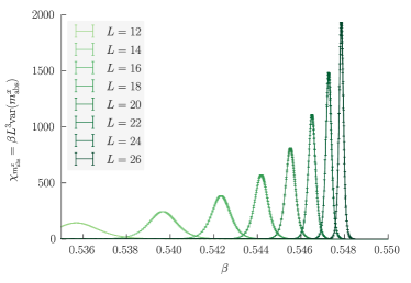
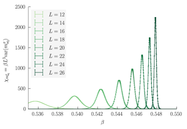
Figure 5: Canonical curves for the susceptibilities of fuki-nuke parameters $m^{x}_{\rm abs}$ and $m^{x}_{\rm sq}$ near the phase transition temperature for different lattice sizes.

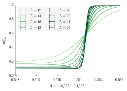
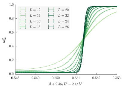
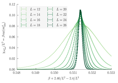
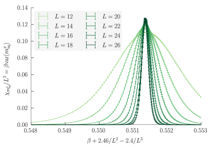
Figure 6: Canonical curves for the fuki-nuke parameters $m^{x}_{\rm abs}$ and $m^{x}_{\rm sq}$ (upper row) along with their respective susceptibilities $\chi$ normalized by the system volume (lower row) over shifted inverse temperature $\beta$ for several lattice sizes $L$.

Empirically, the peak locations for the different lattice sizes $L$ can be fitted according to the modified first-order scaling laws appropriate for macroscopically degenerate systems discussed in detail in [1, 2],

$$\beta^{\chi}(L)=\beta^{\infty}+a/L^{2}+b/L^{3}\;,$$ (22)

with free parameters $a,b$ for the available $24$ lattice sizes. Smaller lattices are systematically omitted until a fit with quality-of-fit parameter $Q$ bigger than $0.5$ is found. This gives for the estimate of the inverse critical temperature $\beta^{\chi}(L)$ from the fuki-nuke susceptibility $\chi_{m_{\rm abs}^{x}}$

$$\beta^{\chi_{m_{\rm abs}^{x}}}(L)=0.551\,37(3)-2.46(3)/L^{2}+2.4(3)/L^{3}\;,$$ (23)

with a goodness-of-fit parameter $Q=0.64$ and $12$ degrees of freedom left. Fits to the other directions $m_{\rm abs}^{y,z}$ and fits to the peak location of the susceptibilities of $m_{\rm sq}^{x,y,z}$ give the same parameters within error bars and are of comparable quality. The estimate of the phase transition temperature obtained here from the finite-size scaling of the fuki-nuke order parameter(s), $\beta^{\infty}=0.551\,37(3)$, is thus in good agreement with the earlier estimate $\beta^{\infty}=0.551\,334(8)$ reported in [2] using fits to the peak location of Binder’s energy cumulant, the specific heat and the value of $\beta$ where the energy probability density has two peaks of the same height or same weight. Interestingly, we find that the value of the coefficient for the leading correction also coincides. Assuming that the coefficient $a=-2.46(3)$ of the leading correction is related to the inverse latent heat by $a=-3\ln(2)/\Delta\hat{e}$, as with the previous estimates [2], we find from Eq. (23) that $\Delta\hat{e}=0.845(8)$, in good agreement with the latent heat $\Delta\hat{e}=0.850\,968(18)$ reported earlier in [2]. For visual confirmation of the finite-size scaling, the fuki-nuke magnetizations $m^{x}_{\rm abs,sq}$ along with their susceptibilities divided by the system volume are plotted in Fig. 6 by shifting the $x$-axis according to the scaling law, incorporating the fit parameters. The peak locations of the susceptibilities then all fall on the inverse transition temperature.

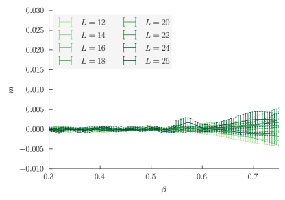
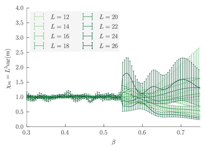
Figure 7: Canonical curves for the magnetization $m$ and the susceptibility $\chi_{m}$ over a broad range of inverse temperatures $\beta$ for several lattice sizes $L$.

In the earlier work [3] the susceptibility $\chi_{m}$ of the standard magnetization $m$ unexpectedly behaved like an order parameter and it continues to behave idiosyncratically in the multicanonical simulations, but in a different manner. For compatibility with [3], the magnetic susceptibility divided by the inverse temperature, $\chi_{m}=L^{3}(\langle m^{2}\rangle-\langle m\rangle^{2})$, is plotted in Fig. 7 along with the standard magnetization on a very small vertical scale (note that $m$ should be between $-1$ and $+1$). $\chi_{m}=1$ in the high-temperature phase but for the ordered, low-temperature phase the error rapidly increases below the transition temperature, though it is clear that the susceptibility is non-zero in this case too. Since $\langle m\rangle=0$, the behaviour of $\langle m^{2}\rangle$ can provide insight into this behaviour of the susceptibility. Above the transition temperature in the high-temperature phase the sum over the free spin variables behaves like a random walk with unit step-size, therefore the expectation value of the squared total magnetization is given by $\langle M^{2}\rangle=L^{3}$. Taking the normalization $m=M/L^{3}$ into account gives $\chi_{m}=1$ in this region, as seen in Fig. 7.

Below the transition temperature, it is plausible that simulations in general get trapped in the vicinity of one of the degenerate low-temperature phases, each of which will have a different magnetization. A canonical simulation cannot overcome the huge barriers in the system and “freezes” with the same magnetization that the system had when entering the ordered phase. This accounts for the zero variance seen in the Metropolis simulations of [3] below the transition temperature, since $\left<m\right>$ is frozen. In multicanonical simulations, on the other hand, the system travels between ordered and disordered phases, thus picking one of the possible magnetizations each time it transits to an ordered phase which it sticks with until it decorrelates again in the disordered phase. Therefore, what is seen in the low-temperature region of Fig. 7 for $\chi_{m}$ is that the variance of $m$ is taking on rather arbitrary values due to the low statistics obtained compared to the large number, $q=2^{3L}$, of degenerate phases one would have to visit to sample $\langle m^{2}\rangle$ properly. Even with multicanonical simulations it is not possible to visit all of these macroscopically degenerate phases, and the increasing error bars reflects this. In the canonical case one gets stuck with one magnetization and would not notice the different values, leading to much more severe ergodicity problems in the finite simulation runs.

We investigate further the behaviour of the standard magnetization and susceptibility and fuki-nuke magnetizations in the model by preparing several fixed configurations with a given magnetization for a lattice with $10^{3}$ spins and then only flipping complete planes of spins (a “flip-only” update), measuring the running average of the magnetization and fuki-nuke parameters. An example with the first thousand out of a total of $10^{6}$ measurements is shown in Fig. 8 for three configurations picked at random from the ordered ($e=-1.46$), intermediate ($e=-1.29$) and disordered ($e=-0.80$) regions, respectively, along with the histograms for the magnetization in Fig. 9 obtained using the non-local flip-only update. It can be seen that whatever the initial value the running average of the (standard) magnetization becomes zero if one takes a long enough run so, as expected, the flip symmetry precludes a non-zero value. The fuki-nuke order parameters, on the other hand, should be invariant with respect to the plane-flip symmetry and this is clearly the case in Fig. 8(a), where the values of $m_{\rm abs}^{x}$ remain constant for the ordered, intermediate and disordered starting configurations.

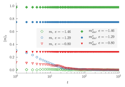
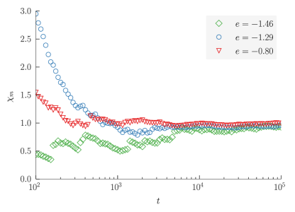
Figure 8: (a) Running average of the standard magnetization $m$ and fuki-nuke parameter $m_{\rm abs}^{x}$ plotted against the number $t$ of plane-flips for three random realizations of the ordered ($e=-1.46$), intermediate ($e=-1.29$) and disordered ($e=-0.80$) configurations of a lattice with linear size $L=10$. (b) Running average of the standard magnetic susceptibility $\chi_{m}$ plotted against the number $t$ of plane-flips for the same three realizations. Note that the $t$-axis starts at $10^{2}$ because $\chi_{m}$, being a variance, needs sufficiently many measurements to be meaningful.

The running average of the standard magnetic susceptibility $\chi_{m}$ is plotted in a similar fashion in Fig. 8(b), where it can be seen that the ordered, intermediate and disordered configurations all converge after initial transients to values of $\chi_{m}$ close to 1. The non-local plane-flips thus allow enough variability in the magnetization for the expected susceptibility value of $\chi_{m}=1$ to be at least approximately attained even in the ordered phase, unlike the case of purely local spin flips. This suggests there might be some utility in incorporating such moves into a Metropolis simulation of the plaquette model to improve the ergodicity properties.

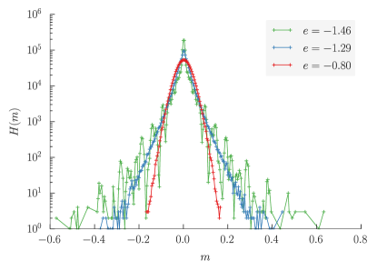
Figure 9: The histograms $H(m)$ of the standard magnetization for a total number of $10^{6}$ random plane-flips on a semi-logarithmic scale.

The histograms $H(m)$ of the magnetization shown in Fig. 9 on a semi-logarithmic scale display interesting behaviour. They are symmetric around zero for all of the starting configurations because of the $\mathbb{Z}_{2}$ symmetry of the Ising spins but they have rather different shapes in each case. The disordered starting configuration ($e=-0.80$) has a smooth maximum at $m=0$, but both the intermediate ($e=-1.29$) and ordered ($e=-1.46$) starting configurations generate sharp peaks at $m=0$. The pronounced peaks and valleys in the ordered histogram are presumably a consequence of the difficulty of reaching certain magnetization values (and the greater ease of reaching others) from an ordered starting configuration using only plane flips.

It would be interesting to construct and simulate a multimagnetic ensemble [17], where the weights give constant transition rates between configurations with different magnetizations to elucidate further on the magnetic and geometric barriers, as well as to confirm that $\langle m\rangle=0$ and $\chi=1$ for the low-temperature phase.

4 Conclusions

The multicanonical simulations presented here provide strong support for the idea that the plaquette gonihedric Ising model displays the same planar, fuki-nuke order seen in the strongly anisotropic limit of the model. In addition, the finite-size scaling analysis of the fuki-nuke order parameters gives scaling exponents in good agreement with the analysis of energetic quantities carried out in [2] and clearly displays the effect of the macroscopic low-temperature phase degeneracy on the corrections to scaling. The transition temperature obtained here from the scaling of the fuki-nuke order parameters, and the amplitude for the leading correction to scaling term were found to be the same as those extracted from energetic observables. The analysis of the magnetic order parameters carried out here is thus complementary to the analysis of energetic observables in [2] and fully consistent with it.

The peculiar behaviour of the susceptibility of the standard magnetization $\chi_{m}$ in the earlier Metropolis simulations of [3] was confirmed to be an artefact of the employed algorithm. However, even with multicanonical simulations, sampling the macroscopically degenerate low-temperature phase efficiently is difficult. Such problems could in principle be eased by introducing the plane-flips which provide a valid Monte Carlo update themselves and we investigated the behaviour of the standard magnetization and the fuki-nuke order parameters when such updates were applied.

With the work reported here on magnetic observables and the earlier multicanonical investigations of energetic quantities in [1, 2] the equilibrium properties of the $3d$ plaquette gonihedric Ising model are now under good numerical control and the order parameter has been clearly identified. In the light of this clearer understanding, it would be worthwhile re-investigating non-equilibrium properties, in particular earlier suggestions [6, 18, 19] that the model might serve as a generic example of glassy behaviour, even in the absence of quenched disorder.

References

- [1] M. Mueller, W. Janke and D. A. Johnston, Phys. Rev. Lett. 112 (2014) 200601.
- [2] M. Mueller, D. A. Johnston and W. Janke, Nucl. Phys. B 888 (2014) 214.
- [3] D. A. Johnston, J. Phys. A: Math. Theor. 45 (2012) 405001.
- [4] M. Suzuki, Phys. Rev. Lett. 28 (1972) 507.
-
[5]
Y. Hashizume and M. Suzuki, Int. J. Mod. Phys. B 25 (2011) 73;
Y. Hashizume and M. Suzuki, Int. J. Mod. Phys. B 25 (2011) 3529. - [6] C. Castelnovo, C. Chamon and D. Sherrington, Phys. Rev. B 81 (2010) 184303.
-
[7]
G. K. Savvidy and F.J. Wegner, Nucl. Phys. B 413 (1994) 605;
G. K. Savvidy and K.G. Savvidy, Phys. Lett. B 324 (1994) 72;
G. K. Savvidy and K.G. Savvidy, Phys. Lett. B 337 (1994) 333;
G. K. Bathas, E. Floratos, G. K. Savvidy and K. G. Savvidy, Mod. Phys. Lett. A 10 (1995) 2695;
G. K. Savvidy, K. G. Savvidy and F. J. Wegner, Nucl. Phys. B 443 (1995) 565;
G. K. Savvidy and K. G. Savvidy, Mod. Phys. Lett. A 11 (1996) 1379;
G. K. Savvidy, K. G. Savvidy and P. G. Savvidy, Phys. Lett. A 221 (1996) 233;
D. Johnston and R. P. K. C. Malmini, Phys. Lett. B 378 (1996) 87;
G. Koutsoumbas, G. K. Savvidy and K. G. Savvidy, Phys. Lett. B 410 (1997) 241;
J. Ambjørn, G. Koutsoumbas, G. K. Savvidy, Europhys. Lett. 46 (1999) 319;
G. Koutsoumbas and G. K. Savvidy, Mod. Phys. Lett. A 17 (2002) 751. -
[8]
R. Pietig and F. Wegner, Nucl. Phys. B 466 (1996) 513;
R. Pietig and F. Wegner, Nucl. Phys. B 525 (1998) 549. - [9] A. Lipowski, J. Phys. A 30 (1997) 7365.
-
[10]
B. A. Berg and T. Neuhaus, Phys. Lett. B 267 (1991) 249;
B. A. Berg and T. Neuhaus, Phys. Rev. Lett. 68 (1992) 9. - [11] W. Janke, Int. J. Mod. Phys. C 03 (1992) 1137.
-
[12]
A. M. Ferrenberg and R. H. Swendsen, Phys. Rev. Lett. 61 (1988) 2635;
W. Janke, in Computational Physics: Selected Methods – Simple Exercises – Serious Applications, eds. K. H. Hoffmann and M. Schreiber (Springer, Berlin, 1996), p. 10. -
[13]
W. Janke, Physica A 254 (1998) 164;
W. Janke, in Computer Simulations of Surfaces and Interfaces, eds. B. Dünweg, D. P. Landau, and A. I. Milchev, NATO Science Series, II. Math. Phys. Chem. 114 (Kluwer, Dordrecht, 2003), p. 137. - [14] A. Nußbaumer, E. Bittner and W. Janke, Phys. Rev. E 77 (2008) 041109.
-
[15]
B. Efron,
The Jackknife, the Bootstrap and other Resampling Plans (Society for Industrial and Applied Mathematics, Philadelphia, 1982);
W. Janke, in Proceedings of the Euro Winter School Quantum Simulations of Complex Many-Body Systems: From Theory to Algorithms, eds. J. Grotendorst, D. Marx, and A. Muramatsu, NIC Series Vol. 10 (John von Neumann Institute for Computing, Jülich, 2002), p. 423;
M. Weigel and W. Janke, Phys. Rev. Lett. 102 (2009) 100601;
M. Weigel and W. Janke, Phys. Rev. E 81 (2010) 066701. - [16] M. Mueller, W. Janke and D. A. Johnston, Physics Procedia 57 (2014) 68.
- [17] B. A. Berg, U. Hansmann and T. Neuhaus, Phys. Rev. B 47 (1993) 497.
-
[18]
A. Lipowski, J. Phys. A 30 (1997) 7365;
A. Lipowski and D. A. Johnston, J. Phys. A 33 (2000) 4451;
A. Lipowski and D. A. Johnston, Phys. Rev. E 61 (2000) 6375;
M. Swift, H. Bokil, R. Travasso, and A. Bray, Phys. Rev. B 62 (2000) 11494. - [19] D. A. Johnston, A. Lipowski, and R. P. K. C. Malmini, in Rugged Free Energy Landscapes: Common Computational Approaches to Spin Glasses, Structural Glasses and Biological Macromolecules, ed. W. Janke, Lecture Notes in Physics 736 (Springer, Berlin, 2008), p. 173.