Millimeter Wave MIMO Channel Tracking Systems

Abstract

We consider channel/subspace tracking systems for temporally correlated millimeter wave (e.g., E-band) multiple-input multiple-output (MIMO) channels. Our focus is given to the tracking algorithm in the non-line-of-sight (NLoS) environment, where the transmitter and the receiver are equipped with hybrid analog/digital precoder and combiner, respectively. In the absence of straightforward time-correlated channel model in the millimeter wave MIMO literature, we present a temporal MIMO channel evolution model for NLoS millimeter wave scenarios. Considering that conventional MIMO channel tracking algorithms in microwave bands are not directly applicable, we propose a new channel tracking technique based on sequentially updating the precoder and combiner. Numerical results demonstrate the superior channel tracking ability of the proposed technique over independent sounding approach in the presented channel model and the spatial channel model (SCM) adopted in 3GPP specification.

I Introduction

It is now well projected that conventional cellular systems deployed in the over-crowded sub-3 GHz frequency bands are not capable to support the recent exponentially growing data rate demand, even though advanced throughput boosting multiple-input multiple-output (MIMO) techniques are employed. Thus, there is gradual movement to shift the operating frequency of cellular systems from the microwave spectrum to millimeter wave spectrum (3 GHz to 300 GHz). The large bandwidth available in the millimeter wave spectrum makes its application for indoor [1] and even outdoor [2] transmission feasible.

However, outdoor millimeter wave channel is challenging. The millimeter wave propagation suffers from severe path loss and other environmental obstructions [3]. The small wavelength of the millimeter wave (relative to the microwave) ensures that large-sized arrays can be implemented with a small form factor. As a result, these outdoor challenges can be overcome by providing sufficient array gain using large-sized array antennas and analog beamforming and combining at the base station (BS) and the mobile station (MS) [2]. Hybrid precoding/combining, consisting of analog and digital precoders/combiners at the BS/MS, has been investigated to show close-to-optimal data rate in a cost- and energy-efficient way [4, 5, 6]. Unlike the conventional digital precoding/combining technique, the analog precoder/combiner are composed of groups of phase shifters. This is, the weights of the analog precocer/combiner have constant-modulus property, imposing hardware constraints.

Following the parametric channel model from conventional MIMO systems [7], the millimeter wave channels can be modeled using angles of arrival (AoA), angles of departure (AoD) and propagation path gains [1, 2, 4, 8]. The number of propagation paths is limited, resulting in a sparse channel, due to the directional transmission and high attenuation of millimeter waves. To facilitate the hybrid precoding/combining techniques, usable channel estimates at the MS and BS are crucial. However, estimating the channel via conventional training-based techniques is infeasible and ping-pong based indoor/outdoor channel sounding (or sampling) techniques have recently been studied in [1, 2, 4]. The channel sounding probes the channel using a set of predefined beamforming vectors, i.e., codebook, for a fixed number of channel uses, and selects the best beamformer/precoder according to certain criteria.

MIMO systems, in practice, can leverage temporal correlation between channel realizations to further enhance the system performance. The previous work in conventional MIMO spatial multiplexing systems devises various subspace tracking techniques, e.g., stochastic gradient approach [9], geodesic precoding [10], and differential feedback [11], in temporally correlated MIMO channels. These techniques adapt the precoder to the temporal channel correlation statistics and thereby, enhancing the system performance. Although the extension of these techniques to the millimeter wave MIMO systems is not straightforward, it would be possible to devise a useful channel tracking technique by modifying the previous work (e.g., [9, 10, 11]), which is our focus in this paper.

In this paper, we propose a channel tracking technique for the millimeter wave MIMO systems employing hybrid precoding/combining architecture in the temporally correlated MIMO channels. We assume a time division duplex (TDD) system exploiting channel reciprocity. The primary challenges we face here are how to tractably model the channel evolution in the millimeter wave scenario and how to devise a hybrid precoding/combining algorithm that efficiently tracks the channel evolution. In the absence of a tractable temporally correlated millimeter wave channel model, we first present, in this paper, a temporally correlated MIMO channel evolution model by modifying the parametric channel models. The proposed channel tracking algorithm is based on updating each column of the analog precoder and combiner. We call this approach the mode-by-mode update, where each mode represents one column of the analog precoder and combiner. It sequentially adapts the analog precoder and combiner to the temporal correlation statistics. The digital precoder and combiner updates follow a conventional MIMO precoder and combiner design procedure. Simulation results verify that the proposed channel tracking technique successfully tracks the channel variations in the presented temporally correlated channel model and spatial channel model (SCM) [12].

The rest of the paper is organized as follows. Section II describes the system model and presents the temporally correlated millimeter wave MIMO channel model, Section III details the proposed tracking technique, and the numerical results are presented in Section IV. Concluding remarks are given in Section V.

II System Architecture and Temporally Correlated Channel Model

In this section, we describe the system model of the millimeter wave MIMO hybrid precoding/combining systems. We then subsequently present the temporally correlated millimeter wave MIMO channel model.

II-A System Architecture

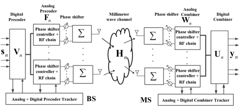
Figure 1: Block diagram of millimeter wave MIMO hybrid precoding/combining and channel tracking system.

Assuming a narrowband block-fading channel model and $N_{s}$ data streams, the output signal ${\mathbf{y}}_{n}\in{\mathbb{C}}^{N_{s}\times 1}$ in Fig. 1 at the channel block $n$ in the downlink is modeled via

$${\mathbf{y}}_{n}={\mathbf{U}}^{*}_{n}{\mathbf{W}}^{*}_{n}{\mathbf{H}}_{n}{\mathbf{F}}_{n}{\mathbf{V}}_{n}{\mathbf{s}}_{n}+{\mathbf{U}}_{n}^{*}{\mathbf{W}}_{n}^{*}{\mathbf{n}}_{n}.$$ (1)

The ${\mathbf{U}}_{n}\in{\mathbb{C}}^{N_{rf}\times N_{s}}$ and ${\mathbf{W}}_{n}\in{\mathbb{C}}^{N_{r}\times N_{rf}}$ represent the digital combiner and analog combiner at the MS, respectively, with $\|{\mathbf{W}}_{n}{\mathbf{U}}_{n}\|_{F}^{2}=N_{s}$. The $N_{r}$ and $N_{rf}$, respectively, denote the number of antennas and number of RF chains at the MS. The ${\mathbf{H}}_{n}\in{\mathbb{C}}^{N_{r}\times N_{t}}$ is the millimeter wave channel from the BS to MS, where $N_{t}$ denotes the number of BS antennas. We assume for simplicity that both BS and MS have the same number of RF chains. The ${\mathbf{V}}_{n}\in{\mathbb{C}}^{N_{rf}\times N_{s}}$ and ${\mathbf{F}}_{n}\in{\mathbb{C}}^{N_{t}\times N_{rf}}$ represent the digital precoder and analog precoder at the BS, respectively, with $\|{\mathbf{F}}_{n}{\mathbf{V}}_{n}\|_{F}^{2}=N_{s}$. The ${\mathbf{s}}_{n}\in{\mathbb{C}}^{N_{s}\times 1}$ in (1) is the data symbol vector transmitted from the BS, constrained to have $E[{\mathbf{s}}_{n}{\mathbf{s}}_{n}^{*}]=\frac{1}{N_{s}}{\mathbf{I}}_{N_{s}}$, and ${\mathbf{n}}_{n}\in{\mathbb{C}}^{N_{r}\times 1}$ is the additive Gaussian noise distributed as $\mathcal{CN}(\mathbf{0},\sigma^{2}{\mathbf{I}}_{N_{r}})$. The digital precoder ${\mathbf{V}}_{n}$ and combiner ${\mathbf{U}}_{n}$ can adjust both the phase and amplitude, while only phase control is allowed, as seen from Fig. 1, for the analog precoder ${\mathbf{F}}_{n}$ and combiner ${\mathbf{W}}_{n}$, i.e.,

$$|{\mathbf{F}}_{n}^{(i,j)}|=\frac{1}{\sqrt{N_{t}}},\,\text{and}\;|{\mathbf{W}}_{n}^{(i,j)}|=\frac{1}{\sqrt{N_{r}}}\ ,\forall i,j.$$ (2)

We assume that the phase of each element in ${\mathbf{F}}_{n}$ and ${\mathbf{W}}_{n}$ is quantized to $Q$ bits, i.e., $\angle{\mathbf{F}}_{n}^{(i,j)},\,\angle{\mathbf{W}}_{n}^{(i,j)}~{}\in\{0,2\pi(\frac{1}{2^{Q}}),\cdots,2\pi(\frac{2^{Q}-1}{2^{Q}})\}$. In general, we make an assumption that $N_{s}\leq N_{rf}\leq\min(N_{t},N_{r})$.

II-B Temporally correlated Millimeter Wave MIMO Channel Model

Based on the parametric channel model, the millimeter wave MIMO channel can be reasonably modeled by manipulating the AoAs, AoDs, and a limited number of propagation path gains, e.g., [1, 2, 4, 8]. We assume NLoS scenario [4], where the propagation path gains are modeled as independent and identically distributed (i.i.d.) Gaussian random variables,

$${\mathbf{H}}_{n}=\sqrt{\frac{N_{t}N_{r}}{L}}{\mathbf{A}}_{r}(\boldsymbol{\theta}_{n}){\mathbf{D}}_{n}{\mathbf{A}}_{t}^{*}(\boldsymbol{\phi}_{n}),$$ (3)

where ${\mathbf{D}}_{n}=\text{diag}([\alpha_{n,1},\alpha_{n,L},\cdots,\alpha_{n,L}]^{T})\in{\mathbb{C}}^{L\times L}$ is the propagation path gain matrix. The $\alpha_{n,i}$ denotes the gain of $i$th path with $\alpha_{n,i}\sim\mathcal{CN}(0,1)$ for $i=1,\cdots,L$, where $L$ is the number of propagation paths. The $\boldsymbol{\phi}_{n}=[\phi_{n,1},\phi_{n,2},\cdots,\phi_{n,L}]^{T}\in{\mathbb{R}}^{L\times 1}$ and $\boldsymbol{\theta}_{n}=[\theta_{n,1},\theta_{n,2},\cdots,\theta_{n,L}]^{T}\in{\mathbb{R}}^{L\times 1}$ in (3) denote the AoDs and AoAs of $L$ independent paths. We assume $\theta_{n,i},\phi_{n,i}\sim\mathcal{U}(-\pi,\pi),\;\forall n,i$. The ${\mathbf{A}}_{t}(\boldsymbol{\phi}_{n})\in{\mathbb{C}}^{N_{t}\times L}$ and ${\mathbf{A}}_{r}(\boldsymbol{\theta}_{n})\in{\mathbb{C}}^{N_{r}\times L}$ in (3), respectively, represent array response matrices at the BS and MS,

$${\mathbf{A}}_{t}(\boldsymbol{\phi}_{n})=\frac{1}{\sqrt{N_{t}}}[{\mathbf{a}}_{t}(\phi_{n,1}),{\mathbf{a}}_{t}(\phi_{n,2}),\cdots,{\mathbf{a}}_{t}(\phi_{n,L})]$$ (4)

and

$${\mathbf{A}}_{r}(\boldsymbol{\theta}_{n})=\frac{1}{\sqrt{N_{r}}}[{\mathbf{a}}_{r}(\theta_{n,1}),{\mathbf{a}}_{r}(\theta_{n,2}),\cdots,{\mathbf{a}}_{r}(\theta_{n,L})].$$ (5)

With uniform linear array (ULA) assumption, the ${\mathbf{a}}_{t}(\phi_{n,l})$ in (4) and ${\mathbf{a}}_{r}(\theta_{n,l})$ in (5) are given by

$${\mathbf{a}}_{t}(\phi_{n,l})=[1,e^{j\frac{2\pi}{\lambda}d\sin(\phi_{n,l})},\cdots,e^{j(N_{t}-1)\frac{2\pi}{\lambda}d\sin(\phi_{n,l})}]^{T}$$ (6)

and

$${\mathbf{a}}_{r}(\theta_{n,l})=[1,e^{j\frac{2\pi}{\lambda}d\sin(\theta_{n,l})},\cdots,e^{j(N_{r}-1)\frac{2\pi}{\lambda}d\sin(\theta_{n,l})}]^{T},$$ (7)

where $\lambda$ is the wavelength and $d$ is the inter-antenna spacing.

Based on the channel model in (3), we now present a temporal channel evolution model. The evolution of ${\mathbf{H}}_{n}$ from $n$th channel block to $(n+1)$th channel block follows

$${\mathbf{H}}_{n+1}=\sqrt{\frac{N_{t}N_{r}}{L}}{\mathbf{A}}_{r}(\boldsymbol{\theta}_{n+1}){\mathbf{D}}_{n+1}{\mathbf{A}}_{t}^{*}(\boldsymbol{\phi}_{n+1}),$$ (8)

where

$${\mathbf{D}}_{n+1}=\rho{\mathbf{D}}_{n}+\sqrt{1-\rho^{2}}{\mathbf{B}}_{n+1},$$ (9)

$${\mathbf{A}}_{r}(\boldsymbol{\theta}_{n+1})={\mathbf{A}}_{r}(\boldsymbol{\theta}_{n}+\Delta\boldsymbol{\theta}_{n}),$$ (10)

$${\mathbf{A}}_{t}(\boldsymbol{\phi}_{n+1})={\mathbf{A}}_{t}(\boldsymbol{\phi}_{n}+\Delta\boldsymbol{\phi}_{n}).$$ (11)

The $\rho=E[\alpha_{n,i}\alpha^{*}_{n+1,i}]\in[0\;1]$, $i=1,\ldots,L$, is the time correlation coefficient, which follows Jakes’ model [13] according to $\rho=J_{0}(2\pi f_{D}T)$. The $J_{0}(\cdot)$ is the zeroth order Bessel function of first kind, and the $f_{D}$ and $T$ denote the maximum Doppler frequency and channel block length, respectively. The $f_{D}=f_{c}v/c$, where $f_{c}$, $v$, and $c$ represent the carrier frequency (Hz), the speed of the MS (km/h), and $c=3\times 10^{8}$ (m/s), respectively. The ${\mathbf{B}}_{n+1}$ in (9) is the diagonal matrix with diagonal entries drawn from $\mathcal{CN}(0,1)$ and independent from ${\mathbf{D}}_{n}$. As shown in (9), the evolution of the propagation path gains is modeled as the first order Gauss-Markov process. We assume that angle variations $\Delta\boldsymbol{\theta}_{n},\Delta\boldsymbol{\phi}_{n}\sim\mathcal{U}(-\delta,\delta)$, where $\delta$ is small.

III Subspace Tracking: Algorithm Development

In this section, we detail the proposed subspace tracking technique, consisting of tracking each mode of the analog precoder and combiner one at a time (by generating a controlled perturbation around the previous mode), then followed by the digital precoder and combiner update. The motivation of the mode-by-mode update lies in that we can sound $N_{rf}$ codewords per channel use by taking the advantage of the hybrid architecture [4]. Therefore, the sounding overhead could be significantly reduced. As shown in Fig. 2, the channel block duration $T$ is decomposed into $6$ phases - the focus of this work is on the first $4$ phases.

This section only focuses on the downlink sounding used to update the analog combiner (Sec III-A), and downlink channel estimation phase used to update the digital combiner (Sec III-B). The exactly same reasoning applies for updating the analog and digital precoders as well, and will thus be omitted, for simplicity and conciseness.

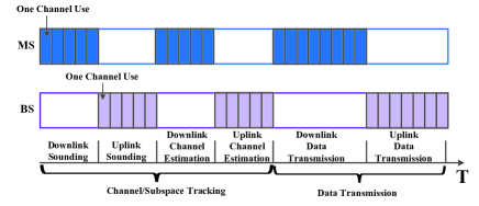
Figure 2: The graphical description of the proposed channel/subspace tracking technique.

We summarize the main steps of the algorithm. For each mode, we construct a codebook by rotating the previous mode using a group of rotation matrices [14, 11], and then we select the best codeword that maximizes the received power. After the analog combiner and precoder design, the digital precoder and combiner follow using pilot-aided conventional channel estimation of the effective channel.

III-A Downlink Sounding and Analog Combiner Update

The downlink sounding is exploited to update the analog combiner by utilizing the knowledge of previous analog combiner and time correlation statistics. Thus, given the analog combiner at instant $n$, ${\mathbf{W}}_{n}$, our aim is to leverage the correlation coefficient $\rho$ to compute the update for ${\mathbf{W}}_{n}$, i.e., ${\mathbf{W}}_{n+1}$, done in a mode-by-mode fashion.

Given that each mode is unit-modulus (i.e., (2)) and that adjacent channel blocks are temporally correlated, it is highly likely that ${\mathbf{W}}_{n}$ and ${\mathbf{W}}_{n+1}$ are relatively “close”. Thus, we first construct a rotation codebook, $\mathcal{C}=\{{\mathbf{C}}_{1},\cdots,{\mathbf{C}}_{N}\}$, ${\mathbf{C}}_{i}\in{\mathbb{C}}^{N_{r}\times N_{r}}$, ${\mathbf{C}}_{i}^{*}{\mathbf{C}}_{i}={\mathbf{C}}_{i}{\mathbf{C}}_{i}^{*}={\mathbf{I}}_{N_{r}}$, for $i=1,\cdots,N$. By applying each element in $\mathcal{C}$ to ${\mathbf{W}}_{n}^{(l)}$, i.e., ${\mathbf{C}}_{k}{\mathbf{W}}_{n}^{(l)},\ k=1,\cdots,N$, we can generate codewords for the update of ${\mathbf{W}}_{n+1}^{(l)}$, which are “close” to ${\mathbf{W}}_{n}^{(l)}$. This set of codewords for the update of $l$th mode can be collected as a matrix,

$$\widehat{{\mathbf{W}}}_{n+1,l}=[{\mathbf{C}}_{1}{\mathbf{W}}_{n}^{(l)},\cdots,{\mathbf{C}}_{N}{\mathbf{W}}_{n}^{(l)}],\ l=1,\cdots,N_{rf},$$ (12)

where the construction/selection of ${\mathbf{C}}_{1},\cdots,{\mathbf{C}}_{N}$ is investigated in Sec III-C. This latter $\widehat{{\mathbf{W}}}_{n+1,l}$ is applied to the received signal at the MS antenna to yield

$${\mathbf{x}}_{n+1,l}=\widehat{{\mathbf{W}}}_{n+1,l}^{*}{\mathbf{H}}_{n+1}{\mathbf{F}}_{n}{\mathbf{V}}_{n}\overline{{\mathbf{s}}}+\widehat{{\mathbf{W}}}_{n+1,l}^{*}{\mathbf{n}}_{n+1},$$ (13)

where ${\mathbf{F}}_{n}$ and ${\mathbf{V}}_{n}$ are the analog and digital precoder at channel block $n$, respectively, and $\overline{{\mathbf{s}}}$ is the training vector, e.g., all-ones. Given ${\mathbf{x}}_{n+1,l}$, the index of the optimal codeword is given by

$$k_{l}^{\star}=\mathop{\operatorname*{argmax}\limits}_{1\leq k\leq N}(|\mathbf{x}_{n+1,l}(k)|^{2}),$$ (14)

where ${\mathbf{x}}_{n+1,l}(k)$ denotes the $k$th element of ${\mathbf{x}}_{n+1,l}$. Note that the total number of soundings for each mode is $\lceil\frac{N}{N_{rf}}\rceil$. From (14), the ${\mathbf{W}}_{n+1}^{(l)}$ is determined by the $k_{l}^{\star}$th column of $\widehat{{\mathbf{W}}}_{n+1,l}$.

The generation of candidate vectors for the second to last mode update is slightly different from that of the first mode update. For the second to last mode, the additional step of subtracting the effect of the previously updated modes, is needed. This can be done by employing orthogonal subspace projection,

$$\widehat{{\mathbf{W}}}_{n+1,l}=({\mathbf{I}}_{N_{r}}-\boldsymbol{\Theta}(\boldsymbol{\Theta}^{*}\boldsymbol{\Theta})^{-1}\boldsymbol{\Theta}^{*})\widehat{{\mathbf{W}}}_{n+1,l},\;l\geq 2,$$ (15)

where

$$\boldsymbol{\Theta}=[{\mathbf{W}}_{n+1}^{(1)},\cdots,{\mathbf{W}}_{n+1}^{(l-1)}]\in{\mathbb{C}}^{N_{r}\times(l-1)}.$$ (16)

As the codebook $\widehat{{\mathbf{W}}}_{n+1,l}$ for $l=1,\cdots,N_{rf}$ does not guarantee hardware constraint, one possible approach is to construct an overcomplete matrix ${\mathbf{A}}_{\text{can}}\in{\mathbb{C}}^{N_{r}\times N_{\text{can}}}$, $N_{\text{can}}\gg N_{r}$, with each column vector in the form of array response vector, i.e., ${\mathbf{A}}_{\text{can}}=[{\mathbf{a}}_{r}(\varphi_{1}),\cdots,{\mathbf{a}}_{r}(\varphi_{N_{\text{can}}})]$, where $\varphi_{i}=-\pi+\frac{(2i+1)\pi}{N_{\text{can}}}\;\text{for}\;i=0,\cdots,N_{\text{can}}-1$, and replace each column vector of $\widehat{{\mathbf{W}}}_{n+1,l}$ with one from ${\mathbf{A}}_{\text{can}}$ with the closest distance. Note that the phases of the entries in ${\mathbf{A}}_{\text{can}}$ are also quantized using $Q$ bits. The replacement of the $m$th column vector of $\widehat{{\mathbf{W}}}_{n+1,l}$ can be accomplished by

$$m_{l}^{\star}=\mathop{\mathop{\mathrm{argmin}}}\limits_{1\leq j\leq N_{\text{can}}}\sqrt{1-|\widehat{{\mathbf{W}}}_{n+1,l}^{(m)^{*}}{\mathbf{A}}_{\text{can}}^{(j)}|^{2}}$$ (17)

and

$$\widehat{{\mathbf{W}}}_{n+1,l}^{(m)}={\mathbf{A}}_{\text{can}}^{(m_{l}^{\star})}.$$ (18)

As a result, the matrix $\widehat{{\mathbf{W}}}_{n+1,l}$ in (18) produces nearly orthogonal columns to the previously updated modes, making ${\mathbf{W}}_{n+1}$ approximate unitary matrix.

The selection of the optimal column for ${\mathbf{W}}_{n+1}^{(l)}$ for $l\geq 2$ follows the procedures in (13) and (14). The above process is repeated for a number $T_{\text{max}}$ of channel blocks (summarized in Algorithm 1).

Algorithm 1 Analog Combiner Update

1:Initial Values: ${\mathbf{W}}_{0}$, ${\mathbf{F}}_{0}$, ${\mathbf{V}}_{0}$, ${\mathbf{U}}_{0}$, $\rho$, ${\mathbf{A}}_{\text{can}}$, $\mathcal{C}=\{{\mathbf{C}}_{1},\cdots,{\mathbf{C}}_{N}\}$.

2:for $n=0,\cdots,T_{\text{max}}$ do

3:     for $l=1,\cdots,N_{rf}$ do

4:         $\widehat{{\mathbf{W}}}_{n+1,l}=[{\mathbf{C}}_{1}{\mathbf{W}}_{n}^{(l)},\cdots,{\mathbf{C}}_{N}{\mathbf{W}}_{n}^{(l)}]$;

5:         if $l\geq 2$ then

6:              $\boldsymbol{\Theta}=[{\mathbf{W}}_{n+1}^{(1)},\cdots,{\mathbf{W}}_{n+1}^{(l-1)}]$;

7:              $\widehat{{\mathbf{W}}}_{n+1,l}=({\mathbf{I}}_{N_{r}}-\boldsymbol{\Theta}(\boldsymbol{\Theta}^{*}\boldsymbol{\Theta})^{-1}\boldsymbol{\Theta}^{*})\widehat{{\mathbf{W}}}_{n+1,l}$;

8:         end if

9:         Replace each column of $\widehat{{\mathbf{W}}}_{n+1,l}$ according to (17)

10:         and (18).

11:         ${\mathbf{x}}_{n+1,l}=\widehat{{\mathbf{W}}}_{n+1,l}^{*}{\mathbf{H}}_{n+1}{\mathbf{F}}_{n}{\mathbf{V}}_{n}\overline{{\mathbf{s}}}+\widehat{{\mathbf{W}}}_{n+1,l}^{*}{\mathbf{n}}_{n+1}$;

12:         $k_{l}^{\star}=\mathop{\operatorname*{argmax}}\limits_{1\leq k\leq N}(|\mathbf{x}_{n+1,l}(k)|^{2})$;

13:         ${\mathbf{W}}_{n+1}^{(l)}=\widehat{{\mathbf{W}}}_{n+1,l}^{(k_{l}^{\star})}$;

14:     end for

15:end for

III-B Digital Channel Estimation and Combiner Update

After the analog combiner update, the digital combiner is updated during the downlink effective channel estimation (phase 3 in Fig. 2), based on well-known pilot based channel estimation schemes. The effective channel ${\mathbf{H}}_{n+1,\text{eff}}\in{\mathbb{C}}^{N_{rf}\times N_{rf}}$ can be expressed as,

$${\mathbf{H}}_{n+1,\text{eff}}={\mathbf{W}}_{n+1}^{*}{\mathbf{H}}_{n+1}{\mathbf{F}}_{n+1},$$ (19)

where ${\mathbf{F}}_{n+1}$ is the updated analog precoder during the second phase of the channel tracking technique in Fig. 2. Since characterizing the statistics of the effective channel in (19) is not tractable, we rather employ a simple least squares (LS) channel estimation technique [15] and leave any possible improvements (e.g., using Kalman tracking, particle filters, etc.) for the future work.

Assume a unitary training signal ${\mathbf{P}}\in{\mathbb{C}}^{N_{rf}\times N_{P}}$, i.e., ${\mathbf{P}}{\mathbf{P}}^{*}={\mathbf{I}}_{N_{rf}}$ with $N_{P}\geq N_{rf}$ being the channel training block length. The received signal during the training phase is

$${\mathbf{Q}}_{n+1}={\mathbf{H}}_{n+1,\text{eff}}{\mathbf{P}}+{\mathbf{Z}}_{n+1},$$ (20)

where ${\mathbf{Z}}_{n+1}\in{\mathbb{C}}^{N_{rf}\times N_{P}}$ is the additive Gaussian noise matrix with its elements i.i.d. as $\mathcal{CN}(0,\sigma^{2})$. Then, the LS channel estimate yields

$$\widehat{{\mathbf{H}}}_{n+1,\text{eff}}={\mathbf{Q}}_{n+1}{\mathbf{P}}^{*}.$$ (21)

The singular value decomposition (SVD) is applied to decompose $\widehat{{\mathbf{H}}}_{n+1,\text{eff}}=\widehat{{\mathbf{U}}}_{n+1}\widehat{\mathbf{\Lambda}}_{n+1}\widehat{{\mathbf{V}}}_{n+1}^{*}$, where $\widehat{{\mathbf{U}}}_{n+1}\in{\mathbb{C}}^{N_{rf}\times N_{rf}}$ and $\widehat{{\mathbf{V}}}_{n+1}\in{\mathbb{C}}^{N_{rf}\times N_{rf}}$ denote the left and right singular (and unitary) matrices of $\widehat{{\mathbf{H}}}_{n+1,\text{eff}}$, respectively. The $\widehat{\mathbf{\Lambda}}_{n+1}\in\mathbb{R}^{N_{rf}\times N_{rf}}$ is the diagonal matrix $\widehat{\mathbf{\Lambda}}_{n+1}=\text{diag}([\lambda_{1},\cdots,\lambda_{N_{rf}}]^{T})$ with $\lambda_{1}\geq\lambda_{2}\geq\cdots\geq\lambda_{N_{rf}}\geq 0$. Then, ${\mathbf{U}}_{n+1}=[\widehat{{\mathbf{U}}}_{n+1}]_{:,1:N_{s}}$ is selected as the digital combiner at the MS (the same applies for the digital precoder update in the uplink).

III-C Design of Rotation Codebook

This subsection concerns systematic design of the rotation codebook $\mathcal{C}$. In our approach, the generation of $\mathcal{C}$ utilizes a basis codebook $\mathcal{R}=\{{\mathbf{R}}_{1},\cdots,{\mathbf{R}}_{N}\}$. Each codeword ${\mathbf{R}}_{i}\in{\mathbb{C}}^{N_{r}\times N_{r}}$ from $\mathcal{R}$ is structured such that

$${\mathbf{R}}_{i}={\mathbf{R}}^{i}=\left(\begin{array}[]{ccc}\text{exp}(j\theta_{1})&&\textbf{0}\\ &\cdots&\\ \textbf{0}&&\text{exp}(j\theta_{N_{r}})\\ \end{array}\right)^{i},\ i=1,\cdots,N,$$ (22)

$\theta_{k}\in\{0,\cdots,\frac{2(M-1)\pi}{M}\},\ k=1,\cdots,N_{r}$, and $M$ is a positive prime number such that $M>N_{r}$. Note that given ${\mathbf{R}}$, ${\mathbf{R}}^{i}$ is diagonal, and thus is a unitary matrix (where $i\in{\mathbb{R}}$ can be any real number, but in our case, $i=1,...,N$). The basis codebook $\mathcal{R}$ can be reasonably designed by maximizing the minimum chordal distance between any two codewords in $\mathcal{R}$, i.e.,

$$\mathcal{R}=\underset{\{\widetilde{\mathcal{R}}\}}{\operatorname*{argmax}}\left(\underset{\begin{subarray}{c}1\leq i<j\leq N\\ {\mathbf{R}}_{i},{\mathbf{R}}_{j}\in\widetilde{\mathcal{R}}\end{subarray}}{\min}\sqrt{N_{r}-|\textrm{diag}({\mathbf{R}}_{i})^{*}\textrm{diag}({\mathbf{R}}_{j})|^{2}}\right).$$ (23)

Note that the latter design criterion does not adapt to the temporal correlation structure of the channel. When time correlation is presented (i.e., when modes of adjacent channel blocks are “close”), the adaptation of the rotation codebook $\mathcal{R}$ follows

$${\mathbf{G}}_{i}=\epsilon\mathbf{I}_{N_{r}}+\sqrt{1-\epsilon^{2}}{\mathbf{R}}_{i},\;\forall\;i=1,\cdots,N.$$ (24)

We model the $\epsilon$ as a linear function of $\rho$, i.e., $\epsilon=\gamma\rho$ with $0<\gamma\leq 1$. The (24) is applied to generate points (or perturbations) on a sphere centered at the point $\epsilon{\mathbf{I}}_{N_{r}}$ with radius $\sqrt{1-\epsilon^{2}}$. Since ${\mathbf{G}}_{i}$ is not a unitary matrix, we need to project ${\mathbf{G}}_{i}$ onto the unitary matrix space. The projection can easily be implemented by normalizing ${\mathbf{G}}_{i}$ such that ${\mathbf{C}}_{i}={\mathbf{G}}_{i}/\|\text{diag}({\mathbf{G}}_{i})\|_{2}$, which yields the rotation codebook $\mathcal{C}$ used to rotate the previous mode in (12).

IV Numerical Results

The Monte Carlo simulations are carried out to demonstrate the performance of the proposed tracking scheme. We evaluate the achievable throughput at channel block $n$, which can be expressed as

$$R_{n}= \log_{2}\bigg{(}\text{det}\Big{(}\mathbf{I}_{N_{s}}+\frac{1}{\sigma^{2}N_{s}}({\mathbf{U}}_{n}^{*}{\mathbf{W}}_{n}^{*}{\mathbf{W}}_{n}{\mathbf{U}}_{n})^{-1}{\mathbf{U}}_{n}^{*}{\mathbf{W}}_{n}^{*}{\mathbf{H}}_{n}$$

$${\mathbf{F}}_{n}{\mathbf{V}}_{n}{\mathbf{V}}_{n}^{*}{\mathbf{F}}_{n}^{*}{\mathbf{H}}_{n}^{*}{\mathbf{W}}_{n}{\mathbf{U}}_{n}\Big{)}\bigg{)}.$$ (25)

We set $N_{t}=N_{r}=64$ with $N_{rf}=4$, i.e., $4$ RF chains, $d=\frac{\lambda}{2}$, and $L=4$.

We adopt the SCM [12] to emulate a close-to-real millimeter wave propagation environment. For the SCM channel emulation, we choose the ‘urban micro’ environment. In order to satisfy the sparsity property of the millimeter wave MIMO channel, the number of paths is set to $4$, and the number of subpaths per path is also set to $4$. We set the powers of the $4$ paths to $[0.8893\;0.0953\;0.0107\;0.0047]$. Note that the default value of subpaths per path in [12] is $20$, so we just pick the first $4$ subpaths in our case. The inter-antenna spacing is also set to $\frac{\lambda}{2}$ at both the BS and MS. We assume the system is deployed in E-band and set the carrier frequency to $72$ GHz. For the evaluation, as shown in Fig. 3, several values of velocity for the MS are considered (e.g., $v=1.0,3.0,4.4$ km/h). Notice that we can not set the $\rho$ parameter in SCM. We keep the default values of SCM for the remaining parameters.

The maximum number of channel blocks $T_{\text{max}}$ is set to $10$ in our simulation. The number of training sequences for the digital combiner update is $N_{P}=1.5N_{rf}$, and the SNR (i.e., $1/\sigma^{2}$) is set to $0$ dB. The ${\mathbf{A}}_{\text{can}}$ is with the form of array response matrix (e.g., (4) and (5)) with 200 columns, i.e., $N_{\text{can}}=200$. The $Q=4$ bits are used to quantize the phases of analog combiner and precoder. We assume that the $\delta$ for angle variations in Section II increases linearly with $v$, $\delta=3.0^{\circ},9.0^{\circ},13.2^{\circ}$, corresponding to the aforementioned $v$ values. For $v=3$ km/h and $f_{c}=72$ GHz, the maximum Doppler frequency is $f_{D}=200$ Hz and the coherence time is roughly $T_{c}=5$ ms. If we define the channel block length as $10\%$ (with sufficient coherency) of $T_{c}$, then the latter is $0.5$ ms: this value, along with calculated maximum Doppler frequency, result in the temporal correlation coefficient being $\rho=0.9037$, according to Jakes’ model [13]. We fix the channel block length to be $0.5$ ms for the computation of the $\rho$ values and associated velocities. We further assume the system employs the OFDM technique accommodating a broad bandwidth of $1$ GHz with oversampling factor $1.1$. Then, provided $1024$ FFT size, one OFDM symbol duration is $\frac{1024}{1.1\ GHz}\approx 1\ us$, implying the system can resort to around $500$ channel uses during one channel block. Those values will allow the computation of the total overhead (sounding overhead plus training overhead) shortly.

The benchmark scheme (also called independent sounding scheme) consists of independently updating the analog precoder and combiner in each channel block without adapting to the channel statistics, which means the codebook is static across all channel blocks. The digital precoder and combiner designs follow the same procedures of our proposed channel tracking technique. As for the initial channel block of our proposed technique, it follows the independent sounding scheme. In addition, we fix the total overhead in both schemes to be similar, i.e., the proposed scheme takes $60$ channel uses while the benchmark scheme requires $80$ channel uses (for the purpose of fairness). Thus, the resulting total overhead of the case $\rho=0.9$ is $12\%$ for our proposed scheme and $16\%$ for the independent sounding scheme, making both reasonable.

The curves in Fig. 3 show that the proposed scheme is able to track both the temporally correlated millimeter wave MIMO channel model in (8) for different $\rho$ values and SCM for different velocities. In Fig. 3, we also specify the corresponding velocity ($\rho$) value for each $\rho$ (velocity) value. The proposed scheme has similar performance in terms of achievable throughput in the presented channel model and SCM when $v=1$ km/h. Despite requiring slightly less total overhead, the proposed tracking scheme significantly outperforms the independent sounding scheme.

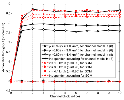
Figure 3: Comparison of achievable throughput of the proposed channel tracking scheme, for both the channel model in (8) and SCM (for several values of $\rho$).

V Conclusion

We proposed a channel tracking scheme tailored for temporally correlated NLoS millimeter wave MIMO channels. The proposed scheme adapts to channel correlation statistics, by constructing well-designed rotation codebooks, and updates the analog precoder and combiner in a mode-by-mode fashion. Simulation results illustrate that the proposed channel tracking scheme outperforms the independent sounding scheme in the presented parametric channel evolution model and the SCM.

References

- [1] E. Torkildson, U. Madhow, and M. Rodwell, “Indoor millimeter wave MIMO: Feasibility and performance,” IEEE Trans. Wireless Commun., vol. 10, no. 12, pp. 4150–4160, Dec 2011.
- [2] S. Hur, T. Kim, D. Love, J. Krogmeier, T. Thomas, and A. Ghosh, “Millimeter wave beamforming for wireless backhaul and access in small cell networks,” IEEE Trans. Commun., vol. 61, no. 10, pp. 4391–4403, Oct 2013.
- [3] M. Marcus and B. Pattan, “Millimeter wave propagation spectrum management implications,” IEEE Microwave Magazine, vol. 6, no. 2, pp. 54–62, Jun 2005.
- [4] A. Alkhateeb, O. El Ayach, G. Leus, and R. Heath, “Channel estimation and hybrid precoding for millimeter wave cellular systems,” IEEE Journal of Selected Topics in Signal Processing, vol. 8, no. 5, pp. 831–846, Oct 2014.
- [5] A. Sayeed and N. Behdad, “Continuous aperture phased MIMO: basic theory and applications,” in Proc. 2010 Allerton Conf. Commun., Control, Comput., Sep 2010, pp. 1196–1203.
- [6] V. Venkateswaran and A.-J. van der Veen, “Analog beamforming in MIMO communications with phase shift networks and online channel estimation,” IEEE Trans. Signal Process., vol. 58, no. 8, pp. 4131–4143, Aug 2010.
- [7] A. Sayeed, “Deconstructing multiantenna fading channels,” IEEE Trans. Signal Process., vol. 50, no. 10, pp. 2563–2579, Oct 2002.
- [8] J. Brady, N. Behdad, and A. Sayeed, “Beamspace MIMO for millimeter-wave communications: System architecture, modeling, analysis, and measurements,” IEEE Trans. Antennas Propag, vol. 61, no. 7, pp. 3814–3827, Jul 2013.
- [9] B. Banister and J. Zeidler, “Feedback assisted transmission subspace tracking for MIMO systems,” IEEE J. Sel. Areas Commun., vol. 21, no. 3, pp. 452–463, Apr 2003.
- [10] J. Yang and D. Williams, “Transmission subspace tracking for MIMO systems with low-rate feedback,” IEEE Trans. Commun., vol. 55, no. 8, pp. 1629–1639, Aug 2007.
- [11] T. Kim, D. Love, and B. Clerckx, “MIMO systems with limited rate differential feedback in slowly varying channels,” IEEE Trans. Commun., vol. 59, no. 4, pp. 1175–1189, Apr 2011.
- [12] “Spatial channel model for multiple input multiple output (MIMO) simulations,” 3GPP TR 25.996 V6.1.0, Sep 2003.
- [13] J. G. Proakis, Digital Communications, 4th ed. McGraw Hill, 2000.
- [14] Y. Kim, X. Li, T. Kim, and D. Love, “Combination lock-like differential codebook for temporally correlated channels,” Electronics Letters, vol. 48, no. 1, pp. 45–47, Jan 2012.
- [15] S. M. Kay, Fundumentals of Statistical Signal Processing: Estimation Theory. Englewood Cliffs, NJ: Prentice-Hall, 1993.