Self-consistence of the Standard Model via the renormalization group analysis

Abstract

A short review of recent renormalization group analyses of the self-consistence of the Standard Model is presented.

1 Introduction

The recent discovery of the Higgs boson [1, 2] at the LHC with mass

$$M_{H} = 125.03^{+0.26}_{-0.27}\mbox{(stat)}{}^{+0.13}_{-0.15}\mbox{(syst)}~{}\mbox{GeV}\;,\quad\mbox{\cite[cite]{[\@@bibref{}{CMS:2014}{}{}]}}$$

$$M_{H} = 125.36\pm 0.37\mbox{(stat)}\pm 0.18\mbox{(syst)}~{}\mbox{GeV}\;,\quad\mbox{\cite[cite]{[\@@bibref{}{ATLAS:2014}{}{}]}}\;,$$

and the fact that so far no signal for new physics has been found, gives rise to the necessity to analyze in detail the self-consistency of the Standard Model. The Higgs boson is a necessary ingredient of the Standard Model (SM), required by its perturbative renormalizability [5, 6]. However, the renormalizability does not give rise to any constraints on the values of parameters of the Lagrangian, but only on the type of interactions. Some additional restrictions on the values of masses and coupling constants are coming from unitarity, triviality and vacuum stability. These three ideas have been used within last decades for an analysis of the self-consistency of the SM.

Unitarity bound: bounds on masses of fermions and Higgs bosons of any renormalizable model can be derived from considerations of the radiative corrections to decays and/or scattering processes [7, 8]. The breakdown of unitary can be avoided by adding a new particles (which implies the existence of new physics) or by the requirement that the perturbative approach must be meaningful (this implies a bound on the particles mass or its coupling constants) [9]. Unitary bounds depend on the type of process under consideration and the precise definition of the breakdown of the perturbative approach. For the Standard Model, the unitary bound for the Higgs boson mass is $M_{H}\lesssim 1~{}\mbox{TeV}\;.$

Triviality and Landau pole: The triviality constraint is related with the high energy behavior of the running couplings. Is it well known, that a running coupling $h(\Lambda)$ may suffers from a Landau pole when the corresponding $\beta$-function is positive:

$$\frac{d}{d\Lambda}h(\Lambda)=\beta_{0}h^{3}(\Lambda)\longrightarrow h^{2}(\Lambda)=\frac{h_{R}^{2}}{1-\beta_{0}h_{R}^{2}\ln\frac{\Lambda}{M}}\;,$$ (1)

where $\Lambda$ is the ultra-violet cutoff, $M$ is a characteristics scale of the process under consideration and $h_{R}$ is the renormalized (running) charge at scale $M$. As follows from Eq. (1), the running coupling $h^{2}(\Lambda)$ diverges at scale $\Lambda_{\mbox{Landau}}$ defined as $\Lambda_{\mbox{Landau}}=M\,\exp\left[\frac{1}{\beta_{0}h_{R}^{2}}\right]\;,$ when $\beta_{0}>0$. In the SM, Landau poles may exists for the $U(1)$-gauge coupling, $g_{1}$, Yukawa couplings, $y_{f}$ and the Higgs self-coupling, $\lambda$. For the most important couplings the SM renormalization group (RG) equations read

$$\frac{dh}{dt}=\frac{1}{16\pi^{2}}\beta_{h}\;,\quad h\in\{g_{1},g_{2},g_{3},y_{f},\lambda\}\;,$$

where in the one-loop approximation the corresponding $\beta$-functions have the following form:

$$\beta_{1}=\frac{41}{6}g_{1}^{3}\;,\quad\beta_{2}=-\frac{19}{6}g_{2}^{3}\;,\quad\beta_{3}=-7g_{3}^{3}\;,\quad\beta_{y_{t}}=y_{t}\biggl{[}\frac{9}{2}y_{t}^{2}-8g_{3}^{2}-\frac{9}{4}g_{2}^{2}-\frac{17}{12}g_{1}^{2}\biggr{]}\;,$$

$$\beta_{\lambda}=\lambda\biggl{[}24\lambda\!+\!12y_{t}^{2}\!-\!9g_{2}^{2}\!-\!3g_{1}^{2}\biggr{]}-{\biggl{[}6y_{t}^{4}\!-\!\frac{9}{8}g_{2}^{4}\!-\!\frac{3}{8}g_{1}^{4}\!-\!\frac{3}{4}g_{1}^{2}g_{2}^{2}\biggr{]}}\;.$$ (2)

It has been shown in [10] that the Landau pole in the Higgs self-coupling $\lambda$ would be below Planck scale if the Higgs is heavier than $180~{}\mbox{GeV}$. The results of recent analyses [11, 12] have confirmed that all coupling constants are free from Landau singularities and have smooth behavior in interval between $M_{Z}\sim 90~{}\mbox{GeV}$ and $M_{Planck}=2.435\times 10^{18}~{}\mbox{GeV}$ (see Fig. 1):

     

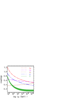
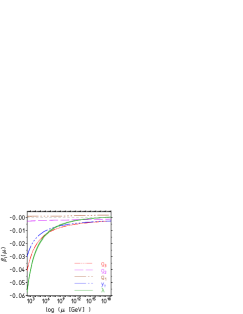
Figure 1: The running coupling constants(left) and corresponding $\beta$-functions (right). The plots are taken from [11].

1.1 Vacuum stability and effective potential

For the analysis of the vacuum stability one needs to recall some basic definitions related with the scalar potential and its generalization in Quantum Field Theory. Let us remind, that at the classical level, the Higgs potential in the SM

$$V(\phi)=\frac{1}{2}m^{2}\phi^{2}+\frac{1}{4!}\lambda\phi^{4}\;,$$ (3)

is bounded from below for $\lambda>0$ and has a trivial minimum for $m^{2}>0$ at $\phi=0$, and non-trivial minima at $\phi^{2}=\frac{-m^{2}}{\lambda}$ for $m^{2}<0$. At the quantum level, instead of the classical potential defined by Eq. (3), the effective potential should be analysed [13]. It can be written in the Landau gauge and the $\overline{\mbox{MS}}$ scheme as [14]

$$V(\phi) \to V_{eff}(\phi(t))=-\frac{1}{2}m^{2}(t)\phi^{2}(t)+\frac{1}{4!}\lambda(t)\phi^{4}(t)+\frac{1}{16\pi^{2}}V_{1}+\frac{1}{(16\pi^{2})^{2}}V_{rest}\;,$$ (4)

where (we use the notations of [15]):

$$V_{1} = \sum_{i}\frac{k_{i}}{4}M_{i}^{4}(\phi(t))\left[\ln\frac{M_{i}^{2}(\phi(t))}{\mu^{2}}-C_{i}\right]\;,$$

$$\phi(t) = \exp\{-\int_{0}^{t}\gamma(\tau)d\tau\}\phi_{clas}\;,\quad M_{i}^{2}(\phi(t))=a_{i}h_{i}(t)\phi(t)^{2}+b_{i}\;,$$ (5)

$h_{i}(t)$ are the running couplings, $\gamma(t)$ is the anomalous dimension of the Higgs field, and $k_{i},C_{i},a_{i},b_{i}$ are numerical constants. By $V_{rest}$ we denote the higher-order contributions, which, in particular, also include the higher dimension operators (it begins at four loop) [14, 16]:

$$V_{rest}\sim\lambda\phi^{4}\sum_{L>4}\left(\frac{\lambda^{2}\phi^{2}}{m^{2}+\frac{1}{2}\lambda\phi^{2}}\right)^{L-3}\;,$$ (6)

where $L$ is the number of loops (for more details see Section 4 of [14] or [17]).

The quantum corrections modify the shape of the effective potential such that a second minimum at large (Planck) scale may be generated. This second minimum (see Fig. (2)) is: (left plot) stable $V_{eff}(v)<V_{eff}(\phi_{\mbox{min}})$, (middle plot) critical (two minima are degenerate in energy) $V_{eff}(v)=V_{eff}(\phi_{\mbox{min}})$, (right plot) unstable/metastable $V_{eff}(v)>V_{eff}(\phi_{\mbox{min}})$, electroweak vacuum and

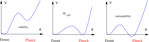
Figure 2: The form of the effective potential for the Higgs field $\phi$ which corresponds to the stable (left), critical (middle) and metastable (right) electroweak vacuum. The plot is taken from [18].

$v$ is the location of the EW minimum and $\phi_{\mbox{min}}$ is the value of a new minimum. Depending on the values of the Higgs boson and top quark masses the lifetime of the EW vacuum can be larger or smaller then the age of the Universe [19, 20, 21]. The first case corresponds to the metastability scenario.

To get practical criteria of stability, the following step-by-step approximations are used [22]: (i) the potential at very high values of the field is dominated by the quartic term $V_{eff}\sim\lambda(\phi)\phi^{4}$ and $\lambda(\phi)$ depends on $\phi$ as the running coupling $\lambda(\mu)$ depends on the running scale $\mu$; (ii) it’s looking the large value of the field $\phi=\phi_{crit}$, where $\lambda(\phi_{crit})=0$; (iii) combine together the previous two approximations, we get at very high values of the Higgs field $\left.V_{eff}\right|_{\phi\sim\phi_{crit}}\simeq\lambda(\phi_{crit})\phi_{crit}^{4}.$ Then, the effective potential becomes negative (unbounded from below) when $\lambda(\mu)<0$ and the vacuum at the EW scale is not the absolute minimum. As follows from Eqs. (2), the Higgs self-coupling $\lambda$ is the only SM dimensionless coupling that can change sign with the scale variation since its beta-function, $\beta_{\lambda}$ contains a part which is not proportional to $\lambda$. In the considered approximation,
the requirement that the electroweak vacuum $<\phi>=(\sqrt{2}G_{F})^{-\frac{1}{2}}=246.22~{}\mbox{GeV}$ is the absolute minimum of the potential up to scale $\Lambda$, implies

$$\lambda(\mu)>0\;,\quad\mbox{for any}\quad\mu<\Lambda\;.$$ (7)

The role of quadratic term or higher dimensional terms (see Eq.(6)) is discussed in Section 3.

2 Analysis

2.1 Renormalization group equations and Matching Conditions

Both the questions, the one concerning vacuum stability and the one concerning triviality, in the Standard Model are reduced to the renormalization group analysis of the Higgs self-coupling $\lambda$. The evolution of $\lambda$ includes the evolution of all coupling constants, see Eq. (2).

The starting point for solving the evolution equations is provided by the matching conditions: the relations between the running coupling constants $h_{i}(\mu)$ and the relevant (pseudo-) physical observables, $\sigma_{i}$. The simplest form for the matching conditions follows when physical masses are taken as the referring point: $\sigma_{i}\equiv M_{i}$. In this case the matching conditions have the following form [23]:

$$h_{i}(\mu^{2})=c_{i}\frac{G_{F}}{\sqrt{2}}M_{i}^{2}\left(1+\delta_{\alpha_{s}}+\delta_{\alpha}+\delta_{\alpha\alpha_{s}}+\delta_{\alpha^{2}}+\delta_{\alpha_{s}^{2}}+\cdots\right)\;,$$ (8)

where $c_{i}$ are normalization constants and $\delta_{\alpha_{j}^{k}}$ are including only propagator type diagrams of order $O(\alpha_{j}^{k})$. The evaluation of the one-loop EW matching conditions of order $O(\alpha)$ was partially done in [23, 24, 25] and has been completed in [26, 27]. The two-loop matching conditions of order $O(\alpha^{2})$ for the Higgs self-coupling $\lambda$ in the limit of heavy Higgs boson have been evaluated in [28, 29], and full two-loop results were completed in [30, 31, 32, 33, 34, 35]. The $O(\alpha\alpha_{s})$ corrections for the top-quark Yukawa coupling within the SM have been evaluated in [36, 37] and $O(\alpha^{2})$ corrections are available only in the gaugeless limit [38, 39]. A state of the art evaluation attempting matching at the two-loop level has been reported in  [12] (results see below).

The evaluation of the 3-loop RG equations for the SM gauge coupling was started in [40, 41], and full 3-loop results for the Standard Model have been published in [42, 43, 44, 45, 46, 47, 48].

2.2 Results of RG analysis

After the top-quark discovery the results of RG analyses of self-consistence of the SM are typically fitted by three parameters and can be written as follows:

$$M_{\mbox{min}}>\left[M_{crit}\!+\!c_{1}\times\left(M_{t}-M_{\mbox{exp}}\right)\!+\!c_{2}\times\left(\alpha_{s}-\alpha_{s,\mbox{exp}}\right)\right]~{}\mbox{GeV}\;,$$ (9)

where $M_{crit}$ is the critical value of the Higgs boson mass, $c_{1},c_{2}$ are some numerical coefficients and $M_{\mbox{exp}}$ and $\alpha_{s,\mbox{exp}}$ are the latest experimental values of the pole mass of the top-quark and of the strong coupling constant, respectively.

The detailed analysis of stability/metastability bounds based on the two-loop RG equations for all SM couplings and one-loop EW matching conditions (as well as two-loop QCD corrections to the top-quark Yukawa coupling $y_{t}$) have been presented in [49]:

$$M_{\mbox{min}}\geq\left[130\!+\!1.8\!\times\!\left(\frac{M_{t}^{\rm pole}\!-\!173.2~{}{\rm GeV}}{0.9~{}{\rm GeV}}\right)\!-\!0.5\!\times\!\left(\frac{\alpha_{s}(M_{Z})\!-\!0.1184}{0.0007}\right)\pm 3\right]~{}\mbox{GeV}\;,$$ (10)

with $M_{t}=(173.2\pm 0.9)~{}\mbox{GeV}$ and $\alpha_{s}(M_{Z})=0.1184\pm 0.0007$ as input parameters and where the error of $3~{}\mbox{GeV}$ is an estimation of unknown higher-order corrections.

The analysis of vacuum stability performed with inclusion of 3-loop RG equations and 2-loop matching conditions was presented in [50] and [51] with the following results:

$$M_{\mbox{min}} \geq \left[128.95\!+\!2.2\!\times\!\left(\frac{M_{t}^{\rm pole}\!-\!172.9~{}{\rm GeV}}{1.1~{}{\rm GeV}}\right)\!-\!0.56\!\times\!\left(\frac{\alpha_{s}(M_{Z})\!-\!0.1184}{0.0007}\right)\pm 1\right]~{}\mbox{GeV}\;,\quad\mbox{\cite[cite]{[\@@bibref{}{Bezrukov:2012}{}{}]}}$$

$$M_{\mbox{min}} \geq \left[129.4+1.4\!\times\!\left(\frac{M_{t}^{\rm pole}\!-\!173.1~{}{\rm GeV}}{0.7~{}{\rm GeV}}\right)-0.5\!\times\!\left(\frac{\alpha_{s}(M_{Z})\!-\!0.1184}{0.0007}\right)\pm 0.7\right]~{}\mbox{GeV}\;,\quad\mbox{\cite[cite]{[\@@bibref{}{Degrassi:2012}{}{}]}}$$

The latest published analysis have been presented in [12]:

$$M_{\mbox{min}}>\left[129.6\!+\!2.0\!\times\!\left(M_{t}^{\rm pole}\!-\!173.35~{}{\rm GeV}\right)\!-\!0.5\!\times\!\left(\frac{\alpha_{s}(M_{Z})\!-\!0.1184}{0.0007}\right)\pm 0.3\right]~{}\mbox{GeV}\;.$$ (13)

2.3 The analysis of uncertainties

As follows from Eqs. (10)-(13) adding two-loop matching conditions and 3-loop RG equations does not changed dramatically the central value of critical mass: $130\to\sim 129.0\div 129.6$, but essentially reduces the theoretical uncertainties: $(3\to 0.3)~{}\mbox{GeV}$. Adding the leading 3-loop corrections to the matching conditions for the Higgs self-coupling [52, 53] does not modified the final result, Eq. (13). The $3\sigma$ variations of $\alpha_{s}$ or the small variation of the value of the matching scale [54] also do not produce the significant corrections to the fitted expression.

The main error in Eqs. (10)-(13) is coming from the input value of top-quark mass: $\Delta M_{\mbox{min}}\sim 2.0\!\times\!\Delta M_{t}^{\rm pole}.$ Currently the most precise measurement of the top-quark mass has been reported as the world combination of the ATLAS, CDF, CMS and D0 [56] (for completeness we present also the result based only on CDF/D0 data [55]):

$$M_{t} = 173.18\pm 0.94~{}\mbox{GeV}\;,\quad\mbox{\cite[cite]{[\@@bibref{}{top:2012}{}{}]}}$$ (14)

$$M_{t} = 173.76\pm 0.76~{}\mbox{GeV}\;,\quad\mbox{\cite[cite]{[\@@bibref{}{top}{}{}]}}$$ (15)

It has been pointed out in [57] that the values of the top quark mass quoted by the experimental collaborations correspond to parameters in Monte Carlo event generators in which, apart from parton showering, the partonic subprocesses are calculated at the tree level, so that a rigorous theoretical definition of the top quark mass is lacking (see more detailed discussion of this issue in [58]). In particular, the following issues in precision top mass determination at hadron colliders are relevant [59]: MC modeling, reconstruction of the top pair, unstable top and finite top width effects, bound-state effects in top pair production at hadron colliders, renormalon ambiguity in top mass definition, alternative top mass definitions, higher-order corrections, non-perturbative corrections, contributions from physics beyond the Standard Model.

To reduce the uncertainties related with undetermined differences between Monte-Carlo and pole masses (it was estimated in [57, 58] as $1~{}\mbox{GeV}$) the mass of top-quark can be extracted directly from a measurement of the total top-pair production cross section $\sigma_{\mbox{exp}}(p\bar{p}\to t\bar{t}\!+\!X)$. Such analysis performed in [60] with NNLO accuracy with inclusion of the full theoretical uncertainties (the scale variation as well as the (combined) PDF and $\alpha_{s}$ uncertainties) gives rise to the following result, ${M_{t}^{\rm pole}=173.3\pm 2.8~{}\mbox{GeV}}\;.$ The central value is very close to the one in Eq. (15), but the theoretical uncertainty is much larger. Similar analyses (direct extraction of the pole mass of top-quark from measured total cross section) have been performed by a few other groups [61, 62, 63, 64, 58] with the following results:

$$M_{t}^{\rm pole} = 171.4^{+5.4}_{-5.7}~{}\mbox{GeV}\quad\mbox{\cite[cite]{[\@@bibref{}{TOPIXS}{}{}]}}\;,$$ (16)

$$M_{t}^{\rm pole} = 174.3^{+4.9}_{-4.4}~{}\mbox{GeV}\quad\mbox{\cite[cite]{[\@@bibref{}{TOPIXS2013}{}{}]}}\;,$$ (17)

$$M_{t}^{\rm pole} = 174.2^{+3.6}_{-3.9}~{}\mbox{GeV}\quad\mbox{\cite[cite]{[\@@bibref{}{Sbornik}{}{}]}}\;,$$ (18)

$$M_{t}^{\rm pole} = 171.2\pm 2.4\pm 0.7~{}\mbox{GeV}\quad\mbox{\cite[cite]{[\@@bibref{}{ABM:2013}{}{}]}}\;,$$ (19)

where the full NNLO QCD corrections evaluated in [65, 66] have been combined with the soft-gluon resummation at NNLL accuracy [63] and Coulomb-gluon NNLL resummation [61]. All results in Eqs. (16)-(19) have large theoretical uncertainties. To improve the current precision of the top-mass determination from the total cross section the higher order corrections as well as a reduction of PDF and $\alpha_{s}$ uncertainties are required [67, 68].

3 Some additional sources of uncertainties

3.1 EW contribution to the running mass of the top-quark

In order to achieve percent level precision theoretical predictions for cross section $\sigma_{pp\to t\bar{t}}$ not only QCD NNLO radiative corrections should be applied. The EW part as well as mixed EW $\times$ QCD corrections have to be included in a systematic way. For example, the QCD interaction is not responsible for the non-zero width of the top-quark, which can be understood precisely only by inclusion of the EW interactions. In any case, the EW effect [69, 70] as well as the non-zero width should be included in addition to the QCD corrections [71].

In contrast to QCD, where the mass of a quark is the parameter of the Lagrangian, the notion of $\overline{\mbox{MS}}$-mass in EW theory is not determined entirely by the prescriptions of minimal subtraction. It depends on the value of vacuum expectation value $v(\mu^{2})$ chosen as a parameter of the calculations so that the running mass is $m_{t}(\mu^{2})=1/\sqrt{2}y_{f}(\mu^{2})v(\mu^{2})$. It has been shown in a series of papers [72, 73, 74] that in the scheme with explicit inclusion of tadpoles [25] the RGE for the running vacuum expectation value $v_{MS}^{2}(\mu^{2})$ which is defined as (see Section 4 in [36])

$$v_{MS}^{2}(\mu^{2})=\frac{1}{\sqrt{2}G_{F}}\frac{1}{1-\overline{\Delta}r}\Biggl{[}\frac{m_{W}^{2}(\mu^{2})}{M_{W}^{2}}\Biggr{]}\Biggl{[}\frac{\alpha(M_{Z})}{\alpha_{MS}(\mu^{2})}\Biggr{]}\Biggl{[}\frac{\sin^{2}\theta^{MS}_{W}(\mu^{2})}{\sin^{2}\theta_{W}^{OS}}\Biggr{]}\;,$$ (20)

coincides with RGE for the classical definition of tree-level scalar potential vacuum

$$\mu^{2}\frac{d}{d\mu^{2}}v_{MS}^{2}(\mu^{2})=\mu^{2}\frac{d}{d\mu^{2}}\left[\frac{m^{2}(\mu^{2})}{\lambda(\mu^{2})}\right]\;,$$ (21)

where $m^{2}$ and $\lambda$ are the parameters of the scalar potential, see Eq. (3). The asymptotic behavior and properties of this vacuum at low and high energies have been analysed in [75, 76]. In particular, for a current values of Higgs and top-quark masses an IR point $\mu_{IR}$ close to the value of the Z-boson mass exist such that $\left.v_{MS}^{2}(\mu^{2})\right|_{\mu\sim M_{Z}}=(\sqrt{2}G_{F})^{-1/2}=246.22~{}\mbox{GeV}$ (see details in [76]). In the framework of the effective potential approach, a similar condition for the minimum of effective potential is imposed by hand (see details in [15]).

In the SM the decoupling theorem [77] is not valid in the week sector, the “decoupling by hand” prescription does not work and we have to take full SM parameter relations as they are. In this approximation we got [75] that the EW contribution is large and has opposite sign relative to the QCD contributions, so that the total SM correction is small and approximately equal to $M_{t}-m_{t}(m_{t})\sim 1\div 2~{}\mbox{GeV}$ (see left plot in Fig. (3)). The complete $O(\alpha^{2})$ correction to the relation between pole and $\overline{\mbox{MS}}$  masses of the top-quark are not yet available, but our numerical estimation [75] is in agreement with result of [38, 39] and it is of the order of the $O(\alpha_{s}^{4})$ corrections [78, 79]. For the evaluation of the NNLO corrections three different schemes have been used: with explicit inclusion of tadpole [72, 73, 74], the so called $\beta$-renormalization scheme [33, 34, 35], and the method of minimization of the effective potential [12, 51, 80]. The equivalence of these three methods of evaluation of matching conditions have never been analyzed. In particular, the structure of 2-loop UV-counterterms in [72, 73, 74] and [33, 34] are different; the gauge dependence of the effective potential method versus gauge independence of the scheme including the tadpoles [72, 73, 74] (the gauge (in)dependence of prediction of the critical value of the Higgs boson mass via effective potential scheme have been analysed in [81, 82]), etc. The difference between these methods is of order $O(G_{F}^{2}M_{W}^{4})$ and may reach the value $\sim 10^{-3}\div 10^{-4}$. Another source of numerical difference is related with the choice between complex mass [35] or pole mass [72, 74] in Eq. (8). It is equivalent to systematic additional uncertainty of order $O(\Gamma^{2}/(4M^{2}))$ (see discussion in [83, 37]), where $\Gamma$ is the width and $M$ is the mass of particle. This effect is the most significant for the top-quark Yukawa-coupling: $\delta y_{f}\sim 1/173^{2}=3\times 10^{-5}$. The unknown QCD corrections of order $O(\alpha_{s}^{4})$ to the top-quark Yukawa-coupling is $\delta_{\alpha_{s}^{4}}y_{f}\sim 1\times 10^{-3}$ [78, 79]. The two-loop EW correction $\delta_{\alpha^{2}}y_{t}(\mu=M_{t})\approx\frac{5}{(4\pi)^{2}}=6\times 10^{-4}$ (see Eq.(2.49) in [12]) and three-loop corrections can be estimated as $\delta_{\alpha_{s}^{2}\alpha}y_{t}(\mu=M_{t})\sim[\delta_{\alpha_{s}^{2}}y_{t}(\mu=M_{t})]\times[\delta_{\alpha}y_{t}(\mu=M_{t})]=0.011\times 0.00135=1.5\times 10^{-5}$. All these effects do not change the central value of the critical mass of the Higgs boson, Eqs. (10)-(13), but affect the value of theoretical uncertainties.

     

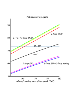
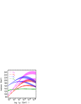
Figure 3: The running top-quark mass at low value of $\mu$ (left) and behavior of running masses at large values of $\mu$ (right). At the right the bands corresponds to Higgs mass in interval $124~{}\mbox{GeV}<M_{H}<127~{}\mbox{GeV}$. The right plot is taken from [11].

3.2 The first order phase transition and quadratic divergences

It was pointed out in [11] that in the region where the Higgs self-coupling is positive and close to zero, $\lambda(\Lambda)\sim 0$, the quadratic term of effective potential may start play the essential role since $\lambda(\Lambda)\phi^{2}(\Lambda)\ll m^{2}(\Lambda).$ The massive parameter $m^{2}$ suffers from quadratic divergences: $\Delta m^{2}(\Lambda)=\frac{\Lambda^{2}}{16\pi^{2}}Q_{1}\;,$ where the coefficients $Q_{1}$ are expressible in terms of coupling constants [84], $Q_{1}=\lambda+\frac{1}{8}g_{1}^{2}+\frac{3}{8}g_{2}^{2}-y_{t}^{2}\;.$ The coefficient $Q_{1}$ may vanish at some high scale $\Lambda^{*}$ [85]. If $\Lambda\sim\Lambda^{*}$ then $m^{2}$-term may change the sign and that leads to a phase transition of the first order restoring the EW symmetry [11]. Realization of this scenario (the value of scale where $Q_{1}=0$) strongly depends on the value of top-quark mass (see discussion in [86, 87]). The Higgs inflation and hierarchy problem within this scenario have been discussed in [88, 89].

3.3 Inclusion of higher dimension operators

As well known [14] the effective potential contains also the higher dimensional operators (see Eq. (6)). The impact of new physics interaction at Planck scale was analysed in [90] by adding two higher dimensional operators $\phi^{6}$ and $\phi^{8}$ suppressed by inverse powers of Planck scale $M_{Planck}$ to the Higgs potential. It has been shown that higher dimension operators may change the lifetime of the metastable vacuum, $\tau$, from $\tau=1.49\times 10^{714}T_{U}$ to $\tau=5.45\times 10^{-212}T_{U}$, where $T_{U}$ is the age of the Universe.

4 Conclusion

The main results of the LHC is the discovery of the Higgs boson. The second important result is the absence of a signal of new physics. After the Higgs boson discovery the Standard Model is completed. Since all parameters of the Standard Model are defined now experimentally, one can analyze the extrapolation of the SM up to the Planck scale. The results of the recent analysis can be summarized as follows:

• The Standard Model is a self-consistent QFT that can be extrapolated from $M_{W}$ to $M_{Planck}$ since all SM couplings remain perturbative (no Landau pole) in that range, see Fig. 1.

• With the current precision in $M_{H}(\sim 126~{}\mbox{GeV})$ , the value of top-quark mass in accordance with CDF/DO/CMS/ATLAS $M_{t}(\sim 173~{}\mbox{GeV})$ and 3-loop RG functions and 2-loop matching conditions, one concludes that the EW vacuum would most likely be metastable [12]: the stability condition is $M_{H}>(129.6\pm 1.5)~{}\mbox{GeV}$ for a given value of top-quark mass. In terms of top quark mass, the stability bound is [22] $M_{t}<(171.36\pm 0.46)~{}\mbox{GeV}.$

• It was shown in [49] that the lifetime of the electroweak vacuum is longer than the age of the Universe for $M_{H}>111~{}\mbox{GeV}$ so that
  Metastability of vacuum with very long lifetime cannot be used as motivation for a New Physics
  A lot of effort has been made recently to analyzed EW vacuum during inflation [91, 92]. The condition of vacuum (meta)stability imposes the constraint on the rate of inflationary expansion that are in tension with BICEP2 result [93]. However, the recent result from the Plank collaboration [94] does not confirm the BICEP2 result [93] so that the further experimental verification is necessary.

• The result of the recent analysis [60] reveals a large theoretical uncertainties in the value of top-quark mass (see Eqs. (16)-(19)). This leads to a large uncertainty $\sim 5~{}\mbox{GeV}$ in the critical value of the Higgs boson mass.

• The mass of the Higgs boson is very close to the values of “critical Higgs mass”, $M_{crit}$: the “multiple point principle” [95], Higgs inflation [96, 97, 98], asymptotic safety scenario [99] The explicit realization $M_{H}=M_{crit}$ would be a strong indication for the absence of a new physics scale between the Fermi and Planck scales.

• To clarify the situation, more precise measurements of the coupling constants $\alpha_{s},\lambda,y_{t}$ are needed. Unfortunately, there are no ways of directly measuring the Higgs self-coupling and top-quark Yukawa coupling with high precision in the immediate future [100, 101, 102, 103].

• The higher order calculations are also desirable.

Therefore,
precision determinations of parameters are more important than ever and a real challenge for experiments at the LHC and at a future ILC.

5 Acknowledgments

We are thankful to S.Alekhin, A.Arbuzov, F.Bezrukov and S.Moch for the stimulating discussions. MYK would like to thank the organizers of the conference ACAT2014 and specially to Andrei Kataev, Grigory Rubtsov and Milos Lokajicek for the invitation and for creating such a stimulating atmosphere. The authors are indebted to anonymous referee for constructive and valuable comments. This work was supported in part by the German Federal Ministry for Education and Research BMBF through Grant No. 05 H12GUE, by the German Research Foundation DFG through the Collaborative Research Center No. 676 Particles, Strings and the Early Universe—The Structure of Matter and Space-Time.

References

References

- [1] Aad G et al. [ATLAS Collaboration] 2012 Phys. Lett. B 716 1 (Preprint 1207.7214)
- [2] Chatrchyan S et al. [CMS Collaboration] 2012 Phys. Lett. B 716 30 (Preprint 1207.7235)
- [3] [CMS Collaboration] 2014 Precise determination of the mass of the Higgs boson and studies of the compatibility of its couplings with the standard model (Preprint CMS-PAS-HIG-14-009)
- [4] G. Aad et al. [ATLAS Collaboration], Phys. Rev. D 90 052004 (Preprint 1406.3827)
- [5] ’t Hooft G 1971 Nucl. Phys. B 35 167
- [6] ’t Hooft G and Veltman M J G 1972 Nucl. Phys. B 44 189
- [7] Dicus D A and Mathur V S 1973 Phys. Rev. D 7 3111
- [8] Lee B W, Quigg C and Thacker H B 1977 Phys. Rev. D 16 1519
- [9] Vetlman M J G 1977 Acta Phys. Polon. B 8 475
- [10] Hambye T and Riesselmann K 1997 Phys. Rev. D 55 7255 (Preprint 9610272)
- [11] Jegerlehner F 2014 Acta Phys. Polon. B 45 1167 (Preprint 1304.7813)
- [12] Buttazzo D et al. 2013 JHEP 1312 089 (Ppreprint 1307.3536)
- [13] Coleman S R and Weinberg E J 1973 Phys. Rev. D 7 1888
- [14] Ford C et al. 1993 Nucl. Phys. B 395 17 (Preprint 9210033)
- [15] Casas J A et al. 1995 Nucl. Phys. B 436 3 [Erratum-ibid. B 439 (1995) 466] (Preprint 9407389)
- [16] Nakano H and Yoshida Y 1994 Phys. Rev. D 49 5393 (Preprint 9309215)
- [17] Einhorn M B and Jones D R T 2007 JHEP 0704 051 (Preprint 0702295)
- [18] Shaposhnikov M 2013 PoS EPS -HEP2013 155 (Preprint 1311.4979)
- [19] Coleman S R 1977 Phys. Rev. D 15 2929 [Erratum-ibid. D 16 (1977) 1248].
- [20] Callan C G and Coleman S R 1977 Phys. Rev. D 16 1762
- [21] Arnold P B 1989 Phys. Rev. D 40 613
- [22] Espinosa J R 2013 Vacuum Stability and the Higgs Boson (Preprint 1311.1970)
- [23] Sirlin A and Zucchini R 1986 Nucl. Phys. B 266 389
- [24] Sirlin A 1980 Phys. Rev. D 22 971
- [25] Fleischer J and Jegerlehner F 1981 Phys. Rev. D 23 2001
- [26] Böhm M, Spiesberger H and Hollik W 1986 Fortsch. Phys. 34 687
- [27] Hempfling R and Kniehl B A 1995 Phys. Rev. D 51 1386
- [28] van der Bij J and Veltman M J G 1984 Nucl. Phys. B 231 205
- [29] Ghinculov A and van der Bij J J 1995 Nucl. Phys. B 436 30
- [30] Awramik M et al. 2004 Phys. Rev. D 69 053006 (Preprint 0311148)
- [31] Aglietti U et al. 2004 Phys. Lett. B 595 432 (Preprint 0404071)
- [32] Degrassi G and Maltoni F 2004 Phys. Lett. B 600 255 (Preprint 0407249)
- [33] Actis S and Passarino G 2007 Nucl. Phys. B 777 35 (Preprint 0612123)
- [34] Actis S and Passarino G 2007 Nucl. Phys. B 777 100 (Preprint 0612124)
- [35] Actis S et al. 2008 Phys. Lett. B 670 12 (Preprint 0809.3667)
- [36] Jegerlehner F and Kalmykov M 2003 Acta Phys. Polon. B 34 5335 (Preprint 0310361)
- [37] Jegerlehner F and Kalmykov M 2004 Nucl. Phys. B 676 365 (Preprint 0308216)
- [38] Martin S P 2005 Phys. Rev. D 72 096008
- [39] Kniehl B A and Veretin O V 2014 Nucl. Phys. B 885 459 (Preprin 1401.1844)
- [40] Kazakov D I, Tarasov O V and Vladimirov A A 1979 Sov. Phys. JETP 50 521
- [41] Tarasov O V, Vladimirov A A and Zharkov A Y 1980 Phys. Lett. B 93 429
- [42] Mihaila L N, Salomon J and Steinhauser M 2012 Phys. Rev. Lett. 108 151602 (Preprin 1201.5868)
- [43] Mihaila L N, Salomon J and Steinhauser M 2012 Phys. Rev. D 86 096008 (Preprint 1208.3357)
- [44] Chetyrkin K G and Zoller M F 2012 JHEP 1206 033
- [45] Bednyakov A V, Pikelner A F and Velizhanin V N 2013 JHEP 1301 017 (Preprint 1210.6873)
- [46] Bednyakov A V, Pikelner A F and Velizhanin V N 2013 Phys. Lett. B 722 336 (Preprin 1212.6829)
- [47] Bednyakov A V, Pikelner A F and Velizhanin V N 2013 Nucl. Phys. B 875 552 (Preprint 1303.4364)
- [48] Chetyrkin K G and Zoller M F 2013 JHEP 1304 091 [Erratum-ibid. 1309 155] (Preprint 1303.2890)
- [49] Elias-Miro J et al. 2012 Phys. Lett. B 709 222 (Preprint1112.3022)
- [50] Bezrukov F et al. 2012 JHEP 1210 140 (Preprint 1205.2893)
- [51] Degrassi G et al. 2012 JHEP 1208 098 (Preprint 1205.6497)
- [52] Martin S P 2014 Phys. Rev. D 89 013003 (Preprint 1310.7553)
- [53] Martin S P and Robertson D G 2014 (Preprint 1407.4336)
- [54] Masina I 2012 Phys. Rev. D 87 053001 (Preprint 1209.0393)
- [55] T. Aaltonen et al. [CDF and D0 Collaborations] 2012 Phys. Rev. D 86 092003 (Preprint 1207.1069)
- [56] [ATLAS and CDF and CMS and D0 Collaborations] 2014 First combination of Tevatron and LHC measurements of the top-quark mass (Preprint 1403.4427)
- [57] Hoang A H and Stewart I W 2008 Nucl. Phys. Proc. Suppl. 185 220 (Preprint 0808.0222)
- [58] Moch et al. 2014 High precision fundamental constants at the TeV scale (Preprint 1405.4781)
- [59] Juste A et al. 2013 Determination of the top quark mass circa 2013: methods, subtleties, perspectives (Preprint 1310.0799)
- [60] Alekhin S, Djouadi A and Moch S 2012 Phys. Lett. B 716 214
- [61] Beneke et al. 2012 JHEP 1207 194 (Preprint 1206.2454)
- [62] Beneke et al. 2013 Nucl. Phys. Proc. Suppl. 234 101 (Preprint 1208.5578)
- [63] Czakon M and Mitov M 2014 Comput. Phys. Commun. 185 2930 (Preprint 1112.5675)
- [64] Alekhin S, Blümlein J and Moch S 2014 Phys. Rev. D 89 054028 (Preprint 1310.3059)
- [65] Bärnreuther P, Czakon M and Mitov A 2012 Phys. Rev. Lett. 109 132001 (Preprint 1204.5201)
- [66] Czakon M, Fiedler P and Mitov A 2013 Phys. Rev. Lett. 110 252004 (Preprint 1303.6254)
- [67] Czakon M et al. 2013 JHEP 1307 167 (Preprint 1303.7215)
- [68] Ball R D et al. [The NNPDF Collaboration] 2014 Parton distributions for the LHC Run II (Preprint 1410.8849)
- [69] Beenakker W et al. 1994 Nucl. Phys. B411 343
- [70] Kühn J H, Scharf A and Uwer P 2007 Eur. Phys. J. C51 37 (Preprint 0610335)
- [71] Falgari P, Papanastasiou A S and Signer A 2013 JHEP 1305 156 (Preprint 1303.5299)
- [72] Jegerlehner F, Kalmykov M and Veretin O 2002 Nucl. Phys. B 641 285 (Preprint 0105304)
- [73] Jegerlehner F, Kalmykov M and Veretin O 2003 Nucl. Phys. Proc. Suppl. 116 382 (Preprint 0212003)
- [74] Jegerlehner F, Kalmykov M and Veretin O 2003 Nucl. Phys. B 658 49 (Preprint 0212319)
- [75] Jegerlehner F, Kalmykov M and Kniehl B A 2013 Phys. Lett. B 722 123 (Preprint 1212.4319)
- [76] Jegerlehner F, Kalmykov M and Kniehl B A 2013 PoS DIS 2013 190 (Preprint 1307.4226)
- [77] Appelquist A and Carazzone J 1975 Phys. Rev. D 11 2856
- [78] Kataev A L and Kim V T 2010 Phys. Part. Nucl. 41 946 (Preprint 1001.4207)
- [79] Sumino Y 2014 Phys. Lett. B 728 73 (Preprint 1309.5436)
- [80] Martin S P 2004 Phys. Rev. D 70 016005 (Preprint 0312092)
- [81] Loinaz W and Willey R S 1997 Phys. Rev. D 56 7416 (Preprint 9702321)
- [82] Di Luzio L and Mihaila L 2014 JHEP 1406 079 (Preprint 1404.7450)
- [83] Smith M C and Willenbrock S S 1997 Phys. Rev. Lett. 79 3825 (Preprint 9612329)
- [84] Veltman M J G 1981 Acta Phys. Polon. B 12 437
- [85] Hamada Y, Kawai H and Oda K 2013 Phys. Rev. D 87 053009 (Preprint 1210.2538)
- [86] Masina I and Quiros M 2013 Phys. Rev. D 88 093003 (Preprint 1308.1242)
- [87] Jones D R T 2013 Phys. Rev. D 88 098301 (Preprint 1309.7335)
- [88] Jegerlehner F 2014 Acta Phys. Polon. B 45 1215 (Preprint 1402.3738)
- [89] Jegerlehner F 2013 The hierarchy problem of the electroweak Standard Model revisited, (Preprint 1305.6652)
- [90] Branchina V and Messina E 2013 Phys. Rev. Lett. 111 241801 (Preprint 1307.5193)
- [91] Kobakhidze A and Spencer-Smith A 2013 Phys. Lett. B 722 130 (Preprint 1301.2846)
- [92] Enqvist E, Meriniemi T and Nurmi S 2014 JCAP 1407 (2014) 025 (Preprint 1404.3699)
- [93] Ade P A R et al. [BICEP2 Collaboration] 2014 Phys. Rev. Lett. 112 241101 (Preprint 1403.3985)
- [94] Adam R et al. [Planck Collaboration] 2014 Planck intermediate results. XXX. The angular power spectrum of polarized dust emission at intermediate and high Galactic latitudes (Preprint 1409.5738)
- [95] Froggatt C D and and Nielsen H B 1996 Phys. Lett. B 368 96 (Preprint 9511371)
- [96] Bezrukov F L and Shaposhnikov M 2008 Phys. Lett. B 659 703 (Preprint 0710.3755)
- [97] Hamada Y et al. 2014 Phys. Rev. Lett. 112 241301 (Preprint 1403.5043)
- [98] Bezrukov F and Shaposhnikov M 2014 Higgs inflation at the critical point (Preprint 1403.6078)
- [99] Shaposhnikov M and Wetterich C 2010 Phys. Lett. B 683 196 (Preprint 0912.0208)
- [100] Dawson S et al 2013 Working Group Report: Higgs Boson (Preprint 1310.8361)
- [101] Englert C et al. 2014 J. Phys. G 41 113001 (Preprint 1403.7191)
- [102] Bechtle P et al. 2014 Probing the Standard Model with Higgs signal rates from the Tevatron, the LHC and a future ILC (Preprint 1403.1582)
- [103] Baak M et al. [Gfitter Group Collaboration] 2014 Eur. Phys. J. C 74 3046 (Preprint 1407.3792)