A real sextic surface with $45$ handles

Abstract

It follows from classical restrictions on the topology of real algebraic varieties that the first Betti number of the real part of a real nonsingular sextic in $\mathbb{CP}^{3}$ can not exceed $94$. We construct a real nonsingular sextic $X$ in $\mathbb{CP}^{3}$ satisfying $b_{1}(\mathbb{R}X)=90$, improving a result of F.Bihan. The construction uses Viro’s patchworking and an equivariant version of a deformation due to E.Horikawa.

1 Introduction

A real algebraic variety is a complex algebraic variety $X$ equipped with an antiholomorphic involution $c:X\rightarrow X$. Such an antiholomorphic involution is called a real structure on $X$. The real part of $(X,c)$, denoted by $\mathbb{R}X$, is the set of points fixed by $c$. The standard real structure $c_{0}$ on $(\mathbb{C}^{*})^{n}$ is defined by

$$c_{0}(Z_{1},...,Z_{n})=(\overline{Z_{1}},...,\overline{Z_{n}}).$$

The standard real structure on a toric variety of dimension $n$ is the real structure induced by the standard real structure on $(\mathbb{C}^{*})^{n}$. In this text, the only real structures we consider on toric varieties are standard real structures. A real subvariety of a toric variety is a subvariety stable by the standard real structure. For example, a real algebraic surface in $\mathbb{CP}^{3}$ is the zero set of a real homogeneous polynomial in $4$ variables. Unless otherwise specified, all varieties considered are nonsingular. The homology is always considered with $\mathbb{Z}/2\mathbb{Z}$-coefficients. For a topological space $A$, we put $b_{i}(A)=\dim_{\mathbb{Z}/2\mathbb{Z}}H_{i}(A,\mathbb{Z}/2\mathbb{Z})$. The numbers $b_{i}(A)$ are called Betti numbers $($with $\mathbb{Z}/2\mathbb{Z}$ coefficients$)$ of $A$. All polytopes considered are convex lattice polytopes in $\mathbb{R}^{n}$.
Let us remind several classical inequalities and congruences in topology of real algebraic varieties.

Smith-Thom inequality and congruence: Let $X$ be a compact real algebraic variety. Then

$$b_{*}(\mathbb{R}X)\leq b_{*}(X)\mbox{ and }b_{*}(\mathbb{R}X)\equiv b_{*}(X)\mod 2,$$

where $b_{*}$ is the sum of all Betti numbers. The variety $X$ is called an $M$-variety if $b_{*}(\mathbb{R}X)=b_{*}(X)$ and an $(M-a)$-variety if $b_{*}(\mathbb{R}X)=b_{*}(X)-2a$.

Petrovsky-Oleinik inequalities: Let $X$ be a compact complex Kähler manifold of real dimension $4n$ equipped with a real structure. Then

$$2-h^{n,n}(X)\leq\chi(\mathbb{R}X)\leq h^{n,n}(X),$$

where $\chi$ denotes the Euler caracteristic and $h^{p,q}$ denotes the $(p,q)$-Hodge number.

Rokhlin congruence: Let $X$ be a compact $M$-variety of real dimension $4n$. Then

$$\chi(\mathbb{R}X)\equiv\sigma(X)\mod 16,$$

where $\sigma(X)$ is the signature of $X$.

Gudkov-Kharlamov congruence: Let $X$ be a compact ($M-1$)-variety of real dimension $4n$. Then

$$\chi(\mathbb{R}X)\equiv\sigma(X)\pm 2\mod 16.$$

For an introduction concerning restrictions on the topology of real algebraic varieties, see  [Wil78] or  [DK00].
Let $X$ be a compact connected simply-connected projective real surface. From the Smith-Thom inequality and the Petrovsky-Oleinik inequalities, one can deduce bounds for $b_{0}(\mathbb{R}X)$ and $b_{1}(\mathbb{R}X)$ in terms of Hodge numbers of $X$:

$$b_{0}(\mathbb{R}X)\leq\frac{1}{2}(h^{2,0}(X)+h^{1,1}(X)+1),$$ (1)

$$b_{1}(\mathbb{R}X)\leq h^{2,0}(X)+h^{1,1}(X).$$ (2)

These bounds are not sharp in general. One can then ask the following questions.

Question 1.

What is the maximal possible value of $b_{0}(\mathbb{R}X)$ for a real algebraic surface $X$ in $\mathbb{CP}^{3}$ of a given degree?

Question 2.

What is the maximal possible value of $b_{1}(\mathbb{R}X)$ for a real algebraic surface $X$ in $\mathbb{CP}^{3}$ of a given degree?

If the degree is greater than $4$, these questions are still widely open. In 1980, O.Viro formulated the following conjecture.

Conjecture.

$($O.Viro$)$
Let $X$ be a compact connected simply-connected projective real surface. Then

$$b_{1}(\mathbb{R}X)\leq h^{1,1}(X).$$

This conjecture was an attempt to give an answer to Question 2. When $X$ is the double covering of $\mathbb{CP}^{2}$ ramified along a curve of an even degree, this conjecture is a reformulation of Ragsdale’s conjecture (see  [Vir80]). The first counterexample to Ragsdale’s conjecture was constructed by I.Itenberg (see  [Ite93]) using Viro’s combinatorial patchworking (see Section 2 or  [Ite97] or  [Bih99]). This first counterexample opened the way to various counterexamples to Viro’s conjecture and constructions of real algebraic surfaces with many connected components (see  [Ite97],  [Bih99],  [Bih01],  [Bru06],  [IK96] and  [Ore01]). It is not known whether Viro’s conjecture is true for $M$-surfaces.
In the case where $X$ is a real algebraic surface of degree $d$ in $\mathbb{CP}^{3}$, inequalities (1) and (2) specialize to the following ones:

$$b_{0}(\mathbb{R}X)\leq\frac{5}{12}d^{3}-\frac{3}{2}d^{2}+\frac{25}{12}d,$$ (1’)

$$b_{1}(\mathbb{R}X)\leq\frac{5}{6}d^{3}-3d^{2}+\frac{25}{6}d-1.$$ (2’)

Consider the case where $X$ has degree $6$. Then $h^{1,1}(X)=86$, and the inequality (2’), combined with Petrovsky-Oleinik inequalities and Rokhlin congruence, gives $b_{1}(\mathbb{R}X)\leq 94$. F.Bihan constructed in  [Bih99], using Viro’s combinatorial patchworking, a real sextic $X$ satisfying $b_{1}(\mathbb{R}X)=88$. Moreover, the real part of $X$ is homeomorphic to $6S\amalg S_{2}\amalg S_{42}$, where $S$ denotes a $2$-dimensional sphere and $aS_{\alpha}$ denotes the disjoint union of $a$ spheres each having $\alpha$ handles. In this note, we improve this construction.

Theorem 1.

There exists a real sextic surface $X$ in $\mathbb{CP}^{3}$ satisfying $b_{1}(\mathbb{R}X)=90$ such that

$$\mathbb{R}X\simeq 4S\amalg 2S_{2}\amalg S_{41}.$$

The paper is organized as follows. In Sections 2 and 3, we remind Viro’s method and some results about the Euler caracteristic of T-surfaces. In Section 4, we describe a class of real algebraic surfaces, the so-called surfaces of type $(1c)$, and an equivariant deformation of a real surface of type $(1c)$ to a real sextic surface. In Section 5, we use Viro’s combinatorial patchworking to construct a real surface $Z$ of type $(1c)$. Then, using the general Viro’s method, we slightly modify the construction of $Z$ to obtain a real surface $Y$ of type $(1c)$ satisfying

$$\mathbb{R}Y\simeq 4S\amalg 2S_{2}\amalg S_{41}.$$

The existence of a real sextic surface $X$ satisfying $92\leq b_{1}(\mathbb{R}X)\leq 94$ is still unknown.

Acknowledgments. I am very grateful to Erwan Brugallé and Ilia Itenberg for useful discussions and advisements.

2 Viro’s method

2.1 T-construction

The combinatorial patchworking construction (or T-construction) works in any dimension.
Let $(u_{1},...,u_{n})$ be coordinates in $\mathbb{R}^{n}$, and let $\Delta$ be a $n$-dimensional polytope in $\mathbb{R}_{+}^{n}$, where $\mathbb{R}_{+}=\{x\in\mathbb{R}\mbox{ }|\mbox{ }x\geq 0\}$. Denote by $\mathit{Tor}(\Delta)$ the toric variety associated with $\Delta$. We denote by $\mathbb{R}\mathit{Tor}(\Delta)$ the real part of $\mathit{Tor}(\Delta)$ for the standard real structure. Take a triangulation $\tau$ of $\Delta$ with vertices having integer coordinates, and a distribution of signs at the vertices of $\tau$. Denote the sign at any vertex $(i_{1},...,i_{n})$ by $\delta_{i_{1},...,i_{n}}$. For $\epsilon=(\epsilon_{1},...,\epsilon_{n})\in(\mathbb{Z}/2\mathbb{Z})^{n}$, let $s_{\epsilon}$ be the symmetry of $\mathbb{R}^{n}$ defined by

$$s_{\epsilon}(u_{1},...,u_{n})=((-1)^{\epsilon_{1}}u_{1},...,(-1)^{\epsilon_{n}}u_{n}).$$

Denote by $\Delta_{*}$ the union

$$\cup_{\epsilon\in(\mathbb{Z}/2\mathbb{Z})^{n}}s_{\epsilon}(\Delta).$$

Extend the triangulation $\tau$ to a symmetric triangulation of $\Delta_{*}$, and the distribution of signs $\delta_{i_{1},...,i_{n}}$ to a distribution at the vertices of the extended triangulation using the following formula:

$$\delta_{s_{\epsilon}(i_{1},...,i_{n})}=\left(\prod_{j=1}^{j=n}(-1)^{\epsilon_{j}i_{j}}\right)\delta_{i_{1},...,i_{n}}.$$

If a tetrahedron $T$ of the triangulation of $\Delta_{*}$ has vertices of different signs, denote by $S_{T}$ the convex hull of the middle points of the edges of $T$ having endpoints of opposite signs. Denote by $S$ the union of all such $S_{T}$. It is a $(n-1)$ piecewise-linear manifold contained in $\Delta_{*}$. If $\Gamma$ is a face of $\Delta_{*}$, then, for all integer vectors $\alpha$ orthogonal to $\Gamma$, identify $\Gamma$ with $s_{\alpha}(\Gamma)$. Denote by $\hat{\Delta}$ the quotient of $\Delta_{*}$ under these identifications, and by $\pi_{\Delta}$ the quotient map. The real part $\mathbb{R}\mathit{Tor}(\Delta)$ is homeomorphic to $\hat{\Delta}$.
The triangulation $\tau$ of $\Delta$ is said to be convex if there exists a convex piecewise-linear function $\nu:\Delta\rightarrow\mathbb{R}$ whose domains of linearity coincide with the tetrahedra of $\tau$.

Theorem 2.

$($O.Viro$)$
Assume that the only singularities of $\mathit{Tor}(\Delta)$ correspond to the vertices of $\Delta$ and that the triangulation $\tau$ of $\Delta$ is convex. Then there exists a nonsingular real algebraic hypersurface $X$ in $\mathit{Tor}(\Delta)$ belonging to the linear system associated with $\Delta$, and a homeomorphism $\mathbb{R}\mathit{Tor}(\Delta)\rightarrow\hat{\Delta}$ mapping $\mathbb{R}X$ to $\pi_{\Delta}(S)$.

A polynomial defining such an hypersurface $X$ can be written down explicitly. If $t>0$ is sufficiently small, the polynomial

$$\sum_{(i_{1},...,i_{n})\in V}\delta_{i_{1},...,i_{n}}\prod_{j=1}^{j=n}\left(x_{j}^{i_{j}}\right)t^{\nu(i_{1},...,i_{n})}$$ (3)

(where V is the set of vertices of $\tau$ and $\nu$ is a function ensuring the convexity of $\tau$) defines an hypersurface in $(\mathbb{C}^{*})^{n}$, such that the compactification of this hypersurface in $\mathit{Tor}(\Delta)$ has the properties described in Theorem 2.

Definition 1.

A polynomial of the form (3) is called a Viro polynomial and an hypersurface defined by such a polynomial $($for sufficiently small $t>0)$ is called a T-hypersurface.

Remark 1.

The assumption on the singularities of $\mathit{Tor}(\Delta)$ is not essential. See Section 2.2.

The T-construction is a particular case of a more general construction, called Viro’s patchworking or Viro’s method.

2.2 General Viro’s method

In this construction, we glue together more complicated pieces than before. These pieces are called charts of polynomials.

Definition 2.

Let $f$ be a polynomial in $\mathbb{R}[x_{1},...,x_{n}]$ and $Z(f)$ be the set $\{x\in(\mathbb{R}^{*})^{n}|\mbox{ }f(x)=0\}$. Let $\Delta(f)\subset(\mathbb{R}_{+})^{n}$ be the Newton polygon of $f$. In the octant $(\mathbb{R}_{+}^{*})^{n}$, we define $\phi$ as

$$\begin{array}[]{ccccc}\phi&:&(\mathbb{R}_{+}^{*})^{n}&\to&(\mathbb{R}^{*})^{n}\\ &&z&\mapsto&\dfrac{\sum_{i\in\Delta\cap\mathbb{Z}^{n}}\mid z^{i}\mid i}{\sum_{i\in\Delta\cap\mathbb{Z}^{n}}\mid z^{i}\mid}.\\ \end{array}$$

In the octant $s_{\epsilon}((\mathbb{R}_{+}^{*})^{n})$, we put

$$\phi(s_{\epsilon}(z))=s_{\epsilon}(\phi(z)),$$

where $s_{\epsilon}(x_{1},...,x_{n})=((-1)^{\epsilon_{1}}x_{1},...,(-1)^{\epsilon_{n}}x_{n})$.
We call chart of $f$ the closure of $\phi(Z(f))$ in $\Delta(f)_{*}$. Denote by $C(f)$ the chart of $f$.

Definition 3.

Let $f=\sum a_{i}x^{i}$ be a polynomial in $n$ variables. Let $\Gamma\subset\mathbb{Z}^{n}$ be a subset of the Newton polygon $\Delta(f)$ of $f$. The truncation of $f$ to $\Gamma$ is the polynomial $f^{\Gamma}$ defined by $f^{\Gamma}=\sum_{i\in\Gamma}a_{i}x^{i}.$

Definition 4.

A polynomial $f$ is called non-degenerated with respect to its Newton polygon $\Delta(f)$ if for any face $\Gamma$ of $\Delta(f)$ $($including ${\Delta(f)}$ itself $)$, the polynomial $f^{\Gamma}$ defines a nonsingular hypersurface in $(\mathbb{C}^{*})^{k}$, where $k$ is the dimension of $\Gamma$.

Let $\Delta$ be an $n$-dimensionnal polytope in $\mathbb{R}_{+}^{n}$ and let $\cup_{i\in I}\Delta_{i}$ be a decomposition of $\Delta$ such that all the $\Delta_{i}$ have vertices with integer coordinates. For any $i\in I$, take a polynomial $f_{i}$ such that the $f_{i}$’s verify the following properties:

• for all $i\in I$, the Newton polygon of $f_{i}$ is $\Delta_{i}$,

• if $\Gamma=\Delta_{i}\cap\Delta_{j}$, then $f_{i}^{\Gamma}=f_{j}^{\Gamma}$,

• for all $i\in I$, the polynomial $f_{i}$ is non-degenerated with respect to $\Delta_{i}$.

The polynomials $f_{i}$ define an unique polynomial $f=\sum_{w\in\Delta\cap\mathbb{Z}^{n}}a_{w}x^{w}$, such that $f^{\Delta_{i}}=f_{i}$ for all $i\in I$. The decomposition $\cup_{i\in I}\Delta_{i}$ of $\Delta$ is said to be convex if there exists a convex piecewise-linear function $\nu:\Delta\rightarrow\mathbb{R}$ whose domains of linearity coincide with the $\Delta_{i}$.

Theorem 3.

$($O.Viro$)$
Assume that the decomposition $\cup_{i\in I}\Delta_{i}$ of $\Delta$ is convex and let $\nu:\Delta\rightarrow\mathbb{R}$ be a function certifying its convexity. Define the associated Viro polyomial $f_{t}=\sum_{w\in\Delta\cap\mathbb{Z}^{n}}a_{w}t^{\nu(w)}x^{w}$. Then there exists $t_{0}>0$ such that if $0<t<t_{0}$, then $f_{t}$ is non-degenerated with respect to $\Delta$ and there exists an homeomorphism of $\hat{\Delta}$ sending $\pi_{\Delta(f)}(C(f_{t}))$ to $\pi_{\Delta(f)}(\cup_{i\in I}C(f_{i}))$.

For more details about the general Viro’s method, see for example  [Vir84] or  [Ris93].

3 Euler caracteristic of the real part of a T-surface

We remind in this section some results about the topology of T-surfaces. Let us introduce first some terminology concerning simplices and triangulations of polytopes.

Definition 5.

The integer volume of an $n$-dimensional simplex in $\mathbb{R}^{n}$ is equal to $n!$ times its euclidean volume. An $n$-dimensional simplex in $\mathbb{R}^{n}$ is called maximal if it does not contain other integer points than its vertices. A maximal simplex is called primitive if its integer volume is equal to $1$ and elementary if its integer volume is odd.

Definition 6.

A triangulation of an $n$-dimensional polytope $P$ in $\mathbb{R}^{n}$ is called maximal $($resp., primitive$)$ if all $n$-dimensional simplices in the triangulation are maximal $($resp., primitive$)$.

Definition 7.

The star of a face $F$ in a triangulation $\tau$, denoted by $st(F)$, is the union of all simplices in $\tau$ having $F$ as face.

Definition 8.

We say that an edge $\lambda$ of a triangulation $\tau$ is of length $n$ if $\lambda$ contains $n+1$ integer points.

Definition 9.

Let $\tau$ be a triangulation containing an edge $\lambda$ of length $2$. Suppose that $\lambda$ is the only edge of length greater than $1$ in $st(\lambda)$. The refined triangulation is obtained by adding the middle point of $\lambda$ to the set of vertices of $\tau$ and by subdividing each tetrahedron in $st(\lambda)$ accordingly.

Let $\Delta$ be a $3$-dimensional polytope in $\mathbb{R}_{+}^{3}$. Suppose that the only singularities of $\mathit{Tor}(\Delta)$ correspond to the vertices of $\Delta$. The real part of a T-surface in $\mathit{Tor}(\Delta)$ admits a cellular decomposition coming from the triangulation of $\hat{\Delta}$. This cellular decomposition allows one to compute the Euler caracteristic of the real part.

Proposition 1.

$($see  [Bih99] $)$
Suppose that $\Delta$ admits a maximal triangulation $\tau$. Given a distribution of signs $D(\tau)$, denote by $N$ $($resp., $P)$ the set of tetrahedra of even volume in $\tau$ with negative $($resp., positive$)$ product of signs at the vertices. Let $E$ be the set of elementary tetrahedra in $\tau$. Let $Z$ be a T-surface obtained from $(\tau,D(\tau))$. Then

$$\chi(\mathbb{R}Z)=\sigma(\mathbb{C}Z)+\sum_{T\mbox{ tetrahedra in }\tau}(Vol(T)-\varepsilon_{T}),$$

where $\varepsilon_{T}=0,1,2$ if $T\in N,E,P$ respectively.

Proposition 2.

$($see  [Bih99] $)$
Suppose that $\Delta$ admits a triangulation $\tau$ with an edge $\lambda$ of length $2$ $($with middle point $a)$ such that $\lambda$ is the only edge of length greater than $1$ in $st(\lambda)$. Denote by $k$ the dimension of the minimal face of $\Delta$ containing $\lambda$. Denote by $\tau_{a}$ the refined triangulation $($see Definition 9$)$. Let $D(\tau)$ be any distribution of signs in $\tau$ and extend it to $D(\tau_{a})$ choosing any sign of $a$. Let $P_{a}$ be the set of tetrahedra in $st(a)$ which are of even volume and positive product of signs at the vertices. Let $E_{a}$ be the set of elemetary tetrahedra in $st(a)$. Denote by $Z$, resp. $Z_{a}$, a T-surface obtain from $(\tau,D(\tau))$, resp. $(\tau_{a},D(\tau_{a}))$.
If the endpoints of $\lambda$ have opposite signs, then $\chi(\mathbb{R}Z)=\chi(\mathbb{R}Z_{a})$, and

$$\chi(\mathbb{R}Z)-\chi(\mathbb{R}Z_{a})=\#(E_{a})+2\#(P_{a})-2^{k},$$

otherwise.

4 An equivariant deformation

In his construction, Bihan used an equivariant version of Horikawa’s deformation of surfaces of type $(1c)$ in $\mathbb{CP}^{4}(2)$ (see  [Hor93]).

Definition 10.

A family of compact complex surfaces $\mathcal{F}=(L,p,B)$ consists of a pair of connected complex manifolds $L$ and $B$, and a proper holomorphic map $p:L\rightarrow B$ which is a submersion and whose fibers $L_{b}$ are connected surfaces.
Let $V$ be a connected compact complex surface. An elementary deformation of $V$ parametrised by a complex contractible manifold $B$ consists of a connected complex manifold $L$, a base point $b_{0}\in B$, a family $\mathcal{F}=(L,p,B)$ and an injective morphism $i:V\rightarrow L$ such that $i(V)=L_{b_{0}}$.
A result of an elementary deformation of $V$ is a connected complex surface which is a fiber of the map $p$.
On the set of complex surfaces, introduce the equivalence relation generated by elementary deformations and isomorphisms. Any surface belonging to the equivalent class of $V$ is called a deformation of $V$.
Suppose that $(V,c)$ is a real surface. An elementary equivariant deformation of $(V,c)$ is an elementary deformation of $V$ such that $L$ (resp., $B$) is equipped with an antiholomorphic involution $Conj:L\rightarrow L$ (resp., ${conj:B\rightarrow B}$) satisfying $p\circ Conj=conj\circ p$, $conj(b_{0})=b_{0}$ and $Conj\circ i=i\circ c$.
On the set of real surfaces, introduce the equivalence relation generated by elementary equivariant deformations and real isomorphisms.

Consider the $4$-dimensional weighted projective space $\mathbb{CP}^{4}(2)$ with complex homogeneous coordinates $Z_{0},Z_{1},Z_{2},Z_{3}$ of weight $1$ and $Z_{4}$ of weight $2$.

Definition 11.

$($see  [Hor93] $)$
An algebraic surface $Y$ in $\mathbb{CP}^{4}(2)$ is said to be of type $(1c)$ if $Y$ is defined by the following system of equations:

$$\left\{\begin{array}[]{l}Z_{4}^{3}+f_{2}(Z)Z_{4}^{2}+f_{4}(Z)Z_{4}+f_{6}(Z)=0,\\ Z_{0}Z_{3}-Z_{1}Z_{2}=0.\\ \end{array}\right.$$

where $f_{2i}(Z)$ is a homogeneous polynomial of degree $2i$ in the variables $Z_{0},Z_{1},Z_{2},Z_{3}$.
We define a real algebraic surface of type $(1c)$ to be a complex algebraic surface of type $(1c)$ invariant under the standard real structure on $\mathbb{CP}^{4}(2)$.

In  [Hor93], Horikawa showed that any nonsingular algebraic surface of type $(1c)$ can be deformed to a nonsingular surface of degree $6$ in $\mathbb{CP}^{3}$. The same result is true in the real category.

Proposition 3.

$($see  [Bih01] $)$
Let $Y$ be a nonsingular real algebraic surface of type $(1c)$. Then, there exists an equivariant deformation of $Y$ to a nonsingular real surface $X$ of degree $6$ in $\mathbb{CP}^{3}$.

Proof.

Consider the elementary equivariant deformation of $Y=Y_{0}$ determined by the family $(Y_{\epsilon})$ for $\epsilon\in\mathbb{R}$, where $Y_{\epsilon}$ is defined by the following system of equations:

$$\left\{\begin{array}[]{l}Z_{4}^{3}+f_{2}(Z)Z_{4}^{2}+f_{4}(Z)Z_{4}+f_{6}(Z)=0,\\ Z_{0}Z_{3}-Z_{1}Z_{2}-\epsilon Z_{4}=0.\\ \end{array}\right.$$

As $Y$ is a nonsingular surface, then for sufficiently small $\epsilon$, the surface $Y_{\epsilon}$ is nonsingular. The system defining the surface $Y_{\epsilon}$ can be transformed into:

$$\left\{\begin{array}[]{l}(\frac{Z_{0}Z_{3}-Z_{1}Z_{2}}{\epsilon})^{3}+f_{2}(Z)(\frac{Z_{0}Z_{3}-Z_{1}Z_{2}}{\epsilon})^{2}+f_{4}(Z)(\frac{Z_{0}Z_{3}-Z_{1}Z_{2}}{\epsilon})+f_{6}(Z)=0,\\ \mbox{}\\ Z_{4}=\frac{Z_{0}Z_{3}-Z_{1}Z_{2}}{\epsilon}.\\ \end{array}\right.$$

Now, consider the projection

$$\begin{array}[]{ccccc}p&:&\mathbb{CP}^{4}(2)\setminus\{(0:0:0:0:1)\}&\to&\mathbb{CP}^{3}\\ &&(Z_{0}:Z_{1}:Z_{2}:Z_{3}:Z_{4})&\mapsto&(Z_{0}:Z_{1}:Z_{2}:Z_{3}).\\ \end{array}$$

The point $(0:0:0:0:1)\in\mathbb{CP}^{4}(2)$ does not belong to $Y_{\epsilon}$, hence $p|_{Y_{\epsilon}}$ is well defined. The projection $p$ produces a complex isomorphism between $Y_{\epsilon}$ and the algebraic surface $X_{\epsilon}$ of degree $6$ in $\mathbb{CP}^{3}$ defined by the polynomial

$$(\frac{Z_{0}Z_{3}-Z_{1}Z_{2}}{\epsilon})^{3}+f_{2}(Z)(\frac{Z_{0}Z_{3}-Z_{1}Z_{2}}{\epsilon})^{2}+f_{4}(Z)(\frac{Z_{0}Z_{3}-Z_{1}Z_{2}}{\epsilon})+f_{6}(Z)=0.$$

Moreover, this isomorphism is equivariant with respect to the involution $c$ and the standard involution on $\mathbb{CP}^{3}$. ∎

Remark 2.

This deformation can be geometrically understood as a deformation of $\mathbb{CP}^{3}$ to the normal cone of a nonsingular quadric. $($See  [Ful98] for the general process of deforming an algebraic variety to the normal cone of a subvariety$)$.

Remark 3.

Any surface of type $(1c)$ is a hypersurface in the quadric defined by the equation $(Z_{0}Z_{3}-Z_{1}Z_{2}=0)$ in $\mathbb{CP}^{4}(2)$. This quadric is a projective toric variety. In particular, one may use Viro’s patchworking to produce real surfaces in $Q$. A natural polytope which may be used to apply Viro’s patchworking to produce real algebraic surfaces of type $(1c)$ is the polytope $Q$ with vertices $(0,0,0),(6,0,0),(6,6,0),(0,6,0),(0,0,3)$ in $\mathbb{R}^{3}$ $($see Figure 1$)$.

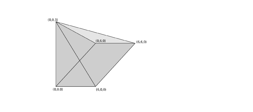
Figure 1: Polytope $Q$.

5 Construction of a surface $X$ of degree $6$ with $45$ handles

Proposition 4.

There exists a real algebraic surface $Y$ of type $(1c)$ such that

$$\mathbb{R}Y\simeq 4S\amalg 2S_{2}\amalg S_{41}.$$

Proof of Theorem 1.

Performing the equivariant deformation described in Proposition 3 to the surface $Y$, we obtain a real sextic surface $X$ in $\mathbb{CP}^{3}$, such that

$$\mathbb{R}X\simeq 4S\amalg 2S_{2}\amalg S_{41}.$$

∎

The rest of the article is devoted to the proof of Proposition 4. Our strategy is first to describe a T-construction of an auxilliary surface $Z$ of Newton polytope $Q$. Then, we use the general Viro’s patchworking method to modify slightly the construction.

5.1 The auxilliary surface $Z$

We describe a triangulation $\tau$ of $Q$ and a distribution of signs $D(\tau)$ at the vertices of $\tau$. Consider the cone $C$ with vertex $(1,0,2)$ over the square $Q_{0}=Q\cap\{w=0\}$ (see Figure 2).

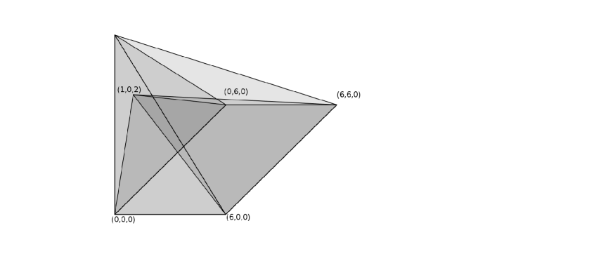
Figure 2: Cone $C$.

Take any primitive convex triangulation of $Q_{0}$ containing the edges depicted in Figure 3.

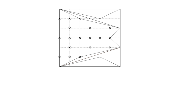
Figure 3: The fixed part of a triangulation of $Q_{0}$ and the distribution of signs. A point gets a sign $+$ if and only if it is ticked.

Then, triangulate $C$ into the cones with vertex $(1,0,2)$ over the triangles of the triangulation of $Q_{0}$. The triangulation of the cone $C$ contains $12$ edges of length $2$ (edges joining $(1,0,2)$ to the points of coordinates $(1,0)\mod 2$ inside $Q_{0}$). For the three edges $[(1,0,2)-(1,0,0)]$, $[(1,0,2)-(3,0,0)]$ and $[(1,0,2)-(5,0,0)]$ of length $2$, refine the triangulation as explained in Definition 9.
Consider the tetrahedra $\alpha_{1}$ and $\alpha_{2}$ with vertices $(1,0,2),(6,6,0),(4,0,1),(6,0,0)$ and $(1,0,2),(0,6,0),(0,0,1),(0,0,0)$ respectively. See Figure 4 for a picture of $\alpha_{1}$.

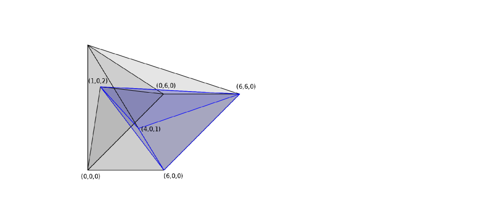
Figure 4: Tetrahedron $\alpha_{1}$.

Triangulate $\alpha_{1}$ into the cones with vertex $(4,0,1)$ over the triangles in the triangulation of the triangle with vertices $(1,0,2),(6,6,0),(6,0,0)$. Triangulate $\alpha_{2}$ into the cones with vertex $(0,0,1)$ over the triangles in the triangulation of the triangle with vertices $(1,0,2),(0,6,0),(0,0,0)$. All the tetrahedra of the triangulations constructed are primitive.
Consider the tetrahedra $\beta_{1}$ and $\beta_{2}$ with vertices $(1,0,2),(6,6,0),(4,4,1),(4,0,1)$ and $(1,0,2),(0,6,0),(0,4,1),(0,0,1)$ respectively. See Figure 5 for a picture of $\beta_{1}$.

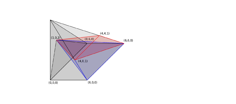
Figure 5: Tetrahedron $\beta_{1}$.

Triangulate $\beta_{1}$ and $\beta_{2}$ into $4$ tetrahedra, respectively, using the subdivision of the segment $[(4,4,1)-(4,0,1)]$ and $[(0,4,1)-(0,0,1)]$ into four primitive edges. All the tetrahedra of the triangulations of $\beta_{1}$ and $\beta_{2}$ are primitive.
Consider the tetrahedron $\gamma_{1}$ with vertices $(1,0,2),(6,6,0),(4,4,1),(0,4,1)$, see Figure 6.

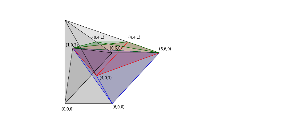
Figure 6: Tetrahedron $\gamma_{1}$.

Triangulate $\gamma_{1}$ into $4$ tetrahedra, using the subdivision of the segment $[(4,4,1)-(0,4,1)]$. All the tetrahedra of the triangulation of $\gamma_{1}$ are of volume $2$.
Consider the tetrahedron $\gamma_{2}$ with vertices $(1,0,2),(6,6,0),(0,6,0),(0,4,1)$. The triangle with vertices $(1,0,2),(6,6,0),(0,6,0)$ is already triangulated. Use this triangulation to subdivise $\gamma_{2}$. Finally, for the three edges $[(1,0,2)-(1,6,0)]$, $[(1,0,2)-(3,6,0)]$ and $[(1,0,2)-(5,6,0)]$ of length $2$, refine the triangulation as explained in Definition 9.
At the present time, the part lying under the cone with vertex $(1,0,2)$ over $Q\cap\{w=1\}$ is triangulated (see Figure 7).

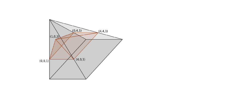
Figure 7: Cone over $Q\cap\{w=1\}$.

Consider the pentagon $P$ with vertices $(1,0,2),(2,0,2),(2,2,2),(1,2,2),(0,1,2)$, triangulate it with any primitive convex triangulation and consider the two cones over it with vertex $(0,0,3)$ and $(4,4,1)$ respectively (see Figure 8).

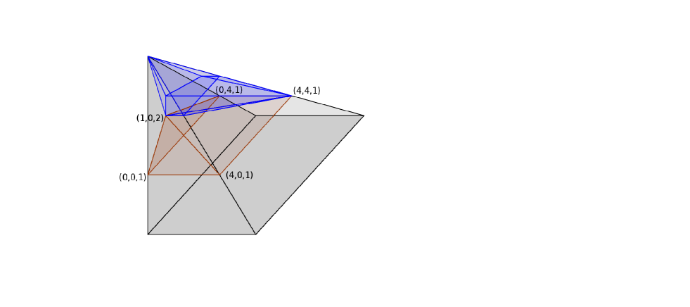
Figure 8: Cones over the pentagon $P$.

Complete the triangulation considering the following tetrahedra:

• The joint of the segment $[(4,0,1)-(4,4,1)]$ and $[(1,0,2)-(2,0,2)]$ triangulated into $4$ primitive tetrahedra, using the triangulation of the segment $[(4,0,1)-(4,4,1)]$ into $4$ edges.

• The joint of the segment $[(0,4,1)-(4,4,1)]$ and $[(0,1,2)-(0,2,2)]$ triangulated into $4$ primitive tetrahedra, using the triangulation of the segment $[(0,4,1)-(4,4,1)]$ into $4$ edges.

• The joint of the segment $[(0,4,1)-(4,4,1)]$ and $[(1,0,2)-(0,1,2)]$ triangulated into $4$ primitive tetrahedra, using the triangulation of the segment $[(0,4,1)-(4,4,1)]$ into $4$ edges.

• The two cones over the triangle $(0,0,2),(1,0,2),(0,1,2)$ with vertices $(0,0,1)$ and $(0,0,3)$, respectively.

• The two cones over the triangle $(0,1,2),(0,2,2),(1,2,2)$ with vertices $(0,4,1)$ and $(0,0,3)$, respectively.

Denote by $\rho$ the obtained subdivision of $Q$. To show the convexity of $\rho$, one can proceed as in  [Ite97]. First, remark that the “coarse” subdivision given by the cone $C$, the tetrahedra $\alpha_{i}$, the tetrahedra $\beta_{i}$, the tetrahedra $\gamma_{i}$, the cones over the pentagon $S$ and the remaining three joints and two cones is convex. Denote by $\nu^{\prime}$ a convex piecewise-linear function certifying the convexity of this “coarse” subdivision.
Choose three convex functions $\nu_{1}$, $\nu_{2}$ and $\nu_{3}$ certifying the convexity of the subdivision of the three edges $\left[(0,0,1)-(0,4,1)\right]$, $\left[(0,4,1)-(4,4,1)\right]$ and $\left[(4,4,1)-(4,0,1)\right]$. Choose also a convex function $\nu_{4}$ certifying the convexity of the chosen subdivision of the pentagon and a convex function $\nu_{5}$ certifying the convexity of the chosen subdivision of the cone $C$.
Consider a piecewise-linear function $\nu:Q\rightarrow\mathbb{R}$ which is affine-linear on each tetrahedron of the subdivision $\rho$ and takes the value $\nu^{\prime}(x)+\sum\epsilon_{i}\nu_{i}(x)$ at every vertex $x$. The function $\nu$ for positive sufficiently small $\epsilon_{i}$ certifies the convexity of the subdivision $\rho$.
Define the distribution of signs $D(\tau)$ at the vertices of $\tau$. For the points inside $Q_{0}$, take the distribution of signs shown in Figure 3. Denote by $A$ a T-curve in $\mathbb{P}^{1}\times\mathbb{P}^{1}$ obtained from the triangulation $\tau$ and the distribution $D(\tau)$ restricted to $Q_{0}$. The chart of $A$ is depicted in Figure 12 b). The distribution of signs at the vertices of $\tau$ belonging to $Q\cap\{w\geq 1\}$ is summarized in Figure 9.

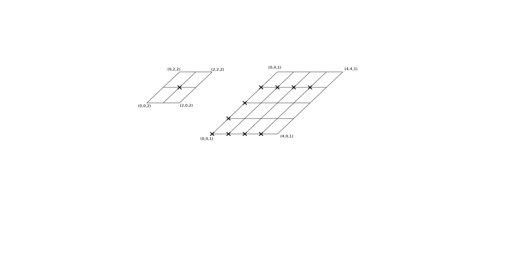
Figure 9: Distibution of signs for $w=1$ and $w=2$. A point gets a sign $+$ if and only if it is ticked.

The point $(0,0,3)$ gets the sign $+$.
Let us compute the Euler characteristic $\chi(\mathbb{R}Z)$ of $\mathbb{R}Z$. The triangulation $\tau$ contains $6$ edges of length $2$ with endpoints of opposite signs, and some tetrahedra of volume $2$ in $\gamma_{1}$ and in the cone $C$. Since all the other tetrahedra are elementary and the stars of the four edges of length $2$ are disjoint, we can use Propositions 1 and 2 to compute $\chi(\mathbb{R}Z)$. In $\gamma_{1}$ all the signs are positive, and in the cone $C$, six tetrahedra of volume $2$ have negative product of signs. One obtains:

$$\chi(\mathbb{R}Z)=\sigma(\mathbb{C}Z)+12=-52.$$

5.2 The surface $Y$

To construct the surface $Y$, we use a real trigonal curve $(C_{3}=0)$ constructed by E. Brugallé in  [Bru06]. The Newton polygon of the polynomial $C_{3}$ is
$Conv((0,0),(6,0),(0,3),(6,1))$ and the chart of $C_{3}$ is depicted in Figure 10.

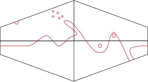
Figure 10: Chart of $(C_{3}=0)$.

Denote by $\Gamma$ the hexagon $Conv((0,0),(4,1),(6,2),(6,4),(4,5),(0,6))$. Consider the charts of the polynomials

• $Y^{3}C_{3}(X,Y)$, $Y^{3}C_{3}(X,\frac{1}{Y})$,

• $Y^{6}b(X^{3}\frac{1}{Y},X^{4}\frac{1}{Y})$, $b(X^{3}Y,X^{4}Y)$,

where $b(X,Y)=Y+(X+x_{1})(X+x_{2})$, with $x_{1},x_{2}>0$ appropriately chosen so that the restrictions of the polynomials $C_{3}(X,Y)$ and $Y^{3}b(X^{3}\frac{1}{Y},X^{4}\frac{1}{Y})$ to $Conv((0,3);(6,1))$ are equal.

Figure 11: Chart of the polynomial P.

By Viro’s patchworking theorem, there exists a polynomial $P$ of Newton polygon $\Gamma$ whose chart is depicted in Figure 11. To construct the surface $Y$, apply the general Viro’s patchworking inside $Q$ with

• the chart of $xz^{2}+P(x,y)$ inside $Conv(\Gamma,(1,0,2))$,

• the same triangulation and distribution of signs as in Section 5.1 outside $Conv(\Gamma,(1,0,2))$.

Denote by $\widehat{A}$ the curve in $\mathbb{P}^{1}\times\mathbb{P}^{1}$ obtained as the intersection of $Y$ with the toric divisor corresponding to the face $Q_{0}$. See Figure 12 a).

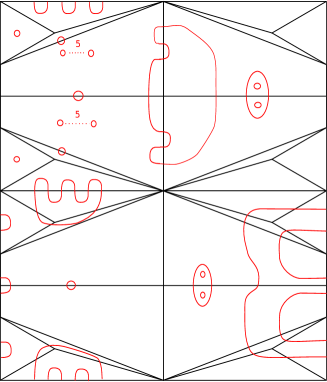
a)

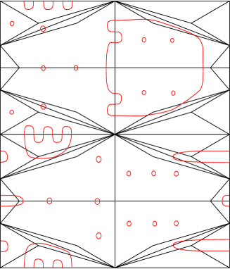
b)

Figure 12: a): $\mathbb{R}\widehat{A}$      b): $\mathbb{R}A$

Let us now compute the Euler caracteristic of $\mathbb{R}Y$. To compute it, we compare the Euler caracteristics of $\mathbb{R}Z$ and $\mathbb{R}Y$. First of all, denote $Z_{1}$ (resp., $Y_{1}$) the surfaces constructed in the same way as $Z$ (resp., $Y$) but where the six edges $[(1,0,2)-(1,0,0)]$, $[(1,0,2)-(3,0,0)]$, $[(1,0,2)-(5,0,0)]$, $[(1,0,2)-(1,6,0)]$, $[(1,0,2)-(3,6,0)]$ and $[(1,0,2)-(5,6,0)]$ are not refined. From Proposition 2, one obtains

$$\chi(\mathbb{R}Y)-\chi(\mathbb{R}Z)=\chi(\mathbb{R}Y_{1})-\chi(\mathbb{R}Z_{1}).$$

Then, notice that outside of $C$, the triangulation and distribution of signs defining $Z_{1}$ and $Y_{1}$ coincide. Denote by $Z_{2}$ (resp., $Y_{2}$) the surfaces with Newton polygon $C$, defined by $(A(x,y)+xz^{2}=0)$ (resp., $(\widehat{A}(x,y)+xz^{2}=0)$) and compactified in $\mathit{Tor}(C)$. These surfaces are singular, with $12$ ordinary double points. However, there exist two homeomorphic compact sets $B\subset\mathbb{R}\mathit{Tor}(Q)$ and $B^{\prime}\subset\mathbb{R}\mathit{Tor}(C)$ such that:

• $\mathbb{R}Y_{1}\setminus B$ is homeomorphic to $\mathbb{R}Z_{1}\setminus B$,

• $\mathbb{R}Y_{2}\setminus B^{\prime}$ is homeomorphic to $\mathbb{R}Z_{2}\setminus B^{\prime}$,

• $\mathbb{R}Y_{1}\cap B$ is homeomorphic to $\mathbb{R}Y_{2}\cap B^{\prime}$,

• $\mathbb{R}Z_{1}\cap B$ is homeomorphic to $\mathbb{R}Z_{2}\cap B^{\prime}$.

So one has:

$$\chi(\mathbb{R}Y_{2}\cap B^{\prime})-\chi(\mathbb{R}Z_{2}\cap B^{\prime})=\chi(\mathbb{R}Y_{1}\cap B)-\chi(\mathbb{R}Z_{1}\cap B).$$

By the additivity of the Euler caracteristic, one also has that

$$\chi(\mathbb{R}Y_{1}\cap B)-\chi(\mathbb{R}Z_{1}\cap B)=\chi(\mathbb{R}Y_{1})-\chi(\mathbb{R}Z_{1}),$$

and

$$\chi(\mathbb{R}Y_{2}\cap B^{\prime})-\chi(\mathbb{R}Z_{2}\cap B^{\prime})=\chi(\mathbb{R}Y_{2})-\chi(\mathbb{R}Z_{2}).$$

So finally

$$\chi(\mathbb{R}Y_{2})-\chi(\mathbb{R}Z_{2})=\chi(\mathbb{R}Y_{1})-\chi(\mathbb{R}Z_{1}).$$

It remains to compute $\chi(\mathbb{R}Y_{2})$ and $\chi(\mathbb{R}Z_{2})$. Topologically, $\mathbb{R}Z_{2}$ is obtained by taking in the quadrant $++$ and $+-$ (resp., $-+$ and $--$) the “double” of $(A\leq 0)$ (resp., $(A\geq 0)$) ramified along $(A=0)\cup(x=0)\cup(x=\infty)$. The same holds for $\mathbb{R}Y_{2}$ by replacing $A$ with $\widehat{A}$, see Figure 13.

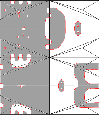
a)

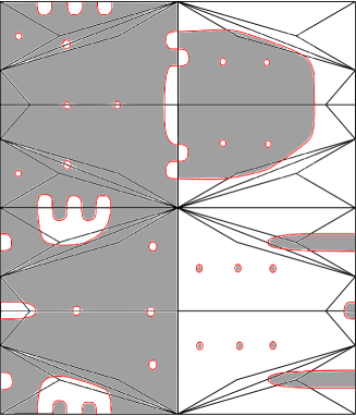
b)

Figure 13: a): $(A(x,y)x<0)$       b): $(\widehat{A}(x,y)x<0)$

By a direct computation, we obtain

$$\chi(\mathbb{R}Y_{2})=2(-18)-12=-48,$$

and

$$\chi(\mathbb{R}Z_{2})=2(-6)-12=-24.$$

Then,

$$\chi(\mathbb{R}Y)-\chi(\mathbb{R}Z)=\chi(\mathbb{R}Y_{2})-\chi(\mathbb{R}Z_{2})=-24.$$

So finally

$$\chi(\mathbb{R}Y)=\chi(\mathbb{R}Z)-24=-52-24=-76.$$

Moreover, $\mathbb{R}Y$ contains two components homeomorphic to $S_{2}$ coming from the double covering of $(\widehat{A}>0)$. Note that the vertices $(1,1,2),(1,3,1),(2,3,1)$ and $(3,3,1)$ have the following property: all the vertices of the triangulation connected to one of these vertices by an edge have the sign $+$, while the vertices $(1,1,2),(1,3,1),(2,3,1)$ and $(3,3,1)$ have the sign $-$. Thus, $\mathbb{R}Y$ contains also four spheres. There is at least one component of $\mathbb{R}Y$ more: this component intersects the plane $\{u=0\}$. Moreover, $\mathbb{R}Y$ cannot have more components, otherwise $Y$ would be an $M$-surface, but $\chi(\mathbb{R}Y)$ does not satisfy the Rokhlin congruence. Finally, from $\chi(\mathbb{R}Y)=-76$, we obtain

$$\mathbb{R}Y\simeq 4S\amalg 2S_{2}\amalg S_{41}.$$

References

- [Bih99] Frédéric Bihan. Une quintique numérique réelle dont le premier nombre de Betti est maximal. C. R. Acad. Sci. Paris Sér. I Math., 329(2):135–140, 1999.
- [Bih01] Frédéric Bihan. Une sextique de l’espace projectif réel avec un grand nombre d’anses. Rev. Mat. Complut., 14(2):439–461, 2001.
- [Bru06] Erwan Brugallé. Real plane algebraic curves with asymptotically maximal number of even ovals. Duke Math. J., 131(3):575–587, 2006.
- [DK00] Alex Degtyarev and Viacheslav Kharlamov. Topological properties of real algebraic varieties: Rokhlin’s way. Uspekhi Mat. Nauk, 55(4(334)):129–212, 2000.
- [Ful98] William Fulton. Intersection theory, volume 2 of Ergebnisse der Mathematik und ihrer Grenzgebiete. 3. Springer-Verlag, Berlin, second edition, 1998.
- [Hor93] Eiji Horikawa. Deformations of sextic surfaces. Topology, 32(4):757–772, 1993.
- [IK96] Ilia Itenberg and Viacheslav Kharlamov. Towards the maximal number of components of a nonsingular surface of degree in . In Topology of real algebraic varieties and related topics, volume 173 of Amer. Math. Soc. Transl. Ser. 2, pages 111–118. Amer. Math. Soc., Providence, RI, 1996.
- [Ite93] Ilia Itenberg. Contre-examples à la conjecture de Ragsdale. C. R. Acad. Sci. Paris Sér. I Math., 317(3):277–282, 1993.
- [Ite97] Ilia Itenberg. Topology of real algebraic -surfaces. Rev. Mat. Univ. Complut. Madrid, 10(Special Issue, suppl.):131–152, 1997. Real algebraic and analytic geometry (Segovia, 1995).
- [Ore01] Stepan Orevkov. Real quintic surface with 23 components. C. R. Acad. Sci. Paris Sér. I Math., 333(2):115–118, 2001.
- [Ris93] Jean-Jacques Risler. Construction d’hypersurfaces réelles (d’après Viro). Astérisque, (216):Exp. No. 763, 3, 69–86, 1993. Séminaire Bourbaki, Vol. 1992/93.
- [Vir80] Oleg Viro. Curves of degree , curves of degree and the Ragsdale conjecture. Dokl. Akad. Nauk SSSR, 254(6):1306–1310, 1980.
- [Vir84] Oleg Viro. Gluing of plane real algebraic curves and constructions of curves of degrees and . In Topology (Leningrad, 1982), volume 1060 of Lecture Notes in Math., pages 187–200. Springer, Berlin, 1984.
- [Wil78] George Wilson. Hilbert’s sixteenth problem. Topology, 17(1):53–73, 1978.