We derive a synaptic weight update rule for learning temporally precise spike train to spike train transformations in multilayer feedforward networks of spiking neurons. The framework, aimed at seamlessly generalizing error backpropagation to the deterministic spiking neuron setting, is based strictly on spike timing and avoids invoking concepts pertaining to spike rates or probabilistic models of spiking. The derivation is founded on two innovations. First, an error functional is proposed that compares the spike train emitted by the output neuron of the network to the desired spike train by way of their putative impact on a virtual postsynaptic neuron. This formulation sidesteps the need for spike alignment and leads to closed form solutions for all quantities of interest. Second, virtual assignment of weights to spikes rather than synapses enables a perturbation analysis of individual spike times and synaptic weights of the output as well as all intermediate neurons in the network, which yields the gradients of the error functional with respect to the said entities. Learning proceeds via a gradient descent mechanism that leverages these quantities. Simulation experiments demonstrate the efficacy of the proposed learning framework. The experiments also highlight asymmetries between synapses on excitatory and inhibitory neurons.

1 Introduction

In many animal sensory pathways, information about external stimuli is encoded in precise patterns of neuronal spikes [1, 2, 3, 4, 5, 6]. If the integrity of this form of information is to be preserved by downstream neurons, they have to respond to these precise patterns of input spikes with appropriate, precise patterns of output spikes. How networks of neurons can learn such spike train to spike train transformations has therefore been a question of significant interest. When the transformation is posited to map mean spike rates to mean spike rates, error backpropagation [7, 8, 9] in multilayer feedforward networks of rate coding model of neurons has long served as the cardinal solution to this learning problem. Our overarching objective in this article is to develop a counterpart for transformations that map precise patterns of input spikes to precise patterns of output spikes in multilayer feedforward networks of deterministic spiking neurons, in an online setting. In particular, we aim to devise a learning rule that is strictly spike timing based, that is, one that does not invoke concepts pertaining to spike rates or probabilistic models of spiking, and that seamlessly generalizes to multiple layers.

In an online setting, the spike train to spike train transformation learning problem can be described as follows. At one’s disposal is a spiking neuron network with adjustable synaptic weights. The external stimulus is assumed to have been mapped—via a fixed mapping—to an input spike train. This input spike train is to be transformed into a desired output spike train using the spiking neuron network. The goal is to derive a synaptic weight update rule that when applied to the neurons in the network, incrementally brings the output spike train of the network into alignment with the desired spike train. With biological plausibility in mind, we also stipulate that the rule not appeal to computations that would be difficult to implement in neuronal hardware. We do not address the issue of what the desired output spike train in response to an input spike train is, and how it is generated. We assume that such a spike train exists, and that the network learning the transformation has access to it. Finally, we do not address the question of whether the network has the intrinsic capacity to implement the input/output mapping; we undertake to learn the mapping without regard to whether or not the network, for some settings of its synaptic weights, can instantiate the input/output transformation. There is, at the current time, little understanding of what transformations feedforward networks of a given depth/size and of a given spiking neuron model can implement, although some initial progress has been made in [10].

2 Background

The spike train to spike train transformation learning problem, as described above, has been a question of active interest for some time. Variants of the problem have been analyzed and significant progress has been achieved over the years.

One of the early results was that of the SpikeProp supervised learning rule [11]. Here a feedforward network of spiking neurons was trained to generate a desired pattern of spikes in the output neurons, in response to an input spike pattern of bounded length. The caveat was that each output neuron was constrained to spike exactly once in the prescribed time window during which the network received the input. The network was trained using gradient descent on an error function that measured the difference between the actual and the desired firing time of each output neuron. Although the rule was subsequently generalized in [12] to accommodate multiple spikes emitted by the output neurons, the error function remained a measure of the difference between the desired and the first emitted spike of each output neuron.

A subsequent advancement was achieved in the Tempotron [13]. Here, the problem was posed in a supervised learning framework where a spiking neuron was tasked to discriminate between two sets of bounded length input spike trains, by generating an output spike in the first case and remaining quiescent in the second. The tempotron learning rule implemented a gradient descent on an error function that measured the amount by which the maximum postsynaptic potential generated in the neuron, during the time the neuron received the input spike train, deviated from its firing threshold. Operating along similar lines and generalizing to multiple desired spike times, the FP learning algorithm [14] set the error function to reflect the earliest absence (presence) of an emitted spike within (outside) a finite tolerance window of each desired spike.

Elsewhere, several authors have applied the Widrow-Hoff learning rule by first converting spike trains into continuous quantities, although the rule’s implicit assumption of linearity of the neuron’s response makes its application to the spiking neuron highly problematic, as explored at length in [14]. For example, the ReSuMe learning rule for a single neuron was proposed in [15] based on a linear-Poisson probabilistic model of the spiking neuron, with the instantaneous output firing rate set as a linear combination of the synaptically weighted instantaneous input firing rates. The output spike train was modeled as a sample draw from a non-homogeneous Poisson process with intensity equal to the variable output rate. The authors then replaced the rates with spike trains. Although the rule was subsequently generalized to multilayer networks in [16], the linearity of the neuron model is once again at odds with the proposed generalization. Likewise, the SPAN learning rule proposed in [17] convolved the spike trains with kernels (essentially, turning them into pseudo-rates) before applying the Widrow-Hoff update rule.

A bird’s eye view brings into focus the common thread that runs through these approaches. In all cases there are three quantities at play: the prevailing error $E(\cdot)$, the output $O$ of the neuron, and the weight $W$ assigned to a synapse. In each case, the authors have found a scalar quantity $\tilde{O}$ that stands-in for the real output spike train $O$: the timing of the only/first spike in [11, 12], the maximum postsynaptic potential/timing of the first erroneous spike in the prescribed window in [13, 14], and the current instantaneous firing rate/pseudo-rate in [15, 16, 17]. This has facilitated the computation of $\partial E/\partial\tilde{O}$ and $\partial\tilde{O}/\partial W$, quantities that are essential to implementing a gradient descent on $E$ with respect to $W$.

Viewed from this perspective, the immediate question becomes why not address $O$ directly instead of its surrogate $\tilde{O}$? After all, $O$ is merely a vector of output spike times. Two major hurdles emerge upon reflection. Firstly, $O$, although a vector, can be potentially unbounded in length. Secondly, letting $O$ be a vector requires that $E(\cdot)$ compare the vector $O$ to the desired vector of spike times, and return a measure of disparity. This can potentially involve aligning the output to the desired spike train which not only makes differentiating $E(\cdot)$ difficult, but also strains biological plausibility [18].

We overcome these issues in stages. We first turn to the neuron model and resolve the first problem. We then propose a closed form differentiable error functional $E(\cdot)$ that circumvents the need to align spikes. Finally, virtual assignment of weights to spikes rather than synapses allows us to conduct a perturbation analysis of individual spike times and synaptic weights of the output as well as all intermediate neurons in the network. We derive the gradients of the error functional with respect to all output and intermediate layer neuron spike times and synaptic weights, and learning proceeds via a gradient descent mechanism that leverages these quantities. The perturbation analysis is of independent interest, in that it can be paired with other suitable differentiable error functionals to devise new learning rules. The overall focus on individual spike times, both in the error functional as well as in the perturbation analysis, has the added benefit that it sidesteps any assumptions of linearity in the neuron model or rate in the spike trains, thereby affording us a learning rule for multilayer networks that is theoretically concordant with the nonlinear dynamics of the spiking neuron.

3 Model of the Neuron

Our approach applies to a general setup where the membrane potential of a neuron can be expressed as a sum of multiple weighted $n$-ary functions of spike times, for varying $n$ (modeling the interactive effects of spikes), where gradients of the said functions can be computed. However, since the solution to the general setup involves the same conceptual underpinnings, for the sake of clarity we use a model of the neuron whose membrane potential function is additively separable (i.e., $n=1$). The Spike Response Model (SRM), introduced in [19], is one such model. Although simple, the SRM has been shown to be fairly versatile and accurate at modeling real biological neurons [20]. The membrane potential, $P$, of the neuron, at the present time is given by

$$P=\sum\limits_{i\in\Gamma}w_{i}\sum\limits_{j\in\mathcal{F}_{i}}\xi_{i}(t^{I}_{i,j}-d_{i})+\sum\limits_{k\in\mathcal{F}}\eta(t^{O}_{k})$$ (1)

where $\Gamma$ is the set of synapses, $w_{i}$ is the weight of synapse $i$, $\xi_{i}$ is the prototypical postsynaptic potential (PSP) elicited by a spike at synapse $i$, $d_{i}$ is the axonal/synaptic delay, $t^{I}_{i,j}-d_{i}$ is the time elapsed since the arrival of the $j^{th}$ most recent afferent (incoming) spike at synapse $i$, and $\mathcal{F}_{i}$ is the potentially infinite set of past spikes at synapse $i$. Likewise, $\eta$ is the prototypical after-hyperpolarizing potential (AHP) elicited by an efferent (outgoing) spike of the neuron, $t^{O}_{k}$ is the time elapsed since the departure of the $k^{th}$ most recent efferent spike, and $\mathcal{F}$ is the potentially infinite set of past efferent spikes of the neuron. The neuron generated a spike whenever $P$ crosses the threshold $\Theta$ from below.

We make two additional assumptions: (i) the neuron has an absolute refractory period that prohibits it from generating consecutive spikes closer than a given bound $r$, and (ii) all input and output spikes that have aged past a given bound $\Upsilon$ have no impact on the present membrane potential of the neuron.

The biological underpinnings of assumption (i) are well known. Assumption (ii) is motivated by the following observations. It is generally accepted that all PSPs and AHPs after an initial rise or fall, decay exponentially fast to the resting potential. This, in conjunction with the existence of an absolute refractory period, implies that for any given $\epsilon$ however small, there exists an $\Upsilon$ such that the sum total effect of all spikes that have aged past $\Upsilon$ can be bounded above by $\epsilon$ (see [21]). Finally, observing that the biological neuron is a finite precision device, we arrive at assumption (ii). The import of the assumptions is that the size of $\mathcal{F}_{i}$ and $\mathcal{F}$ can now be bounded above by $\lceil\Upsilon/r\rceil$. In essence, one has to merely look at a bounded past to compute the present membrane potential of the neuron, and moreover, there are only finitely many efferent and afferent spikes in this bounded past. It helps to conceptualize the state of a network of neurons as depicted in Figure 1(a). The future spike trains generated by the neurons in the network depend only on the future input spikes and the spikes of all neurons in the bounded window $[0,\Upsilon]$.

Figure 1: (a) A feedforward network with two input neurons (shown in black), two intermediate layer neurons (shown in gray) and one output neuron (shown in white). The spike configuration in the bounded time window, $t=0$ (Present) to $t=\Upsilon$ (in the past) is shown. Also shown is the desired output spike train. Note that the desired and the output spike trains differ both in their spike times as well as the number of spikes in the noted time window. (b) The parameterized function $f_{\beta,\tau}(t)$ for various values of $\beta$ and $\tau$. (c) Assigning weights to spikes (denoted by the height of the bars) instead of the corresponding synapse enables a perturbation analysis that derives the effect of a change in the timing or the weight of a spike on the timing of future spikes generated in the network. The weight perturbations are then suitably accumulated at the synapse. The effect of perturbations (marked in magenta) are computed for all input spike weights and intermediate spike times and weights. They are not computed for input spike times since input spike times are given and cannot be perturbed. The effects of the perturbations on other spike times in the configuration space are marked in blue. Note that the blue edges form a directed acyclic graph owing to causality. (d) Simulation data demonstrating that gradient updates can have significant values only immediately after the generation of a spike or the stipulation of a desired spike at the output neuron. Scatter plot of the absolute value of $\frac{\partial E}{\partial t^{O}_{k}}$ in log-scale plotted against $t^{O}_{k}$. The values are drawn from 10,000 randomly generated pairs of vectors ${\mathbf{t}^{O}}$ and ${\mathbf{t}^{D}}$.

We make two other changes. First, we shift the function $\xi_{i}$ to the right so as to include the fixed axonal/synaptic delay. By so doing, we are relieved of making repeated reference to the delay in the analysis. More precisely, what was previously $\xi_{i}(t^{I}_{i,j}-d_{i})$ is now $\xi_{i}(t^{I}_{i,j})$, with the new shifted $\xi_{i}$ satisfying $\xi_{i}(t)=0$ for $t<d_{i}$. The AHP $\eta$ remains as before satisfying $\eta(t)=0$ for $t<0$. Second, and this has major consequences, since our objective is to update the synaptic weights in an online fashion, successive spikes on the same synapse can have potentially different weights (assigned to the spike at its arrival at the synapse). We account for this by assigning weights to spikes rather than synapses; we replace $w_{i}$ by $w_{i,j}$. With these changes in place, we have

$$P=\sum\limits_{i\in\Gamma}\sum\limits_{j\in\mathcal{F}_{i}}w_{i,j}\ \xi_{i}(t^{I}_{i,j})+\sum\limits_{k\in\mathcal{F}}\eta(t^{O}_{k})$$ (2)

4 The Error Functional

Having truncated the output spike train to a finite length vector of spike times, we turn to the error functional. The problem, stated formally, is: given two vectors of spike times, the output spike train $\langle t^{O}_{1},t^{O}_{2},\ldots,t^{O}_{N}\rangle$ and the desired spike train $\langle t^{D}_{1},t^{D}_{2},\ldots,t^{D}_{M}\rangle$ of potentially differing lengths, assign the pair a measure of disparity.

There have been several such measures proposed in the literature (see [23, 24, 25] for details). However, for reasons that we delineate here, these measures do not fit our particular needs well. First and foremost comes the issue of temporal asymmetry. As described earlier, the effect of a spike on the potential of a neuron diminishes with age in the long run, until it ceases altogether at $\Upsilon$. We prefer a measure of disparity that focuses its attention more on the recent than the distant past. If the output and desired spike trains align well in the recent past, this is indicative of the synaptic weights being in the vicinity of their respective desired values. A measure that does not suppress disparity in the distant past will lead weight updates to overshoot. Second comes the issue of the complex relationship between a spike train and its impact on the potential of a neuron, which is the quantity of real interest. We prefer a measure that makes this relationship explicit. Finally comes the issue of the ease with which the measure can be manipulated. We prefer a measure that one can take the gradient of, in closed form. We present a measure that possesses these qualities.

We begin with a parameterized class of non-negative valued functions with shape resembling PSPs.

$$f_{\beta,\tau}(t)=\frac{1}{\tau}e^{\frac{-\beta}{t}}e^{\frac{-t}{\tau}}\quad\textrm{ for}\quad\beta,\tau\geq 0\quad\textrm{ and }\quad t>\epsilon>0$$ (3)

The functions are simplified versions of those in [22]. Figure 1(b) displays these functions for various values of $\beta$ and $\tau$.

We set the putative impact of the vector of output spike times ${\mathbf{t}^{O}}=\langle t^{O}_{1},t^{O}_{2},\ldots,t^{O}_{N}\rangle$ on a virtual postsynaptic neuron to be $\sum_{i=1}^{N}f_{\beta,\tau}(t^{O}_{i})$, and likewise for the vector of desired spike times ${\mathbf{t}^{D}}=\langle t^{D}_{1},t^{D}_{2},\ldots,t^{D}_{M}\rangle$. Our goal is to assess the quantity

$$\left(\sum_{i=1}^{M}f_{\beta,\tau}(t^{D}_{i})-\sum_{i=1}^{N}f_{\beta,\tau}(t^{O}_{i})\right)^{2}$$ (4)

There are two paths we can pursue to eliminate the dependence on the parameters $\beta,\tau$. The first is to set them to particular values. However, reasoning that it is unlikely for a presynaptic neuron to be aware of the shape of the PSPs of its postsynaptic neurons, of which there may be several with differing values of $\beta,\tau$, we follow the second path; we integrate over $\beta$ and $\tau$. Although $\beta$ can be integrated over the range $[0,\infty)$, integrating $\tau$ over the same range results in spikes at $\Upsilon$ having a fixed and finite impact on the membrane potential of the neuron. To regain control over the impact of a spike at $\Upsilon$, we integrate $\tau$ over the range $[0,{\cal T}]$, for a reasonably large ${\cal T}$. By setting $\Upsilon$ to be substantially larger that ${\cal T}$, we can make the impact of a spike at $\Upsilon$ be arbitrarily small. We therefore have:

$$E({\mathbf{t}^{D}},{\mathbf{t}^{O}})=\int_{0}^{\cal T}\int_{0}^{\infty}\left(\sum_{i=1}^{M}f_{\beta,\tau}(t^{D}_{i})-\sum_{i=1}^{N}f_{\beta,\tau}(t^{O}_{i})\right)^{2}d\beta d\tau$$ (5)

Following a series of algebraic manipulations and noting that

$$\int_{0}^{\cal T}\int_{0}^{\infty}\frac{1}{\tau}e^{\frac{-\beta}{t_{1}}}e^{\frac{-t_{1}}{\tau}}\times\frac{1}{\tau}e^{\frac{-\beta}{t_{2}}}e^{\frac{-t_{2}}{\tau}}d\beta d\tau=\frac{t_{1}\times t_{2}}{(t_{1}+t_{2})^{2}}e^{-\frac{t_{1}+t_{2}}{\cal T}}$$ (6)

we get:

$$E({\mathbf{t}^{D}},{\mathbf{t}^{O}})=\sum_{i,j=1}^{M,M}\frac{t^{D}_{i}\times t^{D}_{j}}{(t^{D}_{i}+t^{D}_{j})^{2}}e^{-\frac{t^{D}_{i}+t^{D}_{j}}{\cal T}}+\sum_{i,j=1}^{N,N}\frac{t^{O}_{i}\times t^{O}_{j}}{(t^{O}_{i}+t^{O}_{j})^{2}}e^{-\frac{t^{O}_{i}+t^{O}_{j}}{\cal T}}-2\sum_{i,j=1}^{M,N}\frac{t^{D}_{i}\times t^{O}_{j}}{(t^{D}_{i}+t^{O}_{j})^{2}}e^{-\frac{t^{D}_{i}+t^{O}_{j}}{\cal T}}$$ (7)

$E(\cdot)$ is a bounded from below and achieves its minimum value, 0, at ${\mathbf{t}^{O}}={\mathbf{t}^{D}}$. Computing the gradient of $E(\cdot)$ in Eq 7, we get:

$$\begin{split}&\frac{\partial E}{\partial t^{O}_{i}}=\\ &2\left(\sum_{j=1}^{N}\frac{t^{O}_{j}((t^{O}_{j}-t^{O}_{i})-\frac{t^{O}_{i}}{{\cal T}}(t^{O}_{j}+t^{O}_{i}))}{(t^{O}_{j}+t^{O}_{i})^{3}}e^{-\frac{t^{O}_{j}+t^{O}_{i}}{{\cal T}}}-\sum_{j=1}^{M}\frac{t^{D}_{j}((t^{D}_{j}-t^{O}_{i})-\frac{t^{O}_{i}}{{\cal T}}(t^{D}_{j}+t^{O}_{i}))}{(t^{D}_{j}+t^{O}_{i})^{3}}e^{-\frac{t^{D}_{j}+t^{O}_{i}}{{\cal T}}}\right)\end{split}$$ (8)

5 Perturbation Analysis

We now turn our attention to how perturbations in the weights and times of the input spikes of a neuron translate to perturbations in the times of its output spikes. The following analysis applies to any neuron in the network, be it an output or an intermediate layer neuron. However, we continue to refer to the input and output spike times as $t^{I}_{i,j}$ and $t^{O}_{k}$ to keep the nomenclature simple.

Consider the state of the neuron at the time of the generation of output spike $t^{O}_{l}$. Based on the present spike configuration, we can write

$$\tilde{\Theta}=\sum\limits_{i\in\Gamma}\sum\limits_{j\in\mathcal{F}_{i}}w_{i,j}\ \xi_{i}(t^{I}_{i,j}-t^{O}_{l})+\sum\limits_{k\in\mathcal{F}}\eta(t^{O}_{k}-t^{O}_{l})$$ (9)

Note that following definitions, $\xi_{i}$ returns the value 0 for all $t^{I}_{i,j}<t^{O}_{l}+d_{i}$. Likewise $\eta$ returns the value 0 for all $t^{O}_{k}<t^{O}_{l}$. In other words, we do not have to explicitly exclude input/output spikes that were generated after $t^{O}_{l}$. Note also that we have replaced the threshold $\Theta$ with $\tilde{\Theta}$. This reflects the fact that we are missing the effects of all spikes that at the time of the generation of $t^{O}_{l}$ had values less that $\Upsilon$ but are currently aged beyond that bound. Since these are not quantities that we propose to perturb, their effect on the potential can be considered a constant.

Had the various quantities in Eq 9 been perturbed in the past, we would have

$$\tilde{\Theta}=\sum\limits_{i\in\Gamma}\sum\limits_{j\in\mathcal{F}_{i}}(w_{i,j}+\Delta w_{i,j})\ \xi_{i}(t^{I}_{i,j}+\Delta t^{I}_{i,j}-t^{O}_{l}-\Delta t^{O}_{l})+\sum\limits_{k\in\mathcal{F}}\eta(t^{O}_{k}+\Delta t^{O}_{k}-t^{O}_{l}-\Delta t^{O}_{l})$$ (10)

Combining Eq 9 and Eq 10 and using a first order Taylor approximation, we get:

$$\Delta t^{O}_{l}=\frac{\sum\limits_{i\in\Gamma}\sum\limits_{j\in\mathcal{F}_{i}}\Delta w_{i,j}\xi_{i}(t^{I}_{i,j}-t^{O}_{l})+\sum\limits_{i\in\Gamma}\sum\limits_{j\in\mathcal{F}_{i}}w_{i,j}\frac{\partial\xi_{i}}{\partial t}\!\!\mid_{(t^{I}_{i,j}-t^{O}_{l})}\Delta t^{I}_{i,j}+\sum\limits_{k\in\mathcal{F}}\frac{\partial\eta}{\partial t}\!\!\mid_{(t^{O}_{k}-t^{O}_{l})}\Delta t^{O}_{k}}{\sum\limits_{i\in\Gamma}\sum\limits_{j\in\mathcal{F}_{i}}w_{i,j}\frac{\partial\xi_{i}}{\partial t}\!\!\mid_{(t^{I}_{i,j}-t^{O}_{l})}+\sum\limits_{k\in\mathcal{F}}\frac{\partial\eta}{\partial t}\!\!\mid_{(t^{O}_{k}-t^{O}_{l})}}$$ (11)

We can now derive the final set of quantities of interest from Eq 11:

$$\frac{\partial t^{O}_{l}}{\partial w_{i,j}}=\frac{\xi_{i}(t^{I}_{i,j}-t^{O}_{l})+\sum\limits_{k\in\mathcal{F}}\frac{\partial\eta}{\partial t}\!\!\mid_{(t^{O}_{k}-t^{O}_{l})}\frac{\partial t^{O}_{k}}{\partial w_{i,j}}}{\sum\limits_{i\in\Gamma}\sum\limits_{j\in\mathcal{F}_{i}}w_{i,j}\frac{\partial\xi_{i}}{\partial t}\!\!\mid_{(t^{I}_{i,j}-t^{O}_{l})}+\sum\limits_{k\in\mathcal{F}}\frac{\partial\eta}{\partial t}\!\!\mid_{(t^{O}_{k}-t^{O}_{l})}}$$ (12)

and

$$\frac{\partial t^{O}_{l}}{\partial t^{I}_{i,j}}=\frac{w_{i,j}\frac{\partial\xi_{i}}{\partial t}\!\!\mid_{(t^{I}_{i,j}-t^{O}_{l})}+\sum\limits_{k\in\mathcal{F}}\frac{\partial\eta}{\partial t}\!\!\mid_{(t^{O}_{k}-t^{O}_{l})}\frac{\partial t^{O}_{k}}{\partial t^{I}_{i,j}}}{\sum\limits_{i\in\Gamma}\sum\limits_{j\in\mathcal{F}_{i}}w_{i,j}\frac{\partial\xi_{i}}{\partial t}\!\!\mid_{(t^{I}_{i,j}-t^{O}_{l})}+\sum\limits_{k\in\mathcal{F}}\frac{\partial\eta}{\partial t}\!\!\mid_{(t^{O}_{k}-t^{O}_{l})}}$$ (13)

The first term in the numerator of Eq 12 and Eq 13 corresponds to the direct effect of a perturbation. The second term corresponds to the indirect effect through perturbations in earlier output spikes. The equations are a natural fit for an online framework since the effects on earlier output spikes have previously been computed.

6 Learning via Gradient Descent

We now have all the ingredients necessary to propose a gradient descent based learning mechanism. Stated informally, neurons in all layers update their weights proportional to the negative of the gradient of the error functional. In what follows, we specify the update for an output layer neuron and an intermediate layer neuron that lies one level below the output layer. The generalization to deeper intermediate layer neurons follows along similar lines.

6.1 Synaptic weight update for an output layer neuron

In this case we would like to institute the gradient descent update $w_{i,j}\longleftarrow w_{i,j}-\mu\frac{\partial E}{\partial w_{i,j}}$, where $\mu$ is the learning rate. However, since the $w_{i,j}$’s belong to input spikes in the past, this would require us to reach back into the past to make the necessary change. Instead, we institute a delayed update where the present weight at synapse $i$ is updated to reflect the combined contributions from the finitely many past input spikes in ${\mathcal{F}_{i}}$. Formally,

$$w_{i}\longleftarrow w_{i}-\sum\limits_{j\in\mathcal{F}_{i}}\mu\frac{\partial E}{\partial w_{i,j}}$$ (14)

The updated weight is assigned to the subsequent spike at the time of its arrival at the synapse. $\frac{\partial E}{\partial w_{i,j}}$ is computed using the chain rule (see Figure 1(c)), with the constituent parts drawn from Eq 8 and Eq 12 summed over the finitely many output spikes in ${\mathcal{F}}$:

$$\frac{\partial E}{\partial w_{i,j}}=\sum\limits_{k\in\mathcal{F}}\frac{\partial E}{\partial t^{O}_{k}}\frac{\partial t^{O}_{k}}{\partial w_{i,j}}$$ (15)

6.2 Synaptic weight update for an intermediate layer neuron

The update to a synaptic weight on an intermediate layer neuron follows along identical lines to Eq 14 and Eq 15 with indices $\langle i,j\rangle$ replaced by $\langle g,h\rangle$. The computation of $\frac{\partial t^{O}_{k}}{\partial w_{g,h}}$, the partial derivative of the $k^{th}$ output spike time of the output layer neuron with respect to the weight on the $h^{th}$ input spike on synapse $g$ of the intermediate layer neuron, is as follows. To keep the nomenclature simple, we assume that the $j^{th}$ output spike of the intermediate layer neuron, $t^{H}_{j}=t^{I}_{i,j}$ the $j^{th}$ input spike at the $i^{th}$ synapse of the output layer neuron. Then, applying the chain rule (see Figure 1(c)) we have:

$$\frac{\partial t^{O}_{k}}{\partial w_{g,h}}=\sum\limits_{j\in\mathcal{F}_{i}}\frac{\partial t^{O}_{k}}{\partial t^{I}_{i,j}}\frac{\partial t^{H}_{j}}{\partial w_{g,h}}$$ (16)

with the constituent parts drawn from Eq 13 applied to the output layer neuron and Eq 12 applied to the intermediate layer neuron, summed over the finitely many output spikes of the intermediate layer neuron which are identically the input spikes in ${\mathcal{F}_{i}}$ of the output layer neuron.

6.3 A caveat concerning finite step size

The earlier perturbation analysis is based on the assumption that infinitesimal changes in the synaptic weights or the timing of the afferent spikes of a neuron lead to infinitesimal changes in the timing of its efferent spikes. However, since the gradient descent mechanism described above takes finite, albeit small, steps, caution is warranted for situations where the step taken is inconsistent with the underlying assumption of the infinitesimality of the perturbations. There are two potential scenarios of concern. The first is when a spike is generated somewhere in the network due to the membrane potential just reaching threshold and then retreating. A finite perturbation in the synaptic weight or the timing of an afferent spike can lead to the disappearance of that efferent spike altogether. The perturbation analysis does account for this by causing the denominators in Eq 12 and Eq 13 to tend to zero (hence, causing the gradients to tend to infinity). To avoid large updates, we set an additional parameter that capped the length of the gradient update vector. The second scenario is one where a finite perturbation leads to the appearance of an efferent spike. Since there exists, in principle, an infinitesimal perturbation that does not lead to such an appearance, the perturbation analysis is unaware of this possibility. Overall, these scenarios can cause $E(\cdot)$ to rise slightly at that timestep. However, since these scenarios are only encountered infrequently, the net scheme decreases $E(\cdot)$ in the long run.

7 Experimental Validation

The efficacy of the learning rule derived in the previous section hinges on two factors: the ability of the spike timing based error to steer synaptic weights in the “correct” direction, and the qualitative nature of the nonlinear landscape of spike times as a function of synaptic weights, intrinsic to any multilayer network. We evaluate these in order.

We begin with a brief description of the PSP and AHP functions that were used in the simulation experiments. We chose the PSP $\xi$ and the AHP $\eta$ to have the following forms (see [22] for details):

$$\xi(t)=\frac{1}{\alpha\sqrt{t}}\,e^{\frac{-\beta\alpha^{2}}{t}}\,e^{\frac{-t}{\tau_{1}}}\times\mathcal{H}(t)\qquad\textrm{ and }$$ (17)

$$\eta(t)=-A\,e^{\frac{-t}{\tau_{2}}}\times\mathcal{H}(t)$$ (18)

For the PSP function, $\alpha$ models the distance of the synapse from the soma, $\beta$ determines the rate of rise of the PSP, and $\tau_{1}$ determines how quickly it decays. $\alpha$ and $\beta$ are in dimensionless units. For the AHP function, $A$ models the maximum drop in potential after a spike, and $\tau_{2}$ controls the rate at which the AHP decays. $\mathcal{H}(t)$ denotes the Heaviside step function: $\mathcal{H}(t)=1$ for $t>0$ and $0$ otherwise. All model parameters other than the synaptic weights were held fixed through the experiments. In the vast majority of our experiments, we set $\alpha=1.5$ for an excitatory synapse and $1.2$ for an inhibitory synapse, $\beta=1$, $\tau_{1}=20\,msec$ for an excitatory synapse and $10\,msec$ for an inhibitory synapse. In all experiments, we set $A=1000$ and $\tau_{2}=1.2\,msec$. A synaptic delay $d$ was randomly assigned to each synapse in the range $[0.4,0.9]\,msec$. The absolute refractory period $r$ was set to $1\,msec$ and ${\cal T}$ was set to $150\,msec$. $\Upsilon$ was set to $500\,msec$ which made the impact of a spike at $\Upsilon$ on the energy functional negligible.

7.1 Framework for testing and evaluation

Validating the learning rule would ideally involve presentations of pairs of input/desired output spike trains with the objective being that of learning the transformation in an unspecified feedforward network of spiking neurons. Unfortunately, as observed earlier, the state of our current knowledge regarding what spike train to spike train transformations feedforward networks of particular architectures and neuron models can implement, is decidedly limited. To eliminate this confounding factor, we chose a witness based evaluation framework. Specifically, we first generated a network, with synaptic weights chosen randomly and then fixed, from the class of architecture that we wished to investigate (henceforth called the witness network). We drove the witness network with spike trains generated from a Poisson process and recorded both the precise input spike train and the network’s output spike train. We then asked whether a network of the same architecture, initialized with random synaptic weights, could learn this input/output spike train transformation using the proposed synaptic weight update rule.

We chose a conservative criterion to evaluate the performance of the learning process; we compared the evolving synaptic weights of the neurons of the learning network to the synaptic weights of the corresponding neurons of the witness network. Specifically, the disparity between the synaptic weights of a neuron in the learning network and its corresponding neuron in the witness network was quantified using the mean absolute percentage error (MAPE): the absolute value of the difference between a synaptic weight and the “correct” weight specified by the witness network, normalized by the “correct” weight, averaged over all synapses on that neuron. A MAPE of $1.0$ in the plots corresponds to $100\%$. Note that $100\%$ is the maximum achievable MAPE when the synaptic weights are lower than the “correct” weights.

There are several reasons why this criterion is conservative. Firstly, due to the finiteness of the length of the recorded input/output spike train of the witness network, it is conceivable that there exist other witness networks that map the input to the corresponding output. If the learning network were to tend toward one of these competing witness networks, one would erroneously deduce failure in the learning process. Secondly, turning the problem of learning a spike train to spike train transformation into one of learning the synaptic weights of a network adds a degree of complexity; the quality of the learning process now depends additionally on the characteristics of the input. It is conceivable that learning is slow or fails altogether for one input spike train while it succeeds for another. Notably, the two extreme classes of spike train inputs, weak enough to leave the output neuron quiescent or strong enough to cause the output neuron to spike at its maximal rate, are both noninformative. In spite of these concerns, we found this the most objective and persuasive criterion.

7.2 Time of update

The synaptic weight update rule presented in the previous section does not specify a time of update. In fact, the synaptic weights of the neurons in the network can be updated at any arbitrary sequence of time points. However, as demonstrated here, the specific nature of one of the constituent parts of the rule makes the update insignificantly small outside a particular window of time.

Note that $\frac{\partial E}{\partial t^{O}_{k}}$, the partial derivative of the error with respect to the timing of the $k$th efferent spike of the output neuron, appears in the update formulas of all synapses, be they on the output neuron or the intermediate neurons. We generated 10,000 random samples of pairs of vectors ${\mathbf{t}^{O}}=\langle t^{O}_{1},t^{O}_{2},\ldots,t^{O}_{N}\rangle$ and ${\mathbf{t}^{D}}=\langle t^{D}_{1},t^{D}_{2},\ldots,t^{D}_{M}\rangle$ with $N$ and $M$ chosen independently and randomly from the range $[1,10]$ and the individual spike times chosen randomly from the range $[0,\Upsilon]$. As noted earlier, $\Upsilon$ and ${\cal T}$ were set to $500$ and $150\,msec$, respectively. We computed $\frac{\partial E}{\partial t^{O}_{k}}$ for the individual spikes in each ${\mathbf{t}^{O}}$ according to Eq 8. Figure 1(d) presents a scatter plot in log-scale of the absolute value of $\frac{\partial E}{\partial t^{O}_{k}}$ plotted against $t^{O}_{k}$, for the entire dataset. As is clear from the plot, $|\frac{\partial E}{\partial t^{O}_{k}}|$ drops sharply with $t^{O}_{k}$. Hence, the only time period during which the gradient update formulas can have significant values is when at least one $t^{O}_{k}$ is small, that is, immediately after the generation of a spike by the output neuron. The symmetric nature of Eq 8 would indicate that this is also true for the timing of the desired spikes. We therefore chose to make synaptic updates to the entire network soon after the generation of a spike by the output neuron or the stipulation of a desired spike at the output neuron.

7.3 Efficacy of the error functional – single layer networks

It is clear from Eq 2 that the spike train output of a neuron, given spike train inputs at its various synapses, depends nonlinearly on its synaptic weights. The efficacy of the proposed error functional hinges on how reliably it can steer the synaptic weights of the learning network toward the synaptic weights of the witness network, operating solely on spike time disparities. This is best evaluated in a single layer network (i.e., a single neuron with multiple synapses) since that eliminates the additional confounding nonlinearities introduced by multiple layers.

Consider an update to the synapses of a learning neuron at any point in time. Observe that since the update is based on the pattern of spikes in the finite window $[0,\Upsilon]$, there are therefore uncountably many witness neurons that could have generated that pattern. This class of witness neurons is even larger if there are fewer desired spike times in $[0,\Upsilon]$. A gradient descent update that steers the synaptic weights of the learning neuron in the direction of any one of these potential witness neurons would constitute a “correct” update. It follows that when given a single witness neuron, correctness can only be evaluated over the span of multiple updates to the learning neuron.

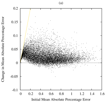
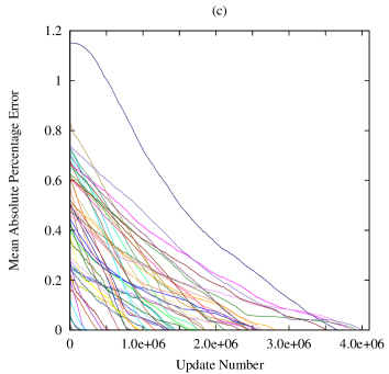
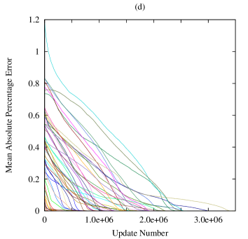
Figure 2: Single neuron with $10$ synapses. (a) and (b) Scatter plot of initial MAPE versus change in MAPE for $10,000$ witness-learning neuron pairs for a bounded number of updates. The neurons in (a) were driven by homogeneous Poisson spike trains and those in (b) by inhomogeneous Poisson spike trains. Points on the yellow lines correspond to learning neurons that converged to their corresponding witness neurons within the bounded number of updates. Note that by definition, points cannot lie above the yellow lines. (c) and (d) $50$ randomly generate witness-learning neuron pairs with learning updates till convergence. Synapses on neurons in (c) are all excitatory and those on neurons in (d) are 80% excitatory and 20% inhibitory. Each curve corresponds to a single neuron. See text for more details regarding each panel.

To obtain a global assessment of the efficacy landscape in its entirety, we randomly generated $10,000$ witness-learning neuron pairs with $10$ excitatory synapses each (the synaptic weights were chosen randomly from a range that made the neurons spike between $5$ and $50$ Hz when driven by a $10$ Hz input) and presented each pair with a randomly generated $10$ Hz Poisson input spike train. Each learning neuron was then subjected to $50,000$ gradient descent updates with the learning rate and cap set at small values. The initial versus change in (that is, initial – final) MAPE disparity between each learning and its corresponding witness neuron is displayed as a scatter plot in Figure 2(a). Across the $10,000$ pairs, $9283$ ($\approx 93\%$) showed improvement in their MAPE disparity. Furthermore, we found a steady improvement of this percentage with increasing number of updates (not shown here). Note that since the input rate was set to be the same across all synapses, a rate based learning model would be expected to show improvement in approximately $50\%$ of the cases.

A closer inspection of those learning neurons that did not show improvement indicated the lack of diversity in the input spike patterns to be the cause. We therefore ran a second set of experiments. Once again, as before, we randomly generated $10,000$ witness-learning neuron pairs. Only this time, input spike trains were drawn from an inhomogeneous Poisson process with the rate set to modulate sinusoidally between $0$ and $10$ Hz at a frequency of $2$ Hz. The modulating rate was phase shifted uniformly for the $10$ synapses. Surprisingly, after just $10,000$ gradient descent updates, $9921$ ($\approx 99\%$) neurons showed improvement, as displayed in Figure 2(b), indicating that with sufficiently diverse input the error functional is globally convergent.

To verify the implications of the above finding with regard to the efficacy landscape, we chose $50$ random witness-learning neuron pairs spread uniformly over the range of initial MAPE disparities, and ran the gradient descent updates until convergence (or divergence). Input spike trains were drawn from the above described inhomogeneous Poisson process. All learning neurons converged to their corresponding witness neurons as displayed in Figure 2(c).

The above experiments indicate that the error functional is globally convergent to the “correct” weights when the synapses on the learning neuron are driven by heterogeneous input. This finding can be related back to the nature of $E(\cdot)$. As observed earlier, Eq 7 makes $E(\cdot)$ nonnegative with the global minima at ${\mathbf{t}^{O}}={\mathbf{t}^{D}}$. For synapses on the learning and witness neuron pair to achieve this for all ${\mathbf{t}^{O}}$ and ${\mathbf{t}^{D}}$, they have to be identical. Furthermore, it follows from Eq 8 that a local minima, if one exists, must satisfy $N$ independent constraints for all ${\mathbf{t}^{O}}$ of length $N$. This is highly unlikely for all ${\mathbf{t}^{O}}$ and ${\mathbf{t}^{D}}$ pairs generated by distinct learning and witness neurons, particularly so if the input spike train that drive these neurons is highly varied. Although, this does not exclude the possibility of the sequence of updates resulting in a recurrent trajectory in the synaptic weight space, the experiments indicate otherwise.

Finally, we conducted additional experiments with neurons that had a mix of excitatory and inhibitory synapses with widely differing PSPs. In each of the $50$ learning-witness neuron pairs, $8$ of the $10$ synapses were set to be excitatory and the rest inhibitory. Furthermore, half of the excitatory synapses were set to $\tau_{1}=80\,msec,\,\beta=5$, and half of the inhibitory synapses were set to $\tau_{1}=100\,msec,\,\beta=50$ (modeling slower NMDA and $\textrm{GABA}_{B}$ synapses, respectively). The results were consistent with the findings of the previous experiments; all learning neurons converged to their corresponding witness neurons as displayed in Figure 2(d).

7.4 Nonlinear landscape of spike times as a function of synaptic weights – multilayer networks

Having confirmed the efficacy of the learning rule for single layer networks, we proceed to the case of multilayer networks. The question before us is whether the spike time disparity based error at the output layer neuron, appropriately propagated back to intermediate layer neurons using the chain rule, has the capacity to steer the synaptic weights of the intermediate layer neurons in the “correct” direction. Since the synaptic weights of any intermediate layer neuron are updated based not on the spike time disparity error computed at its output, but on the error at the output of the output layer neuron, the overall efficacy of the learning rule depends on the nonlinear relationship between synaptic weights of a neuron and output spike times at a downstream neuron.

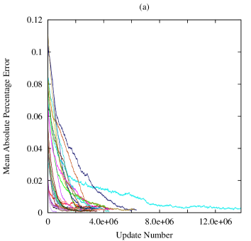
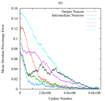
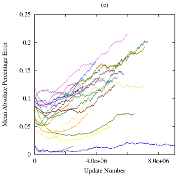
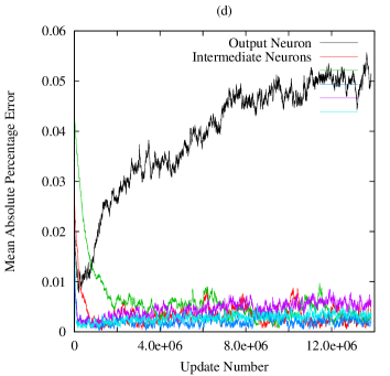
Figure 3: Two layer networks with $30$ synapses ($5$ on each of $5$ intermediate neurons and $5$ on the output neuron). (a) and (c) $50$ randomly generated witness-learning network pairs with learning updates till convergence or divergence. (a) $32$ of the networks converged and (c) the remaining $18$ networks diverged. Each curve corresponds to the average value of the MAPE of the six neurons in the network. (b) and (d) Examples chosen from (a) and (c) respectively showing the MAPE of all six neurons. See text for more details regarding each panel.

We ran a large suite of experiments to assess this relationship. All experiments were conducted on a two layer network architecture with five inputs that drove each of five intermediate neurons which in turn drove an output neuron. There were, accordingly, a sum total of $30$ synapses to train, $25$ on the intermediate neurons and $5$ on the output neuron.

In the first set of experiments, as in earlier cases, we generated $50$ random witness networks with all synapses set to excitatory. For each such witness network we randomly initialized a learning network at various MAPE disparities and trained it using the update rule. Input spike trains were drawn from an inhomogeneous Poisson process with the rate set to modulate sinusoidally between $0$ and $10$ Hz at a frequency of $2$ Hz, with the modulating rate phase shifted uniformly for the $5$ inputs. The most significant insight yielded by the experiments was that the domain of convergence for the weights of the synapses, although fairly large, was not global as in the case of single layer networks. This is not surprising and is akin to what is observed in multilayer networks of sigmoidal neurons. Of the $50$ witness-learning network pairs, $32$ learning networks converged to the correct synaptic weights, while $18$ did not. Figure 3(a) shows the average MAPE disparity (averaged over the 5 intermediate and 1 output neuron) of the $32$ networks that converged to the “correct” synaptic weights. Figure 3(b) shows the MAPE of the six constituent neurons of one of these $32$ networks; each curve in Figure 3(a) corresponds to six such curves.

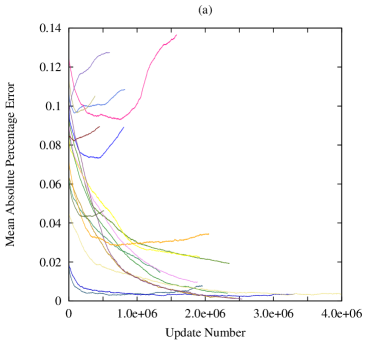
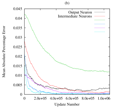
Figure 4: (a) Witness-learning network pairs identical to those in Figure 3(c) driven by new, lower rate, input spike trains. The maximum rate in the inhomogeneous Poisson process was reduced from $10$ to $2$ Hz. The color codes for the specific learning networks are left unchanged to aid visual comparison. (b) The example network in Figure 3(d) driven by the new input spike train. Color codes are once again the same.

Figure 3(c) shows the average MAPE disparity (averaged over the 5 intermediate and 1 output neuron) of the $18$ networks that diverged. A closer inspection of the $18$ networks that failed to converge to the correct synaptic weights indicated a myriad of reasons, not all implying a definitive failure of the learning process. In many cases, all except a few of the $30$ synapses converged. Figure 3(d) shows one such example where all synapses on intermediate neurons as well as three synapses on the output neuron converged to their correct synaptic weights. For synapses on networks that did not converge to the correct weights, the reason was found to be excessively high or low pre/post synaptic spike rates, which as was noted earlier are noninformative for learning purposes (incidentally, high rates accounted for the majority of the failures in the experiments). To elaborate, at high spike rates the tuple of synaptic weights that can generate a given spike train is not unique. Gradient descent therefore cannot identify a specific tuple of synaptic weights to converge to, and consequently the update rule can cause the synaptic weights to drift in an apparently aimless manner, shifting from one target tuple of synaptic weights to another at each update. Not only do the synapses not converge, the error $E(\cdot)$ remains erratic and high through the process. At low spike rates, gradients of $E(\cdot)$ with respect to the synaptic weights drop to negligible values since the synapses in question are not instrumental in the generation of most spikes at the output neuron. Learning at these synapses can then become exceedingly slow.

To corroborate these observations, we ran a second set of experiments on the $18$ witness-learning network pairs that did not converge. We reduced the maximum modulating input spike rate from $10$ to $2$ Hz, i.e., input spike trains were now drawn from an inhomogeneous Poisson process with the rate set to modulate sinusoidally between $0$ and $2$ Hz at a frequency of $2$ Hz. Figure 4(a) shows the average MAPE disparity of the $18$ networks with the color codes for the specific networks left identical to those in Figure 3(c). Only $8$ of the networks diverged this time. Figure 4(b) shows the same network as in Figure 3(d). This time all synapses converged with the exception of one at an intermediate neuron which displayed very slow convergence due to a low spike rate. We chose not to further redress the cases that diverged in this set of experiments with new, tailored, input spike trains to present a fair view of the learning landscape.

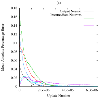
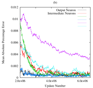
Figure 5: (a) Two layer with $30$ synapses ($5$ on each of $5$ intermediate neurons and $5$ on the output neuron) with two of the inputs and two of the intermediate neurons set to inhibitory. Each curve corresponds to a single neuron. (b) Zoomed view of (a) showing slow convergence. See text for more details regarding each panel.

In our final set of experiments, we explored a network with a mix of excitatory and inhibitory synapses. Specifically, two of the five inputs were set to inhibitory and two of the five intermediate neurons were set to inhibitory. The results of the experiments exhibited a recurring feature: the synapses on the inhibitory intermediate neurons, be they excitatory or inhibitory, converged substantially slower than the other synapses in the network. Figure 5(a) displays an example of a network that converged to the “correct” weights. Note, in particular, that the two inhibitory intermediate neurons were initialized at a lower MAPE disparity as compared to the other intermediate neurons, and that their convergence was slow. The slow convergence is clearer in the the close-up in Figure 5(b). The formal reason behind this asymmetric behavior has to do with the range of values $\frac{\partial t^{O}_{k}}{\partial t^{H}_{j}}$ takes for an inhibitory intermediate neuron as opposed to an excitatory intermediate neuron, and its consequent impact on Eq 16. Observe that $\frac{\partial t^{O}_{k}}{\partial t^{H}_{j}}$, following the appropriately modified Eq 13, depends on the gradient of the PSP elicited by spike $t^{H}_{j}$ at the instant of the generation of spike $t^{O}_{k}$ at the output neuron. The larger the gradient, the greater is the value of $\frac{\partial t^{O}_{k}}{\partial t^{H}_{j}}$. Typical excitatory (inhibitory) PSPs have a short and steep rising (falling) phase followed by a prolonged and gradual falling (rising) phase. Since spikes are generated on the rising phase of inhibitory PSPs, the magnitude of $\frac{\partial t^{O}_{k}}{\partial t^{H}_{j}}$ for an inhibitory intermediate neuron is smaller than that of an excitatory intermediate neuron. A remedy to speed up convergence would be to compensate by scaling inhibitory PSPs to be large and excitatory PSPs to be small, which, incidentally, is consistent with what is found in nature.

8 Discussion

A synaptic weight update mechanism that learns precise spike train to spike train transformations is not only of importance to testing forward models in theoretical neurobiology, it can also one day play a crucial role in the construction of brain machine interfaces. In this article, we have presented such a mechanism formulated with a singular focus on the timing of spikes. The rule is composed of two constituent parts, (a) a differentiable error functional that computes the spike time disparity between the output spike train of a network and the desired spike train, and (b) a suite of perturbation rules that directs the network to make incremental changes to the synaptic weights aimed at reducing this disparity. We have already explored (a), that is, $\frac{\partial E}{\partial t^{O}_{k}}$ as defined in Eq 8, and presented its characteristic nature in Figure 1(d). As regards (b), when the learning network is driven by an input spike train that causes all neurons, intermediate as well as output, to spike at moderate rates, $\frac{\partial t^{O}_{l}}{\partial w_{i,j}}$ as defined in Eq 12 and $\frac{\partial t^{O}_{l}}{\partial t^{I}_{i,j}}$ as defined in Eq 13 can be simplified. Observe that when a neuron spikes at a moderate rate, the past output spike times have a negligible AHP induced impact on the timing of the current spike. Formally stated, $\frac{\partial\eta}{\partial t}$ in Eq 12 and 13 are negligibly small for any output spike train with well spaced spikes. Therefore,

$$\frac{\partial t^{O}_{l}}{\partial w_{i,j}}\approx\frac{\xi_{i}(t^{I}_{i,j}-t^{O}_{l})}{\sum\limits_{i\in\Gamma}\sum\limits_{j\in\mathcal{F}_{i}}w_{i,j}\frac{\partial\xi_{i}}{\partial t}\!\!\mid_{(t^{I}_{i,j}-t^{O}_{l})}}$$ (19)

and

$$\frac{\partial t^{O}_{l}}{\partial t^{I}_{i,j}}\approx\frac{w_{i,j}\frac{\partial\xi_{i}}{\partial t}\!\!\mid_{(t^{I}_{i,j}-t^{O}_{l})}}{\sum\limits_{i\in\Gamma}\sum\limits_{j\in\mathcal{F}_{i}}w_{i,j}\frac{\partial\xi_{i}}{\partial t}\!\!\mid_{(t^{I}_{i,j}-t^{O}_{l})}}$$ (20)

The denominators in the equations above, as in Eq 12 and 13, are normalizing constants that are strictly positive since they correspond to the rate of rise of the membrane potential at the threshold crossing corresponding to spike $t^{O}_{l}$. The numerators relate an interesting story. Although both are causal, the numerator in Eq 20 changes sign across the extrema of the PSP. Accumulated in a chain rule, these make the relationship between the pattern of input and output spikes and the resultant synaptic weight update rather complex.

Our experimental results have demonstrated that feedforward neuronal networks can learn precise spike train to spike train transformations guided by the weakest of supervisory signals, namely, the desired spike train at merely the output neuron. Supervisory signals can of course be stronger, with the desired spike trains of a larger subset of neurons in the network being provided. The learning rule seamlessly generalizes to this scenario with the revised error functional $E(\cdot)$ set as the sum of the errors with respect to each of the supervising spike trains. What is far more intriguing is that the learning rule generalizes to recurrent networks as well. This follows from the observation that whereas neurons in a recurrent network cannot be partially ordered, the spikes of the recurrent network in the bounded window $[0,\Upsilon]$ can be partially ordered according to their causal structure (see Figure 1(c)), which then permits the application of the chain rule. Learning in this scenario, however, seems to be at odds with the sensitive dependence on initial conditions of the dynamics of a large class of recurrent networks [26], and therefore, the issue calls for careful analysis.

References

- [1] Meister, M., Lagnado, L. & Baylor, D.A. (1995) Concerted signaling by retinal ganglion cells. Science 270(5239): 1207-1210.
- [2] deCharms, R.C. & Merzenich, M.M. (1996) Primary cortical representation of sounds by the coordination of action-potential timing. Nature 381(6583): 610-613.
- [3] Neuenschwander, S. & Singer, W. (1996) Long-range synchronization of oscillatory light responses in the cat retina and lateral geniculate nucleus. Nature 379(6567): 728-732.
- [4] Wehr, M. & Laurent, G. (1996) Odour encoding by temporal sequences of firing in oscillating neural assemblies. Nature 384(6605): 162-166.
- [5] Johansson, R.S. & Birznieks, I. (2004) First spikes in ensembles of human tactile afferents code complex spatial fingertip events. Nature Neuroscience 7(2): 170-177.
- [6] Nemenman, I., Lewen, G.D., Bialek, W. & de Ruyter van Steveninck, R.R. (2008) Neural coding of a natural stimulus ensemble: Information at sub-millisecond resolution. PLoS Comp Bio 4, e1000025.
- [7] Bryson, A.E., Ho, Y-C. (1969) Applied optimal control: optimization, estimation, and control. Blaisdell Publishing Company.
- [8] Werbos, P.J. (1974) Beyond Regression: New Tools for Prediction and Analysis in the Behavioral Sciences. PhD thesis, Harvard University.
- [9] Rumelhart, D. E., Hinton, G. E. & Williams, R. J. (1986) Learning representations by back-propagating errors. Nature 323(6088): 533-536.
- [10] Ramaswamy, V. & Banerjee, A. (2014) Connectomic Constraints on Computation in Feedforward Networks of Spiking Neurons. Journal of Computational Neuroscience, 37(2):209-228.
- [11] Bohte, S.M., Kok, J.N., & La Poutre, H. (2002) Error-backpropagation in temporally encoded networks of spiking neurons. Neurocomputing 48(1):17-37.
- [12] Booij, O. & Nguyen, H.t. (2005) A gradient descent rule for spiking neurons emitting multiple spikes. Information Processing Letters 95(6):552-558.
- [13] Gütig, R. & Sompolinsky, H. (2006) The tempotron: a neuron that learns spike timing-based decisions. Nature Neuroscience 9(3):420-428.
- [14] Memmesheimer, R-M., Rubin, R., Olveczky, B. P. & Sompolinsky, H. (2014) Learning Precisely Timed Spikes. Neuron 82:925-938.
- [15] Ponulak, F. & Kasinski, A. (2010) Supervised learning in spiking neural networks with ReSuMe: sequence learning, classification, and spike shifting. Neural Computation 22(2):467-510.
- [16] Sporea, I. & Grüning, A. (2013) Supervised learning in multilayer spiking neural networks. Neural Computation 25(2):473-509.
- [17] Mohemmed, A., Schliebs, S., Matsuda, S., & Kasabov, N. (2012) Span: spike pattern association neuron for learning spatio-temporal spike patterns. Int. J. Neural Syst 22, 1250012.
- [18] Florian, R. V. (2012) The Chronotron: A Neuron That Learns to Fire Temporally Precise Spike Patterns. PLoS ONE 7(8): e40233. doi:10.1371/journal.pone.0040233
- [19] Gerstner, W. (2002) Spiking neuron models: Single neurons, populations, plasticity. Cambridge Univ Press.
- [20] Jolivet, R., Lewis, T.J. & Gerstner, W. (2004) Generalized integrate-and-fire models of neuronal activity approximate spike trains of a detailed model to a high degree of accuracy. Journal of Neurophysiology 92(2):959.
- [21] Banerjee, A. (2001) On the Phase-Space Dynamics of Systems of Spiking Neurons. I: Model and Experiments. Neural Computation 13(1):161-193.
- [22] MacGregor, R.J. & Lewis, E.R. (1977) Neural modeling. Plenum New York.
- [23] Victor, J.D. & Purpura, K.P. (1996) Nature and precision of temporal coding in visual cortex: a metric-space analysis. J Neurophysiol 76:1310–1326.
- [24] van Rossum M.C.W. (2001) A novel spike distance. Neural Computation 13:751–763.
- [25] Schreiber, S., Fellous, J.M., Whitmer, J.H., Tiesinga, P.H.E. & Sejnowski, T.J. (2003). A new correlation based measure of spike timing reliability. Neurocomputing 52:925–931.
- [26] Banerjee A. (2006) On the Sensitive Dependence on Initial Conditions of the Dynamics of Networks of Spiking Neurons. Journal of Computational Neuroscience 20(3):321-348.