Emerging the dark sector from thermodynamics of cosmological systems with constant pressure

Abstract

We investigate the thermodynamics of general fluids that have the constriction that their pressure is constant. For example, this happens in the case of pure dust matter, for which the pressure vanishes and also in the case of standard dark matter phenomenology. Assuming a finite non-zero pressure, the corresponding dynamics is richer than one naively would expect. In particular, it can be considered as a unified description of dark energy and dark matter. We first consider the more general thermodynamic properties of this class of fluids finding the important result that for them adiabatic and isothermal processes should coincide. We therefore study their behaviors in curved space-times where local thermal equilibrium can be appealed. Thus, we show that this dark fluid degenerates with the dark sector of the $\Lambda$CDM model only in the case of adiabatic evolution. We demonstrate that, adding dissipative processes, a phantom behavior can occur and finally we further highlight that an arbitrary decomposition of the dark sector, into ad hoc dark matter and dark energy terms, may give rise to phantom dark energy, whereas the whole dark sector remains non-phantom.

I Introduction

The most accepted cosmological picture suggests that the universe is mostly filled by dark species, which comprise about the $96\%$ of the total energy content CervantesCota:2011pn ; Copeland:2006wr . The dark species are usually decomposed into two fluids: dark matter and dark energy. Dark matter seems to clump at all scales, being responsible for the formation of gravitational potential wells in which baryons fall, forming structures we observe. Conversely, dark energy provides a negative pressure which counteracts the gravitational attraction, accelerating the universe today. The two species, dubbed the universe dark sector, are apparently not related to each other and so one supposes both dark energy and dark matter to be two completely separated constituents. However, there is no unequivocal evidence that the stress-energy tensor of the total dark sector should be split into those two components, leading to a degeneracy problem between cosmological species Kunz:2007rk . Afterwards, there is no reason to assume the dark sector is formed by a single component Hu:1998tj ; Aviles:2011ak ; LUONGO:2014haa ; Xu:2011bp ; Bielefeld:2014gca or by many counterparts, which in principle may also interact Aviles:2011ak . The consequence of this dark degeneracy leads to a plethora of theoretical paradigms, each of them indistinguishable from the standard $\Lambda$CDM model. This degeneracy can be broken, for example, by assuming that dark matter is the clustering component of the dark sector. This serves as a dark matter definition and leaves unsolved the degeneracy problem itself. Indeed, if the dark sector does not interact at all with the particle standard model, it is impossible to disentangle every single dark constituent. Even in presence of interactions, it is not clearly understood how the degeneracy definitively breaks down Aviles:2011ak . An attractive description of the dark sector is obtained by employing one single fluid with vanishing speed of sound Hu:1998tj ; Aviles:2011ak ; LUONGO:2014haa ; Xu:2011bp . This feature ensures fluid perturbations to grow up at all scales Aviles:2011ak and also provides a negative pressure that is responsible for the universe speeding up Aviles:2011ak ; LUONGO:2014haa . This fluid is sometimes also named the dark fluid. One of the advantages of introducing the dark fluid is that dark matter and dark energy are considered as emergent features of a single equation of state (EoS). This is also the underlying philosophy of the generalized Chaplygin gas Kamenshchik:2001cp ; Bento:2002ps ; Bilic:2001cg , which lies on the fundamental advantage that its description can be formulated in terms of scalar fields. Further, it is worth mentioning the Chaplygin gas may also arise from a dark matter viscous fluid Fabris:2005ts , or more generally from purely dissipative effects Zimdahl:2000zm ; Avelino:2008ph ; Li:2009mf ; Avelino:2010pb ; Piattella:2011bs . Coming back to perfect barotropic fluids with vanishing speed of sound, it is easy to notice that their descriptions are equivalent to consider a perfect fluid with constant pressure.

In this paper, we investigate the thermodynamical properties of such a class of fluids. In so doing, we take into account dissipative processes which are typically associated to real fluids. Their introduction is well motivated, due to the fact that generic fluids are usually non-perfect and there exists no robust reasons to characterize the whole dark sector with perfect fluids only. Hence, we depart from thermodynamical equilibrium evolution, by considering either the Eckart Eckart:19403 or causal Muller-Israel-Stewart (MIS) theories Muller1967 ; Israel:1976tn ; Israel:1979wp ; Pavon1982 ; Hiscock:1983zz , showing moreover that our general results do not depend on which approach is employed. Our hypothesis points out to interpret the dark fluid as an approximate description of the dark sector in thermodynamic equilibrium. In our single-fluid approach, both cold dark matter and non-evolving dark energy essentially arise as special cases of zero pressure and zero enthalpy respectively. Thus, we highlight how a standard thermodynamic treatment may open new insights on the study of the dark sector, showing a general landscape to determine its EoS. We are also supported by recent developments on dark energy relativistic thermodynamics which have been investigated both in equilibrium and in the presence of dissipative processes, see e.g. Lima:2004wf ; GonzalezDiaz:2004eu ; Pereira:2008af ; Myung:2009km ; Silva:2011pc ; Aviles:2012et ; Luongo:2012dv ; Silva:2013ixa . Another interesting point is our study on the standard $\Lambda$CDM phenomenology, at equilibrium and out-of-equilibrium, also investigating the role of degeneracy. To do so, we compare evolving dark energy terms at both equilibrium and non-equilibrium stages. For example, if one assumes as evolving dark energy the $w$CDM model, in which the dark energy term is proportional to $(1+z)^{3(1+w)}$, with $w$ a constant EoS parameter, almost all measurements of $w$ are consistent with a non-evolving dark energy Komatsu:2010fb ; Ade:2013zuv ; Chuang:2013wga , nevertheless there is a trend in its expected value to be $w<-1$, leading to phantom dark energy Caldwell:1999ew ; Caldwell:2003vq . Phantom dark energy violates the dominant energy condition Carroll:2003st , and consequently there exist observers measuring a negative energy density. To account this strange behavior, several possibilities occur: one of them lies on accepting the existence of negative energy densities in nature, whereas a second is to abandon the pure $w$CDM model with $w<-1$. A relevant fact is that there exists also the possibility that phantom behavior arises as a dissipative process in the dark energy sector, as shown in Barrow:2004xh ; Cataldo:2005qh ; Cruz:2006ck . It is important to notice that the phantom fluid violates the the dominant energy condition, while a unified fluid does not necessarily violate it. That is why the dark sector decomposition may not exist at all, providing an appealing alternative to the standard cosmological approach. In fact, considering, for example, a unified fluid with EoS $P_{u}=w_{u}\rho_{u}$, and decomposing it as $\rho_{u}=\rho_{ph}+\rho_{dm}$, where ph stands for phantom and $dm$ for dark matter, with EoS parameters $w_{ph}=-\epsilon<-1$ and $w_{dm}=\epsilon\rho_{ph}/\rho_{dm}+w_{u}(\rho_{ph}+\rho_{dm})/\rho_{dm}$, it is evident that the background evolution of both descriptions are the same, without necessarily violating the dominant energy condition. We accurately show this property in the case of our unified dark fluid. For those reasons, one of the main purposes of this article is to investigate thermodynamical systems, leading to the same phenomenology of the $\Lambda$CDM model, but with profound physical departures from it, as out-of-equilibrium processes are involved.

The paper is organized as follows. In Sec. II we review several properties of the dark fluid. In Sec. III we analyze the general properties of a system in thermodynamical equilibrium with constant pressure. In Sec. IV we study the evolution of these systems in a FRW background. In Sec. V we depart from thermodynamical equilibrium by considering the entropy production due to dissipative processes. We study the corresponding universe evolution and we show how out-of-equilibrium processes may lead the dark fluid to become phantom. We also summarize the consequence of first order perturbed equations in the field of cosmological perturbation theory. Finally in Sec. VI we present our conclusions and perspectives.

II The cosmological standard model and the dark fluid

The dark fluid definition may be formulated in terms of either perfect fluids or ideal gases. In the perfect fluid picture, one employs a barotropic EoS providing a vanishing adiabatic speed of sound at all stages of the universe evolution Aviles:2011ak . Since the need of adiabatic perturbations, providing a vanishing sound speed, is not stringent, one can define the barotropic condition even without postulating the EoS at the beginning. The case of perfect gas with vanishing speed of sound LUONGO:2014haa needs no considerations on gravitational instabilities. Indeed, one argues that for barotropic fluids, gravitational instability is driven by the competition between gravitational attraction and pressure. Under the barotropic condition, the zero sound speed allows fluid perturbations to grow at all scales, as cold dark matter actually does. We can write the EoS of a barotropic fluid without losing generality as

$$P_{d}=w_{d}(\rho_{d})\rho_{d}\,,$$ (1)

where the subscript $d$ stands for $dark$. From the restriction of vanishing sound speed, $c^{2}_{s}=dP_{d}/d\rho_{d}=0$, one obtains for the dark fluid

$$w_{d}=\frac{P_{0}}{\rho_{d}}\,,$$ (2)

which implies the pressure to be constant, i.e. $P_{d}=P_{0}$. If the dark fluid is entirely constituted by cold dark matter, the net pressure does not contribute since it is expected to vanish. Astronomical observations, however, do not exclude a priori a non-zero pressure, permitting the existence of a small pressure, even of the order of universe’s critical density today, $\rho_{c}\equiv 3H^{2}_{0}/8\pi G$.

For example, a recent analysis of rotation curves in low surface brightness galaxies has shown that $|w_{dm}|<10^{-6}$ at galaxy centers Barranco:2013wy . This indication enables one to imagine the cosmic speed up to be due to a non-vanishing dark fluid’s pressure. Hence, the possibility that dark energy and dark matter emerge as a single effect due to the dark fluid is plausible. To understand how this is possible, let us consider the continuity equation in a Friedman-Robertson-Walker (FRW) space-time

$$\dot{\rho}_{d}+3\frac{\dot{a}}{a}(\rho_{d}+P_{0})=0\,.$$ (3)

This equation can be integrated to give

$$\rho_{d}(a)=\frac{\rho_{d\,0}}{1+\mathcal{K}}\left(1+\frac{\mathcal{K}}{a^{3}}\right)\,,$$ (4)

where $\mathcal{K}=-(\rho_{d0}+P_{0})/P_{0}$ is an integration constant, fitted considering $\rho_{d0}$ as the value of the dark fluid energy density evaluated at $a(t_{0})\equiv a_{0}=1$. We can notice that Eq. (4) is what one expects for a unified dark sector fluid. It is the sum of a component that decays as $\propto a^{3}$ and a component which remains constant.

To guarantee a positive energy density at all epochs, $\mathcal{K}$ must be positive and therefore the pressure turns out to be negative, lying within the interval $-\rho_{d0}\leq P_{0}\leq 0$. This agrees with current time bounds on cosmic acceleration and allows the dark fluid to accelerate the universe. Eq. (4) definitively forecasts that the dark fluid reproduces the same phenomenology of the $\Lambda$CDM model at the level of background cosmology.

Thereby, the EoS parameter of the dark fluid can be written as

$$w_{d}(a)=-\frac{1}{1+\mathcal{K}a^{-3}},$$ (5)

which may be compared to the $\Lambda$CDM case, consisting of a cosmological constant and cold dark matter contribution

$$w_{\Lambda+\text{dm}}(a)=-\frac{1}{1+\frac{\Omega_{\text{dm}}}{\Omega_{\Lambda}}a^{-3}}\,,$$ (6)

where $\Omega_{\Lambda}=8\pi G\rho_{\Lambda,0}/H_{0}^{2}$. By comparing the two above equations, the correspondence among the two models is attained through the identifications

$$\mathcal{K}=\frac{\Omega_{\text{dm}}}{\Omega_{\Lambda}},\qquad\text{and}\qquad\Omega_{d}=\Omega_{\text{dm}}+\Omega_{\Lambda}\,.$$ (7)

This leads to a degeneracy problem which persists even at linear orders of cosmological perturbation theory. Despite of this degeneracy, we notice an important physical difference between the $\Lambda$CDM and dark fluid paradigms: in the $\Lambda$CDM model to describe the observed late-time acceleration, it is necessary to include the cosmological constant which is commonly reinterpreted as a quantum field vacuum energy contribution. This identification leads to the well-known cosmological constant problem, probably one of the most serious inconsistencies between theoretical physics and observations Weinberg:1988cp . The dark fluid does not suffer from this shortcoming. In fact, in Eq. (4) the term $\mathcal{K}$ does not contain any cosmological information associated to vacuum energy, although the problem to physically motivate $\mathcal{K}$ still persists. In other words, simply assuming that $\mathcal{K}$ is only an integration constant, as obtained integrating the continuity equation, is not enough to physically motivate the dark fluid existence. Hence, the problem belongs to understanding a fundamental theory for the dark fluid which is up to now not completely known, although reasonable advances have been already presented in the literature (see for example Liddle:2006qz ; Reyes:2011ij ). This fundamental theory should motivate $\mathcal{K}$ and the dark fluid itself. In Sec. IV, we provide thermodynamical interpretations of $\mathcal{K}$, able to physically clarify its role in the framework of cosmology and so we propose a self-consistent approach to characterize the dark fluid.

III Thermodynamical systems with constant pressure

We now describe the thermodynamical consequences of systems with constant pressure. Hence, we address a very general thermodynamical scenario, whereas later on, we will use intensive variables to correctly describe the dark fluid phenomenology in the framework of cosmology. In other words, to better understand which consequences occur in the framework of dark fluid’s approach, we first discuss some general features of thermodynamic systems provided with constant pressure. For such systems, the mechanical EoS is restricted to be

$$P=P_{0},$$ (8)

where $P$ is the pressure and $P_{0}$ is a constant. Besides the above hypothesis, we regard the generic thermodynamic system by means of the following extensive variables: the internal (or first-law) energy $U$, from now on simply called the energy, the volume $V$ and the number of constituents, or particles, $N$. Hereafter, we do not distinguish between particles and constituents. We are interested in finding the general properties of this system when the EoS for pressure is restricted to Eq. (8). A thermodynamical system in equilibrium can be completely specified by a fundamental equation, thus we look for a thermodynamical potential from which Eq. (8) may be derived. To this end we work in the entropy representation, the Gibbs equation reads

$$dS=\frac{1}{T}dU+\frac{P}{T}dV-\frac{\mu}{T}dN\,,$$ (9)

where $S(U,V,N)$ is a function of the extensive variables. On the other hand we can write

$$dS=\left(\frac{\partial S}{\partial U}\right)_{V,N}dU+\left(\frac{\partial S}{\partial V}\right)_{U,N}dV+\left(\frac{\partial S}{\partial N}\right)_{U,V}dN\,.$$ (10)

From Eqs. (9) and (10) it follows that a necessary and sufficient condition for guaranteeing the pressure to be constant is

$$\frac{\partial S}{\partial V}-P_{0}\frac{\partial S}{\partial U}=0\,.$$ (11)

Thus, the entropy turns out to be $S(U,V,N)=k_{B}f(U+P_{0}V,N)$. Here, the Boltzmann constant $k_{B}$ is explicitly reported to have the function $f$ dimensionless. Demanding a homogeneous of first degree entropy function, that is, $S(\lambda U,\lambda V,\lambda N)=\lambda S(U,V,N)$, and setting $\lambda=N^{-1}$, we obtain

$$S(U,V,N)=Nk_{B}f\left(\frac{U+P_{0}V}{N}\right)\,.$$ (12)

At this stage, it is helpful to set

$$x\equiv\frac{U+P_{0}V}{N},\qquad F(x)\equiv\frac{df}{dx}\,.$$ (13)

The entropy is therefore drawn up as $S=Nk_{B}f(x)$ and from Eqs. (9) and (10), we obtain the corresponding equations of state

$$\frac{1}{T}=\left(\frac{\partial S}{\partial U}\right)_{V,N}=k_{B}F(x)\,,$$ (14)

$$\frac{P}{T}=\left(\frac{\partial S}{\partial V}\right)_{U,N}=k_{B}P_{0}F(x)\,,$$ (15)

$$\frac{\mu}{T}=-\left(\frac{\partial S}{\partial N}\right)_{U,V}=-k_{B}\big{(}f(x)-xF(x)\big{)}\,.$$ (16)

The case $P=P_{0}$ follows from Eqs. (14) and (15) as expected, whilst the chemical EoS (16) has the form of a Legendre transformation, and as a consequence the Gibbs-Duhem equation, given by

$$d\left(\frac{\mu}{T}\right)=k_{B}xF^{\prime}(x)dx\,,$$ (17)

does not furnish additional thermodynamic information. From Eq. (14), we find that $x$ can be written as a function of the temperature only

$$x=F^{-1}\left(\frac{1}{k_{B}T}\right)\,,$$ (18)

where $F^{-1}$ is the inverse function of $F(x)$. The entropy, written as a function of the temperature $T$, becomes

$$S(P,T,N)=Nk_{B}f\left(F^{-1}\left(\frac{1}{k_{B}T}\right)\right)\,.$$ (19)

For a fixed number of constituents $N$, the entropy becomes a function of the temperature only. In this case, the forthcoming result is that for equilibrium thermodynamical systems with constant pressure isothermal and adiabatic processes coincide.

Moreover, the stability conditions

$$\partial^{2}_{UU}S\leq 0\,,\qquad\partial^{2}_{VV}S\leq 0,\qquad\text{and}\qquad\det S_{,ij}\geq 0\,,$$ (20)

are satisfied for $F^{\prime}(x)<0$.

Cumbersome algebra provides $U(S,V,N)=Nf^{-1}(S/k_{B}N)-P_{0}V$ and $H(S,P,N)=Nf^{-1}(S/k_{B}N)$, where $H$ is the enthalpy, and by using Eq. (19),

$$U(T,V,N)=NF^{-1}\left(\frac{1}{k_{B}T}\right)-P_{0}V\,,$$ (21)

and

$$H(T,P,N)=NF^{-1}\left(\frac{1}{k_{B}T}\right)\equiv Nh(T)\,.$$ (22)

In the last equality we defined the enthalpy per particle $h(T)$. From Eqs. (21) and (22), we find out the heat capacities

$$C_{V}\equiv\left(\frac{\partial U}{\partial T}\right)_{V,N}=-\frac{N}{k_{B}T^{2}}\frac{1}{F^{\prime}(F^{-1}(1/k_{B}T))}\,,$$ (23)

and

$$C_{P}\equiv\left(\frac{\partial H}{\partial T}\right)_{P,N}=C_{V}\,.$$ (24)

From Eq. (23), one infers that $C_{V}\geq 0$ in case $F^{\prime}(x)<0$. Thus, in addition to the condition that entropy is a monotonic growing-function of $U$, and therefore of $x$, if the criterion of stability is appealed, $f(x)$ is naturally convex, i.e. $F(x)>0$ and $F^{\prime}(x)<0$.

A relevant outcome we got is that both heat capacities coincide, whereas the adiabatic index is $\gamma\equiv C_{P}/C_{V}=1$, as expected since the pressure is constant.

By using Eq. (21), we obtain for the energy density $\rho\equiv U/V$

$$\rho=-P_{0}+\frac{Nh(T)}{V}\,.$$ (25)

Above we demonstrated that, albeit we involved an adiabatic expansion, the temperature is a constant. It follows that for a positive energy density, for arbitrary ratios $V/N$, the condition

$$P_{0}<0\,,$$ (26)

must hold. The pressure of the system is a negative constant quantity as a consequence of the thermodynamics here presented.

The case of negative pressure is not unusual in nature. Examples of systems in which this condition holds are given in Wheeler:Nature ; Coupin:bib ; Stanley:2002281 and references therein. In those examples, the particular choices of thermodynamic conditions naturally portray the fact that the pressure is negative.

Another example is derived from Geometrothermodynamics Quevedo:2006xk . This formalism has been proposed to describe thermodynamical system on pure geometrical grounds. Geometrothermodynamics also provides a way to obtain fundamental equations as solutions of an extremal surfaces principle Vazquez:2011ia . The cosmological consequences of one of such solutions have been studied in Aviles:2012et , leading to an extension of the generalized Chaplygin gas, which for some specific choice of their free parameters reduces to a dark fluid with entropy

$$S=S_{0}N\ln\left(\frac{U+cV}{N}\right),$$ (27)

which is of the form of Eq. (12), and consequently the pressure becomes constant. Using the above formalism, we obtain the entropy of the system as a function of the temperature $S(T,N)=S_{0}N\ln(S_{0}T)$. Note that this entropy results unbounded from below, thus the Nerst postulate is violated in this particular example. The resulting energy density is

$$\rho=-P_{0}+\frac{NS_{0}T}{V}\,,$$ (28)

which, if compared to Eq. (25), provides $h(T)=S_{0}T$.

III.1 The emergent cosmological constant

In the case of zero constant pressure, the system described by Eq. (25), gives as density a direct functional dependence in terms of the volume and temperature as:

$$\rho=\frac{Nh(T)}{V}.$$ (29)

One recognizes that the former represents the case of dust particles if the system is maintained at constant temperature. Here, the dark fluid reduces to a pure dark matter component. This would be also the case of non-interacting baryonic particles.

Obtaining a pure dark energy term is subtler. It corresponds to the particular case in which the enthalpy vanishes, i.e.

$$h(T)=F^{-1}\left(\frac{1}{k_{B}T}\right)=0\,.$$ (30)

Generally, the above equality is valid at one specific temperature, hereafter $T_{\Lambda}$. Inverting the equation to get $T_{\Lambda}$, one gets

$$T_{\Lambda}=\frac{1}{k_{B}F(x)|_{x=0}}\,,$$ (31)

implying at $x=0$, $U=-P_{0}V$, or equivalently

$$\rho=-P_{0}\,.$$ (32)

Immediately, we can notice that if the temperature takes the constant value $T_{\Lambda}$, any adiabatic processes maintain the same temperature at all stages of the universe evolution, providing an overall both adiabatic and isothermal process. However, it is clear that any deviation from equilibrium increases the entropy. Due to this fact a corresponding temperature change is expected. In this situation, Eq. (30) is no longer satisfied, and we therefore refer to pure dark energy as a unstable fine-tuning case.

IV Intensive variables and background Cosmology

A complete and general picture accounting thermodynamics in curved space-time has not definitively forecasted. Before proposing an approach able to describe such a situation, it is convenient to reobtain all results of Sec. III by means of intensive variables, which show the advantage to be locally defined. We thus define the specific entropy (per particle), $\sigma\equiv S/N$, and the particle density $n\equiv N/V$. The entropy therefore reads

$$\sigma=k_{B}f(x)\,,$$ (33)

and its variation in terms of first order differential form

$$d\sigma=k_{B}F(x)dx\,,$$ (34)

where now $x=(\rho+P_{0})n^{-1}$. Using Eqs. (18) and (23) above, it follows:

$$d\sigma=\frac{c_{V}(T)}{T}dT\,,$$ (35)

where $c_{V}(T)\equiv C_{V}(T,N)/N$ is the specific heat capacity (per particle) at constant volume, with its definition given by Eq. (23) —Analogous definition for $c_{P}(T)$ will be used below. In this case we derived from local variables the result that the entropy is a function of the temperature only. The corresponding Gibbs equation (9) becomes

$$Td\sigma=\frac{1}{n}\left[d\rho-\frac{\rho+P}{n}dn\right]\,,$$ (36)

or, altenatively,

$$Td\sigma=\frac{1}{n}\left(\frac{\partial\rho}{\partial T}\right)_{n}dT+\frac{1}{n}\left[\left(\frac{\partial\rho}{\partial n}\right)_{T}-\frac{\rho+P}{n}\right]dn\,.$$ (37)

By comparing Eqs. (35) and (37) we obtain

$$\rho=-P_{0}+h(T)n\,,$$ (38)

which confirms Eq. (25). Consequences on background cosmology are easily accounted by appealing local thermodynamical equilibrium. To do so, let us divide the whole system at fixed FRW-coordinate time $t$ in spatial cell subsystems each with comoving volume $V_{0}$ and constituent number $N$, wherein local equilibrium holds. In this picture, the processes are considered quasi-static and the thermodynamic equilibrium is recovered at every stage of local evolution, although a whole equilibrium is not necessarily addressed. The corresponding physical volume $V$ is related to the scale factor, becoming $V(a)=V_{0}(a/a_{0})^{3}$, and then we obtain, for the energy density evolution

$$\rho(a)=\frac{\rho_{0}}{1+\mathcal{K}_{0}}\left(1+\frac{\mathcal{K}(T,N)}{a^{3}}\right)\,.$$ (39)

where $\mathcal{K}$ is a function of $T$ and $N$

$$\mathcal{K}(T,N)=-\frac{1}{P_{0}}Nh(T)\frac{a^{3}_{0}}{V_{0}}\equiv-v^{-1}\frac{h(T)}{P_{0}}\,,$$ (40)

Notice in the last equality we defined the specific comoving volume per constituent, $v\equiv V_{0}/a_{0}^{3}N$, and $\mathcal{K}_{0}\equiv\mathcal{K}(a_{0})$. Soon, it is evident that Eq. (39) generalizes Eq. (4), in which non-adiabatic contributions have been included through the term $\mathcal{K}(T,N)$.

In case of constant $N$, we choose $V_{0}$ such that $v=1$ and we absorb the volume units in the definition of $h(T)$, simplifying our notation. Further, in the absence of bulk viscosity, the universe expansion history follows an adiabatic local equilibrium process, otherwise the symmetries of homogeneity and isotropy would break, as we will demonstrate in Sec. V. We showed in Sec. III that adiabatic processes are also isothermal for a system with constant pressure. Thus, the enthalpy per particle becomes a constant as well, $h(T)=h(T_{0})$, and

$$\mathcal{K}=-\frac{h(T_{0})}{P_{0}}\,.$$ (41)

Hence, for an adiabatic process, with a fixed number of constituents $N$, $\mathcal{K}$ is a constant equal to the enthalpy over the pressure, contained in a unitary comoving volume, recovering Eq. (4). A relevant consequence of our formalism is that $\mathcal{K}$ is no longer an integration constant, since it was derived from thermodynamical first principles. This may be reviewed as a first explanation of its physical meaning, permitting to better justify the dark fluid existence.

Using Eqs. (7), a comparison with the $\Lambda$CDM model gives

$$h(T_{0}) = \rho_{c}\Omega_{\text{dm}},$$ (42)

$$P_{0} = \rho_{c}\Omega_{\Lambda},$$ (43)

In the absence of a thermodynamical fundamental equation, we cannot invert Eq. (42) to obtain the value of $T_{0}$. However, we could appeal to several possible considerations on how to treat both the dark fluid and “visible” sector. The first possibility is to assume that the dark fluid and the “visible” sector had a common thermal origin. Afterwards, they decoupled at a precise energy scale, $k_{B}T_{*}$, thereafter the temperature of the dark fluid was maintained constant by an adiabatic expansion and today its value is $T_{0}=T_{*}$. In this scenario, the decoupling era had to be at very early times, so that $a-a_{*}\simeq a$, where $a_{*}$ is the decoupling scale factor and $a$ lies on the range considered throughout this article. A second approach is that no interactions between the dark and “visible” sectors were present at all. Thus, $T_{*}$ becomes the temperature at which our description starts to be valid, whereas $a_{*}$ the corresponding scale factor. Moreover, since the $\Lambda$CDM has been probed to match data, especially at early times by cosmic microwave background observations, we also conclude that $a_{*}\rightarrow 0$. Both approaches provide that the time $t_{*}$, defined by $a_{*}=a(t_{*})$, is very small. The only difference is that, in the first scenario the temperature $T_{*}$ is very large and is considered as a freezing temperature $T_{*}>\mathcal{O}(\text{MeV})/k_{B}$ (above the primordial nucleosynthesis scale), while in the second case its value is not constrained by these considerations.

Afterwards, we extend the framework of constant pressure, enabling it to vary. In an adiabatic process, it can be shown that the following relation holds Weinberg:1971mx :

$$\left(\frac{\partial\rho}{\partial T}\right)_{n}\frac{\dot{T}}{T}=\left(\frac{\partial P}{\partial T}\right)_{n}\frac{\dot{n}}{n}\,.$$ (44)

In the case of constant pressure, the right hand side of Eq. (44) vanishes and we obtain again that the temperature is a constant. We note that the same happens for a baryonic dust component and the well-known relation, $T_{b}\propto a^{-2}$, is naturally recovered if we consider the kinetic theory of non-relativistic particles. The artificial EoS, $P_{dust}=0$, although a good approximation, led us to a non-sense conclusion providing a constant dust temperature. We can reach analogous results for the case of constant pressure. If we naively extrapolate the above ideas to the case of the dark fluid, we may simply set $P=P_{0}+nkT$, and $\rho=n(m+3kT/2)$, obtaining again $T\propto a^{-2}$. However, this approach lies on kinetic theory considerations, which may not apply for the dark fluid case.

V Entropy production

In this section, we investigate out-of-equilibrium processes enabling the dark fluid to deviate from its standard evolution, which degenerates with the $\Lambda$CDM model. First, since a complete description of the dark fluid is so far unknown, we develop an alternative approach and we summarize some interesting points, which will be helpful when we discuss entropy production generated by out-of-equilibrium processes. Let us assume that the constant pressure shifts to $P_{*}=P_{0}+\pi$. The effect of the dynamical pressure $P_{*}$ is to induce a temperature change given by

$$\frac{\dot{T}}{T}=\left(\frac{\partial\pi}{\partial\rho}\right)_{n}\frac{\dot{n}}{n}\,,$$ (45)

obtaining that the temperature is no longer a constant. The term $\pi$ is named bulk viscosity, in the context of dissipative processes of irreversible thermodynamics. In such a case, Eq. (44) is no longer valid because of the corresponding entropy production. In Sec. V, we will see that Eq. (45) holds only for the case in which $\pi(T,n)$ is a linear function of $T$. In this situation, we may assume $\pi=\pi_{0}(n)+\pi_{1}(n)T$, and with the aid of Eq. (24), we find that Eq. (45) becomes

$$\frac{c_{P}(T)dT}{T}=\frac{\pi_{1}(n)\,dn}{n^{2}}\,.$$ (46)

In relativistic Eckart’s theory Eckart:19403 , $\pi_{1}$ is negative, and assuming the number density decays with universe’s expansion, we obtain the well-known result that viscosity is capable of raising the fluid temperature. To properly introduce the out-of-equilibrium processes, it is convenient to split the stress-energy tensor in a piece that correspond to equilibrium states plus a piece that contains the dissipative terms as

$$T^{\mu\nu}=T^{\mu\nu}_{equi}+D^{\mu\nu}\,.$$ (47)

It is always possible to choose a four vector velocity field $u^{\mu}$ for which the energy density $\rho$ and the particle density number $n$ coincide with their equilibrium values Eckart:19403 ; Weinberg:1971mx , dealing with the commonly named N-frame. We decompose $T^{\mu\nu}$ in proper components of $u^{\mu}$, giving

$$T^{\mu\nu}_{equi}=\rho u^{\mu}u^{\nu}+Ph^{\mu\nu}\,,$$ (48)

$$D^{\mu\nu}=\pi h^{\mu\nu}+q^{\mu}u^{\nu}+q^{\nu}u^{\mu}+\pi^{\mu\nu}\,,$$ (49)

where

$$h_{\mu\nu}=g_{\mu\nu}+u_{\mu}u_{\nu}\,,$$ (50)

is the projector tensor on spatial hypersurfaces normal to $u^{\mu}$ and

$$\pi=\frac{1}{3}h_{\mu\nu}D^{\mu\nu}\,,$$ (51)

$$\pi^{\mu\nu}=D^{\langle\mu\nu\rangle}\equiv\frac{1}{2}h^{\mu}_{\,\,\alpha}h^{\nu}_{\,\,\beta}\left(D^{\alpha\beta}+D^{\beta\alpha}\right)-\frac{1}{3}h_{\alpha\beta}D^{\alpha\beta}h^{\mu\nu}\,,$$ (52)

$$q^{\nu}=-u^{\alpha}h^{\beta\nu}D_{\alpha\beta}\,,$$ (53)

are the dissipative terms, which can be identified with bulk viscosity, shear viscosity and heat flow, respectively. Thus,

$$q^{\nu}u_{\nu}=\pi^{\mu\nu}u_{\nu}=\pi^{\alpha}_{\,\,\alpha}=0,\qquad h^{\nu}_{\,\,\alpha}q^{\alpha}=q^{\nu},\qquad h^{\mu}_{\,\,\alpha}\pi^{\alpha\nu}=\pi^{\mu\nu},\qquad\pi^{\mu\nu}=\pi^{\langle\mu\nu\rangle}\,.$$ (54)

From the conservation equations $\nabla_{\mu}T^{\mu\alpha}=0$, we obtain by contracting with $u_{\alpha}$, the continuity equation

$$\dot{\rho}+\Theta\big{(}\rho+P+\pi\big{)}+\big{(}\nabla_{\mu}+\dot{u}_{\mu}\big{)}q^{\mu}+\pi^{\mu\nu}\sigma_{\mu\nu}=0\,,$$ (55)

and by contracting with $h^{\nu}_{\,\,\alpha}$ the three hydrodynamical Euler equations

$$h^{\mu\nu}\nabla_{\mu}\big{(}P+\pi\big{)}+\big{(}\rho+P+\pi\big{)}\dot{u}^{\nu}+h^{\nu}_{\,\,\alpha}\dot{q}^{\alpha}+\left(\frac{4}{3}\Theta h^{\nu}_{\,\,\alpha}+\sigma^{\nu}_{\,\,\alpha}+\omega^{\nu}_{\,\,\alpha}\right)q^{\alpha}+h^{\nu}_{\,\,\alpha}\nabla_{\mu}\pi^{\mu\alpha}=0\,.$$ (56)

The dot over an arbitrary tensor is the covariant derivative along the integral curves of $u^{\mu}$ ($\dot{\mathbf{A}}\equiv u^{\mu}\nabla_{\mu}\mathbf{A}$); additionally $\Theta=\nabla_{\mu}u^{\mu}$, $\sigma_{\mu\nu}=\nabla_{\langle\nu}u_{\mu\rangle}$, $\omega_{\alpha\beta}=h^{\mu}_{\,\,\alpha}h^{\nu}_{\,\,\beta}\nabla_{[\nu}u_{\mu]}$ are the expansion scalar, the shear and the vorticity of the world lines defined by $u^{\mu}$, respectively.

In this N-frame, the particle density flux is

$$n^{\mu}=nu^{\mu}\,,$$ (57)

therefore, the conservation of particle density flux $\nabla_{\mu}n^{\mu}=0$ gives

$$\dot{n}+\Theta n=0\,.$$ (58)

In local equilibrium, the entropy flux is given by

$$S^{\mu}_{equil}=n\sigma u^{\mu}\,,$$ (59)

thus, the entropy density is given by $-u_{\mu}S^{\mu}_{equil}=n\sigma$. Further, out-of-equilibrium, the entropy flux vector becomes

$$S^{\mu}=n\sigma u^{\mu}+\frac{q^{\mu}}{T}-Q^{\mu}(\pi,q^{\alpha},\pi^{\alpha\beta};u^{\alpha})\,,$$ (60)

where $Q^{\mu}$ is the most general function quadratic in the dissipative terms and $\sigma$ is the equilibrium specific entropy. The Eckart theory lies on neglecting $Q^{\mu}$, although this leads to instantaneous propagation of heat Israel:1976tn and undesired instabilities in the system Hiscock:1983zz . The introduction of $Q^{\mu}$ is necessary to account for those effects apart from the case where gradients of $\pi$, $q^{\alpha}$ and $\pi^{\mu\nu}$ are negligible Maartens:1996vi . By the Gibbs equation (36) and the continuity equation (55), the rate of change of the entropy per particle is

$$nT\dot{\sigma}=-\pi\Theta-\big{(}\nabla_{\mu}+\dot{u}_{\mu}\big{)}q^{\mu}-\pi^{\mu\nu}\sigma_{\mu\nu}\,,$$ (61)

and the entropy flux becomes

$$T\nabla_{\mu}S^{\mu}=-\pi\Theta-\left(\frac{\partial_{\mu}T}{T}+\dot{u}_{\mu}\right)q^{\mu}-\pi^{\mu\nu}\sigma_{\mu\nu}-T\nabla_{\mu}Q^{\mu}\,.$$ (62)

In relativistic thermodynamics the second law of thermodynamics is written as an inequality on the divergence of the entropy flux Eckart:19403 ; Weinberg:1971mx ; Misner:1974qy

$$\nabla_{\mu}S^{\mu}\geq 0\,,$$ (63)

that is, the rate at which the entropy is generated can either vanish or be positive Misner:1974qy .

V.1 The temperature rate of change

Now, let us consider the rate of change along integral curves of $u^{\mu}$ of the energy density $\rho(n,T)$,

$$\dot{\rho}=\left(\frac{\partial\rho}{\partial n}\right)_{T}\dot{n}+\left(\frac{\partial\rho}{\partial T}\right)_{n}\dot{T}.$$ (64)

Using the identity

$$\left(\frac{\partial P}{\partial T}\right)_{n}\dot{T}=\rho+P-n\left(\frac{\partial\rho}{\partial T}\right)_{n},$$ (65)

and the Gibbs equation, we obtain for the rate change of the temperature

$$\left(\frac{\partial\rho}{\partial T}\right)_{n}\frac{\dot{T}}{T}=n\dot{\sigma}+\left(\frac{\partial P}{\partial T}\right)_{n}\frac{\dot{n}}{n}.$$ (66)

Using now Eq. (61)

$$\left(\frac{\partial\rho}{\partial T}\right)_{n}\dot{T}=-\pi\Theta-\big{(}\nabla_{\mu}+\dot{u}_{\mu}\big{)}q^{\mu}-\pi^{\mu\nu}\sigma_{\mu\nu}+T\left(\frac{\partial P}{\partial T}\right)_{n}\frac{\dot{n}}{n}.$$ (67)

So far, the analysis performed in Eq. (67) is general, and hence, applies for any fluid described by the stress-energy tensor (47). Further, one can notice that Eq. (45) is recovered when $\pi$ is a linear function of the temperature. Therefore, the effect of bulk viscosity is not to shift the pressure from $P$ to $P+\pi$ only, but also it affects the temperature rate change differently from the pressure, as showed in Eq. (67). Applying this result to the case of constant pressure, and having $(\partial\rho/\partial T)_{n}=nc_{v}(T)=nc_{p}(T)$, Eq. (67) then reduces to

$$nc_{p}(T)\dot{T}=-\pi\Theta-\big{(}\nabla_{\mu}+\dot{u}_{\mu}\big{)}q^{\mu}-\pi^{\mu\nu}\sigma_{\mu\nu}.$$ (68)

V.2 The case of background Cosmology and phantom behavior

Now, let us consider the effect of the dissipative terms in a spatial homogeneous and isotropic universe. We write the FRW spatially flat metric as

$$ds^{2}=-dt^{2}+a^{2}(t)\delta_{ij}dx^{i}dx^{j}\,.$$ (69)

The time coordinate $t$ coincides with the proper time of the free fall observers comoving with the Hubble flow. In these coordinates, the four velocity is written as $u^{\mu}=(1,{\bf 0})$, and a dot over a scalar quantity becomes the partial derivative with respect to $t$, e.g. for a scalar function $f$, $\dot{f}=\partial_{t}f$.

The only dissipative term, compatible with this geometry is the bulk viscosity, thus Eq. (61) becomes

$$\dot{\sigma}=-\frac{\pi\Theta}{nT}\,,$$ (70)

and the Gibbs equation leads to

$$nT\dot{\sigma}=-\pi\Theta=\dot{\rho}+\Theta(\rho+P)\,.$$ (71)

Since we are considering a FRW metric the expansion scalar is $\Theta=3H=3\dot{a}/a$, and appealing conservation of particle flux (see Eq. (58) above) we obtain $n=n_{0}a^{3}_{0}/a^{3}$. By Eq. (68) the temperature change is

$$c_{p}(T)\dot{T}=-\frac{\pi\Theta}{n}=-3a^{2}\dot{a}\pi\,.$$ (72)

Soon, we notice that the second law of thermodynamics requires

$$\nabla_{\mu}S^{\mu}=n\dot{\sigma}-\nabla_{\mu}Q^{\mu}(\pi^{2};u^{\alpha})\geq 0\,.$$ (73)

In Eckart’s theory, the quadratic term $Q^{\mu}$ is neglected and customarily one can choose the algebraical equation

$$\pi=-3H\zeta\,,$$ (74)

with $\zeta>0$, which reduces to the Newtonian Stokes law $\pi=-\zeta\vec{\nabla}\cdot\vec{v}$ in the non relativistic limit, and ensures the positivity of the entropy flux divergence. Thereafter, $\zeta=\zeta(\rho)=\rho^{-1/2}g(\rho)$, thus if non-dark components are neglected, $\rho^{-1/2}H$ is a constant and $\pi$ becomes a function of the energy density only. This is equivalent to simply choose $\pi=\pi(a)$ in a manner that the condition (73) is satisfied. Thus, anagously, in Eckart’s theory, we could simply set $\pi=\pi(a)<0$ as well. However, if early time evolution is considered, we cannot neglect the “visible” sources and $\rho^{-1/2}H$ is no longer constant. A particular remark is that several authors prefer to give a dependence $\zeta=\zeta(\rho_{total})$, where $\rho_{total}$ is the total energy density, implying interactions among the dark and “visible” sectors. In so doing, the dependence of $\pi$ on $H$ can be avoided.

In the following, we adopt the general approach in which the bulk viscosity $\pi$ is a function of $\rho$ and $H$, or a function of $a$ and $\dot{a}$,

$$\pi=\pi(a,\dot{a})\,.$$ (75)

In MIS causal theory, $Q^{\mu}$ is not neglected and being quadratic in the bulk viscosity one arrives to

$$\nabla_{\mu}S^{\mu}=-\frac{\pi}{T}\left[3H+\beta_{0}\dot{\pi}+\frac{1}{2}T\nabla_{\alpha}\left(\frac{\beta_{0}}{T}u^{\alpha}\right)\pi\right]\,,$$ (76)

where $\beta_{0}$ is a phenomenological non-negative coefficient —it is the coefficient of the $\pi^{2}$ term in $Q^{\mu}$. The simplest way to satisfy the second law of thermodynamics is to impose

$$\tau_{0}\dot{\pi}+\pi=-3\zeta H-\left[\frac{1}{2}\zeta T\nabla_{\alpha}\left(\frac{\beta_{0}}{T}u^{\alpha}\right)\pi\right]\,,$$ (77)

which is obtained by equating the terms inside the brackets of Eq. (76) to $-\pi$, and the $\zeta$ and $\tau_{0}$ coefficients are related among them by $\beta_{0}=\tau_{0}/\zeta$, having the meaning of bulk viscosity strength and relaxation time, respectively. This first order differential equation is well supported by arguments derived from the standard kinetic theory Israel1976213 , which does not necessarily have to apply to the dark fluid.

In kinetic theory $\tau_{0}$ is identified with the mean free path of the particles, and if $\tau_{0}\ll H$, Eq. (77) reduces to Maartens:1996vi

$$\tau_{0}\dot{\pi}+\pi=-3\zeta H\,.$$ (78)

This equation is the transport equation in the truncated MIS theory for bulk viscosity. Given the two phenomenological functions $\zeta$ and $\tau_{0}$ we can solve for $\pi$ and $\rho$. Alternatively we can adopt a phenomenological $\pi=\pi(a,\dot{a})$ and Eq. (77) (or Eq. (78)) becomes a constriction on $\zeta$ and $\tau_{0}$.

Now, giving $dh=c_{p}(T)dT$ for constant pressure systems, we obtain from Eq. (72) the enthalpy change

$$\dot{h}=-3a^{2}\pi(a,\dot{a})\dot{a}\,.$$ (79)

Our main goal is to find out a general solution $h=h(a)$. Unfortunately, this is impossible for the general case of Eq. (75) by using only Eq. (79), we thus have to integrate the complete system of equations, that is, the Friedmann equation

$$H^{2}=\frac{8\pi G}{3}\rho_{total}\,,$$ (80)

the continuity equation (55), which we appropriately rewrite as

$$\dot{\rho_{d}}+3H(\rho_{d}+P_{0}+\pi)=0\,,$$ (81)

and the corresponding continuity equations for the non-dark components. To close the system we need the equation for the bulk viscosity, which is generally chosen to be one of (74), (77) or (78) for Eckart, MIS or truncated MIS, respectively. Nevertheless, we emphasize that those restrictions, although well motivated for standard non-dark fluids, are not strictly necessarily, they are just the easiest way to ensure the positivity of the entropy flux divergence.

In the special case where $\pi$ is a function of the scale factor only, $\pi=\pi(a)$, Eq. (79) can be integrated, from the very beginning, obtaining

$$h(a)=h(a_{*})-3\int_{a_{*}}^{a}a^{\prime}{}^{2}\pi(a^{\prime})da^{\prime}\,,$$ (82)

where $a_{*}=a(T_{*})$ and following the considerations given in Sec. IV, $a_{*}$ must be the value of the scale factor at a very early time. Using now Eq. (38), we get

$$\rho(a)=-P_{0}-\frac{3}{a^{3}}\int_{a_{*}}^{a}a^{\prime}{}^{2}\pi(a^{\prime})da^{\prime}+\frac{h(a_{*})}{a^{3}}.$$ (83)

The energy change, due to dissipative bulk viscosity, gets the attractive form $\Delta U=-\pi(V)\Delta V$. Although Eq. (82) is an exact solution for the case $\pi=\pi(a)$, the general case obeys the same relation once we found the solution $\pi(a)=\pi(a,\dot{a}(a))$. Given the freedom on $\zeta$ and $\tau_{0}$ as functions of $\rho$ in Eqs. (74), (77) or (78), there are uncountable different forms that the bulk viscosity can take. This enables to follow a phenomenological approach by employing a particular dependence $\pi(a)$, which thereafter could be naively compared with observations.

As a first example of this approach, let us consider the case in which $\pi$ is solved as a power-law function of the scale factor,

$$\pi=\pi_{0}a^{\epsilon},$$ (84)

where $\epsilon$ and $\pi_{0}<0$ are real constants. The contribution to the energy density $\rho_{diss}$, due to dissipative quantities, becomes then

$$\rho_{diss}=\frac{3|\pi_{0}|}{\epsilon+3}a^{\epsilon},\qquad(\epsilon\neq-3)$$ (85)

where we consider $a-a_{*}\simeq a$.

As a result, in the case $\epsilon>0$, we find that $\rho_{diss}$ leads to a phantom behavior. Thus, we may consider a time $t_{i}$ for which we neglect all contributions to the energy density except the dissipative quantities. It is therefore straightforward to show that the scale factor will blow up to infinity in a finite time given by:

$$t_{BigRip}=t_{i}+\frac{\epsilon+3}{8\pi G|\pi_{0}|\epsilon a_{i}^{\epsilon/2}}\,,$$ (86)

where $a_{i}\equiv a(t_{i})$, corresponding to a Big Rip Caldwell:2003vq (see also Astashenok:2012iy ; Pavon:2012pt ).

A second interesting example shows up a Little Rip behavior Frampton:2011sp ; Brevik:2011mm ; Frampton:2011rh ; Astashenok:2012tv . In our formalism this can be achieved, for example, by considering the function

$$\pi(a)=-|\pi_{0}|ae^{-a/a_{P}}\,,$$ (87)

where $a_{P}$ is a given scale. Using Eqs. (83) and (87), or by directly integrating Eq. (81), we obtain the energy density

$$\rho(a)=-P_{0}+\frac{h(a_{*})}{a^{3}}+\rho_{diss}\,,$$ (88)

where

$$\rho_{diss}=\frac{18|\pi_{0}|a_{P}^{4}}{a^{3}}-3|\pi_{0}|a_{p}e^{-a/a_{P}}\Big{[}1+3\frac{a_{P}}{a}+6\left(\frac{a_{P}}{a}\right)^{2}+6\left(\frac{a_{P}}{a}\right)^{3}\Big{]}\,,$$ (89)

is the term induced by the dissipative viscosity of the dark fluid, in which again we have considered $a-a_{*}\simeq a$. Further, we define the effective EoS parameter $w_{*}$ as

$$w_{*}=\frac{-P_{0}+\pi(a)}{\rho}\,.$$ (90)

In Fig. 1 we show the evolution of the energy density of the dissipative dark fluid and its EoS parameter. We note that although $w_{*}<-1$ in a given interval of the scale factor, it tends towards $-1$ as the scale factor grows, leading to a Little Rip solution. In this same interval we note that the energy density is a growing function of the scale factor. As a reference, we also show the energy density of the dark fluid without dissipatives and its EoS parameter. Both models are adjusted so that their present abundances are $\Omega_{d}=0.96$.

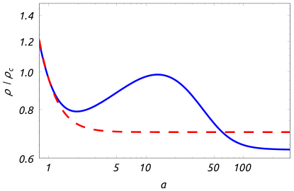
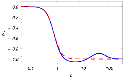
Figure 1: Evolution of the little rip model expressed by Eq. (87) (solid curves) and of the dark fluid (dashed curves). Left panel: Energy density in units of the critical energy density nowadays as a function of the scale factor. Right panel: Effective EoS parameter as a function of the scale factor. Here $a_{P}=10$ and $|\pi_{0}|=0.1\rho_{c}$.

V.3 The arbitrary decomposition and phantom behavior

In Sec. I, we emphasized that the phantom behavior occurs when decomposing the dark sector into two species. In this section we show explicitly how this may occur in our formalism.

We decompose the dark fluid including dissipative terms in dark energy and dark matter contributions, as $\rho=\rho_{de}+\rho_{dm}$, with

$$\rho_{dm}=\frac{h(a_{*})}{a^{3}}\,,$$ (91)

$$\rho_{de}=-P_{0}+\frac{3}{a^{3}}\int^{a}_{a_{*}}a^{\prime}{}^{2}\pi(a^{\prime})da^{\prime}\,.$$ (92)

Rephrasing it differently, we are interpreting the consequences of the out-of-equilibrium processes as a dark energy effect. The condition for having a phantom dark energy is $\rho_{de}+P_{0}+\pi<0$, or alternatively

$$a^{3}\pi(a)-3\int^{a}_{a_{*}}a^{\prime}{}^{2}\pi(a^{\prime})da^{\prime}<0\,,$$ (93)

while the condition for the total dark fluid to be non-phantom is $\rho_{dm}+\rho_{de}+P_{0}+\pi>0$, or

$$h(a_{*})+a^{3}\pi(a)-3\int^{a}_{a_{*}}a^{\prime}{}^{2}\pi(a^{\prime})da^{\prime}\geq 0\,,$$ (94)

and leads also to a non-phantom dark energy. We can join those two conditions into a single one, having:

$$0<3\int^{a}_{a_{*}}a^{\prime}{}^{2}\pi(a^{\prime})da^{\prime}-a^{3}\pi(a)\leq h(a_{*})\,,$$ (95)

which is equivalent to $0<-(\rho_{de}+P_{0}+\pi)<\rho_{dm}$.

Thus, if dark fluid’s dissipative effects accomplish the above inequality, we easily get that the decomposition into dark matter and dark energy provides a phantom dark energy contribution. This violates the dominant energy condition, whereas the dark fluid, as a whole, behaves non-phantom. As a simple example, we consider a constant $\pi_{0}$, the inequality (95) holds if $0<-a^{3}_{*}\pi_{0}<h(a_{*})$. This particular example also shows that we may obtain the dark energy contribution from a pure dark matter fluid, i.e. $P_{0}=0$, with dissipative processes.

A more interesting example arises from the bulk viscosity defined in Eq. (87). We can decompose the whole dark fluid as $\rho_{d}=\rho_{de}+\rho_{dm}$, with $\rho_{de}=-P_{0}+\rho_{diss}$ ($\rho_{diss}$ has been given by Eq. (89)) and $\rho_{dm}=h(a_{*})/a^{3}$. For small values of the bulk viscosity strength $|\pi_{0}|$, the total energy density $\rho_{d}$ does not become a growing function of the scale factor (contrary to the situation in Fig. 1). In the left panel of Fig. 2, we show such a behavior, choosing $a_{P}=10$ and $|\pi_{0}|=0.001\rho_{c}$. The solid curve corresponds to the dark fluid energy density. We soon note that $d\rho_{d}/da\leq 0$ in its whole domain, while the arbitrary dark energy component, plotted with a dot-dashed curve, shows up a phantom behavior for $a\lesssim a_{P}$. It is worthly to note that Eq. (95) is accomplished in the interval where $d\rho_{de}/da\geq 0$. In the right panel of Fig. 2 we show the evolution of the scale factor, the solid (blue) line corresponds to the this case, and we note that $H(a)$ is not growing, while the case $|\pi_{0}|=0.1\rho_{c}$, depicted with a dotted (orange) line is.

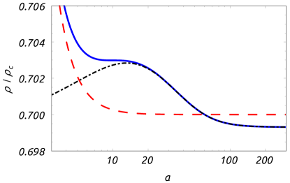
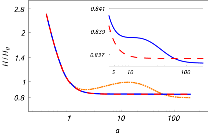
Figure 2: (Color online) Evolution for the little rip model expressed by Eq. (87). Left panel: Evolution of the energy density, the dot-dashed curve shows the $\rho_{de}$ contribution and the solid curve (blue) the total dark fluid energy density. We note that, while the dark energy contribution is phantom in some region, the total dark fluid is not. Here $a_{P}=10$ and $|\pi_{0}|=0.001\rho_{c}$. The long-dashed curve (red) shows the evolution of the dark fluid energy density without dissipatives. Right panel: Evolution of the Hubble factor. The dotted (orange) curve is for the model with $|\pi_{0}|=0.1$, corresponding to the case of Fig. 1, the other two curves as in the left panel. The inset shows a zoom to the region for which the differences between the cases of dark fluid with and without dissipatives are evident. We notice that for a viscosity strenght $|\pi_{0}|=0.1\rho_{c}$ there is a region for which $dH/da>0$, while for viscosity strenght $|\pi_{0}|=0.001\rho_{c}$ there is not.

V.4 Dissipative processes in cosmological perturbations

In this subsection, we give a brief description of the behavior of perturbations in the presence of dissipative processes. To this end, we write the metric of the perturbed universe for scalar perturbations in the Newtonian-conformal gauge as

$$ds^{2}=a^{2}(\tau)\big{[}-(1+2\Psi)d\tau^{2}+(1-2\Phi)\delta_{ij}dx^{i}dx^{j}\,\big{]}.$$ (96)

The potentials $\Psi$ and $\Phi$ are the usual metric scalar perturbations, which are related to the Poisson equation and to the geodesic equations respectively. We introduced the conformal time $\tau$ which, in the absence of perturbations, it is related to the cosmic time $t$ by $dt=a(\tau)d\tau$. Using these coordinates the four-velocity becomes

$$u^{\mu}=\frac{1}{a}\big{(}1-\Psi,v^{i}\big{)},$$ (97)

where $v^{i}$ is the peculiar velocity, i.e., the average velocity the particles have with respect to the Hubble flow.

In the coordinates described by Eq. (96), the stress-energy tensor components become

$$T^{0}{}_{0} = -\bar{\rho}(1+\delta)\,,$$ (98)

$$T^{0}{}_{i} = (1+w^{*})\bar{\rho}v_{i}+\frac{1}{a}q_{i}\,,$$ (99)

$$T^{i}{}_{j} = (\bar{P}+\delta P+\pi+\delta\pi)\delta^{i}_{j}+\pi^{i}_{\,\,j}\,.$$ (100)

Note that $\bar{\rho}$, $\bar{P}$ and $\pi$ are background quantities which only depend on the time coordinate $\tau$, whereas $\rho=\bar{\rho}+\delta\rho=\bar{\rho}(1+\delta)$, $P=\bar{P}+\delta P$ are respectively the total energy density and isotropic pressure of the fluid. The fluid expansion scalar becomes

$$\Theta=\frac{1}{a}\Big{(}3\mathcal{H}(1-\Psi)+\partial_{i}v^{i}-3\dot{\Phi}\Big{)},$$ (101)

and the shear viscosity is

$$\sigma_{ij}=\frac{1}{2}a(\partial_{i}v_{j}+\partial_{j}v_{i})-\frac{1}{3}a\partial_{k}v^{k}\delta_{ij}.$$ (102)

We note that the vorticity does not appear in the linear perturbed equations, because it is multiplied in Eq. (56) by the heat transfer, which is also a perturbed quantity. It is convenient to define $v_{q}^{i}$ through the components of the heat transfer $q^{\mu}$ as

$$q^{\mu}=\frac{(1+w^{*})\bar{\rho}}{a}(0,v^{i}_{q}).$$ (103)

With this definition the indices of $v_{q}^{i}$ (as well as for $v^{i}$) are raised and lowered through the euclidian metric $\delta_{ij}$. After some manipulations of Eqs. (55) and (56), we rearrange the continuity equation

$$\partial_{\tau}\delta+(1+w^{*})\left(\theta^{*}-3\partial_{\tau}\Phi\right)+3\mathcal{H}\left(\frac{\delta P^{*}}{\delta\rho}-w^{*}\right)\delta=0,$$ (104)

and the Euler equation

$$\partial_{\tau}\theta^{*}+\mathcal{H}(1-3w^{*})\theta^{*}+\frac{\partial_{\tau}w^{*}}{1+w^{*}}\theta^{*}-k^{2}\frac{\delta P^{*}/\delta\rho}{1+w^{*}}\delta-k^{2}\Psi+k^{2}\pi_{s}=0\,,$$ (105)

which have been conventionally reported in the Fourier space. We also defined

$$\theta^{*}\equiv\theta+\theta_{q}\,,$$ (106)

where as usual $\theta\equiv\partial_{i}v^{i}$, and analogously: $\theta_{q}\equiv\partial_{i}v^{i}_{q}$. We also get the shear viscosity scalar

$$\pi_{s}\equiv-\frac{k_{i}k^{j}\pi^{i}_{\,j}}{k^{2}(1+w^{*})\bar{\rho}}=\frac{4\eta\theta}{3a(1+w^{*})\bar{\rho}}.$$ (107)

(Note that contrary to $k^{i}$, $\pi_{ij}$ are components of a tensor.) As usual, we chose the shear viscosity to satisfy $\pi_{\mu\nu}=-2\eta\sigma_{\mu\nu}$, ensuring that the entropy flux grows as it can be seen in Eq. (60). We notice that apart from the scalar shear viscosity in Eq. (105), the continuity and Euler equations are the same of a perfect fluid with pressure $P_{*}=P_{0}+\pi$. We further require the use of Einstein’s equations, which give

$$k^{2}\Phi=-4\pi Ga^{2}\rho\Delta^{*},\qquad\text{where}\qquad\Delta^{*}\equiv\delta+3\mathcal{H}(1+w^{*})\frac{\theta^{*}}{k^{2}},$$ (108)

and

$$k^{2}(\Phi-\Psi)=16\pi Ga^{2}\,\eta\frac{\theta}{a},$$ (109)

where we perform a sum also over other non-dark fluid contributions to the right hand side of the above equations. Immediately, a relevant consequence arises: if shear viscosity is here neglected, this set of equations does not allow one to distinguish heat transfer from dark fluid’s velocity divergence. Rephrasing it differently, one gets that only bulk viscosity can be constrained by linear perturbation theory. However, this opens the possibility to use observations of the visible matter velocities, at non-linear orders, in order to isolate $\theta$ from $\theta_{*}$, gaining valuable information on dark fluid’s heat transfer. This treatment is beyond the aims of this paper, but will be object of future investigations. In the following, we therefore neglect shear viscosity and solve the perturbed system in the presence of bulk viscosity. For completeness, we consider as specific model the one given by Eq. (87) with $a_{P}=10$ and $|\pi_{0}|=0.001\rho_{c}$. Given these values, the dark fluid is non-phantom and $1+w_{*}>0$ at all stages of its evolution. In so doing, the Euler equation, as reported in Eq. (105), is also well defined. To obtain the perturbation of the viscosity $\pi(a)$, we make use of the substitution $a\rightarrow a(1+\Psi)$, having

$$\delta\pi=\frac{a}{a_{P}}|\pi_{0}|(a-a_{P})e^{-a/a_{P}}\Psi.$$

We may describe the evolutions of Eqs. (104), (105), (108), and the corresponding continuity and Euler equations for baryons. To do so, we notice that the differences with the $\Lambda$CDM model arise only at late times. At that epoch, we neglect the contribution of radiation and we start the evolution at redshifts circumscribed after the recombination.

In Figs. 3 we show the differences between the model with viscosity and the pure dark fluid. We plot the differences

$$\frac{\Delta\delta_{b}}{\delta_{b}}=\frac{\delta_{b}-\delta_{b}^{(fid)}}{\delta_{b}},\qquad\frac{\Delta\phi_{b}}{\phi_{b}}=\frac{\phi_{b}-\phi_{b}^{(fid)}}{\phi_{b}},$$

where the label $fid$ refers to as the fiducial dark fluid without dissipative terms (degenerated with the $\Lambda$CDM model).

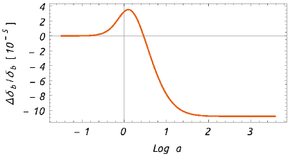
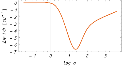
Figure 3: Perturbation evolutions of the little rip model, defined in Eq. (87), evolving as a function of the scale factor logarithm. In particular, in the left panel we plot the differences in the evolution of the energy density contrast of baryonic matter, while in the right panel we plot the difference in the evolution of the Newtonian potential $\Phi$.

VI Final outlooks and perspectives

In this work, we investigated the thermodynamical properties of a class of fluids whose corresponding pressure is a non-zero constant. In the context of cosmology this restriction gives rise to a unified dark energy fluid, for which both dark energy and dark matter emerge as a single effect. This dark fluid hypothesis lies on the assumption that the involved fluid is barotropic and provides a vanishing speed of sound. The latter property allows perturbations to grow at all scales and at the same time provides a constant negative pressure that accelerates the universe. Previous investigations on the dark fluid were mainly based on assuming the validity of the continuity equation, valid for pure adiabatic processes. Consequently, the characteristic scale $\mathcal{K}$ would represent an integration constant, as here showed, and cannot be physically well-supported in order to describe the difference between the dark fluid and the standard $\Lambda$CDM model. In this paper, we studied the dark fluid properties in a more general thermodynamical context. We therefore showed that its evolution generally differs from the one associated to the standard $\Lambda$CDM model. In particular, we found that $\mathcal{K}$ is no longer an integration constant, becoming instead a function of the temperature, described by the ratio of fluid’s enthalpy and pressure contained in a unitary co-moving volume. The consequences in cosmology are relevant. First, we demonstrated that, for constant pressure systems, adiabatic and isothermal processes should coincide, and therefore the dark fluid and the $\Lambda$CDM models degenerated in the case of adiabatic expansions only. Given that fluids are generally non-perfect, we expected that dissipative processes arose, leading to an important breaking of the above mentioned degeneracy between the standard model and the dark fluid itself. Thus, we treated the case of bulk viscosity in detail at the background and perturbed cosmological levels and we also considered to introduce the shear viscosity and heat transfer. We followed a phenomenological approach and from the beginning we gave a dependence on the scale factor to the bulk viscosity. Our treatment deeply departures from either Eckart’s or MIS theories. Afterwards, we explicitly showed that our working scheme is somehow equivalent to Eckart’s theory, providing similar outcomes. However, since Eckart’s and MIS theories have the disadvantage not to fix their free functions, we concluded that our approach better motivated the physics behind the phenomenological description of the dark fluid in constant pressure systems. In fact, one important aspect we addressed in our work was to describe a phantom dark energy behavior. It is remarkable to notice, in fact, that cosmological observations, albeit consistent with a non-evolving dark energy component, do not exclude a priori an EoS parameter lesser than 1 and therefore we even took into account this possibility. In any cases, theoretical problems jeopardize the existence of a phantom dark energy term. Thus, we argued that, if one assumes phantom dark energy, it would represent some sort of signature for a unified fluid, instead of a dominant energy condition violating component. In other words, we demonstrated that it is possible to simply infer a phantom behavior as a natural consequence of the dark fluid existence. To this end, we showed by means of a “little rip” toy model how this behavior can be easily recovered. Since our analysis is almost independent from the dissipative processes involved into the treatment, it is straightforward to imagine a possible generalization to more complex situations. For example, one may suppose the case of the complex scalar field from which some sort of generalized Chaplygin gas emerges. We concluded our work with explicitly writing the dark fluid perturbation equations in the presence of dissipative processes. Further, we showed that in the absence of stress viscosity, it is not possible to distinguish between the particle velocities and heat flows with only keeping in mind those equations. Finally, we showed the dynamics of a bulk viscosity term, leading to a little rip evolution. Future efforts will be devoted to test our model with present time data, in order to distinguish our model from the standard $\Lambda$CDM paradigm. In addition, we will extend our formalism by means of higher order perturbation theory and we will try to better alleviate the degeneracy between the $\Lambda$CDM model and our picture.

VII Aknowledgements

A.A. and O.L. want to thank prof. S. Capozziello and G. Carmona for useful discussions. A.A. acknowledges the hospitality of the Departamento de Física, Universidad de Santiago de Chile, where part of this work was done. A.A. and J.K. are financially supported by the project CONACyT-EDOMEX-2011-C01-165873 (ABACUS-CINVESTAV). N.C. acknowledges the support to this research by CONICYT through grants Nos. 1140238. O.L. is financially supported by the European PONa3 00038F1 KM3NeT (INFN) Project.

*

Appendix A Exact solutions in Eckart’s theory

Exact cosmological soulutions in Eckart’s theory can be obtained for the dark fluid when the viscosity has a power-law dependence upon the energy density of this fluid

$$\xi=\xi_{0}\rho^{m},$$ (110)

where $\xi_{0}>0$ and $m$ are constant parameters. This type of behavior for the viscosity has been widely investigated in the literature, albeit there is no fundamental complete approaches for choosing it, see for example Ref. Maartens:1995wt . We will assume this type of behavior which allows us to obtain suitable cosmological solutions and compare with other results present in the literature. Neglecting all contributions to the total energy momentum tensor, except the dark fluid, we can write down

$$\pi(\rho)=-3H\xi_{0}\rho^{m}=-\sqrt{3}\sqrt{8\pi G}\xi_{0}\rho^{m+1/2}\,.$$ (111)

Only for reasons of mathematical simplicity the case $m=1/2$ is mostly considered. As a first glance to the study of the behavior of this fluid when dissipation is taken into account, it is reasonable to explore this simple case. Thus, in the following

$$\pi(\rho)=-\sqrt{3}\tilde{\xi}_{0}\rho,$$ (112)

where we define $\tilde{\xi}_{0}\equiv\sqrt{8\pi G}\xi_{0}$. The continuity equation becomes

$$\dot{\rho}+3H(\alpha\rho+P_{0})=0,$$ (113)

where $\alpha\equiv 1-\sqrt{3}\tilde{\xi}_{0}$. This can be integrated to get the energy density as a function of the scale factor:

$$\rho=-\frac{P_{0}}{\alpha}+\left(\rho_{0}+\frac{P_{0}}{\alpha}\right)a^{-3\alpha}.$$ (114)

Using Eq. (112) we obtain $\pi$ as a function of the scale factor

$$\pi(a)=-\sqrt{3}\tilde{\xi}_{0}\left[-\frac{P_{0}}{\alpha}+\left(\rho_{0}+\frac{P_{0}}{\alpha}\right)a^{-3\alpha}\right]$$ (115)

We notice that Eq. (83), and hence Eq. (39), is recovered by

$$h(a_{*})=\left(\rho_{0}+\frac{P_{0}}{\alpha}\right)a_{*}^{3(1-\alpha)}-\frac{\sqrt{3}\tilde{\xi}_{0}P_{0}}{1-\sqrt{3}\tilde{\xi}_{0}}a^{3}_{*}$$

To study this solution in more detail, we can combine the Friedmann and continuity equations to obtain

$$2\dot{H}+3\alpha H^{2}+8\pi GP_{0}=0.$$ (116)

The case $\alpha>0$ can be integrated to give

$$H(t)=\sqrt{-\frac{8\pi GP_{0}}{3\alpha}}\left[\frac{e^{\sqrt{-24\pi GP_{0}\alpha}\,t}-A}{e^{\sqrt{-24\pi GP_{0}\alpha}\,t}+A}\right],$$ (117)

where $A$ is defined by

$$A\equiv e^{\sqrt{-24\pi GP_{0}\alpha}\,t_{0}}\frac{\sqrt{\frac{-8\pi GP_{0}}{3\alpha}}-H_{0}}{\sqrt{\frac{-8\pi GP_{0}}{3\alpha}}+H_{0}}.$$ (118)

On the contrary, the case $\alpha<0$ is obtained by analytic continuation of Eq. (117), which turns out to be a real function of $t$. We notice that the solution behaviors are strongly dependent upon the sign of the parameter $\alpha$.

References

- (1) J. L. Cervantes-Cota and G. Smoot, Cosmology today-A brief review, AIP Conf.Proc. 1396 (2011) 28–52, [arXiv:1107.1789].
- (2) E. J. Copeland, M. Sami, and S. Tsujikawa, Dynamics of dark energy, Int.J.Mod.Phys. D15 (2006) 1753–1936, [hep-th/0603057].
- (3) M. Kunz, The dark degeneracy: On the number and nature of dark components, Phys.Rev. D80 (2009) 123001, [astro-ph/0702615].
- (4) W. Hu and D. J. Eisenstein, The structure of structure formation theories, Phys.Rev. D59 (1999) 083509, [astro-ph/9809368].
- (5) A. Aviles and J. L. Cervantes-Cota, The dark degeneracy and interacting cosmic components, Phys.Rev. D84 (2011) 083515, [arXiv:1108.2457].
- (6) O. Luongo and H. Quevedo, A Unified Dark Energy Model from a Vanishing Speed of Sound with Emergent Cosmological Constant, Int.J.Mod.Phys. D23 (2014) 1450012.
- (7) L. Xu, Y. Wang, and H. Noh, Unified Dark Fluid with Constant Adiabatic Sound Speed and Cosmic Constraints, Phys.Rev. D85 (2012) 043003, [arXiv:1112.3701].
- (8) J. Bielefeld, R. R. Caldwell, and E. V. Linder, Dark Energy Scaling from Dark Matter to Acceleration, Phys.Rev. D90 (2014) 043015, [arXiv:1404.2273].
- (9) A. Y. Kamenshchik, U. Moschella, and V. Pasquier, An alternative to quintessence, Phys.Lett. B511 (2001) 265–268, [gr-qc/0103004].
- (10) M. Bento, O. Bertolami, and A. Sen, Generalized Chaplygin gas, accelerated expansion and dark energy matter unification, Phys.Rev. D66 (2002) 043507, [gr-qc/0202064].
- (11) N. Bilic, G. B. Tupper, and R. D. Viollier, Unification of dark matter and dark energy: The Inhomogeneous Chaplygin gas, Phys.Lett. B535 (2002) 17–21, [astro-ph/0111325].
- (12) J. C. Fabris, S. Goncalves, and R. de Sa Ribeiro, Bulk viscosity driving the acceleration of the Universe, Gen.Rel.Grav. 38 (2006) 495–506, [astro-ph/0503362].
- (13) W. Zimdahl, D. J. Schwarz, A. B. Balakin, and D. Pavon, Cosmic anti-friction and accelerated expansion, Phys.Rev. D64 (2001) 063501, [astro-ph/0009353].
- (14) A. Avelino and U. Nucamendi, Can a matter-dominated model with constant bulk viscosity drive the accelerated expansion of the universe?, JCAP 0904 (2009) 006, [arXiv:0811.3253].
- (15) B. Li and J. D. Barrow, Does Bulk Viscosity Create a Viable Unified Dark Matter Model?, Phys.Rev. D79 (2009) 103521, [arXiv:0902.3163].
- (16) A. Avelino and U. Nucamendi, Exploring a matter-dominated model with bulk viscosity to drive the accelerated expansion of the Universe, JCAP 1008 (2010) 009, [arXiv:1002.3605].
- (17) O. F. Piattella, J. C. Fabris, and W. Zimdahl, Bulk viscous cosmology with causal transport theory, JCAP 1105 (2011) 029, [arXiv:1103.1328].
- (18) C. Eckart, The thermodynamics of irreversible processes. iii. relativistic theory of the simple fluid, Phys. Rev. 58 (1940) 919–924.
- (19) I. Muller, Zum paradoxon der Warmeleitungstheorie, Z. Physik 198 (1967) 329.
- (20) W. Israel, Nonstationary irreversible thermodynamics: A Causal relativistic theory, Annals Phys. 100 (1976) 310–331.
- (21) W. Israel and J. Stewart, Transient relativistic thermodynamics and kinetic theory, Annals Phys. 118 (1979) 341–372.
- (22) D. Pavon, D. Jou, and J. Casas-Vazquez, On a covariant formulation of dissipative phenomena, Annales de l’institut Henri Poincaré (A) 36 (1982) 79.
- (23) W. Hiscock and L. Lindblom, Stability and causality in dissipative relativistic fluids, Annals Phys. 151 (1983) 466–496.
- (24) J. Lima and J. S. Alcaniz, Thermodynamics and spectral distribution of dark energy, Phys.Lett. B600 (2004) 191, [astro-ph/0402265].
- (25) P. F. Gonzalez-Diaz and C. L. Siguenza, Phantom thermodynamics, Nucl.Phys. B697 (2004) 363–386, [astro-ph/0407421].
- (26) S. Pereira and J. Lima, On Phantom Thermodynamics, Phys.Lett. B669 (2008) 266–270, [arXiv:0806.0682].
- (27) Y. S. Myung, On phantom thermodynamics with negative temperature, Phys.Lett. B671 (2009) 216–218, [arXiv:0810.4385].
- (28) R. Silva, R. Goncalves, J. Alcaniz, and H. Silva, Thermodynamics and dark energy, Astron.Astrophys. 537 (2012) A11, [arXiv:1104.1628].
- (29) A. Aviles, A. Bastarrachea-Almodovar, L. Campuzano, and H. Quevedo, Extending the generalized Chaplygin gas model by using geometrothermodynamics, Phys.Rev. D86 (2012) 063508, [arXiv:1203.4637].
- (30) O. Luongo and H. Quevedo, Cosmographic study of the universe’s specific heat: A landscape for Cosmology?, Gen.Rel.Grav. 46 (2014) 1649, [arXiv:1211.0626].
- (31) H. Silva, R. Silva, R. Gonçalves, Z.-H. Zhu, and J. Alcaniz, General treatment for dark energy thermodynamics, Phys.Rev. D88 (2013) 127302, [arXiv:1312.3216].
- (32) WMAP Collaboration Collaboration, E. Komatsu et al., Seven-Year Wilkinson Microwave Anisotropy Probe (WMAP) Observations: Cosmological Interpretation, Astrophys.J.Suppl. 192 (2011) 18, [arXiv:1001.4538].
- (33) Planck Collaboration Collaboration, P. Ade et al., Planck 2013 results. XVI. Cosmological parameters, arXiv:1303.5076.
- (34) C.-H. Chuang, F. Prada, F. Beutler, D. J. Eisenstein, S. Escoffier, et al., The clustering of galaxies in the SDSS-III Baryon Oscillation Spectroscopic Survey: single-probe measurements from CMASS and LOWZ anisotropic galaxy clustering, arXiv:1312.4889.
- (35) R. Caldwell, A Phantom menace?, Phys.Lett. B545 (2002) 23–29, [astro-ph/9908168].
- (36) R. R. Caldwell, M. Kamionkowski, and N. N. Weinberg, Phantom energy and cosmic doomsday, Phys.Rev.Lett. 91 (2003) 071301, [astro-ph/0302506].
- (37) S. M. Carroll, M. Hoffman, and M. Trodden, Can the dark energy equation - of - state parameter w be less than -1?, Phys.Rev. D68 (2003) 023509, [astro-ph/0301273].
- (38) J. D. Barrow, Sudden future singularities, Class.Quant.Grav. 21 (2004) L79–L82, [gr-qc/0403084].
- (39) M. Cataldo, N. Cruz, and S. Lepe, Viscous dark energy and phantom evolution, Phys.Lett. B619 (2005) 5–10, [hep-th/0506153].
- (40) N. Cruz, S. Lepe, and F. Pena, Dissipative generalized Chaplygin gas as phantom dark energy, Phys.Lett. B646 (2007) 177–182, [gr-qc/0609013].
- (41) J. Barranco, A. Bernal, and D. Nunez, Dark matter equation of state from rotational curves of galaxies, arXiv:1301.6785.
- (42) S. Weinberg, The Cosmological Constant Problem, Rev.Mod.Phys. 61 (1989) 1–23.
- (43) A. R. Liddle and L. A. Urena-Lopez, Inflation, dark matter and dark energy in the string landscape, Phys.Rev.Lett. 97 (2006) 161301, [astro-ph/0605205].
- (44) L. M. Reyes, J. E. M. Aguilar, and L. A. Urena-Lopez, Cosmological dark fluid from five-dimensional vacuum, Phys.Rev. D84 (2011) 027503, [arXiv:1107.0345].
- (45) T. D. Wheeler and A. D. Stroock, The transpiration of water at negative pressures in a synthetic tree, Nature 455 (2008), no. 7210 208.
- (46) F. Caupin, A. Arvengas, K. Davitt, M. E. M. Azouzi, K. I. Shmulovich, C. Ramboz, D. A. Sessoms, and A. D. Stroock, Exploring water and other liquids at negative pressure, Journal of Physics: Condensed Matter 24 (2012) 284110.
- (47) H. Stanley, M. Barbosa, S. Mossa, P. Netz, F. Sciortino, F. Starr, and M. Yamada, Statistical physics and liquid water at negative pressures, Physica A: Statistical Mechanics and its Applications 315 (2002) 281.
- (48) H. Quevedo, Geometrothermodynamics, J.Math.Phys. 48 (2007) 013506, [physics/0604164].
- (49) A. Vazquez, H. Quevedo, and A. Sanchez, Thermodynamic systems as extremal hypersurfaces, J.Geom.Phys. 60 (2010) 1942–1949, [arXiv:1101.3359].
- (50) A. Krasinski, H. Quevedo, and R. Sussman, On the thermodynamical interpretation of perfect fluid solutions of the Einstein equations with no symmetry, J.Math.Phys. 38 (1997) 2602–2610.
- (51) F. J. Hernandez and H. Quevedo, Entropy and anisotropy, Gen.Rel.Grav. 39 (2007) 1297–1309, [gr-qc/0701125].
- (52) S. Weinberg, Entropy generation and the survival of protogalaxies in an expanding universe, Astrophys.J. 168 (1971) 175.
- (53) R. Maartens, Causal thermodynamics in relativity, astro-ph/9609119.
- (54) C. Misner, K. Thorne, and J. Wheeler, Gravitation. W.H. Freeman and Company, 1973.
- (55) W. Israel and J. Stewart, Thermodynamics of nonstationary and transient effects in a relativistic gas, Physics Letters A 58 (1976), no. 4 213 – 215.
- (56) A. V. Astashenok and S. D. Odintsov, Confronting dark energy models mimicking CDM epoch with observational constraints: future cosmological perturbations decay or future Rip?, Phys.Lett. B718 (2013) 1194–1202, [arXiv:1211.1888].
- (57) D. Pavon and W. Zimdahl, A thermodynamic characterization of future singularities?, Phys.Lett. B708 (2012) 217–220, [arXiv:1201.6144].
- (58) P. H. Frampton, K. J. Ludwick, and R. J. Scherrer, The Little Rip, Phys.Rev. D84 (2011) 063003, [arXiv:1106.4996].
- (59) I. Brevik, E. Elizalde, S. Nojiri, and S. Odintsov, Viscous Little Rip Cosmology, Phys.Rev. D84 (2011) 103508, [arXiv:1107.4642].
- (60) P. H. Frampton, K. J. Ludwick, S. Nojiri, S. D. Odintsov, and R. J. Scherrer, Models for Little Rip Dark Energy, Phys.Lett. B708 (2012) 204–211, [arXiv:1108.0067].
- (61) A. V. Astashenok, S. Nojiri, S. D. Odintsov, and A. V. Yurov, Phantom Cosmology without Big Rip Singularity, Phys.Lett. B709 (2012) 396–403, [arXiv:1201.4056].
- (62) R. Maartens, Dissipative cosmology, Class.Quant.Grav. 12 (1995) 1455–1465.