The Statistics of
Streaming Sparse Regression

Abstract

We present a sparse analogue to stochastic gradient descent that is guaranteed to perform well under similar conditions to the lasso. In the linear regression setup with irrepresentable noise features, our algorithm recovers the support set of the optimal parameter vector with high probability, and achieves a statistically quasi-optimal rate of convergence of $\widetilde{\mathcal{O}}_{P}\left(k\log(d)/T\right)$, where $k$ is the sparsity of the solution, $d$ is the number of features, and $T$ is the number of training examples. Meanwhile, our algorithm does not require any more computational resources than stochastic gradient descent. In our experiments, we find that our method substantially out-performs existing streaming algorithms on both real and simulated data.

, , and

t1JS and SW contributed equally to this paper. JS is supported by a Hertz Foundation Fellowship and an NSF Fellowship; SW is supported by a BC and EJ Eaves Stanford Graduate Fellowship. We are grateful for helpful conversations with Emmanuel Candès and John Duchi.

1 Introduction

In many areas such as astrophysics [1, 6], environmental sensor networks [42], distributed computer systems diagnostics [61], and advertisement click prediction [36], a system generates a high-throughput stream of data in real-time. We wish to perform parameter estimation and prediction in this streaming setting, where we have neither memory to store all the data nor time for complex algorithms. Furthermore, this data is also typically high-dimensional, and thus obtaining sparse parameter vectors is desirable. This article is about the design and analysis of statistical procedures that exploit sparsity in the streaming setting.

More formally, the streaming setting (for linear regression) is as follows: At each time step $t$, we (i) observe covariates $x_{t}\in\mathbb{R}^{d}$, (ii) make a prediction $\hat{y}_{t}$ (using some weight vector $w_{t}\in\mathbb{R}^{d}$ which we maintain), (iii) observe the true response $y_{t}\in\mathbb{R}$, and (iv) update $w_{t}$ to $w_{t+1}$. We are interested in two measures of performance after $T$ time steps. The first is regret, which is the excess online prediction error compared to a fixed weight vector $u\in\mathbb{R}^{d}$ (typically chosen to be $w^{*}$, the population loss minimizer):

$$\operatorname{Regret}(u)\stackrel{{\scriptstyle\mathrm{def}}}{{=}}\sum_{t=1}^{T}(f_{t}\left(w_{t}\right)-f_{t}\left(u\right)),$$ (1)

where $f_{t}(w)=\frac{1}{2}(y_{t}-w^{\top}x_{t})^{2}$ is the squared loss on the $t$-th data point. The second is the classic parameter error, which is

$$\|\hat{w}_{T}-w^{*}\|_{2}^{2},$$ (2)

where $\hat{w}_{T}$ is some weighted average of $w_{1},\dots,w_{T}$. Note that, while $\operatorname{Regret}(u)$ appears to measure loss on a training set, it is actually more closely related to generalization error, since $w_{t}$ is chosen before observing $f_{t}$, and thus there is no opportunity for $w_{t}$ to be overfit to the function $f_{t}$.

Although the ambient dimension $d$ is large, we assume that the population loss minimizer $w^{*}\in\mathbb{R}^{d}$ is a $k$-sparse vector, where $k\ll d$. In this setting, the standard approach to sparse regression is to use the lasso [55] or basis pursuit [14], which both penalize the $L_{1}$ norm of the weight vector to encourage sparsity. There is a large literature showing that the lasso attains good performance under various assumptions on the design matrix [e.g., 38, 45, 46, 58, 59, 63]. Most relevant to us, Raskutti et al. [46] show that the parameter error behaves as $\mathcal{O}_{P}\left(k\log(d)/T\right)$. However, these results require solving a global optimization problem over all the points, which is computationally infeasible in our streaming setting.

In the streaming setting, an algorithm can only store one training example at a time in memory, and can only make one pass over the data. This kind of streaming constraint has been studied in the context of, e.g., optimizing database queries [4, 21, 39], hypothesis testing with finite memory [15, 30], and online learning or online convex optimization [e.g., 9, 16, 29, 34, 49, 50, 51, 53]. This latter case is the most relevant to our setting, and the resulting online algorithms are remarkably simple to implement and computationally efficient in practice. However, their treatment of sparsity is imperfect. For strongly convex functions [28], one can ignore sparsity altogether and obtain average regret $\mathcal{O}\left(d\log T/T\right)$, which is clearly much worse than the optimal rate when $k\ll d$. One could also ignore strong convexity to obtain average regret $\mathcal{O}\left(\sqrt{k\log d/T}\right)$, which has the proper logarithmic dependence on $d$, but does not have the optimal dependence on $T$.

Figure 1: Behavior of our Algorithm 1 as it incorporates the first $T=2,000$ training examples for a logistic regression trained on the spambase dataset [5]. Due to the streaming nature of the algorithm, the parameters are incrementally updated with each new example. All parameter estimates start at 0; our algorithm then gradually adds variables to the active set as it sees more training examples and accumulates evidence that certain variables are informative. We see that the algorithm found more words with positive weights (i.e., indicative of spam) than negative weights. In this example, we also used an unpenalized intercept term (not shown) that was negative. The first positive words selected by the algorithm were remove, you, your, and $, whereas the first negative words were hp and hpl; this fits in well with standard analyses [27]. Before running our algorithm, we centered, scaled, and clipped the features, and randomly re-ordered the training examples.

Our main contribution is an algorithm, streaming sparse regression (SSR), which takes only $\mathcal{O}\left(d\right)$ time per data point and $\mathcal{O}\left(d\right)$ memory, but achieves the same convergence rate as the lasso in the batch (offline) setting under irrepresentability conditions similar to the ones studied by Zhao and Yu [63]. The algorithm is very simple, alternating between taking gradients, averaging, and soft-thresholding. The bulk of this paper is dedicated to the analysis of this algorithm, which starts with tools from online convex optimization, but additionally requires carefully controlling the support of our weight vectors using new martingale tail bounds. Recently, Agarwal et al. [2] proposed a very different epoch-based $L_{p}$-norm algorithm that also attains the desired $\mathcal{O}_{P}\left(k\log d/T\right)$ bound on the parameter error. However, unlike our algorithm that is conceptually related to the lasso, their algorithm does not generate exactly sparse iterates. Based on our experiments, our algorithm also appears to be faster and substantially more accurate in practice.

To provide empirical intuition about our algorithm, Figure 1 shows its behavior on the spambase dataset [5], the goal of which is to distinguish spam (1) from non-spam (0) using 57 features of the e-mail. The plot shows how the parameters change as the algorithm sees more data. For the first 159 training examples, all of the weights are zero. Then, as the algorithm gets to see more data and amasses more evidence on the association between various features and the response, it gradually enters new variables into the model. By the time the algorithm has seen 2000 examples, it has 22 non-zero weights. A striking difference between Figure 1 and the lasso or least-angle regression paths of Efron et al. [18] is that the lasso path moves along straight lines between knots, whereas our paths look more like Brownian motion once they leave zero. This is because Efron et al. vary the $L_{1}$ regularization for a fixed amount of data, while in our case the $L_{1}$ regularization and data size change simultaneously.

1.1 Adapting Stochastic Gradient Descent for Sparse Regression

To provide a flavor of our algorithm and the theoretical results involved, let us begin with classic stochastic gradient descent (SGD), which is known to work in the non-sparse streaming setting [9, 47, 48, 57]. Given a sequence of convex loss functions $f_{t}(w)$, e.g., $f_{t}(w)=\frac{1}{2}(y_{t}-w^{\top}x_{t})^{2}$ for linear regression with features $x_{t}$ and response $y_{t}$, SGD updates the weight vector as follows:

$$w_{t+1}=w_{t}-\frac{1}{\eta\,t}\,\nabla f_{t}\left(w_{t}\right)$$ (3)

with some step size $\eta>0$. As shown by Toulis et al. [57], if the losses $f_{t}$ are generated by a well-conditioned generalized linear model, then the weights $w_{t}$ will converge to a limiting Gaussian distribution at a $1/\sqrt{t}$ rate.

Algorithm 1 Streaming sparse regression. $S_{\lambda}$ denotes the soft-thresholding operator: $S_{\lambda}(x)=0$ if $|x|<\lambda$, and $x-\lambda\operatorname{sign}(x)$ otherwise.

  Input: sequence of loss functions $f_{1},\,\ldots,\,f_{T}$

  Output: parameter estimate $w_{T}$

  Algorithm parameters: $\eta$, $\lambda$, $\epsilon$

  

  $\theta_{1}=0$

  for $t=1$ to $T$ do

     $\lambda_{t}\leftarrow\lambda\sqrt{t+1}$

     $w_{t}\leftarrow\frac{1}{\epsilon+\eta\,(t-1)}S_{\lambda_{t}}\left(\theta_{t}\right)$ sparsification step

     $\theta_{t+1}=\theta_{t}-[\nabla f_{t}(w_{t})-\eta\,w_{t}]$ gradient step

  end for

  return  $w_{T}$

While this simple algorithmic form is easy to understand, it is less convenient to extend to exploit sparsity. Let us then rewrite stochastic gradient descent using the adaptive mirror descent framework [7, 40, 41]. With some algebra, one can verify that the update in (3) is equivalent to the following adaptive mirror descent update:

$$\theta_{t}=\sum_{s=1}^{t-1}\nabla f_{s}\left(w_{s}\right)$$ (4)

$$w_{t}=\operatornamewithlimits{arg\,min}_{w}\left\{\frac{\eta}{2}\sum_{s=1}^{t-1}\left\lVert w-w_{s}\right\rVert_{2}^{2}+w^{\top}\theta_{t}\right\}$$ (5)

for $t=1,\,2,\,\dots$ At each step, mirror descent solves an optimization problem (usually in closed form) that (i) encourages weights $w_{t}$ to be close to previous weights $w_{1},\dots,w_{t-1}$, and (ii) moves towards the average gradient $\theta_{t}$.

The advantage of using the mirror descent framework is that it reveals a natural way to induce sparsity: we can add an $L_{1}$-penalty to the minimization step (5). For some $\lambda>0$ and $t=1,\,2,\,\dots$, we set

$$\theta_{t}=\sum_{s=1}^{t-1}\nabla f_{s}\left(w_{s}\right)$$ (6)

$$w_{t}=\operatornamewithlimits{arg\,min}_{w}\left\{\frac{\eta}{2}\sum_{s=1}^{t-1}\left\lVert w-w_{s}\right\rVert_{2}^{2}+w^{\top}\theta_{t}+\lambda\sqrt{t+1}\left\lVert w\right\rVert_{1}\right\}.$$ (7)

The above update (7) can be efficiently implemented in a streaming setting using Algorithm 1, which is suitable for making online predictions. We also propose an adaptation (Algorithm 2) aimed at classic parameter estimation; see Section 7 for more details.

These algorithms are closely related to recent proposals in the stochastic and online convex optimization literature [e.g., 17, 33, 51, 52, 60]; in particular, the step (7) can be described as a proximal version of the regularized dual averaging algorithm of Xiao [60]. These papers, however, all analyze the algorithm making no statistical assumptions about the data generating process. Under these adversarial conditions, it is difficult to provide performance guarantees that take advantage of sparsity. In fact, the sparsified version of stochastic gradient descent in general attains weaker worst-case guarantees than even the simple algorithm given in (3), at least under existing analyses.

It is well known that the batch lasso works well under some statistical assumptions [e.g., 11, 38, 45, 58, 59, 63], but even the lasso can fail spectacularly when these assumptions do not hold, even for i.i.d. data, e.g., Section 2.1 of Candès and Plan [12]. It is therefore not surprising that statistical assumptions should also be required to guarantee good performance for our streaming sparse regression algorithm.

Algorithm 2 Streaming sparse regression with averaging. $S_{\lambda}$ denotes the soft-thresholding operator: $S_{\lambda}(x)=0$ if $|x|<\lambda$, and $x-\lambda\operatorname{sign}(x)$ otherwise.

  Input: sequence of functions $f_{1},\,\ldots,\,f_{T}$

  Output: parameter estimate $\hat{w}_{T}$

  Algorithm parameters: $\eta$, $\lambda$, $\epsilon$

  

  $\hat{w}_{0}=0$, $\theta_{1}=0$

  for $t=1$ to $T$ do

     $\lambda_{t}\leftarrow t^{\frac{3}{2}}\lambda$

     $w_{t}\leftarrow\frac{1}{\epsilon+\eta\,t(t-1)/2}S_{\lambda_{t}}\left(\theta_{t}\right)$ sparsification step

     $\theta_{t+1}\leftarrow\theta_{t}-t\left[\nabla f_{t}(w_{t})-\eta\,w_{t}\right]$ gradient step

     $\hat{w}_{t}\leftarrow\left(1-\frac{2}{t+1}\right)\hat{w}_{t-1}+\frac{2}{t+1}w_{t}$ averaging step

  end for

  return  $\hat{w}_{T}$

The following theorem gives a flavor (though not the strongest) for the kind of results proved in this paper, using simplified assumptions and restricting attention to linear regression. As we will show later, the orthogonality constraint on the non-signal features is not in fact needed and an irrepresentability-like condition on the design is enough.

Theorem 1.1 (parameter error with uncorrelated noise).

Suppose that we are given an i.i.d. sequence of data points $(x_{1},\,y_{1}),\,(x_{2},\,y_{2}),\dots\in\mathbb{R}^{d}\times\mathbb{R}$ satisfying $y_{t}=(w^{*})^{\top}x_{t}+\varepsilon_{t}$, where $S\stackrel{{\scriptstyle\mathrm{def}}}{{=}}\operatorname{supp}(w^{*})$ has size $k$ and $\varepsilon_{t}$ is centered noise. Let $x_{t}{\scriptstyle[S]}$ denote the coordinates of $x_{t}$ indexed by $S$ and $x_{t}{\scriptstyle[\neg S]}$ the coordinates in the complement of $S$. Also suppose that

$$\mathbb{E}\left[\varepsilon_{t}x_{t}\right]=0, \mathbb{E}\left[x_{t}{\scriptstyle[\neg S]}y_{t}\right]=0,$$

$$\mathbb{E}\left[x_{t}{\scriptstyle[\neg S]}x_{t}{\scriptstyle[S]}^{\top}\right]=0, \lambda_{\min}\left(\mathbb{E}\left[x_{t}{\scriptstyle[S]}x_{t}{\scriptstyle[S]}^{\top}\right]\right)>0$$

for all $t\in\mathbb{N}$, where $\lambda_{\min}(M)$ denotes the smallest eigenvalue of $M$. Then for sufficiently large $\lambda$ and sufficiently small $\eta$, if we run Algorithm 2 on $\{(x_{t},\,y_{t})\}_{t=1}^{T}$, with the squared loss $f_{t}(w)=\frac{1}{2}(y_{t}-w^{\top}x_{t})^{2}$, we will obtain a parameter vector $\hat{w}_{T}$ with $\operatorname{supp}(\hat{w}_{T})\subseteq S$ satisfying

$$\|\hat{w}_{T}-w^{*}\|_{2}^{2}=\mathcal{O}_{P}\left(\frac{k\log(d\log(T))}{T}\right),$$ (8)

where $\mathcal{O}_{P}$ is a with-high-probability version of $\mathcal{O}$ notation.

The bound (8) matches the minimax optimal rate for sparse regression when $d\gg k$ [46], namely

$$\|\hat{w}_{T}-w^{*}\|_{2}^{2}=\mathcal{O}_{P}\left(\frac{k\log(d)}{T}\right),$$ (9)

to within a factor of $1+\frac{\log\log(T)}{\log(d)}$, which is effectively bounded by a constant since $\log\log(T)/\log(d)\leq 5$ in any reasonable regime.

1.2 Related work

There are many existing online algorithms for solving optimization problems like the lasso. For each of these, we will state their rate of convergence in terms of the rate at which the squared parameter error $\|\hat{w}_{T}-w^{*}\|^{2}_{2}$ decreases as we progress along an infinite stream of i.i.d. data. As discussed above, the simplest online algorithm is the classical stochastic gradient descent algorithm, which achieves error $\mathcal{O}({{d}/{T}})$ under statistical assumptions. A later family of algorithms, comprising the exponentiated gradient algorithm [32] and the family of $p$-norm algorithms [25], achieves error $\mathcal{O}(\sqrt{{k\log(d)}/{T}})$; while $d$ has been replaced by $k\log(d)$, the algorithm no longer achieves the optimal rate in $T$.

There is thus a tradeoff in existing work between better dependence on the dimension and worse asymptotic convergence. In contrast, our approach simultaneously achieves good performance in terms of both $d$ and $T$. Given statistical assumptions, our algorithm satisfies tighter excess loss bounds than existing sparse SGD-like algorithms [e.g., 17, 33, 35, 51, 52, 60]. Agarwal et al. [2] obtain similar theoretical bounds to us using a very different algorithm, namely an epoch-based $L_{p}$-norm regularized mirror descent algorithm. In our experiments, it appears that our more lasso-like streaming algorithm achieves better performance, both statistically and computationally.

In other work, Gerchinovitz [26] derived strong adversarial “sparsity regret bounds” for an exponentially weighted Bayes-like algorithm with a heavy-tailed prior. However, as its implementation requires the use of Monte-Carlo methods, this algorithm may not be computationally competitive with efficient $L_{1}$-based methods. There has also been much work beyond that already discussed on solving the lasso in the online or streaming setting, such as Garrigues and El Ghaoui [24] and Yang et al. [62], but none of these achieve the optimal rate.

Finally, we emphasize that there are paradigms other than streaming for doing regression on large datasets. In lasso-type problems, the use of pre-screening rules to remove variables from consideration can dramatically decrease practical memory and runtime requirements. Some examples include strong rules [56] and SAFE rules [19]. Meanwhile, Fithian and Hastie [20] showed that, in locally imbalanced logistic regression problems, it is often possible to substantially down-sample the training set without losing much statistical information; see also [3, 44] for related ideas. Comparing the merits of streaming algorithms to those of screening or subsampling methods presents an interesting topic for further investigation.

1.3 Outline

We start in Section 2 by precisely defining our theoretical setting and providing our main theorems with some intuitions. We then demonstrate the empirical performance of our algorithm on simulated data (Section 3.1) and a genomics dataset (Section 3.2). In Section 4, we use the adaptive mirror descent framework from online convex optimization to lay the foundation of our analysis. We then leverage statistical assumptions to provide tight control over the terms laid out by the framework (Sections 5 and 6), resulting in bounds on the prediction error of Algorithm 1. In Section 7, we adapt our algorithm via weighted averaging to obtain rate-optimal parameter estimates (Algorithm 2). Finally, in Section 8, we weaken our earlier assumptions to an irrepresentability condition similar to the one given in Zhao and Yu [63]. Longer proofs are deferred to the appendix.

2 Statistical Properties of Streaming Sparse Regression

2.1 Theoretical Setup

We assume that we are given a sequence of loss functions $f_{1},\,f_{2},$ $\ldots,\,f_{T}$ drawn from some joint distribution. Our algorithm produces a sequence $w_{1},\,w_{2},$ $\ldots,\,w_{T}$, where each $w_{t}$ depends only on $f_{1},\,f_{2}$, $\ldots,\,f_{t-1}$.

Our main results depend on the following four assumptions.

1. Statistical Sparsity: There is a fixed expected loss function $\mathcal{L}$ such that

   $$\mathbb{E}\left[f_{t}\mid f_{1},\,\dots,\,f_{t-1}\right]=\mathcal{L}\;\text{ for }\;t=1,\,2,\,\dots$$

   Moreover, the minimizer $w^{*}$ of the loss $\mathcal{L}$ satisfies $\|w^{*}\|_{1}\leq R$ and $\operatorname{supp}(w^{*})=S$, where $|S|\leq k$. Define the set of candidate weight vectors:

   $$\mathcal{H}\stackrel{{\scriptstyle\mathrm{def}}}{{=}}\{w:\|w\|_{1}\leq R,\operatorname{supp}(w)\subseteq S\}.$$

   We note that $\mathcal{H}$ is not directly available to the statistician, because she does not know $S$.

2. Strong Convexity in Expectation: There is a constant $\alpha>0$ such that $\mathcal{L}(w)-\frac{\alpha}{2}\|w{\scriptstyle[S]}\|_{2}^{2}$ is convex. Recall that, for an arbitrary vector $w$, $w{\scriptstyle[S]}$ denotes the coordinates indexed by $S$ and $w{\scriptstyle[\neg S]}$ denotes the remaining coordinates.

3. Bounded Gradients: The gradients $\nabla f_{t}$ satisfy $\|\nabla f_{t}(w)\|_{\infty}\leq B$ for all $w\in\mathcal{H}$.

4. Orthogonal Noise Features: For our simplest results, we assume that the noise gradients are mean-zero for all $w\in\mathcal{H}$: more precisely, for all $i\not\in S$ and all $w\in\mathcal{H}$, we have $\nabla\mathcal{L}(w)_{i}=0$. In Section 2.3 below, we discuss how we can relax this condition into an irrepresentability condition.

To gain a better understanding of the meaning of these assumptions, we give some simple conditions under which they hold for linear regression. Recall that in linear regression, we are given a sequence of examples $(x_{t},\,y_{t})\in\mathbb{R}^{d}\times\mathbb{R}$, and have a loss function $f_{t}(w)=\frac{1}{2}(y_{t}-w^{\top}x_{t})^{2}$. Here, the assumption (1) holds if the $(x_{t},\,y_{t})$ are i.i.d. and the minimizer of

$$\mathcal{L}(w)=\mathbb{E}\left[\frac{1}{2}(y-w^{\top}x)^{2}\right]$$

is $k$-sparse. Meanwhile, we can check that $\mathcal{L}$ is a quadratic function with leading term $\frac{1}{2}w^{\top}\mathbb{E}\left[xx^{\top}\right]w,$ and so (2) holds as long as $\operatorname{Cov}\left[x{\scriptstyle[S]}\right]\succeq\alpha I$. Next, $\nabla f_{t}(w)=(y-w^{\top}x)x$, so $\|\nabla f_{t}(w)\|_{\infty}\leq|y_{t}|\|x_{t}\|_{\infty}+\|w\|_{1}\|x_{t}\|_{\infty}^{2}$. Hence, if we assume that $\|x_{t}\|_{\infty}\leq B_{x}$ and $|y_{t}|\leq B_{y}$, assumption (3) holds with $B=B_{x}B_{y}+RB_{x}^{2}$.

The most stringent condition is assumption (4), which requires that $\mathbb{E}[(y-w^{\top}x)x_{i}]=0$ for all $i\not\in S$ and $w\in\mathcal{H}$. A sufficient condition is that $\mathbb{E}[yx{\scriptstyle[\neg S]}]=0$ and $\mathbb{E}[x{\scriptstyle[S]}x{\scriptstyle[\neg S]}^{\top}]=0$, i.e., the noise coordinates are mean-zero and uncorrelated with both $x{\scriptstyle[S]}$ and $y$. Assumption 4 can, however, in general be relaxed. For example, in the case of linear regression, we can replace it with an irrepresentability condition (Section 2.3).

2.2 Main Results

We presents two results that control the two quantities of interest: (i) the regret (1) with respect to the population loss minimizer $w^{*}$, which evaluates prediction; and (ii) the parameter error $\|\hat{w}_{T}-w^{*}\|_{2}^{2}$.

The first result controls $\operatorname{Regret}(w^{*})$ for Algorithm 1; the bulk of the proof involves showing that our $L_{1}$ sparsification step succeeds at keeping the noise coordinates at zero without incurring too much extra loss.

Theorem 2.1 (online prediction error with uncorrelated noise).

Suppose that the sequence $f_{1},\,\ldots,\,f_{T}$ satisfies assumptions (1-4) from Section 2.1 and that we use Algorithm 1 with

$$\lambda=\frac{3B}{2}\sqrt{\log\left(\frac{6d\log_{2}(2T)}{\delta}\right)},$$

$\eta=\alpha/2$, and $\epsilon=0$. Then, for any $\delta>0$, with probability $1-\delta$, we have

$$\operatorname{Regret}(w^{*})=\mathcal{O}\left(\frac{kB^{2}}{\alpha}\log\left(\frac{d\log(T)}{\delta}\right)\log(T)\right).$$ (10)

The second result controls $\left\lVert\hat{w}_{T}-w^{*}\right\rVert_{2}^{2}$, where $\hat{w}_{T}$ is the weighted average given in Algorithm 2. To transform Theorem 2.1 into a parameter error bound, we use a standard technique: online-to-batch conversion [13]. As we will discuss in Section 7, a naive application of online-to-batch conversion to Algorithm 1 yields a result that is loose by a factor of $\log(T)$. Thus, in order to bound batch error we need to modify the algorithm, resulting in Algorithm 2 and the following bound:

Theorem 2.2 (parameter error with uncorrelated noise).

Suppose that we make the same assumptions and parameter choices as in Theorem 2.1, except that we now set

$$\lambda=\frac{3B}{2}\sqrt{\log\left(\frac{6d\log_{2}(2T^{3})}{\delta}\right)}.$$

Let $\hat{w}_{T}$ be the output of Algorithm 2. Then, with probability $1-\delta$, we have $\operatorname{supp}\left(\hat{w}_{T}\right)\subseteq S$ and

$$\|\hat{w}_{T}-w^{*}\|_{2}^{2} =\mathcal{O}\left(\frac{kB^{2}}{\alpha^{2}T}\log\left(\frac{d\log(T)}{\delta}\right)\right)$$ (11)

for any $\delta>0$.

2.3 Irrepresentability and Support Recovery

In practice, Assumption 4 from Section 2.1 is unreasonably strong: in the context of high-dimensional regression, we cannot in general hope for the noise features to be exactly orthogonal to the signal ones. Here, we discuss how this condition can be relaxed in the context of online linear regression.

In the batch setting, there is a large literature on establishing conditions on the design matrix $X\in\mathbb{R}^{n\times d}$ under which the lasso performs well [e.g., 38, 45, 58, 59, 63]. The two main types of assumptions typically made on the design $X$ are as follows:

• The restricted eigenvalue condition [8, 45] is sufficient for obtaining low $L_{2}$ prediction error under sparsity assumptions on $w^{*}$. A similar condition is also necessary in the minimax setting [46].

• The stronger irrepresentability condition [37, 63] is sufficient and essentially necessary for recovering the support of $w^{*}$.

We will show that our Algorithm 2 still converges at the rate (11) under a slight strengthening of the standard irrepresentability condition, given below:

Assumption 5 (irrepresentable noise features).

The noise features are irrepresentable using the signal features in the sense that, for any $\tau\in\mathbb{R}^{d}$ with $\operatorname{supp}(\tau)\subseteq S$ and any $j\notin S$,

$$\left\lvert\operatorname{Cov}\left[x_{t}^{j},\,\tau\cdot x_{t}\right]\right\rvert\leq\rho\frac{\alpha}{\sqrt{k}}\left\lVert\tau\right\rVert_{2}$$ (12)

for some constant $0\leq\rho<1/\sqrt{24}$. Recall that $\alpha$ is the strong convexity parameter of the expected loss, and $|S|=k$.

The fact that our algorithm requires an irrepresentability condition instead of the weaker restricted eigenvalue condition stems from the fact that our algorithm effectively achieves low prediction error via support recovery; see, e.g., Lemma 8.1. Thus, we need conditions on the design $X$ that are strong enough to guarantee support recovery. For an overview of how different assumptions on the design relate to each other, see Van De Geer and Bühlmann [59].

Given Assumption 5, we have the following bound on the performance of Algorithm 2. We show how Theorem 2.2 can be adapted to yield this result in Section 8.

Theorem 2.3 (parameter error with irrepresentability).

Under the conditions of Theorem 2.2, suppose that we replace Assumption 4 from Section 2.1 with the irrepresentability Assumption 5 above. Then, for any $\delta>0$, for an appropriate setting of $\lambda$ we have

$$\|\hat{w}_{T}-w^{*}\|_{2}^{2} =\mathcal{O}\left(\frac{1}{1-24\rho^{2}}\,\frac{kB^{2}}{\alpha^{2}T}\log\left(\frac{d\log(T)}{\delta}\right)\right)$$ (13)

with probability $1-\delta$.

A form of the standard irrepresentability condition for the batch lasso that only depends on the design $X$ is given by [59]:

$$\max_{\tau\in\{-1,\,+1\}^{k}}\left\lVert\Sigma_{\neg S,\,S}\Sigma_{S,\,S}^{-1}\,\tau\right\rVert_{\infty}<1,$$ (14)

where $\Sigma=\operatorname{Var}\left[X\right]$, $\Sigma_{S,\,S}$ is the variance of the signal coordinates of $X$, and $\Sigma_{\neg S,\,S}$ is the covariance between the non-signal and signal coordinates. The conditions (12) and (14) are within a constant factor of each other if none of the entries of $\Sigma_{\neg S,\,S}$ are much bigger than the others; for example, in the equicorrelated case, they both require the cross-term correlations to be on the order of $1/\sqrt{k}$. On the other hand, (14) allows $\Sigma_{\neg S,\,S}$ to have a small number of larger entries in each row, whereas (12) does not. It seems plausible to us that an analogue to Theorem 2.3 should still hold under a weaker condition that more closely resembles (14).

2.4 Proof Outline and Intuition

Our analysis starts with results from online convex optimization that study a broad class of adaptive mirror descent updates, which have the following general form:

$$w_{t}=\operatornamewithlimits{arg\,min}_{w}\left\{\psi_{t}(w)+w^{\top}\theta_{t}\right\},\;\text{ where }\;\theta_{t}=\sum_{s=1}^{t-1}\nabla f_{s}(w_{s})$$ (15)

and $\psi_{t}$ is a convex regularizer. Note that our method from Algorithm 1 is an instance of adaptive mirror descent with the regularizer

$$\psi_{t}\left(w\right)=\frac{\epsilon}{2}\left\lVert w\right\rVert_{2}^{2}+\frac{\eta}{2}\sum_{s=1}^{t-1}\left\lVert w-w_{s}\right\rVert_{2}^{2}+\lambda\sqrt{t+1}\left\lVert w\right\rVert_{1}.$$ (16)

The following result by Orabona et al. [41] applies to all procedures of the form (15):

Proposition 2.4 (adaptive mirror descent [41]).

Let $f_{t}(\cdot)$ be a sequence of loss functions, let $\psi_{t}(\cdot)$ be a sequence of convex regularizers, and let $w_{t}$ be defined as in (15). Then, for any $u\in\mathbb{R}^{d}$,

$$\sum_{t=1}^{T} \left(w_{t}-u\right)^{\top}\nabla f_{t}(w_{t})$$ (17)

$$\leq\psi_{T}(u)+\sum_{t=1}^{T}D_{\psi^{*}_{t}}\left(\theta_{t+1}||\theta_{t}\right)+\sum_{t=1}^{T}[\psi_{t-1}(w_{t})-\psi_{t}(w_{t})].$$

Here, we let $\psi_{0}(\cdot)\equiv 0$ by convention and use $D_{\psi^{*}_{t}}$ to denote the Bregman divergence:

$$D_{\psi^{*}_{t}}\left(\theta_{t+1}||\theta_{t}\right)=\psi^{*}_{t}\left(\theta_{t+1}\right)-\psi^{*}_{t}\left(\theta_{t}\right)-\left\langle\nabla\psi^{*}_{t}\left(\theta_{t}\right),\,\theta_{t+1}-\theta_{t}\right\rangle.$$ (18)

The bound (17) is commonly used when the losses $f_{t}$ are convex, in which case we have:

$$f_{t}(w_{t})-f_{t}(u)\leq(w_{t}-u)^{\top}\nabla f_{t}(w_{t}),$$ (19)

which immediately results in an upper bound on $\operatorname{Regret}(u)$. We emphasize, however, that (17) still holds even when $f_{t}$ is not convex; we will use this fact to our advantage in Section 6.

Proposition 2.4 turns out to be very powerful. As shown by Orabona et al. [41], many classical online learning bounds that were originally proved using ad-hoc methods follow directly as corollaries of (17). This framework has also led to improvements to existing algorithms [54]. Applied in our context, and setting $u=w^{*}$, we obtain the following bound (see the appendix for details):

Corollary 2.5 (decomposition).

If we run Algorithm 1 on loss functions $f_{1},\,\ldots,\,f_{T}$, then for any $u\in\mathcal{H}$ (in particular, $u=w^{*}$):

$$\sum_{t=1}^{T} (w_{t}-u)^{\top}\nabla f_{t}(w_{t})\leq\Omega_{0}+\Lambda+Q,$$ (20)

$$\Omega_{0} \stackrel{{\scriptstyle\mathrm{def}}}{{=}}\frac{\epsilon}{2}\|u\|_{2}^{2}+\frac{1}{2}\sum_{t=1}^{T}\frac{\|\nabla f_{t}(w_{t})\|_{2}^{2}}{\epsilon+\eta t},$$ (21)

$$\Lambda \stackrel{{\scriptstyle\mathrm{def}}}{{=}}\sum_{t=1}^{T}\left(\lambda_{t-1}-\lambda_{t}\right)\left(\|w_{t}\|_{1}-\|u\|_{1}\right),$$ (22)

$$Q \stackrel{{\scriptstyle\mathrm{def}}}{{=}}\frac{\eta}{2}\sum_{t=1}^{T}\|w_{t}-u\|_{2}^{2}.$$ (23)

In words, Corollary 2.5 says that the linearized regret is upper bounded by the sum of three terms: (i) the main term $\Omega_{0}$ that roughly corresponds to performing stochastic gradient descent under sparsity from the $L_{1}$ penalty, (ii) the cost of ensuring that sparsity $\Lambda$, and (iii) a final quadratic term, that will be canceled out by strong convexity of the loss.

To achieve our goal from Theorem 2.1 of showing that

$$\operatorname{Regret}(w^{*})=\mathcal{O}_{P}\left(k\log(d\log(T))\log(T)\right),$$ (24)

it remains to control each of the three terms in (20). The rest of this section provides a high-level overview of our argument, indicating where the details of the proof appear in the remainder of the paper.

Enforcing Sparsity

The first problem with (20) is that the norms $\|\nabla f_{t}(w_{t})\|_{2}^{2}$ in (21) in general scale with $d$, which is inconsistent with the desired bound (24), which only scales with $\log d$. In Section 4, we establish a strengthened version of Proposition 2.4 that lets us take advantage of effective sparsity of the weight vectors $w_{t}$ by restricting the Bregman divergences from (18) to a set of active features. Thanks to our noise assumptions (4) or (5) paired with an $L_{1}$ penalty that scales as $\sqrt{t}$, we can show that our active set will have size at most $k$ with high probability. This implies that we can replace the term $\Omega_{0}$ in Corollary 2.5 with a new term $\Omega$ that scales as $\mathcal{O}_{P}\left(k\log T\right)$.

Bounding the Cost of Sparsity

Second, we need to bound the cost of sparsity $\Lambda$. A standard analysis following the lines of, e.g., Duchi et al. [17] would use the inequality $\left(\|w_{t}\|_{1}-\|w^{*}\|_{1}\right)\geq-R$, thus resulting in a bound on the cost of $L_{1}$ penalization $\Lambda$ that scales as $R\sqrt{T}$, which again is too large for our purposes.

In a statistical setup, however, we can do better. We know that $|\lambda_{t-1}-\lambda_{t}|\approx{\lambda}/(2{\sqrt{t}})$. Meanwhile, given adequate assumptions, we might also hope for $|\|w_{t}\|_{1}-\|w^{*}\|_{1}|$ to decay at a rate of ${k}/{\sqrt{t}}$ as well. Combining these two bounds would bound the cost of sparsity on the order of $\lambda k\log T$.

The difficulty, of course, is that obtaining bounds of $|\|w_{t}\|_{1}-\|w^{*}\|_{1}|$ requires controlling the cost of sparsity, resulting in a seemingly problematic recursion. In Section 5, we develop machinery that lets us simultaneously bound $|\|w_{t}\|_{1}-\|w^{*}\|_{1}|$ and the cost of sparsity $\Lambda$, thus letting us break out of the circular argument. The final bound on $\Lambda$ involves a multiplicative constant of $\lambda^{2}$, where $\lambda$ must be at least $\sqrt{\log(d\log(T))}$, which is where the $\log(d\log(T))$ term in our bound comes from.

Finally, we emphasize that our bound on the cost of sparsity crucially depends on $\lambda_{t}$ growing with $t$ in a way that keeps $\lambda_{t}-\lambda_{t-1}$ on a scale of at most $1/\sqrt{t}$. Existing methods [17, 51, 60] often just use a fixed $L_{1}$ penalty $\lambda_{t}=\lambda$ for all $t$. To ensure sparsity, this requires $\lambda$ to be on the order of $\sqrt{T}$, which would in turn impose a cost of sparsity of $\sqrt{T}$, rather than the $\log(T)$ cost that we seek.

Working with Strong Convexity in Expectation

Finally, we need to account for the quadratic term $Q$ given in (23). If we knew that $f_{t}$ were $\alpha$-strongly convex for all $t$, then by definition,

$$\sum_{t=1}^{T}\left(f_{t}(w_{t})-f_{t}(w^{*})\right)+\frac{\alpha}{2}\sum_{t=1}^{T}\|w_{t}-w^{*}\|_{2}^{2}\leq\sum_{t=1}^{T}(w_{t}-w^{*})^{\top}\nabla f_{t}(w_{t}).$$ (25)

Thus, provided that $\eta\leq\alpha$, we could remove the term (23) when using (20) to establish an excess risk bound.

In our application, only the expected loss $\mathcal{L}(w)$ as defined in Assumption (1) is $\alpha$-strongly convex; the loss functions $f_{t}$ themselves are in general not strongly convex. In Section 6, however, we show that we can still obtain a high-probability analogue to (25) when $f_{t}$ is strongly convex in expectation, provided that $\eta\leq\alpha/2$.

Putting all these inequalities together, we can successfully bound all terms in (20) by $\mathcal{O}_{P}\left(k\log(d\log(T))\log(T)\right)$. The last part of our paper then extends these results to provide bounds for the parameter error of Algorithm 2 (Section 7), and adapts them to the case of irrepresentable instead of orthogonal features (Section 8).

3 Experiments

To test our method, we ran it on several simulated datasets and a genome-wide association study, while comparing it to several existing methods. The streaming algorithms we considered were:

1. Our method, streaming sparse regression (SSR), given in Algorithm 1,

2. $p$-norm regularized dual averaging ($p$-norm + $L_{1}$) [51], which exploits sparsity but not strong convexity, and

3. The epoch-based algorithm of Agarwal, Negahban, and Wainwright [2] (ANW), which has theoretically optimal asymptotic rates.

We also tried running un-penalized stochastic gradient descent, which exploits strong convexity but not sparsity; however, this performed badly enough that we did not add it to our plots.

We also compare all the streaming methods to the batch lasso, which we treat as an oracle. The goal of the this comparison is to show that, in large-scale problems, streaming algorithms can be competitive with the lasso. The way we implemented the lasso oracle is by running glmnet for matlab [23, 43] with the largest number of training examples the software could handle before crashing. In both the simulation and real data experiments, glmnet could not handle all the available data, so we downsampled the training data to make the problem size manageable; we had to downsample to $2,500$ out of $10,000$ data points in the simulations and $500$ out of $3,500$ in the genetics example.

3.1 Simulated Data

We created three different synthetic datasets; for the first two, we ran linear regression with a Huberized loss

$$f_{t}(w)=h(y_{t}-w^{\top}x_{t}),\;h(y)=\left\{\begin{array}[]{ccl}{y^{2}}\big{/}{2}&:&|y|<C\\ C\cdot(|y|-C/2)&:&|y|\geq C\end{array}\right..$$ (28)

For the third dataset, we used the logistic loss for all methods. Our datasets were as follows:

• linear regression, i.i.d. features: we sampled $x_{t}\sim\mathcal{N}(0,I)$ and $y_{t}=(w^{*})^{\top}x_{t}+v_{t}$, where $v_{t}\sim\mathcal{N}(0,\sigma^{2})$, and $w^{*}$ was a $k$-sparse vector drawn from a Gaussian distribution.

• linear regression, correlated features: the output relation is the same as before, but now the coordinates of $x_{t}$ have correlations that decay geometrically with distance (specifically, $\Sigma_{i,j}=0.8^{|i-j|}$). In addition, the non-zero entries of $w^{*}$ were fixed to appear consecutively.

• logistic regression: $x_{t}$ is a random sign vector and $y_{t}\in\{0,1\}$, with $p(y_{t}=1\mid x_{t})=\tfrac{1}{1+\exp(-(w^{*})^{\top}x_{t})}$.

In each case, we generated data with $d=100,000$. The first $k=100$ entries of $w^{*}$ were drawn from independent Gaussian random variables with standard deviation 0.2; the remaining 99,900 entries were 0.

Table 1: Average runtime (seconds)

	i.i.d	correlated	logit	gene
SSR	11.3	12.1	12.2	29.2
$p$-norm	131.5	114.3	77.7	122.0
ANW	340.9	344.4	351.9	551.9

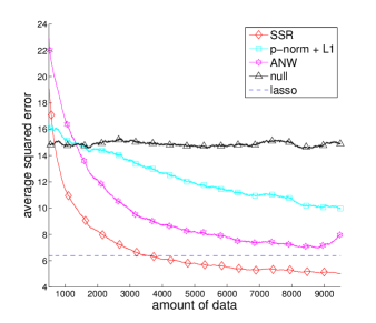
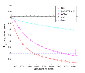
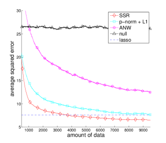
Prediction Error Parameter Error Linear Regression, i.i.d. Features Linear Reg., Correlated Features Logistic Regression

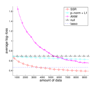
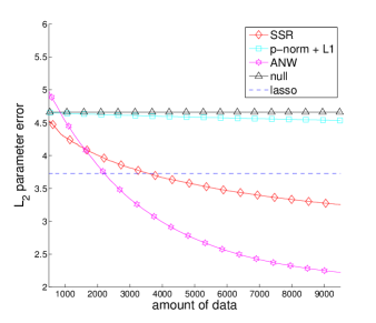
Figure 2: Simulation results. The prediction error is in terms of Huberized quadratic loss or logistic loss. We ran each algorithm with $T=10,000$ training examples in total. The spike in error for ANW in the first row is because ANW is an epoch-based algorithm, and error tends to increase temporarily at the start of a new epoch.

Figure 2 compares the performance of each algorithm, in terms of both prediction error and parameter error. The prediction error at time $t$ is $f_{t}(w_{t})$, where $w_{t}$ depends only on $(x_{1:t-1},y_{1:t-1})$, so that prediction error measures actual generalization ability and hence penalizes overfitting. Results are aggregated over 10 realizations of the dataset for a fixed $w^{*}$. The prediction error is averaged over a sliding window consisting of the latest 1,000 examples. In addition, timing information for all algorithms is given in Table 1.

We first compare the online algorithms. Both SSR and ANW converge in squared error at a $\frac{1}{T}$ rate, while the $p$-norm algorithm converges at only a $\frac{1}{\sqrt{T}}$ rate. This can be seen in most of the plots, where SSR and ANW both outperform the $p$-norm algorithm; the exception is in the correlated inputs case, where the $p$-norm algorithm outperforms ANW in prediction error by a large margin and is not too much worse than SSR. The reason is that the $p$-norm algorithm is highly robust to correlations in the data, while ANW and SSR rely on restricted strong convexity and irrepresentability conditions, respectively, which tend to degrade as the inputs become more correlated.

We also note that, in comparison to other methods, ANW performs better in terms of parameter error than prediction error. The difference is particularly striking for the logistic regression task, where ANW has very poor prediction error but very good parameter error (substantially better than all other methods). The fact that ANW incurs large losses while achieving low parameter error in the classification example is not contradictory because, with logistic regression, it is possible to obtain high prediction accuracy without recovering the optimal parameters.

Comparison with the lasso fit by glmnet, which we treat as an oracle, yields some interesting results. Recall that the lasso was only trained using 2,500 training examples, as this was the most data glmnet could handle before crashing. When the streaming methods have access to only 2,500 examples as well, the lasso is beating all of them, just as we would expect. However, as we bring in more data, our SSR method starts to overtake it: in all examples, our method achieves lower prediction error around 4,000 training examples. This phenomenon emphasizes the fact that, with large datasets, having computationally efficient algorithms that let us work with more data is desirable.

Finally we note that, in terms of runtime, SSR is by far the fastest method, running 4 to 10 times faster than either of the two other algorithms. We emphasize that none of these methods were optimized, so the runtime of each method should be taken as a rough indicator rather than an exact measurement of efficiency. The bulk of the runtime difference among the online algorithms is due to the fact that both ANW and the $p$-norm algorithm require expensive floating point operations like taking $p$-th powers, while SSR requires only basic floating point operations like multiplication and addition.

Tuning

We selected the tuning parameters using a single development set of size $1,000$. The tuning parameters for $p$-norm and ANW are a step size and $L_{1}$ penalty, and the tuning parameters for SSR are the constants $\epsilon$, $\alpha$, and $\lambda$ in Algorithm 1, the first two of which control the step size and the last of which controls the $L_{1}$ penalty.

3.2 Genomics Data

The dataset, collected by the Wellcome Trust Case Control Consortium [10], is a genome-wide association study, comparing $d=500,568$ single nucleotide polymorphisms (SNPs). The dataset contains 2,000 cases of type 1 diabetes (T1D), and 1,500 controls, for a total of $T=3,500$ data points. We coded each SNP as 0 if it matches the wild type allele, and as 1 else.

We compared the same methods as before, using a random subset of $500$ data points for tuning hyperparameters (since the dataset is already small, we did not create a separate development set). We only compute prediction error since the true parameters are unknown. In Figure 3, we plot the prediction error averaged over $40$ random permutations of the data and over a sliding window of length $500$. The results look largely similar to our simulations. As before, SSR outperforms the other streaming methods, and eventually also beats the lasso oracle once it is able to see enough training data.

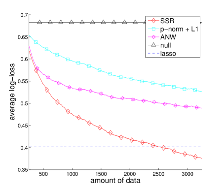
Figure 3: Genomics example; logistic loss vs. amount of data.

4 Adaptive Mirror Descent with Sparsity Guarantees

We now begin to flesh out the intuition described in Section 2.4. Our first goal is to provide an analogue to the mirror descent bound in Proposition 2.4 that takes advantage of sparsity. Intuitively, online algorithms with sparse weights $\left\lVert w_{t}\right\rVert_{0}\leq k$ should behave as though they were evolving in a $k$-dimensional space instead of a $d$-dimensional space. However, the baseline bound (20) does not take advantage of this at all: it depends on $\|\nabla f_{t}(w_{t})\|_{2}^{2}$, which could be as large as $B^{2}d$.

In this section, we strengthen the adaptive mirror descent bound of Orabona et al. [41] in a way that reflects the effective sparsity of the $w_{t}$. We state our results in the standard adversarial setup. Statistical assumptions will become important in order to bound the cost of $L_{1}$-penalization (Section 5).

Our main result that strengthens the adaptive mirror descent bound is Lemma 4.1, which replaces the Bregman divergence term $D_{\psi_{t}^{*}}\left(\theta_{t+1}||\theta_{t}\right)$ in (17) with the smaller term $D_{\psi_{t}^{*}}\left(\theta_{t+1}{\scriptstyle[S_{t}]}||\theta_{t}{\scriptstyle[S_{t}]}\right)$, which measures only the divergence over a subset $S_{t}$ of the coordinates. As before, $\theta_{t+1}{\scriptstyle[S_{t}]}$ denotes the coordinates of $\theta_{t+1}$ that belong to $S_{t}$, with the rest of the coordinates zeroed out. We also let $\operatorname{supp}(w_{t})$ denote the set of non-zero coordinates of $w_{t}$. Throughout, we defer most proofs to the appendix.

Lemma 4.1 (adaptive mirror descent with sparsity).

Suppose that adaptive mirror descent (15) is run with convex regularizers $\psi_{t}$, and let $S_{t}$ be a set satisfying:

1. $\operatorname{supp}(w_{t})\subseteq S_{t}$

2. $\operatorname{supp}(w_{t+1})\subseteq S_{t}$

3. For all $w{\scriptstyle[S_{t}]}$, $\psi_{t}(w{\scriptstyle[S_{t}]},\tilde{w}{\scriptstyle[\neg S_{t}]})$ is minimized at $\tilde{w}{\scriptstyle[\neg S_{t}]}=0$.

Then,

$$\sum_{t=1}^{T} \left(w_{t}-u\right)^{\top}\nabla f_{t}(w_{t})$$ (29)

$$\leq\psi_{T}(u)+\sum_{t=1}^{T}D_{\psi^{*}_{t}}\left(\theta_{t+1}{\scriptstyle[S_{t}]}||\theta_{t}{\scriptstyle[S_{t}]}\right)+\sum_{t=1}^{T}[\psi_{t-1}(w_{t})-\psi_{t}(w_{t})].$$

We emphasize that this result does not require any statistical assumptions about the data-generating process, and relies only on convex optimization machinery. Later, we will use statistical assumptions to control the size of the active set $S_{t}$ and thus bound the right-hand-side of (29).

If we apply Lemma 4.1 to the choice of $\psi_{t}$ given in (54), we get Lemma 4.2 below. The resulting bound is identical to the one in (2.5), except we have replaced $\|\nabla f_{t}(w_{t})\|_{2}^{2}$ with a term that depends only on an effective dimension $k_{t}$.

Lemma 4.2 (decomposition with sparsity).

Let $f_{t}(\cdot)$ be a sequence of convex loss functions, and let $w_{t}$ be selected by adaptive mirror descent with regularizers (54). Then

$$\sum_{t=1}^{T} \left(w_{t}-u\right)^{\top}\nabla f_{t}\left(w_{t}\right)\leq\Omega+\Lambda+Q,\text{ where }$$ (30)

$$\Omega =\frac{\epsilon}{2}\left\lVert u\right\rVert_{2}^{2}+\frac{B^{2}}{2}\sum_{t=1}^{T}\frac{k_{t}}{\epsilon+\eta\,t},$$ (31)

$\Omega$ replaces $\Omega_{0}$ in Corollary 2.5, and $\Lambda$ and $Q$ are defined in (22) and (23). Here, $k_{t}=\left\lvert S_{t}\right\rvert$ is the number of active features, and we take $S_{t}=\cup_{s=1}^{t+1}\operatorname{supp}(w_{s})$.

Example: forcing sparsity

The statement of Lemma 4.2 is fairly abstract, and so it can be helpful to elucidate its implications with some examples. First, suppose that we determine the $\lambda_{t}$ sequence in such a way to force the $w_{t}$ to be $k$-sparse:

$$\lambda_{t+1}=\max\left\{\lambda_{t},\,\left|\theta_{t}\right|^{(k+1,\,d)}+B\right\},$$ (32)

where $|\theta_{t}|^{(k+1,\,d)}$ denotes the $(k+1)$-st largest (in absolute magnitude) coordinate of $\theta_{t}$. Also suppose that we set $\eta=0$ for simplicity. Then, we can simplify our result to the following:

Corollary 4.3 (simplification with sparsity).

Under the conditions of Lemma 4.2, suppose that $\lambda_{t}$ is set using (32), $\eta=0$, and that the $f_{t}(\cdot)$ are convex. Then, we obtain the regret bound

$$\operatorname{Regret}(u)\leq\frac{\epsilon R^{2}}{2}+\frac{1}{2\epsilon}kB^{2}T+\lambda_{T}R.$$ (33)

If we optimize the bound with $\epsilon=\frac{B}{R}\sqrt{kT}$, then (33) is equal to $R\left(B\sqrt{kT}+\lambda_{T}\right)$.

Proof.

By convexity of $f_{t}$, we have $f_{t}(w_{t})-f_{t}(u)\leq(w_{t}-u)^{\top}\nabla f_{t}(w_{t})$. Also, since $\eta=0$, we can actually take $S_{t}=\operatorname{supp}(w_{t})\cap\operatorname{supp}(w_{t+1})$ and still satisfy the conditions of Lemma 4.1. To get the RHS of (33) from (30), we use the inequalities $k_{t}=|S_{t}|\leq k$, $\left\lVert u\right\rVert_{2}\leq\left\lVert u\right\rVert_{1}\leq R$ and $(\lambda_{t-1}-\lambda_{t})\|w_{t}\|_{1}\leq 0$; this latter inequality implies that $\sum_{t=1}^{T}(\lambda_{t-1}-\lambda_{t})(\|w_{t}\|_{1}-\|u\|_{1})\leq\lambda_{T}\|u\|_{1}$. ∎

We have shown that stochastic gradient descent can achieve regret that depends on the sparsity level $k$ rather than the ambient dimension $d$, as long as the $L_{1}$ penalty is large enough. Previous analyses [e.g., 60] had an analogous regret bound of $R(B\sqrt{dT}+\lambda_{T})$, which could be substantially worse when $d$ is large.

4.1 Interlude: Sparse Learning with Strongly Convex Loss Functions

In the above section we showed that, when working with generic convex loss functions $f_{t}$, we could use our framework to improve a $\sqrt{dT}$ factor into $\sqrt{kT}$; in other words, we could bound the regret in terms of the effective dimension $k$ rather than the ambient dimension $d$. We can thus achieve low regret in high dimensions while using an $L_{2}$-regularizer, as opposed to previous work [51] that used an $L_{p}$-regularizer with $p=\frac{2\log(d)}{2\log(d)-1}$. This fact becomes significant when we consider strong convexity properties of our loss functions, where it is advantageous to use a regularizer with the same strong convexity structure as the loss, and where $L_{2}$-strong convexity of the loss function is much more common than strong convexity in other $L_{p}$-norms.

In the standard online convex optimization setup, it is well known [17, 28] that if the loss functions $f_{t}$ are strongly convex, we can use faster learning rates to get excess risk on the order of $\log T$ rather than $\sqrt{T}$. This is because the strong convexity of $f_{t}$ allows us to remove the $\sum_{t=1}^{T}\|w_{t}-u\|_{2}^{2}$ term from bounds like (30).

In practice, the loss function $f_{t}$ is only strongly convex in expectation, and we will analyze this setting in Section 6. But as a warm-up, let us analyze the case where each $f_{t}$ is actually strongly convex. In this case, we can remove the $Q$ term from our regret bound (30) entirely:

Theorem 4.4 (decomposition with sparsity and strong convexity).

Suppose that we are given a sequence of $\alpha$-strongly convex losses $f_{1},\,\ldots,\,f_{T}$, and that we run adaptive mirror descent with the regularizers $\psi_{t}$ from (54) with $\eta=\alpha$. Then, using $\Omega$ and $\Lambda$ from (30), we have

$$\operatorname{Regret}(u)=\sum_{t=1}^{T} \left(f_{t}\left(w_{t}\right)-f_{t}\left(u\right)\right)\leq\Omega+\Lambda.$$ (34)

The key is that with $f_{t}$ $\alpha$-strongly convex, we have $f_{t}\left(w_{t}\right)-f_{t}\left(u\right)\leq\nabla f_{t}(w_{t})^{\top}\left(w_{t}-u\right)-\frac{\alpha}{2}\|w_{t}-u\|_{2}^{2}$, from which the result follows by invoking (30). As a result, we can remove the $Q$ term while still allowing $\eta>0$, which can help reduce $\Omega$.

Example: forcing sparsity

We can again use the sparsity-forcing schedule $\lambda_{t}$ from (32) to gain some intuition.

Corollary 4.5 (simplification with sparsity and strong convexity).

Under the conditions of Theorem 4.4, suppose that we set $\lambda_{t}$ using (32) and set $\epsilon=0$. Then

$$\operatorname{Regret}(u)\leq\frac{kB^{2}}{2\alpha}\left(1+\log T\right)+\lambda_{T}\left\lVert u\right\rVert_{1}.$$ (35)

At first glance, it may seem that this result gives us an even better bound than the one stated in Theorem 2.1. The main term in the bound (35) scales as $\log T$ and has no explicit dependence on $d$. However, we should not forget the $\lambda_{T}\left\lVert u\right\rVert_{1}$ term required to keep the weights sparse: in general, even if all but a small number of coordinates of $\nabla f_{t}(w_{t})$ are zero-mean random noise, $\lambda_{T}$ will need to grow as $\sqrt{T}$ (in fact, $\sqrt{T\log(d)}$) in order to preserve sparsity. This is because an unbiased random walk will still have deviation $\sqrt{T}$ from zero after $T$ steps. Thus, although we managed to make the main term of the regret bound small, the $\lambda_{T}\left\lVert u\right\rVert_{1}$ term still looms. In the absence of strong convexity, having $\lambda_{T}=O(\sqrt{T})$ would be acceptable since the first two terms of (33) would grow as $\sqrt{T}$ anyway in this case, but since we are after a $\log T$ dependence, we need to work harder.

In the next section, we will show that, if we make statistical assumptions and restrict our attention to the minimizer $w^{*}$ of $\mathcal{L}$, the cost of penalization becomes manageable. Specifically, we will show that the $\sum_{t=1}^{T}\left(\lambda_{t-1}-\lambda_{t}\right)\left\lVert w_{t}\right\rVert_{1}$ term in (34) mostly cancels out the problematic $\lambda_{T}\left\lVert u\right\rVert_{1}$ term when $u=w^{*}$, and that the remainder scales only logarithmically in $T$.

5 The Cost of Sparsity

In the previous section, we showed how to control the main term of an adaptive mirror descent regret bound by exploiting sparsity. In order to achieve sparsity, however, we had to impose an $L_{1}$ penalty which introduces a cost of sparsity term (22), which is:

$$\Lambda \stackrel{{\scriptstyle\mathrm{def}}}{{=}}\sum_{t=1}^{T}\left(\lambda_{t-1}-\lambda_{t}\right)\left(\left\lVert w_{t}\right\rVert_{1}-\left\lVert w^{*}\right\rVert_{1}\right).$$ (36)

Before, our regret bounds (34) held against any comparator $u\in\mathcal{H}$, but all the results in this section rely on statistical assumptions and thus will only hold when $u=w^{*}$, the expected risk minimizer.

In general, we will need $\lambda_{T}$ to scale as $\sqrt{T\log d}$ to ensure sparsity. If we use the naive upper bound $\Lambda=\lambda_{T}\left\lVert w^{*}\right\rVert_{1}+\sum_{t=1}^{T}\left(\lambda_{t-1}-\lambda_{t}\right)\left\lVert w_{t}\right\rVert_{1}\leq\lambda_{T}\left\lVert w^{*}\right\rVert_{1}$, which holds so long as $\lambda_{t}\geq\lambda_{t-1}$, we again get regret bounds that grow as $\sqrt{T}$, even under statistical assumptions. However, we can do better than this naive bound: we will show that it is possible to substantially cut the cost of sparsity by using an $L_{1}$ penalty that grows steadily in $t$; in our analysis, we use $\lambda_{t}=\lambda\sqrt{t+1}$. Using Assumptions (1-3) from Section 2, we can obtain bounds for $\Lambda$ that grow only logarithmically in $T$:

Lemma 5.1 (cost of sparsity).

Suppose that Assumptions (1-3) of Section 2 hold, and that $\lambda_{t}=\lambda\sqrt{t+1}$. Then, for any $\delta>0$, with probability $1-\delta$,

$$\Lambda\leq\frac{\lambda}{2}\,\sqrt{k\left(1+\log T\right)}$$ (37)

$$\ \ \ \ \ \ \times\sqrt{\frac{4}{\alpha}\sum_{t=1}^{T}\left(f_{t}\left(w_{t}{\scriptstyle[S]}\right)-f_{t}\left(w^{*}\right)\right)+\frac{9kB^{2}\log\left(\log_{2}(2T)/\delta\right)}{4\alpha^{2}}}.$$

Note that Lemma 5.1 bounds $\Lambda$ in terms of what is essentially the square root of $\operatorname{Regret}(w^{*})$. Indeed, if $\operatorname{supp}(w_{s})\subseteq S$, so that $w_{t}{\scriptstyle[S]}=w_{t}$, then the sum appearing inside the square-root is exactly $\operatorname{Regret}(w^{*})$. Using this bound, we can provide a recipe for transforming regret bounds for $L_{1}$-penalized adaptive mirror descent algorithms into much stronger excess risk bounds.

Theorem 5.2 (cost of sparsity for online prediction error).

Under the conditions of Lemma 5.1, suppose that we have any excess risk bound of the form

$$\operatorname{Regret}(w^{*})\leq R_{T}\left(w^{*}\right)+\Lambda$$ (38)

for some main term $R_{T}(w^{*})\geq 0$ and $\Lambda$ as defined in (36). Then, for regularization schedules of the form $\lambda_{t}=\lambda\sqrt{t+1}$, the following excess risk bound also holds with probability $1-\delta$ for any $\delta>0$:

$$\operatorname{Regret}(w^{*})\leq 2R_{T}\left(w^{*}\right)$$ (39)

$$\ \ \ \ +\frac{4k\lambda^{2}\left(1+\log T\right)}{3\alpha}+\frac{kB^{2}\log\left(\log_{2}(2T)/\delta\right)}{2\alpha}+\max\left(0,-\Delta\right),$$

$$\ \ \ \ \text{where }\Delta=\sum_{t=1}^{T}\left(f_{t}\left(w_{t}\right)-f_{t}\left(w_{t}{\scriptstyle[S]}\right)\right).$$

Notice that this result does not depend on any form of orthogonal noise or irrepresentability assumption. Instead, our bound depends implicitly on the assumption that sparsification improves the performance of our predictor. Specifically, $\Delta$ is the excess risk we get from using non-zero weights outside the sparsity set $S$. If the non-signal features are pure noise (i.e., independent from the response), then clearly

$$\mathbb{E}\left[f_{t}(w_{t}{\scriptstyle[S]})\right]\leq\mathbb{E}\left[f_{t}(w_{t})\right],$$

and so $\mathbb{E}\left[\Delta\right]\geq 0$ and thus (39) is a strong bound in the sense that the cost of sparsity grows only as $\log T$. Conversely, if there are many good non-sparse models, then $-\Delta$ could potentially be large enough to render the bound useless.

To use Theorem 5.2 in practice, we will make assumptions (such as irrepresentability) that guarantee that $\operatorname{supp}(w_{t})\subseteq S$ with high probability for all $t$, so that $w_{t}{\scriptstyle[S]}=w_{t}$ and thus $\Delta=0$. The following result gives us exactly this guarantee in the case where the noise features $\neg S$ are orthogonal to the signal $S$ (formalized as Assumption 4), by letting $\lambda_{t}$ grow at an appropriate rate. In Section 8, we relax the orthogonality assumption to one where the noise features need only be irrepresentable.

Lemma 5.3 (support recovery with uncorrelated noise).

Suppose that Assumptions 1, 3, and 4 hold. Then, for any convex functions $\{\zeta_{t}^{i}\}_{i=1}^{d}$, as long as $\zeta_{t}^{i}$ is minimized at $0$ for all $i\not\in S$, the weights $w_{t}$ generated by adaptive mirror descent with regularizer

$$\psi_{t}\left(w\right)=\sum_{i=1}^{d}\zeta_{t}^{i}\left(w^{i}\right)+\lambda_{t}\left\lVert w\right\rVert_{1}$$

and

$$\lambda_{t}=c_{\delta}\sqrt{t}\;\text{ with }\;c_{\delta}=\frac{3B}{2}\sqrt{\log\left(\frac{2d\log_{2}(2T)}{\delta}\right)}$$ (40)

will satisfy $\operatorname{supp}(w_{t})\subseteq S$ for all $t=1,\,\dots,\,T$ with probability at least $1-\delta$.

We have thus cleared the main theoretical hurdle identified at the end of Section 4.1, by showing that having an $L_{1}$ penalty that grows as $\sqrt{t}$ does not necessarily make the regret bound scale with $\sqrt{t}$ also. Thus, we can now use Theorem 5.2 in combination with Lemma 5.3 to get logarithmic bounds on the cost of sparsity $\Lambda$ for strongly convex losses, as shown below.

Corollary 5.4 (synthesis).

Suppose that Assumptions 1, 3, and 4 hold, that we run Algorithm 1 with $\varepsilon=0$ and $\lambda_{t}=c_{\delta}\sqrt{t}$ with $c_{\delta}$ as defined in (40). Moreover, suppose that the loss functions $f_{t}$ are all $\alpha$-strongly convex for some $\alpha>0$ and that we set $\eta=\alpha$. Then,

$$\sum_{t=1}^{T}\left(f_{t}(w_{t})-f_{t}(w^{*})\right)=\mathcal{O}_{P}\left(\frac{kB^{2}}{\alpha}\log\left(d\log\left(T\right)\right)\log\left(T\right)\right).$$

Proof.

This result follows directly by combining Theorem 4.4 with Theorem 5.2, while using Lemma 5.3 to control sparsity. ∎

6 Online Learning with Strong Convexity in Expectation

Thus far, we have obtained our desired regret bound of $\mathcal{O}_{P}\left(k\log(d\log(T))\log(T)\right)$, but assuming that each loss function $f_{t}$ was $\alpha$-strong convexity (Corollary 5.4). This strong convexity assumption, however, is unrealistic for many commonly-used loss functions. For example, in the case of linear regression with $f_{t}(w)=\frac{1}{2}(y_{t}-w^{\top}x_{t})^{2}$, the individual loss functions $f_{t}$ are not strongly convex. However, we do know that the $f_{t}$ are strongly convex in expectation as long as the covariance of $x$ is non-singular. In this section, we show that this weaker assumption of strong convexity in expectation is all that is needed to obtain the same rates as before.

The adaptive mirror descent bounds presented in Sections 2 and 4 all depend on the following inequalities: if the loss function $f_{t}(\cdot)$ is convex, then

$$f_{t}\left(w_{t}\right)-f_{t}\left(u\right)\leq\left(w_{t}-u\right)^{\top}\nabla f_{t}\left(w_{t}\right),$$ (41)

and if $f_{t}(\cdot)$ is $\alpha$-strongly convex, then

$$f_{t}\left(w_{t}\right)-f_{t}\left(u\right)\leq\left(w_{t}-u\right)^{\top}\nabla f_{t}\left(w_{t}\right)-\frac{\alpha}{2}\|w_{t}-u\|_{2}^{2}.$$ (42)

It turns out that we can use similar arguments even when the losses $f_{t}(\cdot)$ are not convex, provided that $f_{t}(\cdot)$ is convex in expectation. The following lemma is the key technical device allowing us to do so. Comparing (43) with (42), notice that we only lose a factor of $2$ in terms of $\alpha$ and pick up an additive constant for the high probability guarantee.

Lemma 6.1 (online prediction error with expected strong convexity).

Let $f_{1},\,\ldots,\,f_{T}$ be a sequence of (not necessarily convex) loss functions defined over a convex region $\mathcal{H}$ and let $u,\,w_{1},\,\ldots,\,w_{T}\in\mathcal{H}$. Finally let $\mathcal{F}_{0},\mathcal{F}_{1},\ldots$ be a filtration such that:

1. $w_{t}$ is $\mathcal{F}_{t-1}$-measurable, and $u$ is $\mathcal{F}_{0}$-measurable,

2. $f_{t}$ is $\mathcal{F}_{t}$-measurable and $\mathbb{E}\left[f_{t}\mid\mathcal{F}_{t-1}\right]$ is $\alpha$-strongly convex with respect to some norm $\left\lVert\cdot\right\rVert$, and

3. $f_{t}$ is almost surely $L$-Lipschitz with respect to $\left\lVert\cdot\right\rVert$ over all of $\mathcal{H}$.

Then, with probability at least $1-\delta$, we have, for all $T\geq 0$,

$$\operatorname{Regret}(u) \leq\sum_{t=1}^{T}\left(\left(w_{t}-u\right)^{\top}\nabla f_{t}\left(w_{t}\right)-\frac{\alpha}{4}\|w_{t}-u\|^{2}\right)+\frac{8L^{2}\log(1/\delta)}{\alpha}.$$ (43)

We can directly use this lemma to get an extension of the adaptive mirror descent bound of Orabona et al. [41] for loss functions that are only convex in expectation, thus yielding an analogue of Theorem 4.4, that only requires expected strong convexity instead of strong convexity. Note that the above result holds for any fixed $u$, although we will always invoke it for $u=w^{*}$.

Theorem 6.2 (simplification with expected strong convexity).

Suppose that the $f_{t}(\cdot)$ are a sequence of loss functions satisfying Assumptions (1-4), and that we run adaptive mirror descent with the regularizers $\psi_{t}$ from (54) and $\varepsilon=0$. Then, assuming that  $\operatorname{supp}(w_{t})\subseteq S$ for all $t$, we have that for any $\delta>0$, with probability at least $1-\delta$,

$$\operatorname{Regret}(w^{*})\leq\frac{kB^{2}}{\alpha}\left({1+\log T}+8\log\left(\frac{1}{\delta}\right)\right)+\Lambda,$$ (44)

where $\Lambda$ is the cost of sparsity as defined in (22).

We have now assembled all the necessary ingredients to establish our first main result, namely the excess empirical risk bound for Algorithm 1 given in Theorem 2.1, which states that

$$\operatorname{Regret}(w^{*})=\mathcal{O}_{P}\left(\frac{kB^{2}}{\alpha}\log\left({d\log(T)}\right)\log(T)\right).$$

The proof, provided at the end of Section A.4, follows directly from combining Theorem 5.2, Lemma 5.3, and Theorem 6.2.

We pause here to discuss what we have done so far. At the beginning of Section 4, we set out to provide an excess loss bound for the sparsified stochastic gradient method described in Algorithm 1. The main difficulty was that although $L_{1}$-induced sparsity enabled us to control the size of the main term $\Omega$ from (31), it induced another cost-of-sparsity term $\Lambda$ (22) that seemingly grew as $\sqrt{T}$. However, through the more careful implicit analysis presented in Section 5, we were able to show that, if $\Omega$ satisfies logarithmic bounds in $d$ and $T$, then $\Lambda$ must also satisfy similar bounds. In parallel, we showed in Section 6 how to work with expected strong convexity instead of actual strong convexity.

The ideas discussed so far, especially in Section 5, comprise the main technical contributions of this paper. In the remaining pages, we extend the scope of our analysis, by providing an analogue to Theorem 2.1 that lets us control parameter error at a quasi-optimal rate, and by extending our analysis to designs with correlated noise features.

7 Parameter Estimation using Online-to-Batch Conversion

In the previous sections, we focused on bounding the cumulative excess loss made by our algorithm while streaming over the data, namely $\sum_{t=1}^{T}(f_{t}(w_{t})-f_{t}(w^{*}))$. In many cases, however, a statistician may be more interested in estimating the underlying weight vector $w^{*}$ than in just obtaining good predictions. In this section, we show how to adapt the machinery from the previous section for parameter estimation.

The key idea is as follows. Assume that the $f_{t}$ are i.i.d. and recall the expected risk is defined as $\mathcal{L}\left(w\right)=\mathbb{E}\left[f_{t}\left(w\right)\right]$. If we know that $\mathcal{L}\left(\cdot\right)$ is $\alpha$-strongly convex, we immediately see that, for any $w$,

$$\frac{1}{2}\left\lVert w-w^{*}\right\rVert_{2}^{2}\leq\frac{1}{\alpha}\left(\mathcal{L}\left(w\right)-\mathcal{L}\left(w^{*}\right)\right).$$ (45)

Thus, given a guess $\hat{w}_{t}$, we can transform any generalization error bound on $\mathcal{L}\left(\hat{w}_{t}\right)-\mathcal{L}\left(w^{*}\right)$ into a parameter error bound for $\hat{w}_{t}$.

The standard way to turn cumulative online loss bounds into generalization bounds is using “online-to-batch” conversion [13, 31]. In general, online-to-batch type results tell us that if we start with a bound of the form

$$\operatorname{Regret}(w^{*})=\sum_{t=1}^{T}\left(f_{t}(w_{t})-f_{t}(w^{*})\right)=\mathcal{O}_{P}\left(Q(T)\right)$$

for some function $Q(T)$, then

$$\mathcal{L}\left(\hat{w}_{T}\right)-\mathcal{L}\left(w^{*}\right)=\mathcal{O}_{P}\left(\frac{Q(T)}{T}\right),\;\text{with}\;\hat{w}_{T}=\frac{1}{T}\sum_{t=1}^{T}w_{t}.$$

The problem with this approach is that, if we applied online-to-batch conversion directly to Algorithm 1 and Theorem 2.1, we would get a bound of the form

$$\mathcal{L}\left(\hat{w}_{T}\right)-\mathcal{L}\left(w^{*}\right)=\mathcal{O}_{P}\left(\frac{k\log(d\log(T))}{T}\,\log(T)\right),$$

which is loose by a factor $\log T$ with respect to the minimax rate [46]. At a high level, the reason we incur this extra $\log T$ factor is that the required averaging step $\hat{w}_{T}=\frac{1}{T}\sum_{t=1}^{T}w_{t}$ gives too much weight to the small-$t$ weights $w_{t}$, which may be quite far from $w^{*}$.

In this section, however, we will show that if we modify Algorithm 1 slightly, yielding Algorithm 2, we can discard the extra $\log T$ factor and obtain our desired generalization error rate bound of $\mathcal{O}_{P}\left({k\log(d\log(T))}/{T}\right)$. Besides being of direct interest for parameter estimation, this technical result will prove to be important in dealing with correlated noise features under irrepresentability conditions.

To achieve the desired batch bounds, we modify our algorithm as follows:

• We replace the loss functions $f_{t}(w)$ with $\tilde{f}_{t}(w)=tf_{t}(w)$.

• We replace the regularizer $\psi_{t}(w)$ with

  $$\widetilde{\psi}_{t}\left(w\right)=\frac{1}{2\eta}\left(\sum_{s=1}^{t}s\left\lVert w-w_{s}\right\rVert_{2}^{2}\right)+\lambda_{t}\left\lVert w\right\rVert_{1}.$$ (46)

• We use a correspondingly larger $L_{1}$ regularizer $\lambda_{t}=\lambda\cdot t^{3/2}$.

Procedurally, this new method yields Algorithm 2. Intuitively, the new algorithm pays more attention to later loss functions and weight vectors compared to earlier ones.

This construction will allow us to give bounds for

$$\frac{1}{T}\sum_{t=1}^{T}t\left(f_{t}\left(w_{t}\right)-f_{t}\left(w^{*}\right)\right)\;\text{instead of}\;\sum_{t=1}^{T}\left(f_{t}\left(w_{t}\right)-f_{t}\left(w^{*}\right)\right).$$ (47)

It turns out that while the latter is only bounded by $\mathcal{O}_{P}\left(\log(T)\right)$, the former is bounded by $\mathcal{O}_{P}\left(1\right)$. This is useful for proving generalization bounds, as shown by the following online-to-batch conversion result, the proof of which relies on martingale tail bounds similar to those developed by Freedman [22] and Kakade and Tewari [31]. Note that the weight averaging scheme used in Algorithm 2 gives us exactly

$$\hat{w}_{t}=\frac{2}{t(t+1)}\sum_{s=1}^{t}s\,w_{s};$$

this equality can be verified by induction.

Proposition 7.1 (online-to-batch conversion).

Suppose that, for any $\delta>0$, with probability $1-\delta$,

$$\sum_{s=1}^{t}s\left(f_{s}\left(w_{s}\right)-f_{s}\left(w^{*}\right)\right)\leq R_{\delta}\,t$$

for all $t\leq T$, and that each $f_{t}$ is $L$-Lipschitz and $\alpha$-strongly convex over $\mathcal{H}$. Then, with probability at least $1-2\delta$,

$$\mathcal{L}\left(\hat{w}_{t}\right)-\mathcal{L}\left(w^{*}\right) \leq\frac{4R_{\delta}}{t}+\frac{9\log\left(\log_{2}(2T^{3})/\delta\right)L^{2}}{\alpha t}$$ (48)

for all $t\leq T$.

Given these ideas, we can mimic our analysis from Sections 4, 5 and 6 to provide bounds of the form (47) for Algorithm 2. Combined with Proposition 7.1, this will result in the desired generalization bound. For conciseness, we defer this argument to the Appendix, and only present the final bound below.

Theorem 7.2 (expected prediction error with uncorrelated noise).

Suppose that we run Algorithm 2 with $\eta=\alpha/2$ and

$$\lambda=\frac{3B}{2}\sqrt{\log\left(\frac{2d\log_{2}(2T^{3})}{\delta}\right)},$$

and that Assumptions 1-4 hold. Then, with probability $1-3\delta$, for all $t\leq T$ we have

$$\mathcal{L}\left(\hat{w}_{t}\right)-\mathcal{L}(w^{*})\leq\frac{269B^{2}k\log\left(2d\log_{2}(2T^{3})/\delta\right)}{\alpha t},$$ (49)

and hence

$$\frac{1}{2}\left\lVert\hat{w}_{t}-w^{*}\right\rVert_{2}^{2}\leq\frac{269B^{2}k\log\left(2d\log_{2}(2T^{3})/\delta\right)}{\alpha^{2}t}.$$ (50)

With this result in hand, we can obtain Theorem 2.2 as a direct corollary of Theorem 7.2. Thus, as desired, we have obtained a parameter error bound that decays as $\mathcal{O}_{P}\left(k\log\left(d\log(T)\right)/T\right)$. As discussed earlier, this is minimax optimal [46] as long as the problem is not extremely low-dimensional (the bound becomes loose only if $T\gg\exp(d)$).

8 Streaming Sparse Regression with Irrepresentable Features

Finally, we end our analysis by re-visiting probably the most problematic of our original 4 assumptions from Section 2.1, namely that the gradients corresponding to noise features are all mean zero for any weight vector $w$ with support in $S$. Here, we show that this assumption is in fact not needed in its full strength. In particular, in the case of streaming linear regression, a weaker irrepresentability condition (Assumption 5) is sufficient to guarantee good performance of our algorithm.

In our original analysis, mean-zero gradients (Assumption 4) allowed us to guarantee that our $L_{1}$ penalization scheme would in fact result in sparse weights, as in Lemma 5.3. Below, we provide an analogous result in the case of irrepresentable noise features.

Lemma 8.1 (support recovery with irrepresentability).

Suppose that Assumptions 1-3 and 5 hold, and that we run Algorithm 2 with $\eta=\alpha/2$ and

$$\lambda\geq\sqrt{\frac{228B^{2}\log\left({2d\log_{2}(2T^{3})}\big{/}{\delta}\right)}{1-24\rho^{2}}}.$$ (51)

Then, with probability at least $1-4\delta$, $\operatorname{supp}(w_{t})\subseteq S$ for all $t=1,\,\dots,\,T$.

Thanks to this sparsity guarantee, we can use similar machinery as in Section 7 to bound the generalization error of the output of Algorithm 2. Again, just like in Section 7, Theorem 2.3 is a direct consequence of the result below thanks to the $\alpha$-strong convexity of $\mathcal{L}$ and (45).

Theorem 8.2 (expected prediction error with irrepresentability).

Let $w_{t}$ be the weights generated by Algorithm 2. Then, under the conditions of Lemma 8.1, with $\hat{w}_{T}=\frac{2}{T(T+1)}\sum_{t=1}^{T}t\,w_{t}$, we have, with probability $1-5\delta$, $\operatorname{supp}(\hat{w_{T}})\subseteq S$ and

$$\mathcal{L}\left(\hat{w}_{T}\right)-\mathcal{L}\left(w^{*}\right) =\mathcal{O}_{P}\left(\frac{1}{1-24\rho^{2}}\,\frac{kB^{2}\log\left(d\log(T)\right)}{\alpha T}\right),$$ (52)

$$\left\lVert\hat{w}_{T}-w^{*}\right\rVert_{2}^{2} =\mathcal{O}_{P}\left(\frac{1}{1-24\rho^{2}}\,\frac{kB^{2}\log\left(d\log(T)\right)}{\alpha^{2}T}\right).$$ (53)

9 Discussion

In this work, we have developed an efficient algorithm for solving sparse regression problems in the streaming setting, and have shown that it can achieve optimal rates of convergence in both prediction and parameter error. To recap our theoretical contributions: we have shown that online algorithms with sparse iterates enjoy better convergence (obtaining a dependence on $k$ rather than $d$); that regularization schedules increasing at a $\sqrt{t}$ rate can enjoy very low excess risk under statistical assumptions; and that functions that are only strongly convex in expectation can still yield $\log T$ error rather than $\sqrt{T}$. Together, these show that a natural streaming analogue of the lasso achieves convergence at the same rate as the lasso itself, similarly to how stochastic gradient descent achieves the same rate as batch linear regression.

This work generates several questions. First, can we weaken the irrepresentability assumption, or more ambitiously, replace it with a restricted isometry condition? This latter goal would require analyzing the algorithm in regimes where the support is not recovered, since the restricted isometry property is not enough to guarantee support recovery even in a minimax batch setting. Another interesting question is whether we can reduce memory usage even further — currently, we use $O(d)$ memory, but one could imagine using only $O(k\log(d))$ memory; after all $w^{*}$ takes only $O(k\log(d))$ memory to store.

Finally, we see this work as one part of the broader goal of designing computationally-oriented statistical procedures, which undoubtedly will become increasingly important in an era when high volumes of streaming data is the norm. By leveraging online convex optimization techniques, we can analyze specific procedures, whose computational properties are favorable by construction. By using statistical thinking, we can obtain much stronger results compared to purely optimization-based analyses. We believe that the combination of the two holds general promise, which can be used to examine other statistical problems in a new computational light.

Appendix A Proofs

A.1 Proofs for Section 2

Proof of Corollary 2.5.

We can check that the weights obtained by using the regularizer from (16) can equivalently be obtained using

$$\psi_{t}(w)=\frac{\epsilon}{2}\|w\|_{2}^{2}+\frac{\eta}{2}\sum_{s=1}^{t}\|w-w_{s}\|_{2}^{2}+\lambda_{t}\|w\|_{1}.$$ (54)

We also note that $D_{\psi_{t}^{*}}(\theta_{t+1}||\theta_{t})\leq\frac{1}{2(\epsilon+\eta t)}\|\theta_{t+1}-\theta_{t}\|_{2}^{2}$, which holds because $\psi_{t}$ is $(\epsilon+\eta t)$-strongly convex (see Lemma 2.19 of Shalev-Shwartz [49]). The inequality (20) then follows directly by applying Proposition 2.4 to (54). ∎

A.2 Proofs for Section 4

Proof of Lemma 4.1.

We begin by noting that, given our regularizers $\psi_{t}$, $w_{t,\,i}=0$ if and only if $\left\lvert\theta_{t,\,i}\right\rvert\leq\lambda_{t}$. Now, define

$$\psi^{+}_{t}(w)=\left\{\begin{array}[]{ccl}\psi_{t}(w)&:&w_{i}=0\textrm{ for all }i\not\in S_{t}\\ \infty&:&\textrm{else.}\end{array}\right.$$ (57)

By construction, running adaptive mirror descent with the regularization sequence $\psi^{+}_{t}$ yields an identical set of iterates $\theta_{t}$ as running with the sequence $\psi_{t}$. Moreover, because we also know that all non-zero coordinates of $w_{t}$ are contained in $S_{t-1}$, we can verify that

$$\psi^{+}_{t-1}\left(w_{t}\right)-\psi^{+}_{t}\left(w_{t}\right)=\psi_{t-1}\left(w_{t}\right)-\psi_{t}\left(w_{t}\right),$$

and so using the $\psi^{+}_{t}$ leaves the regret bound (17) from Proposition 2.4 unchanged except for the Bregman divergence terms $\sum_{t=1}^{T}D_{(\psi^{+}_{t})^{*}}(\theta_{t+1}||\theta_{t})$. We can thus bound the regret in terms of $D_{(\psi^{+}_{t})^{*}}(\theta_{t+1}||\theta_{t})$ rather than $D_{\psi_{t}^{*}}(\theta_{t+1}||\theta_{t})$. On the other hand, we see that

$$(\psi^{+}_{t})^{*}(\theta) =\sup_{w}\left\{\left\langle w,\,\theta\right\rangle-\psi^{+}_{t}(w)\right\}$$

$$=\sup_{w{\scriptstyle[S_{t}]}}\left\{\left\langle w{\scriptstyle[S_{t}]},\,\theta{\scriptstyle[S_{t}]}\right\rangle-\psi_{t}(w{\scriptstyle[S_{t}]})\right\}$$

$$=\psi_{t}^{*}(\theta{\scriptstyle[S_{t}]}),$$

where $w{\scriptstyle[S]}$ and $\theta{\scriptstyle[S]}$ denote vectors that are zero on all coordinates not in $S$.

The upshot is that

$$D_{(\psi^{+}_{t})^{*}} (\theta_{t+1}||\theta_{t})$$

$$=\psi_{t}^{*}(\theta_{t+1}{\scriptstyle[S_{t}]})-\left\langle\partial\psi_{t}^{*}(\theta_{t}{\scriptstyle[S_{t}]}),\theta_{t+1}{\scriptstyle[S_{t}]}-\theta_{t}{\scriptstyle[S_{t}]}\right\rangle-\psi_{t}^{*}(\theta_{t}{\scriptstyle[S_{t}]})$$

$$=D_{\psi_{t}^{*}}(\theta_{t+1}{\scriptstyle[S_{t}]}||\theta_{t}{\scriptstyle[S_{t}]}),$$

as was to be shown. ∎

Proof of Lemma 4.2.

We directly invoke Lemma 4.1. First, we check that its conditions are satisfied for $S_{t}=\cup_{s=1}^{t+1}\operatorname{supp}(w_{s})$. Clearly the first two conditions are satisfied by construction, and for the third condition, we note that each term in $\psi_{t}(w)$ is either of the form $\|w\|_{1}$, which pushes all coordinates closer to zero, or $\|w_{s}-w\|_{2}^{2}$ with $s\leq t$, which pushes all coordinates outside of $\operatorname{supp}(w_{s})$ closer to zero. Therefore, the third condition is also satisfied.

Now, we apply the result of Lemma 4.1. The $\psi_{T}(u)$ term in (29) yields

$$\frac{\epsilon}{2}\|u\|_{2}^{2}+\frac{\eta}{2}\sum_{t=1}^{T}\|w_{t}-u\|_{2}^{2}+\lambda_{T}\|u\|_{1},$$ (58)

while the $\sum_{t=1}^{T}[\psi_{t-1}(w_{t})-\psi_{t}(w_{t})]$ term yields

$$\sum_{t=1}^{T}(\lambda_{t-1}-\lambda_{t})\|w_{t}\|_{1}.$$ (59)

The most interesting term is the summation $\sum_{t=1}^{T}D_{\psi_{t}^{*}}(\theta_{t+1}{\scriptstyle[S_{t}]}\|\theta_{t}{\scriptstyle[S_{t}]})$. By standard results on Bregman divergences, we know that if $\psi_{t}$ is $\gamma$-strongly convex, then $\psi_{t}^{*}$ is $\frac{1}{\gamma}$-strongly smooth in the sense that

$$D_{\psi_{t}^{*}}(x\|y)\leq\frac{1}{2\gamma}\|x-y\|_{2}^{2}.$$ (60)

In our case, $\psi_{t}$ is $(\epsilon+\eta t)$-strongly convex, so

$$D_{\psi_{t}^{*}}(\theta_{t+1}{\scriptstyle[S_{t}]}\|\theta_{t}{\scriptstyle[S_{t}]}) \leq\frac{1}{2\gamma}\|\theta_{t+1}{\scriptstyle[S_{t}]}-\theta_{t}{\scriptstyle[S_{t}]}\|_{2}^{2}$$

$$\leq\frac{|S_{t}|}{2(\epsilon+\eta t)}\|\theta_{t+1}-\theta_{t}\|_{\infty}^{2}$$

$$\leq\frac{k_{t}}{2(\epsilon+\eta t)}B^{2},$$

from which the lemma follows. ∎

Proof of Theorem 4.4.

By invoking Lemma 4.2, we have

$$\sum_{t=1}^{T}\partial f_{t}\left(w_{t}\right)^{\top}\left(w_{t}-u\right)\leq\Omega+\Lambda+\frac{\alpha}{2}\sum_{t=1}^{T}\left\lVert u-w_{t}\right\rVert_{2}^{2}.$$ (61)

But now, because $f_{t}(\cdot)$ is $\alpha$-strongly convex, we also know that

$$f_{t}\left(u\right)\geq f_{t}\left(w_{t}\right)+\partial f_{t}\left(w_{t}\right)^{\top}\left(u-w_{t}\right)+\frac{\alpha}{2}\left\lVert u-w_{t}\right\rVert_{2}^{2},$$

implying that

$$\sum_{t=1}^{T}\left(f_{t}\left(w_{t}\right)-f_{t}\left(u\right)\right)\leq\sum_{t=1}^{T}\left(\partial f_{t}\left(w_{t}\right)^{\top}\left(u-w_{t}\right)-\frac{\alpha}{2}\left\lVert u-w_{t}\right\rVert_{2}^{2}\right).$$

Chaining this inequality with (61) gives us (34). ∎

A.3 Proofs for Section 5

Throughout our argument, we will bound certain quantities in terms of themselves. The following auxiliary lemma will be very useful in turning these implicit bounds into explicit bounds.

Lemma A.1.

Suppose that $a,b,c\geq 0$ and $S\leq a+\sqrt{bS+c^{2}}$. Then $S\leq 2a+b+c$.

Proof.

We have $(S-a)^{2}\leq bS+c^{2}$, so that $S^{2}-(2a+b)S+a^{2}-c^{2}\leq 0$. This implies that

$$S \leq\frac{(2a+b)+\sqrt{(2a+b)^{2}-4(a^{2}-c^{2})}}{2}$$

$$=(2a+b)\frac{1+\sqrt{1-4(a^{2}-c^{2})/(2a+b)^{2}}}{2}$$

$$\leq(2a+b)\frac{1+\sqrt{1+4c^{2}/(2a+b)^{2}}}{2}$$

$$\leq(2a+b)\frac{2+\sqrt{4c^{2}}/(2a+b)}{2}$$

$$=2a+b+c,$$

as claimed. The final inequality uses the fact that $\sqrt{x+y}\leq\sqrt{x}+\sqrt{y}$. ∎

It will also be useful to have the following adaptive variant of Azuma’s inequality. Throughout, we use $\log_{2}(x)$ to denote the base-$2$ logarithm of $x$. In interpreting the lemma below, it will be helpful to think of $Z$ as a sum of $T$ independent zero-mean random variables $X_{1:T}$, so that $\mathbb{E}\left[Z\,\big{|}\,\mathcal{F}_{t}\right]-\mathbb{E}\left[Z\right]=X_{1}+\cdots+X_{t}$, and to think of $M_{t}$ as a bound on $|X_{t}|$ that is allowed to depend on $X_{1:t-1}$.

Lemma A.2.

Let $Z$ be a $\mathcal{F}_{T}$-measurable random variable, and let

$$\{\emptyset\}=\mathcal{F}_{0}\subseteq\mathcal{F}_{1}\subseteq...\subseteq\mathcal{F}_{T}$$

be a filtration such that

$$\mathbb{E}\left[Z\,\big{|}\,\mathcal{F}_{t}\right]-\mathbb{E}\left[Z\,\big{|}\,\mathcal{F}_{t-1}\right]\in[A_{t},B_{t}]\text{ almost surely for }t=1,\,...,\,T,$$

where $(A_{t},B_{t})$ is $\mathcal{F}_{t-1}$-measurable, and let $M_{t}=\tfrac{1}{2}(B_{t}-A_{t})$. Moreover, suppose that $\sup_{t=1}^{T}M_{t}\leq\sigma_{1}\sigma_{2}$ with probability $1$ and $\sigma_{1}\geq 1$. Then, for all $\delta>0$, with probability $1-\delta$, we have

$$\mathbb{E}\left[Z\,\big{|}\,\mathcal{F}_{t}\right]-\mathbb{E}\left[Z\right]\geq-\sqrt{\log\left(\frac{\log_{2}(2\sigma_{1}^{2}T)}{\delta}\right)\max\left(2\sigma_{2}^{2},\frac{9}{4}\sum_{s=1}^{t}M_{s}^{2}\right)},$$

for all $t\leq T$.

Proof.

Let $\Delta_{t}=\mathbb{E}\left[Z\,\big{|}\,\mathcal{F}_{t}\right]-\mathbb{E}\left[Z\,\big{|}\,\mathcal{F}_{t-1}\right]$. Note that we have

$$\mathbb{E}\left[\exp\left(-c\Delta_{t}-\frac{c^{2}M_{t}^{2}}{2}\right)\,\big{|}\,\mathcal{F}_{t-1}\right] =\mathbb{E}\left[\exp\left(-c\Delta_{t}\right)\,\big{|}\,\mathcal{F}_{t-1}\right]\exp\left(-\frac{c^{2}M_{t}^{2}}{2}\right)$$

$$\leq\exp\left(\frac{c^{2}M_{t}^{2}}{2}\right)\exp\left(-\frac{c^{2}M_{t}^{2}}{2}\right)$$

$$=1$$

for all $c>0$. Therefore,

$$Y_{t}^{c}\stackrel{{\scriptstyle\mathrm{def}}}{{=}}\exp\left(-c\sum_{s=1}^{t}\Delta_{s}-\frac{c^{2}}{2}\sum_{s=1}^{t}M_{s}^{2}\right)$$

is a supermartingale, and so $\mathbb{P}\left[\sup_{t=1}^{T}Y_{t}^{c}\geq\exp\left(\frac{\gamma c^{2}}{2}\right)\right]\leq\exp\left(-\frac{\gamma c^{2}}{2}\right)$. Noting that $\sum_{s=1}^{t}\Delta_{s}=\mathbb{E}\left[Z\,\big{|}\,\mathcal{F}_{t}\right]-\mathbb{E}\left[Z\right]$, we then have that the probability that $\mathbb{E}\left[Z\,\big{|}\,\mathcal{F}_{t}\right]-\mathbb{E}\left[Z\right]<-\frac{c}{2}\left(\gamma+\sum_{s=1}^{t}M_{s}^{2}\right)$ for any $t$ is at most $\exp\left(-\frac{\gamma c^{2}}{2}\right)$.

To finish the proof, we will optimize over $\gamma$ and $c$. The problem is that the optimal values of $\gamma$ and $c$ depend on the $M_{t}$, so we need some way to identify a small number of $(\gamma,c)$ pairs over which to union bound.

To start, we want $\exp\left(-\frac{\gamma c^{2}}{2}\right)$ to be at most $\delta$, so for a fixed $\gamma>0$ we will set $c=\sqrt{2\log(1/\delta)/\gamma}$, leading to the bound

$$\mathbb{P}\bigg{[}\mathbb{E}\left[Z\,\big{|}\,\mathcal{F}_{t}\right]-\mathbb{E}\left[Z\right]$$ (62)

$$\ \ \ \ \leq-\sqrt{2\log(1/\delta)}\frac{\sqrt{\gamma}+\sqrt{1/\gamma}\sum_{t=1}^{T}M_{t}^{2}}{2}\text{ for any $t$}\bigg{]}\leq\delta.$$

For $\gamma\in\left[\sum_{t=1}^{T}M_{t}^{2},2\sum_{t=1}^{T}M_{t}^{2}\right]$, we have $\sqrt{\gamma}+\sqrt{1/\gamma}\sum_{s=1}^{t}M_{s}^{2}\leq(\sqrt{2}+\sqrt{1/2})\sqrt{\sum_{s=1}^{t}M_{s}^{2}}$, which yields

$$\mathbb{P}\left[\mathbb{E}\left[Z\,\big{|}\,\mathcal{F}_{t}\right]-\mathbb{E}\left[Z\right]\leq-\frac{3}{2}\sqrt{\log(1/\delta)\sum_{t=1}^{T}M_{t}^{2}}\text{ for any $t$}\right]\leq\delta.$$ (63)

Now, we know that $\sum_{t=1}^{T}M_{t}^{2}\leq\sigma_{1}^{2}\sigma_{2}^{2}T$, so we will union bound over $\gamma\in\{\sigma_{2}^{2},2\sigma_{2}^{2},\ldots,\sigma_{2}^{2}2^{\lceil\log_{2}(\sigma_{1}^{2}T/2)\rceil}\}$, which is $\max\left(1,\lceil\log_{2}(\sigma_{1}^{2}T)\rceil\right)\leq\log_{2}(2\sigma_{1}^{2}T)$ values of $\gamma$ in total. From this, we have the desired bound as long as $\sum_{s=1}^{t}M_{s}^{2}\geq\sigma_{2}^{2}$. To finish, note that, if $\sum_{s=1}^{t}M_{s}^{2}<\sigma_{2}^{2}$, then for $\gamma=\sigma_{2}^{2}$ we have, by (62),

$$\mathbb{P}\left[\mathbb{E}\left[Z\,\big{|}\,\mathcal{F}_{t}\right]-\mathbb{E}\left[Z\right]\leq-\sqrt{2\log(1/\delta)\sigma_{2}^{2}}\right]$$ (64)

$$\phantom{++}\leq\mathbb{P}\left[\mathbb{E}\left[Z\,\big{|}\,\mathcal{F}_{t}\right]-\mathbb{E}\left[Z\right]\leq-\sqrt{2\log(1/\delta)}\tfrac{\sigma_{2}+(1/\sigma_{2})\cdot\sum_{t=1}^{T}M_{t}^{2}}{2}\right]$$

$$\phantom{++}\leq\delta.$$

Combining (63) and (64) and decreasing $\delta$ by a factor of $\log_{2}(2\sigma_{1}^{2}T)$ for the union bound completes the proof. ∎

Lemma A.3.

For $t=1,\ldots,T$, let $z_{t}\in\partial f_{t}(w_{t}{\scriptstyle[S]})$ and $z_{t}^{\prime}\in\partial f_{t}(w^{*})$. Then, using notation from Lemma 5.1, with probability $1-\delta$ we have

$$\sum_{s=1}^{t}\left(f_{s}\left(w_{s}{\scriptstyle[S]}\right)-f_{s}\left(w^{*}\right)\right)\leq\left(\sum_{s=1}^{t}\mathcal{L}\left(w_{s}{\scriptstyle[S]}\right)-\mathcal{L}\left(w^{*}\right)\right)$$ (65)

$$\phantom{+++}-\sqrt{kB^{2}\log\left(\frac{\log_{2}(2T)}{\delta}\right)\max\left(\frac{2kB^{2}}{\alpha^{2}},\frac{9}{4}\sum_{s=1}^{t}\left\lVert w_{s}{\scriptstyle[S]}-w^{*}\right\rVert_{2}^{2}\right)}$$

for all $t\leq T$.

Proof.

Suppose $z_{t}\in\partial f_{t}(w_{t}{\scriptstyle[S]})$. Then,

$$f_{t}\left(w_{t}{\scriptstyle[S]}\right)-f_{t}\left(w^{*}\right) \leq z_{t}^{\top}\left(w_{t}{\scriptstyle[S]}-w^{*}\right)$$

$$\leq\left\lVert z_{t}{\scriptstyle[S]}\right\rVert_{2}\left\lVert w_{t}{\scriptstyle[S]}-w^{*}\right\rVert_{2}$$

$$\leq\sqrt{k}B\left\lVert w_{t}{\scriptstyle[S]}-w^{*}\right\rVert_{2}.$$

Similarly, by considering $z_{t}^{\prime}\in\partial f_{t}(w^{*})$, we find that

$$f_{t}\left(w_{t}{\scriptstyle[S]}\right)-f_{t}\left(w^{*}\right) \geq-\sqrt{k}B\left\lVert w_{t}{\scriptstyle[S]}-w^{*}\right\rVert_{2}.$$

Note also that $\|w_{t}{\scriptstyle[S]}-w^{*}\|_{2}\leq\sqrt{k}B/\alpha$. Now, let $Z=\sum_{t=1}^{T}f_{t}(w_{t}{\scriptstyle[S]})-f_{t}(w^{*})$ and invoke Lemma A.2. We then have

$$\Delta_{t}\in-\left(\mathcal{L}\left(w_{t}{\scriptstyle[S]}\right)-\mathcal{L}\left(w^{*}\right)\right)+\left[-\sqrt{k}B\left\lVert w_{t}{\scriptstyle[S]}-w^{*}\right\rVert_{2},\sqrt{k}B\left\lVert w_{t}{\scriptstyle[S]}-w^{*}\right\rVert_{2}\right],$$

hence $M_{t}=\sqrt{k}B\left\lVert w_{t}{\scriptstyle[S]}-w^{*}\right\rVert_{2}$, and we can set $\sigma_{2}=kB^{2}/\alpha$, $\sigma_{1}=1$, from which the result follows. ∎

Proof of Lemma 5.1.

We begin by noting that

$$\Lambda =\sum_{t=1}^{T}\left(\lambda_{t}-\lambda_{t-1}\right)\left(\left\lVert w^{*}\right\rVert_{1}-\left\lVert w_{t}\right\rVert_{1}\right)$$

$$\leq\sum_{t=1}^{T}\left(\lambda_{t}-\lambda_{t-1}\right)\left(\left\lVert w^{*}\right\rVert_{1}-\left\lVert w_{t}{\scriptstyle[S]}\right\rVert_{1}\right).$$

With our regularization schedule $\lambda_{t}=\lambda\sqrt{t+1}$, we can check that $\lambda_{t}-\lambda_{t-1}\leq\lambda/(2\sqrt{t})$. Thus, by Cauchy-Schwarz,

$$\Lambda \leq\sqrt{\left(\sum_{t=1}^{T}\left(\lambda_{t}-\lambda_{t-1}\right)^{2}\right)\,\left(\sum_{t=1}^{T}\left(\left\lVert w^{*}\right\rVert_{1}-\left\lVert w_{t}{\scriptstyle[S]}\right\rVert\right)^{2}\right)}$$

$$\leq\frac{\lambda}{2}\,\sqrt{\left(1+\log T\right)\sum_{t=1}^{T}\left\lVert w_{t}{\scriptstyle[S]}-w^{*}\right\rVert_{1}^{2}}$$

$$\leq\frac{\lambda}{2}\,\sqrt{k\left(1+\log T\right)\sum_{t=1}^{T}\left\lVert w_{t}{\scriptstyle[S]}-w^{*}\right\rVert_{2}^{2}}.$$

Now, using the strong convexity of $\mathcal{L}\left(\cdot\right)$ on $S$ as well as Lemma A.3, we can verify that, with probability $1-\delta$,

$$\sum_{t=1}^{T}\left\lVert w_{t}{\scriptstyle{\scriptstyle[S]}}-w^{*}\right\rVert_{2}^{2}$$

$$\leq\frac{2}{\alpha}\sum_{t=1}^{T}\left(\mathcal{L}\left(w_{t}{\scriptstyle[S]}\right)-\mathcal{L}\left(w^{*}\right)\right)$$

$$\leq\frac{2}{\alpha}\Bigg{(}\sum_{t=1}^{T}\left(f_{t}\left(w_{t}{\scriptstyle[S]}\right)-f_{t}\left(w^{*}\right)\right)$$

$$\ \ \ \ +\sqrt{kB^{2}\log\left(\frac{\log_{2}(2T)}{\delta}\right)\max\left(\frac{2kB^{2}}{\alpha^{2}},\frac{9}{4}\sum_{t=1}^{T}\left\lVert w_{t}{\scriptstyle[S]}-w^{*}\right\rVert_{2}^{2}\right)}\Bigg{)}.$$

By Lemma A.1 we thus have

$$\sum_{t=1}^{T}\|w_{t}{\scriptstyle[S]}-w^{*}\|_{2}^{2}$$ (66)

$$\leq\frac{4}{\alpha}\sum_{t=1}^{T}\left(f_{t}\left(w_{t}{\scriptstyle[S]}\right)-f_{t}\left(w^{*}\right)\right)$$

$$\ \ \ \ \ \ +\max\left\{\frac{\sqrt{2\log(\log_{2}(2T)/\delta)}kB^{2}}{\alpha^{2}},\frac{9kB^{2}\log(\log_{2}(2T)/\delta)}{4\alpha^{2}}\right\}$$

$$=\frac{4}{\alpha}\sum_{t=1}^{T}\left(f_{t}\left(w_{t}{\scriptstyle[S]}\right)-f_{t}\left(w^{*}\right)\right)+\frac{9kB^{2}\log(\log_{2}(2T)/\delta)}{4\alpha^{2}}.$$

Plugging this inequality into our previous bound for $\Lambda$ yields the desired result. ∎

Proof of Theorem 5.2.

We start by applying our bound on $\Lambda$ from Lemma 5.1 to (38). We have that, with probability $1-\delta$,

$$\sum_{t=1}^{T}\left(f_{t}\left(w_{t}\right)-f_{t}\left(w^{*}\right)\right)\leq R_{T}\left(w^{*}\right)+$$

$$\ \ \frac{\lambda}{2}\,\sqrt{k\left(1+\log T\right)\left(\frac{4}{\alpha}\sum_{t=1}^{T}\left(f_{t}\left(w_{t}{\scriptstyle[S]}\right)-f_{t}\left(w^{*}\right)\right)+\frac{9kB^{2}\log\left(\log_{2}(2T)/\delta\right)}{4\alpha^{2}}\right)}.$$

The excess loss we incur from using non-zero weights outside the set $S$ is

$$\Delta=\sum_{t=1}^{T}\left(f_{t}\left(w_{t}\right)-f_{t}\left(w_{t}{\scriptstyle[S]}\right)\right).$$

We split our analysis into two cases depending on the sign of $\Delta$. Also let $r=\sum_{t=1}^{T}\left(f_{t}\left(w_{t}\right)-f_{t}\left(w^{*}\right)\right)$ denote the quantity we want to bound.

When $\Delta\geq 0$, we can use the fact that the sum inside the square root is equal to $r-\Delta$, and loosen the inequality to

$$r\leq R_{T}\left(w^{*}\right)+\frac{\lambda}{2}\,\sqrt{k\left(1+\log T\right)\left(\frac{4}{\alpha}r+\frac{9kB^{2}\log\left(\log_{2}(2T)/\delta\right)}{4\alpha^{2}}\right)}.$$

Since $r$ appears on both sides of the inequality, we can use Lemma A.1 to show that

$$r\leq 2R_{T}\left(w^{*}\right)+\frac{k\lambda^{2}\left(1+\log T\right)}{\alpha}+\frac{3Bk\lambda}{4\alpha}\sqrt{\left(1+\log T\right)\log\left(\log_{2}(2T)/\delta\right)},$$

which yields the desired expression via the AM-GM inequality

$$\frac{3B\lambda}{4}\sqrt{(1+\log T)\log(\log_{2}(2T)/\delta)}\leq\frac{1}{3}\lambda^{2}(1+\log T)+\frac{1}{2}B^{2}\log(\log_{2}(2T)/\delta).$$

Meanwhile, if $\Delta<0$, we write

$$\sum_{t=1}^{T}\left(f_{t}\left(w_{t}{\scriptstyle[S]}\right)-f_{t}\left(w^{*}\right)\right)\leq-\Delta+R_{T}\left(w^{*}\right)+$$

$$\ \ \frac{\lambda}{2}\,\sqrt{k\left(1+\log T\right)\left(\frac{4}{\alpha}\sum_{t=1}^{T}\left(f_{t}\left(w_{t}{\scriptstyle[S]}\right)-f_{t}\left(w^{*}\right)\right)+\frac{9kB^{2}\log\left(\log_{2}(2T)/\delta\right)}{4\alpha^{2}}\right)}.$$

Again, applying Lemma A.1, we get

$$\sum_{t=1}^{T}\left(f_{t}\left(w_{t}{\scriptstyle[S]}\right)-f_{t}\left(w^{*}\right)\right)\leq-2\Delta+2R_{T}\left(w^{*}\right)$$

$$\ \ \ \ +\frac{k\lambda^{2}\left(1+\log T\right)}{\alpha}+\frac{3Bk\lambda}{4\alpha}\sqrt{\left(1+\log T\right)\log\left(\log_{2}(2T)/\delta\right)}.$$

If we put one of the two $\Delta$ factors back on the left-hand side of the inequality, we get the desired expression via the same AM-GM inequality as before. ∎

Proof of Lemma 5.3.

We again apply Lemma A.2. In this case, for any $j\not\in S$, we let $z_{t}^{j}$ denote the $j$th coordinate of $z_{t}$. Then, set $Z=\sum_{t=1}^{T}z_{t}^{j}$ and let $\mathcal{F}_{t}$ be the sigma-algebra generated by $f_{1:t}$. Clearly we can take $A_{t}=-B$, $B_{t}=B$, and $M_{t}=B$, and set $\sigma_{2}=B$, $\sigma_{1}=1$. Then, by applying Lemma A.2 in both directions, we get

$$\mathbb{P}\left[\left|\sum_{s=1}^{t}z_{s}^{j}\right|\geq\sqrt{\log\left(\frac{2d\log_{2}(2T)}{\delta}\right)\max\left(2B^{2},\frac{9}{4}B^{2}t\right)}\text{ for any $t$}\right]\leq\delta/d.$$

Simplifying $\max\left(2B^{2},\frac{9}{4}B^{2}t\right)$ to $\frac{9}{4}B^{2}t$ and applying the union bound over all coordinates $j\not\in S$ then yields the desired result. ∎

A.4 Proofs for Section 6

Proof of Lemma 6.1.

Define $D_{t}=f_{t}(w_{t})-f_{t}(u)-\partial f_{t}(w_{t})^{\top}\left(w_{t}-u\right)+\frac{\alpha}{4}\left\lVert w_{t}-u\right\rVert^{2}$, and let $X_{t}=\sum_{s=1}^{t}D_{s}$. The main idea is to show that $X_{t}$ is a random walk with negative drift, from which we can then use standard martingale cumulant techniques to bound $\sup_{t=1}^{T}X_{t}$, which is what we need to do in order to establish (43).

First note that, by the Lipschitz assumption on $f_{t}$, we have

$$\left\lvert f_{t}\left(w_{t}\right)-f_{t}\left(u\right)\right\rvert\leq L\left\lVert w_{t}-u\right\rVert\;\text{ and }\;\left\lvert\partial f_{t}\left(w_{t}\right)^{\top}\left(w_{t}-u\right)\right\rvert\leq L\left\lVert w_{t}-u\right\rVert,$$

hence $D_{t}\in\left[\frac{\alpha}{4}\left\lVert w_{t}-u\right\rVert^{2}-2L\left\lVert w_{t}-u\right\rVert,\,\frac{\alpha}{4}\left\lVert w_{t}-u\right\rVert^{2}+2L\left\lVert w_{t}-u\right\rVert\right]$. Furthermore, we have

$$\mathbb{E}\left[D_{t}\mid\mathcal{F}_{t-1}\right]$$

$$\ \ =\mathbb{E}\left[f_{t}\left(w_{t}\right)-f_{t}\left(u\right)-\partial f_{t}\left(w_{t}\right)^{\top}\left(w_{t}-u\right)+\frac{\alpha}{4}\left\lVert w_{t}-u\right\rVert^{2}\mid\mathcal{F}_{t-1}\right]$$

$$\ \ \leq\mathbb{E}\left[-\frac{\alpha}{2}\left\lVert w_{t}-u\right\rVert^{2}+\frac{\alpha}{4}\left\lVert w_{t}-u\right\rVert^{2}\ \middle|\ \mathcal{F}_{t-1}\right]\;\;\;\text{(by strong convexity)}$$

$$\ \ =-\frac{\alpha}{4}\left\lVert w_{t}-u\right\rVert^{2}.$$

We next put these together and start going through the standard Chernoff argument: for any $0\leq\lambda\leq\tfrac{\alpha}{8L^{2}}$,

$$\mathbb{E}\left[\exp\left(\lambda X_{t}\right)\mid\mathcal{F}_{t-1}\right]$$

$$=\mathbb{E}\left[\exp\left(\lambda X_{t-1}\right)\exp\left(\lambda D_{t}\right)\mid\mathcal{F}_{t-1}\right]$$

$$\leq\exp\left(\lambda X_{t-1}\right)\exp\left(\lambda\mathbb{E}\left[D_{t}\right]+2\lambda^{2}L^{2}\left\lVert w_{t}-u\right\rVert^{2}\right)$$

$$\leq\exp\left(\lambda X_{t-1}\right)\exp\left(-\lambda\frac{\alpha}{4}\left\lVert w_{t}-u\right\rVert^{2}+2\lambda^{2}L^{2}\left\lVert w_{t}-u\right\rVert^{2}\right)$$

$$\leq\exp\left(\lambda X_{t-1}\right),$$

where the second inequality follows from the sub-Gaussianity of bounded random variables. Hence, for $\lambda=\frac{\alpha}{8L^{2}}$, $\exp(\lambda X_{t})$ is a non-negative supermartingale with $\exp(\lambda X_{0})=1$. By the optional stopping theorem and Markov’s inequality, we then have

$$\mathbb{P}\left[\sup_{t=1}^{T}X_{t}\geq M\right]\leq\exp\left(-\lambda M\right)$$

and so, with probability $1-\delta$, $X_{t}$ never goes above

$$\frac{\log(1/\delta)}{\lambda}=\frac{8L^{2}\log(1/\delta)}{\alpha},$$

as was to be shown. ∎

Proof of Theorem 6.2.

Recall that we are running adaptive mirror descent using the regularizers from (54), which corresponds to setting

$$\psi_{t}(w)=\frac{\epsilon}{2}\left\lVert w\right\rVert_{2}^{2}+\frac{\alpha}{4}\sum_{s=1}^{t}\left\lVert w-w_{s}\right\rVert_{2}^{2}+\lambda_{t}\|w\|_{1}.$$ (67)

Note that $\psi_{t}$ is $(\epsilon+(\alpha/2)t)$-strongly convex with respect to the $L_{2}$ norm. Also note that, since $\|\partial f_{t}\|_{\infty}\leq B$ and $\operatorname{supp}(w_{t})\subseteq S$, $f_{t}$ is $(B\sqrt{k})$-Lipschitz, at least over the space $\mathcal{H}$ of $w_{t}$ with $\operatorname{supp}(w_{t})\subseteq S$, $\|w_{t}\|_{1}\leq R$.

Plugging into the regret bound from Lemma 4.2 and applying Lemma 6.1, we get

$$\sum_{t=1}^{T} \left(f_{t}(w_{t})-f_{t}(u)+\frac{\alpha}{4}\left\lVert w_{t}-u\right\rVert_{2}^{2}\right)$$ (68)

$$\leq\frac{\epsilon}{2}\left\lVert u\right\rVert_{2}^{2}+\frac{\alpha}{4}\sum_{t=1}^{T}\left\lVert w_{t}-u\right\rVert_{2}^{2}+\frac{B^{2}k}{2}\sum_{t=1}^{T}\frac{1}{\epsilon+(\alpha/2)t}$$

$$\ \ +\frac{8B^{2}k\log(1/\delta)}{\alpha}+\Lambda.$$

Subtracting $\sum_{t=1}^{T}\frac{\alpha}{4}\left\lVert w_{t}-u\right\rVert_{2}^{2}$ from both sides and using the fact that $\epsilon=0$, $\sum_{t=1}^{T}\frac{1}{t}\leq 1+\log(T)$ yields the desired bound. ∎

Proof of Theorem 2.1.

We will prove the following slightly more precise result. Under the stated conditions, with probability $1-\delta$, we have $\operatorname{supp}(w_{t})\subseteq S$ for all $t$, and

$$\sum_{t=1}^{T}\left(f_{t}(w_{t})-f_{t}(w^{*})\right) \leq\frac{22kB^{2}(1+\log T)}{\alpha}\log\left(\frac{6d\log_{2}(2T)}{\delta}\right).$$ (69)

To establish this result, we will union bound over three events, each of which holds with probability $1-\delta/3$. First, by Lemma 5.3, we know that $\operatorname{supp}(w_{t})\subseteq S$ for all $t$ with probability $1-\delta/3$. Therefore, by Theorem 6.2 we have, with overall probability $1-2\delta/3$,

$$\sum_{t=1}^{T}\left(f_{t}(w_{t})-f_{t}(w^{*})\right) \leq\frac{kB^{2}}{\alpha}\left(1+\log T+8\log\left(3/\delta\right)\right)+\Lambda.$$

Finally, invoking Theorem 5.2, we have, with overall probability $1-\delta$,

$$\sum_{t=1}^{T} \left(f_{t}(w_{t})-f_{t}(w^{*})\right)$$

$$\leq\frac{2kB^{2}}{\alpha}\left(1+\log T+8\log\left(\frac{3}{\delta}\right)\right)$$

$$\ \ \ +\frac{kB^{2}}{\alpha}\Bigg{(}3\log\left(\frac{6d\log_{2}(2T)}{\delta}\right)(1+\log T)+\frac{1}{2}\log\left(\frac{3\log_{2}(2T)}{\delta}\right)\Bigg{)}$$

$$\leq\frac{22kB^{2}}{\alpha}(1+\log T)\log\left(\frac{6d\log_{2}(2T)}{\delta}\right),$$

which proves the theorem. ∎

A.5 Proofs for Section 7

We begin this section by stating a series of technical results that will lead us to Theorem 7.2. We defer proofs of these results to Section A.5.1. To warm up, we give the following analogue to Theorem 4.4 without proof.

Theorem A.4.

Suppose that we are given a sequence of $\alpha$-strongly convex losses, and that we run adaptive mirror descent on the losses $\tilde{f}_{t}$ with the regularizers $\widetilde{\psi}_{t}$ from (46). Then, using notation from Lemma 4.2, the weights $w_{t}$ learned by this algorithm satisfy

$$\sum_{t=1}^{T}t\left(f_{t}\left(w_{t}\right)-f_{t}\left(u\right)\right)\leq\frac{2B^{2}}{\alpha}\sum_{t=1}^{T}k_{t}+\sum_{t=1}^{T}\left(\lambda_{t-1}-\lambda_{t}\right)(\left\lVert w_{t}\right\rVert_{1}-\left\lVert u\right\rVert_{1}).$$ (70)

We now proceed to extend the previous theorems from controlling $f_{t}$ to controlling $\tilde{f}_{t}=tf_{t}$. Most of the results hold with only Assumptions (1-3); we only need Assumption 4 to ensure that $\operatorname{supp}(w_{t})\subseteq S$ for all $t$. We state each result under the assumption that $\operatorname{supp}(w_{t})\subseteq S$, and show at the end that this assumption holds with high probability under Assumption 4.

First, we need an excess risk bound that holds for functions that are strongly convex in expectation:

Theorem A.5.

Suppose that the loss functions $f_{t}$ satisfy assumptions (1-3), and that we run adaptive mirror descent as in the statement of Theorem A.4. Suppose also that $\operatorname{supp}(w_{t})\subseteq S$ for all $t$. Then, for any fixed $u$ and $\delta>0$, with probability at least $1-\delta$, the learned weights $w_{t}$ satisfy

$$\sum_{s=1}^{t} s\left(f_{s}\left(w_{s}\right)-f_{s}\left(u\right)\right)\leq\frac{2B^{2}kt}{\alpha}$$ (71)

$$+\frac{16B^{2}kt\log\left(\log_{2}(2T)/\delta\right)}{\alpha}+\sum_{s=1}^{t}\left(\lambda_{s-1}-\lambda_{s}\right)(\left\lVert w_{s}\right\rVert_{1}-\left\lVert u\right\rVert_{1})$$

for all $t\leq T$.

We also need an analogue to Theorem 5.2, which bounds the cost of the $L_{1}$ terms.

Theorem A.6.

Suppose that assumptions (1-3) hold and that

$$\sum_{t=1}^{T}t\left(f_{t}\left(w_{t}\right)-f_{t}\left(w^{*}\right)\right)\leq R_{T}\left(w^{*}\right)+\lambda_{T}\left\lVert w^{*}\right\rVert_{1}+\sum_{t=1}^{T}\left(\lambda_{t-1}-\lambda_{t}\right)\left\lVert w_{t}\right\rVert_{1}$$ (72)

for some main term $R_{T}(w^{*})\geq 0$. Suppose moreover that $\operatorname{supp}(w_{t})\subseteq S$ for all $t$. Then, for regularization schedules of the form $\lambda_{t}=\lambda\cdot t^{3/2}$, the following excess risk bound also holds:

$$\sum_{s=1}^{t}s \left(f_{s}\left(w_{s}\right)-f_{s}\left(w^{*}\right)\right)$$ (73)

$$\leq 2R\left(w^{*}\right)+\frac{9k\lambda^{2}t}{\alpha}+\frac{3Bk\lambda t}{2\alpha}\sqrt{9\log\left(\log_{2}(2T^{3})/\delta\right)}$$

$$\leq 2R\left(w^{*}\right)+\frac{kt}{\alpha}\left(10\lambda^{2}+6B^{2}\log\left(\frac{\log_{2}(2T^{3})}{\delta}\right)\right).$$

Finally, we need a technical result analogous to Lemma A.3 from before:

Lemma A.7.

Suppose that the $f_{t}$ are $L$-Lipschitz over $\mathcal{H}$ and $\alpha$-strongly convex (both with respect to the $L_{2}$-norm). Then, with probability $1-\delta$, for all $t$ we have

$$\sum_{s=1}^{t}s\left(f_{s}\left(w_{s}\right)-f_{s}\left(w^{*}\right)\right)\geq\sum_{s=1}^{t}s\left(\mathcal{L}\left(w_{s}\right)-\mathcal{L}\left(w^{*}\right)\right)$$ (74)

$$\phantom{+++}-\sqrt{L^{2}t\log\left(\frac{\log_{2}(2T^{3})}{\delta}\right)\max\left(\frac{2L^{2}}{\alpha^{2}},\frac{9}{4}\sum_{s=1}^{t}s\left\lVert w_{s}-w^{*}\right\rVert_{2}^{2}\right)}.$$

Each of the above results is proved later in this section, in A.5.1. These results give us the necessary scaffolding to prove Proposition 7.1 and Theorem 7.2, which we do now.

Proof of Proposition 7.1.

The desired result follows by combining Lemma A.7 with the given excess loss bound. In particular, we first have, by Lemma A.7,

$$\sum_{s=1}^{t}s\left(\mathcal{L}\left(w_{s}\right)-\mathcal{L}\left(w^{*}\right)\right)$$

$$\ \ \leq\sum_{s=1}^{t}s\left(f_{s}\left(w_{s}\right)-f_{s}\left(w^{*}\right)\right)$$

$$\ \ \phantom{+++}+\sqrt{L^{2}t\log\left(\frac{\log_{2}(2T^{3})}{\delta}\right)\max\left(\frac{2L^{2}}{\alpha^{2}},\frac{9}{4}\sum_{s=1}^{t}s\left\lVert w_{s}-w^{*}\right\rVert_{2}^{2}\right)}$$

$$\ \ \leq R_{\delta}t+\sqrt{L^{2}t\log\left(\frac{\log_{2}(2T^{3})}{\delta}\right)\max\left(\frac{2L^{2}}{\alpha^{2}},\frac{9}{2\alpha}\sum_{s=1}^{t}s\left(\mathcal{L}\left(w_{s}\right)-\mathcal{L}\left(w^{*}\right)\right)\right)}.$$

Using Lemma A.1, we get

$$\sum_{s=1}^{t} s\left(\mathcal{L}\left(w_{s}\right)-\mathcal{L}\left(w^{*}\right)\right)$$

$$\leq 2R_{\delta}t+\max\left(\frac{\sqrt{2t\log(\log_{2}(2T^{3})/\delta)}L^{2}}{\alpha},\frac{9t\log(\log_{2}(2T)/\delta)L^{2}T}{2\alpha}\right)$$

$$\leq 2R_{\delta}T+\frac{9\log(\log_{2}(2T)/\delta)L^{2}t}{2\alpha}.$$

Finally, invoking the convexity of $\mathcal{L}$, we have

$$\mathcal{L}\left(\frac{2}{t(t+1)}\sum_{s=1}^{t}sw_{s}\right)-\mathcal{L}(w^{*})$$

$$\ \ \leq\frac{2}{t(t+1)}\sum_{s=1}^{t}s\left(\mathcal{L}(w_{s})-\mathcal{L}(w^{*})\right)$$

$$\ \ \leq\frac{4}{t}R_{\delta}+\frac{9\log(\log_{2}(2T)/\delta)L^{2}}{\alpha t},$$

as was to be shown. ∎

Proof of Theorem 7.2.

Using Lemma A.2, we can show that by using

$$\lambda=c_{\delta}=\frac{3B}{2}\sqrt{\log\left(\frac{2d\log_{2}(2T^{3})}{\delta}\right)},$$

we have $\operatorname{supp}\left(w_{t}\right)\in S$ for all $t$.

By Theorem A.5 combined with Theorem A.6, we know that, for any $\delta>0$, with probability $1-\delta$,

$$\sum_{s=1}^{t} s\left(f_{s}\left(w_{s}\right)-f_{s}\left(w^{*}\right)\right)$$ (75)

$$\leq\frac{kt}{\alpha}\left(4B^{2}+32B^{2}\log\left(\log_{2}(2T)/\delta\right)+10c_{\delta}^{2}+6B^{2}\log\left(\log_{2}(2T^{3})/\delta\right)\right)$$

$$\leq\frac{B^{2}kt}{\alpha}\log\left(\frac{2d\log_{2}(2T^{3})}{\delta}\right)\left(4+32+22.5+6\right)$$

$$\leq\frac{65B^{2}kt\log\left(2d\log_{2}(2T^{3})/\delta\right)}{\alpha}.$$

Thus, by Proposition 7.1, with probability $1-2\delta$,

$$\mathcal{L}\left(\frac{2}{t(t+1)}\sum_{s=1}^{t}s\,w_{s}\right)-\mathcal{L}\left(w^{*}\right)$$

$$\ \ \ \ \leq\frac{260B^{2}k\log\left(2d\log_{2}(2T^{3})/\delta\right)}{\alpha t}+\frac{9B^{2}k\log\left(\log_{2}(2T^{3})/\delta\right)}{\alpha T}$$

$$\ \ \ \ \leq\frac{269B^{2}k\log\left(2d\log_{2}(2T^{3})/\delta\right)}{\alpha t},$$

which yields the desired result. ∎

A.5.1 Technical Derivations

Proof of Theorem A.5.

For the first part of the proof, we will show that, with probability $1-\delta$,

$$\sum_{s=1}^{t}t\left(f_{t}(w_{t})-f_{t}(u)+\frac{\alpha}{4}\|w_{t}-u\|_{2}^{2}\right)$$ (76)

$$\ \ \ \ \leq\sum_{s=1}^{t}t\,\partial f_{t}(w_{t})^{\top}(w_{t}-u)+\frac{16B^{2}kt}{\alpha}\log\left(\frac{\log_{2}(2T)}{\delta}\right)$$

for all $t\leq T$. To begin, we note that $tf_{t}(w_{t})$ is $tB\sqrt{k}$-Lipschitz and $\alpha t$ convex. Consequently, if we define $D_{t}$ to be

$$D_{t}\stackrel{{\scriptstyle\mathrm{def}}}{{=}}t\left(f_{t}(w_{t})-f_{t}(u)-\partial f_{t}(w_{t})^{\top}(w_{t}-u)+\frac{\alpha}{4}\|w_{t}-u\|_{2}^{2}\right),$$

we have $D_{t}\in-\frac{t\alpha}{4}\|w_{t}-u\|_{2}^{2}+\left[-2tB\sqrt{k}\|w_{t}-u\|_{2},2tB\sqrt{k}\|w_{t}-u\|_{2}\right]$, and $\mathbb{E}[D_{t}]\leq-\frac{t\alpha}{4}\|w_{t}-u\|_{2}^{2}$.

Now, arguing as before, if we let $X_{t}=\sum_{s=1}^{t}D_{s}$, then

$$\mathbb{E}\left[\exp(\lambda X_{t})\mid f_{1:t-1}\right] =\exp(\lambda X_{t-1})\mathbb{E}\left[\exp(\lambda D_{t})\mid f_{1:t-1}\right]$$

$$\leq\exp(\lambda X_{t-1})\exp\left(-\lambda\frac{t\alpha}{4}\|w_{t}-u\|_{2}^{2}+2\lambda^{2}B^{2}k\|w_{t}-u\|_{2}^{2}\right)$$

$$\leq\exp(\lambda X_{t-1})$$

provided that $0\leq\lambda\leq\frac{\alpha}{8B^{2}kt}$. Hence, by the same martingale argument as before, we have that

$$\mathbb{P}\left[\sup_{s=1}^{t}X_{s}\geq\frac{8B^{2}kt\log(\log_{2}(2T)/\delta)}{\alpha}\right]\leq\frac{\delta}{\log_{2}(2T)}.$$ (77)

To complete this part of the proof, we union bound over $t\in\{2,4,8,\ldots,2^{\lceil\log_{2}(T)\rceil}\}$. Then, for any particular $X_{s}$, there is some $t\leq 2s$ for which (77) holds, and hence $X_{s}\leq\frac{16B^{2}kt\log(\log_{2}(2T)/\delta)}{\alpha}$.

We now apply Proposition 2.4 to the regularizers defined by (46), which yields

$$\sum_{s=1}^{t} s\left(\left(w_{s}-u\right)^{\top}\partial f_{s}(w_{s})\right)$$

$$\leq\frac{\alpha}{4}\sum_{s=1}^{t}s\|w_{s}-u\|_{2}^{2}+\frac{B^{2}}{2}\sum_{s=1}^{t}\frac{s^{2}k}{s(s+1)\alpha/4}$$

$$\ \ \ \ +\lambda_{t}\left\lVert u\right\rVert_{1}+\sum_{s=1}^{t}\left(\lambda_{s-1}-\lambda_{s}\right)\left\lVert w_{s}\right\rVert_{1}$$

$$\leq\frac{\alpha}{4}\sum_{s=1}^{t}s\|w_{s}-u\|_{2}^{2}+\frac{2B^{2}kt}{\alpha}+\lambda_{t}\left\lVert u\right\rVert_{1}+\sum_{s=1}^{t}\left(\lambda_{s-1}-\lambda_{s}\right)\left\lVert w_{s}\right\rVert_{1}.$$

Combining this inequality with (76) yields the desired result. ∎

Proof of Theorem A.6.

With the given $L_{1}$ regularization schedule, we have

$$\lambda_{t} \left\lVert w^{*}\right\rVert_{1}+\sum_{s=1}^{t}\left(\lambda_{s-1}-\lambda_{s}\right)\left\lVert w_{s}\right\rVert_{1}$$

$$=\lambda\sum_{s=1}^{t}\left(s^{3/2}-(s-1)^{3/2}\right)\left(\left\lVert w^{*}\right\rVert_{1}-\left\lVert w_{s}\right\rVert_{1}\right)$$

$$\leq\frac{3}{2}\lambda\sum_{s=1}^{t}\sqrt{s}\left\lVert w^{*}-w_{s}\right\rVert_{1}$$

$$\leq\frac{3}{2}\lambda\sqrt{k}\sum_{s=1}^{t}\sqrt{s}\left\lVert w^{*}-w_{s}\right\rVert_{2}$$

$$\leq\frac{3}{2}\lambda\sqrt{kt\sum_{s=1}^{t}s\left\lVert w_{s}-w^{*}\right\rVert_{2}^{2}}.$$

Meanwhile, by invoking Lemma A.7, we have that, with probability at least $1-\delta$,

$$\sum_{s=1}^{t} s\left\lVert w_{s}-w^{*}\right\rVert_{2}^{2}\leq\frac{2}{\alpha}\left(\sum_{s=1}^{t}s\left(f_{s}\left(w_{s}\right)-f_{s}\left(w^{*}\right)\right)\right.$$

$$\phantom{++}\left.+\sqrt{kB^{2}t\log\left(\frac{\log_{2}(2T^{3})}{\delta}\right)\max\left(\frac{2kB^{2}}{\alpha^{2}},\frac{9}{4}\sum_{s=1}^{t}s\left\lVert w_{s}-w^{*}\right\rVert_{2}^{2}\right)}\right).$$

Applying Lemma A.1, we find that

$$\sum_{s=1}^{t} s\left\lVert w_{s}-w^{*}\right\rVert_{2}^{2}$$ (78)

$$\leq\frac{4}{\alpha}\sum_{s=1}^{t}s\left(f_{s}\left(w_{s}\right)-f_{s}\left(w^{*}\right)\right)$$

$$\phantom{++}+\frac{kB^{2}}{\alpha^{2}}\max\left(\sqrt{8t\log\left(\frac{\log_{2}(2T^{3})}{\delta}\right)},9t\log\left(\frac{\log_{2}(2T^{3})}{\delta}\right)\right)$$

$$=\frac{4}{\alpha}\sum_{s=1}^{t}s\left(f_{s}\left(w_{s}\right)-f_{s}\left(w^{*}\right)\right)+\frac{9kB^{2}t}{\alpha^{2}}\log\left(\frac{\log_{2}(2T^{3})}{\delta}\right).$$

Thus, with probability $1-\delta$,

$$\lambda_{T} \left\lVert w^{*}\right\rVert_{1}+\sum_{t=1}^{T}\left(\lambda_{t-1}-\lambda_{t}\right)\left\lVert w_{t}\right\rVert_{1}$$

$$\leq\frac{3\lambda}{2}\sqrt{\frac{4kT}{\alpha}\sum_{t=1}^{T}t\,\left(f_{t}\left(w_{t}\right)-f_{t}\left(w^{*}\right)\right)+\frac{9k^{2}B^{2}T^{2}}{\alpha^{2}}\log\left(\frac{\log_{2}(2T^{3})}{\delta}\right)}.$$

Combining this inequality with (72) and Lemma A.1 we obtain the first inequality in (73). To get the second, we simply use the fact that

$$\frac{3B\lambda}{2}\sqrt{9\log(\log_{2}(2T^{3})/\delta)} \leq\lambda^{2}+6B^{2}\log(\log_{2}(2T^{3})/\delta)$$

by the AM-GM inequality. ∎

Proof of Lemma A.7.

As in the proof of Lemma A.3, we will invoke the version of the Azuma-Hoeffding inequality given in Lemma A.2. In particular, let

$$Z=\sum_{t=1}^{T}t\left(f_{t}\left(w_{t}\right)-f_{t}\left(w^{*}\right)\right)$$

and take the filtration defined by $f_{1:T}$. Then, using the notation of Lemma A.2, we have

$$\Delta_{t}=t\left(f_{t}\left(w_{t}\right)-\mathcal{L}\left(w_{t}\right)\right)-t\left(f_{t}\left(w^{*}\right)-\mathcal{L}\left(w^{*}\right)\right)$$

by assumption (1). Meanwhile, by the Lipschitz assumption, we have that $\left\lvert f_{t}\left(w_{t}\right)-f_{t}\left(w^{*}\right)\right\rvert\leq L\left\lVert w_{t}-w^{*}\right\rVert_{2}$, hence $M_{t}=tL\left\lVert w_{t}-w^{*}\right\rVert_{2}$ and also $\left\lVert w_{t}-w^{*}\right\rVert_{2}\leq\frac{L}{\alpha}$. If we take $\sigma_{2}=\frac{L^{2}}{\alpha}$, $\sigma_{1}=T$, then the result follows directly from Lemma A.2 and the bound

$$\sum_{s=1}^{t}M_{s}^{2}=\sum_{s=1}^{t}s^{2}L^{2}\left\lVert w_{t}-w^{*}\right\rVert_{2}^{2}\leq tL^{2}\sum_{s=1}^{t}s\left\lVert w_{t}-w^{*}\right\rVert_{2}^{2}.$$

∎

A.6 Proofs for Section 8

Proof of Lemma 8.1.

At a high level, our proof is based on the following inductive argument: if $|\theta_{s,j}|\leq\lambda\cdot s^{3/2}$ for all $s\leq t$, then $\operatorname{supp}(w_{s})\subseteq S$ for all $s\leq t$, and we thus have small excess risk, which will allow us to then show that $|\theta_{t+1,j}|\leq\lambda\cdot(t+1)^{3/2}$.

We start by showing that, for all $t\leq T$ and $j\not\in S$, if $\operatorname{supp}(w_{s})\subseteq S$ for all $s\leq t$ then we have:

$$\left|\sum_{s=1}^{t}s\,\partial f_{s}(w^{*})_{j}\right|\leq\frac{3Bt^{3/2}}{2}\sqrt{\log\left(\frac{2d\log_{2}(2T^{3})}{\delta}\right)}$$ (79)

$$\left|\sum_{s=1}^{t}s\left(\partial f_{s}(w_{s})-\partial\mathcal{L}(w_{s})-\partial f_{s}(w^{*})\right)_{j}\right|\leq 3Bt^{3/2}\sqrt{\log\left(\frac{2d\log_{2}(2T^{3})}{\delta}\right)}$$ (80)

$$\left|\sum_{s=1}^{t}s\,\partial\mathcal{L}(w_{s})_{j}\right|\leq\frac{\rho\alpha(t+1)}{\sqrt{2k}}\sqrt{\sum_{s=1}^{t}s\left\lVert w_{s}-w^{*}\right\rVert_{2}^{2}}$$ (81)

Inequalities (79) and (80) each hold with probability $1-\delta$ while (81) holds deterministically. Note that these inequalities immediately provide a bound on $|\theta_{t,j}|$, since

$$\theta_{t} =\sum_{s=1}^{t}s\,\partial f_{s}(w_{s})$$

$$=\sum_{s=1}^{t}s\left(\partial f_{s}(w^{*})+\left(\partial f_{s}(w_{s})-\partial\mathcal{L}(w_{s})-\partial f_{s}(w^{*})\right)+\partial\mathcal{L}(w_{s})\right).$$

To prove the claimed inequalities, note that each term on the left-hand-side of both (79) and (80) is zero-mean, so these inequalities both follow directly from applying Lemma A.2 with $M_{t}=B$ and $M_{t}=2B$, respectively (here we use the fact that $|\partial f_{s}(w)_{j}|\leq B$). The interesting inequality is (81), which holds by the following:

$$\left|\sum_{s=1}^{t}s\,\partial\mathcal{L}(w_{s})_{j}\right| \leq\sum_{s=1}^{t}s\left|\partial\mathcal{L}(w_{s})_{j}\right|$$

$$=\sum_{s=1}^{t}s\left|\mathbb{E}\left[(y-w_{s}^{\top}x)x_{j}\right]\right|$$

$$=\sum_{s=1}^{t}s\left|\mathbb{E}\left[((w^{*}-w_{s})^{\top}x)x_{j}\right]\right|$$

$$=\sum_{s=1}^{t}s\left|\operatorname{Cov}\left[x_{j},x^{\top}(w^{*}-w_{s})\right]\right|.$$

Continuing, we find that

$$\left|\sum_{s=1}^{t}s\,\partial\mathcal{L}(w_{s})_{j}\right| \leq\frac{\rho\alpha}{\sqrt{k}}\sum_{s=1}^{t}s\left\lVert w^{*}-w_{s}\right\rVert_{2}\;\;\;\text{(by Assumption~{}\ref{assu:irrep_noise})}$$

$$\leq\frac{\rho\alpha}{\sqrt{k}}\sqrt{\left(\sum_{s=1}^{t}s\right)\left(\sum_{s=1}^{t}s\left\lVert w^{*}-w_{s}\right\rVert_{2}^{2}\right)}$$

$$\leq\frac{\rho\alpha(t+1)}{\sqrt{2k}}\sqrt{\sum_{s=1}^{t}s\left\lVert w^{*}-w_{s}\right\rVert_{2}^{2}}.$$

Now, from the comments at the top of the proof of Theorem 8.2, we also have the following bound for each $t\leq T$, provided that $\operatorname{supp}(w_{s})\subseteq S$ for all $s\leq t$:

$$\sum_{s=1}^{t}s\left\lVert w_{s}-w^{*}\right\rVert_{2}^{2}\leq\frac{kt}{\alpha^{2}}\left(177B^{2}\log\left(\frac{\log_{2}(2T^{3})}{\delta}\right)+40\lambda^{2}\right).$$ (82)

This bound holds with probability $1-2\delta$ and so all of the bounds together hold with probability $1-4\delta$. Arguing by induction, we need to show that if $\operatorname{supp}(w_{s})\subseteq S$ for all $s\leq t$, then $\operatorname{supp}(w_{t+1})\subseteq S$ as well. By the inductive hypothesis, we know by inequalities (79-82) that

$$\sup_{j\not\in S}|\theta_{t+1,j}| \leq\frac{9Bt^{3/2}}{2}\sqrt{\log\left(\frac{2d\log_{2}(2T^{3})}{\delta}\right)}$$

$$\ \ \ \ \ \ +\rho(t+1)t^{1/2}\sqrt{\frac{177B^{2}}{2}\log\left(\frac{\log_{2}(2T^{3})}{\delta}\right)+20\lambda^{2}}.$$

Remember that we need $\lambda(t+1)^{3/2}\geq\sup_{j\not\in S}|\theta_{t+1,j}|$. Therefore, using the inequality $(a+b)^{2}\leq 6a^{2}+1.2b^{2}$, it suffices to take

$$\lambda^{2}\geq 228B^{2}\log\left(\frac{2d\log_{2}(2T^{3})}{\delta}\right)+24\rho^{2}\lambda^{2}.$$

We therefore see that we can take any $\lambda$ with $\lambda^{2}\geq\frac{228B^{2}\log(2d\log_{2}(2T^{3})/\delta)}{1-24\rho^{2}}$, as was to be shown. ∎

Proof of Theorem 8.2.

Suppose that $w_{s}\subseteq S$ for all $s\leq t$. Then, by Theorems A.5 and A.6 and (78), we have with probability $1-2\delta$ that the following two inequalities hold for all $t$:

$$\sum_{s=1}^{t} s\left(f_{s}\left(w_{s}\right)-f_{s}\left(w^{*}\right)\right)$$ (83)

$$\leq\frac{kt}{\alpha}\left(42B^{2}\log\left(\frac{\log_{2}(2T^{3})}{\delta}\right)+10\lambda^{2}\right),\text{ and }$$

$$\sum_{s=1}^{t} s\|w_{s}-w^{*}\|_{2}^{2}$$ (84)

$$\leq\frac{4}{\alpha}\sum_{s=1}^{t}s\left(f_{s}(w_{s})-f_{s}(w^{*})\right)+\frac{9kB^{2}t\log(\log_{2}(2T^{3})/\delta)}{\alpha^{2}}$$

$$\leq\frac{kt^{2}}{\alpha^{2}}\left(177B^{2}\log\left(\log_{2}(2T)/\delta\right)+40\lambda^{2}\right).$$

Thanks to Lemma 8.1, we can verify that these relations in fact hold for all $t\leq T$ with total probability $1-4\delta$, provided that $\lambda$ satisfies (51).

To complete the proof, we use the online-to-batch conversion bound from Proposition 7.1. With probability $1-5\delta$, we then have

$$\mathcal{L}\left(\frac{2}{T(T+1)}\sum_{t=1}^{T}tw_{t}\right)-\mathcal{L}\left(w^{*}\right)$$

$$\leq\frac{4k}{\alpha t}\left(42B^{2}\log\left(\frac{\log_{2}(2T^{3})}{\delta}\right)+10\lambda^{2}\right)+\frac{9kB^{2}}{\alpha t}\log\left(\frac{\log_{2}(2T^{3})}{\delta}\right)$$

$$=\mathcal{O}_{P}\left(\frac{k}{\alpha t}\left(B^{2}\log\log(T)+\lambda^{2}\right)\right).$$

Since we can take $\lambda^{2}$ to be $\mathcal{O}_{P}\left(\frac{B^{2}\log(d\log(T))}{1-24\rho^{2}}\right)$, we can attain a bound of $\mathcal{O}_{P}\left(\frac{kB^{2}\log(d\log(T))}{\alpha T(1-24\rho^{2})}\right)$, which completes the theorem. ∎

References

- Adelman-McCarthy et al. [2008] Jennifer K Adelman-McCarthy, Marcel A Agüeros, Sahar S Allam, Carlos Allende Prieto, Kurt SJ Anderson, Scott F Anderson, James Annis, Neta A Bahcall, CAL Bailer-Jones, Ivan K Baldry, et al. The sixth data release of the sloan digital sky survey. The Astrophysical Journal Supplement Series, 175(2):297, 2008.
- Agarwal et al. [2012] Alekh Agarwal, Sahand Negahban, and Martin J Wainwright. Stochastic optimization and sparse statistical recovery: Optimal algorithms for high dimensions. In Advances in Neural Information Processing Systems, pages 1538–1546, 2012.
- Alaoui and Mahoney [2014] Ahmed El Alaoui and Michael W Mahoney. Fast randomized kernel methods with statistical guarantees. arXiv preprint arXiv:1411.0306, 2014.
- Alon et al. [1996] Noga Alon, Yossi Matias, and Mario Szegedy. The space complexity of approximating the frequency moments. In Proceedings of the twenty-eighth annual ACM symposium on Theory of computing, pages 20–29. ACM, 1996.
- Bache and Lichman [2013] Kevin Bache and Moshe Lichman. UCI machine learning repository, 2013. URL http://archive.ics.uci.edu/ml.
- Battams [2014] Karl Battams. Stream processing for solar physics: Applications and implications for big solar data. arXiv preprint arXiv:1409.8166, 2014.
- Beck and Teboulle [2009] Amir Beck and Marc Teboulle. A fast iterative shrinkage-thresholding algorithm for linear inverse problems. SIAM Journal on Imaging Sciences, 2(1):183–202, 2009.
- Bickel et al. [2009] Peter J Bickel, Ya’acov Ritov, and Alexandre B Tsybakov. Simultaneous analysis of lasso and dantzig selector. The Annals of Statistics, pages 1705–1732, 2009.
- Bottou [1998] Léon Bottou. Online algorithms and stochastic approximations. In David Saad, editor, Online Learning and Neural Networks. Cambridge University Press, Cambridge, UK, 1998. URL http://leon.bottou.org/papers/bottou-98x. revised, oct 2012.
- Burton et al. [2007] Paul R Burton, David G Clayton, Lon R Cardon, Nick Craddock, Panos Deloukas, Audrey Duncanson, Dominic P Kwiatkowski, Mark I McCarthy, Willem H Ouwehand, Nilesh J Samani, et al. Genome-wide association study of 14,000 cases of seven common diseases and 3,000 shared controls. Nature, 447(7145):661–678, 2007.
- Candès and Tao [2007] Emmanuel Candès and Terence Tao. The Dantzig selector: Statistical estimation when p is much larger than n. The Annals of Statistics, pages 2313–2351, 2007.
- Candès and Plan [2009] Emmanuel J Candès and Yaniv Plan. Near-ideal model selection by 1 minimization. The Annals of Statistics, 37(5A):2145–2177, 2009.
- Cesa-Bianchi et al. [2004] Nicolo Cesa-Bianchi, Alex Conconi, and Claudio Gentile. On the generalization ability of on-line learning algorithms. Information Theory, IEEE Transactions on, 50(9):2050–2057, 2004.
- Chen et al. [1998] Scott Shaobing Chen, David L Donoho, and Michael A Saunders. Atomic decomposition by basis pursuit. SIAM Journal on Scientific Computing, 20(1):33–61, 1998.
- Cover [1969] Thomas M Cover. Hypothesis testing with finite statistics. The Annals of Mathematical Statistics, pages 828–835, 1969.
- Crammer et al. [2006] Koby Crammer, Ofer Dekel, Joseph Keshet, Shai Shalev-Shwartz, and Yoram Singer. Online passive-aggressive algorithms. The Journal of Machine Learning Research, 7:551–585, 2006.
- Duchi et al. [2010] John Duchi, Shai Shalev-Shwartz, Yoram Singer, and Ambuj Tewari. Composite objective mirror descent. In Conference on Learning Theory, 2010.
- Efron et al. [2004] Bradley Efron, Trevor Hastie, Iain Johnstone, Robert Tibshirani, et al. Least angle regression. The Annals of statistics, 32(2):407–499, 2004.
- El Ghaoui et al. [2010] Laurent El Ghaoui, Vivian Viallon, and Tarek Rabbani. Safe feature elimination in sparse supervised learning. CoRR, 2010.
- Fithian and Hastie [2014] William Fithian and Trevor Hastie. Local case-control sampling: Efficient subsampling in imbalanced data sets. The Annals of Statistics, 42(5):1693–1724, 2014. 10.1214/14-AOS1220.
- Flajolet and Nigel Martin [1985] Philippe Flajolet and G Nigel Martin. Probabilistic counting algorithms for data base applications. Journal of computer and system sciences, 31(2):182–209, 1985.
- Freedman [1975] David A Freedman. On tail probabilities for martingales. the Annals of Probability, pages 100–118, 1975.
- Friedman et al. [2010] Jerome Friedman, Trevor Hastie, and Rob Tibshirani. Regularization paths for generalized linear models via coordinate descent. Journal of statistical software, 33(1):1, 2010.
- Garrigues and El Ghaoui [2009] Pierre Garrigues and Laurent El Ghaoui. An homotopy algorithm for the lasso with online observations. In Advances in neural information processing systems, pages 489–496, 2009.
- Gentile [2003] Claudio Gentile. The robustness of the p-norm algorithms. Machine Learning, 53(3):265–299, 2003.
- Gerchinovitz [2013] Sébastien Gerchinovitz. Sparsity regret bounds for individual sequences in online linear regression. The Journal of Machine Learning Research, 14(1):729–769, 2013.
- Hastie et al. [2009] Trevor Hastie, Robert Tibshirani, and Jerome Friedman. The Elements of Statistical Learning. New York: Springer, 2009.
- Hazan et al. [2007a] Elad Hazan, Amit Agarwal, and Satyen Kale. Logarithmic regret algorithms for online convex optimization. Machine Learning, 69(2-3):169–192, 2007a.
- Hazan et al. [2007b] Elad Hazan, Alexander Rakhlin, and Peter L Bartlett. Adaptive online gradient descent. In Advances in Neural Information Processing Systems, pages 65–72, 2007b.
- Hellman and Cover [1970] Martin E Hellman and Thomas M Cover. Learning with finite memory. The Annals of Mathematical Statistics, pages 765–782, 1970.
- Kakade and Tewari [2009] Sham M Kakade and Ambuj Tewari. On the generalization ability of online strongly convex programming algorithms. In Advances in Neural Information Processing Systems, pages 801–808, 2009.
- Kivinen and Warmuth [1997] Jyrki Kivinen and Manfred K Warmuth. Exponentiated gradient versus gradient descent for linear predictors. Information and Computation, 132(1):1–63, 1997.
- Langford et al. [2009] John Langford, Lihong Li, and Tong Zhang. Sparse online learning via truncated gradient. Journal of Machine Learning Research, 10(777-801):65, 2009.
- Littlesttone and Warmuth [1989] Nick Littlesttone and Manfred K Warmuth. The weighted majority algorithm. In Foundations of Computer Science, 30th Annual Symposium on, pages 256–261. IEEE, 1989.
- McMahan [2011] H Brendan McMahan. Follow-the-regularized-leader and mirror descent: Equivalence theorems and l1 regularization. In International Conference on Artificial Intelligence and Statistics, pages 525–533, 2011.
- McMahan et al. [2013] H Brendan McMahan, Gary Holt, D Sculley, Michael Young, Dietmar Ebner, Julian Grady, Lan Nie, Todd Phillips, Eugene Davydov, Daniel Golovin, et al. Ad click prediction: a view from the trenches. In Proceedings of the International Conference on Knowledge Discovery and Data Mining, 2013.
- Meinshausen and Bühlmann [2006] Nicolai Meinshausen and Peter Bühlmann. High-dimensional graphs and variable selection with the lasso. The Annals of Statistics, pages 1436–1462, 2006.
- Meinshausen and Yu [2009] Nicolai Meinshausen and Bin Yu. Lasso-type recovery of sparse representations for high-dimensional data. The Annals of Statistics, 37(1):246–270, 2009.
- Munro and Paterson [1980] J Ian Munro and Mike S Paterson. Selection and sorting with limited storage. Theoretical computer science, 12(3):315–323, 1980.
- Nemirovsky and Yudin [1983] Arkadiĭ S Nemirovsky and David B Yudin. Problem complexity and method efficiency in optimization. Wiley, New York, 1983.
- Orabona et al. [2013] Francesco Orabona, Koby Crammer, and Nicolo Cesa-Bianchi. A generalized online mirror descent with applications to classification and regression. arXiv preprint arXiv:1304.2994, 2013.
- Osborne et al. [2012] Michael A Osborne, Stephen J Roberts, Alex Rogers, and Nicholas R Jennings. Real-time information processing of environmental sensor network data using bayesian gaussian processes. ACM Transactions on Sensor Networks (TOSN), 9(1):1, 2012.
- Qian et al. [2013] J Qian, T Hastie, J Friedman, R Tibshirani, and N Simon. Glmnet for matlab, 2013. URL http://www.stanford.edu/~hastie/glmnet_matlab/.
- Raskutti and Mahoney [2014] Garvesh Raskutti and Michael Mahoney. A statistical perspective on randomized sketching for ordinary least-squares. arXiv preprint arXiv:1406.5986, 2014.
- Raskutti et al. [2010] Garvesh Raskutti, Martin J Wainwright, and Bin Yu. Restricted eigenvalue properties for correlated gaussian designs. The Journal of Machine Learning Research, 11:2241–2259, 2010.
- Raskutti et al. [2011] Garvesh Raskutti, Martin J Wainwright, and Bin Yu. Minimax rates of estimation for high-dimensional linear regression over -balls. Information Theory, IEEE Transactions on, 57(10):6976–6994, 2011.
- Robbins and Monro [1951] Herbert Robbins and Sutton Monro. A stochastic approximation method. The annals of mathematical statistics, 22(3):400–407, 1951.
- Robbins and Siegmund [1971] Herbert Robbins and David Siegmund. A convergence theorem for non negative almost supermartingales and some applications. In Jagdish S. Rustagi, editor, Optimizing Methods in Statistics. Academic Press, 1971.
- Shalev-Shwartz [2011] Shai Shalev-Shwartz. Online learning and online convex optimization. Foundations and Trends in Machine Learning, 4(2):107–194, 2011.
- Shalev-Shwartz and Singer [2007] Shai Shalev-Shwartz and Yoram Singer. A primal-dual perspective of online learning algorithms. Machine Learning, 69(2-3):115–142, 2007.
- Shalev-Shwartz and Tewari [2011] Shai Shalev-Shwartz and Ambuj Tewari. Stochastic methods for L1-regularized loss minimization. The Journal of Machine Learning Research, 12:1865–1892, 2011.
- Shalev-Shwartz et al. [2010] Shai Shalev-Shwartz, Nathan Srebro, and Tong Zhang. Trading accuracy for sparsity in optimization problems with sparsity constraints. SIAM Journal on Optimization, 20(6):2807–2832, 2010.
- Shamir and Zhang [2013] Ohad Shamir and Tong Zhang. Stochastic gradient descent for non-smooth optimization: Convergence results and optimal averaging schemes. In Proceedings of The 30th International Conference on Machine Learning, pages 71–79, 2013.
- Steinhardt and Liang [2014] Jacob Steinhardt and Percy Liang. Adaptivity and optimism: An improved exponentiated gradient algorithm. In Proceedings of the International Conference on Machine Learning, 2014.
- Tibshirani [1996] Robert Tibshirani. Regression shrinkage and selection via the lasso. Journal of the Royal Statistical Society. Series B (Methodological), pages 267–288, 1996.
- Tibshirani et al. [2012] Robert Tibshirani, Jacob Bien, Jerome Friedman, Trevor Hastie, Noah Simon, Jonathan Taylor, and Ryan J Tibshirani. Strong rules for discarding predictors in lasso-type problems. Journal of the Royal Statistical Society: Series B (Statistical Methodology), 74(2):245–266, 2012.
- Toulis et al. [2014] Panos Toulis, Jason Rennie, and Edoardo Airoldi. Statistical analysis of stochastic gradient methods for generalized linear models. In ICML, 2014.
- Van de Geer [2008] Sara A Van de Geer. High-dimensional generalized linear models and the lasso. The Annals of Statistics, pages 614–645, 2008.
- Van De Geer and Bühlmann [2009] Sara A Van De Geer and Peter Bühlmann. On the conditions used to prove oracle results for the lasso. Electronic Journal of Statistics, 3:1360–1392, 2009.
- Xiao [2010] Lin Xiao. Dual averaging methods for regularized stochastic learning and online optimization. Journal of Machine Learning Research, 11(2543-2596):4, 2010.
- Xu et al. [2009] Wei Xu, Ling Huang, Armando Fox, David Patterson, and Michael I Jordan. Detecting large-scale system problems by mining console logs. In Proceedings of the ACM SIGOPS 22nd symposium on Operating systems principles, pages 117–132. ACM, 2009.
- Yang et al. [2010] Haiqin Yang, Zenglin Xu, Irwin King, and Michael R Lyu. Online learning for group lasso. In Proceedings of the 27th International Conference on Machine Learning (ICML-10), pages 1191–1198, 2010.
- Zhao and Yu [2006] Peng Zhao and Bin Yu. On model selection consistency of lasso. The Journal of Machine Learning Research, 7:2541–2563, 2006.