Decay and structure of the Hoyle state

Abstract

The first $0^{+}$ resonant state of the ¹²C nucleus ¹²C$(0_{2}^{+})$, so called the Hoyle state, is investigated in a three-$\alpha$-particle (3-$\alpha$) model. A wave function for the photodisintegration reaction of a ¹²C bound state to 3-$\alpha$ final states is defined and calculated by the Faddeev three-body formalism, in which three-body bound- and continuum states are treated consistently. From the wave function at the Hoyle state energy, I calculated distributions of outgoing $\alpha$-particles and density distributions at interior region of the Hoyle state. Results show that a process through a two-$\alpha$ resonant state is dominant in the decay and contributions of the rest process are very small, less than 1 %. There appear some peaks in the interior density distribution corresponding to configurations of an equilateral- and an isosceles triangles. It turns out that these results are obtained independently of the choice of $\alpha$-particle interaction models, when they are made to reproduce the Hoyle state energy.

Introduction. The Hoyle state Ho54 is a resonant state of the ¹²C nucleus at an energy just above the 3-$\alpha$ threshold, which decays mainly to 3-$\alpha$ continuum states with a very small branching ratio of radiative decays to ¹²C bound states Aj90 . Because of the existing of two-$\alpha$-particle resonant state ⁸Be$(0_{1}^{+})$ ($E[{}^{8}$Be$(0_{1}^{+})]=0.092$ MeV and a decay width $\Gamma_{\alpha\alpha}=5.57(25)$ eV Ti04 ), the 3-$\alpha$ decay is dominated by a successive process being referred to as the sequential decay (SD) Fr94 ; Ma12 ; Ki12 ; Ra13 ; It14 ,

$${}^{12}\mathrm{C}(0_{2}^{+}) \to {}^{8}\mathrm{Be}(0_{1}^{+})+\alpha$$ (1)

$$\to \alpha+\alpha+\alpha.$$ (2)

This is a key feature in evaluating the thermal nuclear reaction rate of the triple-alpha (3$\alpha$) process, by which three $\alpha$-particles are fused into a ¹²C nucleus in stars An99 .

On the other hand, the structure of the Hoyle state has been one of long-standing issues to study in Nuclear Physics. Some calculations show that the Hoyle state has a component consisting of three $\alpha$-particles taking a certain geometric configuration, such as a linear chain, an equilateral triangle, or an isosceles triangle Mo56 ; Ue77 ; Ch07 ; Ep12 ; Ka07 . Since these calculations were performed essentially by an approximation that particles are confined in a limited volume, it is not clear how they decay from the resonant state at long distances. This leads to a requirement of proper treatments of three-body continuum states. In Ref. Is13 , I calculated the 3$\alpha$ reaction rate by considering the inverse reaction of the fusion, namely the E2-photodisintegration of ¹²C$(2_{1}^{+})$ state,

$${}^{12}{\mathrm{C}}(2_{1}^{+})+\gamma\to\alpha+\alpha+\alpha,$$ (3)

where the total angular momentum of the final 3-$\alpha$ state is 0. There, a wave function for the reaction (3) is defined and solved by applying the Faddeev three-body formalism in coordinate space Fa61 . The calculated cross section as a function of the photon energy has a sharp peak corresponding to the Hoyle state as shown in Fig. 2 of Ref. Is13 . The solution provides not only a breakup amplitude to give the cross section, but also a 3-$\alpha$ wave function, from which the interior structure of 3-$\alpha$ system can be considered. Although the reaction (3) to populate the Hoyle state is not same as ones in previous experimental works to study the decay of the Hoyle state: inelastic reactions of the ${}^{12}\mathrm{C}$ ground state Fr94 ; Ma12 ; Ra13 ; It14 ; Ra11 or a transfer reactions Ki12 , once the long-lived state is formed, (see the narrow 3-$\alpha$ decay width $\Gamma_{3\alpha}$ in Table 1 below), the decay process is expected to occur in common irrespective of the formation process. In this paper, therefore I will analyze the reaction (3) at the Hoyle state energy, and study 3-$\alpha$ decay modes as well as the density distribution of the three $\alpha$-particles at smaller distances. In the following, after describing theoretical methods and models used in this work, I will report results of the calculations.

Theoretical method. Let us consider a disintegration of ¹²C bound state $\Psi_{b}$ by an electromagnetic interaction $H_{\gamma}$ leading to 3-$\alpha$ states of energy $E$ in the center of mass (c.m.) system. As in Ref. Is13 , a wave function for the reaction is introduced by

$$\Psi(\boldsymbol{x},\boldsymbol{y})=\langle\boldsymbol{x},\boldsymbol{y}|\frac{1}{E+\imath\epsilon-H_{3\alpha}}H_{\gamma}|\Psi_{b}\rangle,$$ (4)

where $H_{3\alpha}$ is the Hamiltonian of the 3-$\alpha$ system, and ($\boldsymbol{x}$, $\boldsymbol{y}$) are Jacobi coordinates,

$$\boldsymbol{x}=\boldsymbol{r}_{1}-\boldsymbol{r}_{2},\qquad\boldsymbol{y}=\boldsymbol{r}_{3}-\frac{1}{2}\left(\boldsymbol{r}_{1}+\boldsymbol{r}_{2}\right),$$ (5)

with $\boldsymbol{r}_{i}$ being the position vector of the $i$-th $\alpha$ particle. Eq. (4) is solved by applying the Faddeev three-body formalism Fa61 in coordinate space, in which effects of the boson symmetric property of the wave function as well as the long-range Coulomb potential are taken into account properly. Details of numerical calculations are described in Refs. Is09 ; Is13 .

From the solution of Eq. (4), a breakup amplitude $F^{(\mathrm{B})}(\hat{\boldsymbol{q}},\hat{\boldsymbol{p}},E_{q})$ is calculated. Here, $(\boldsymbol{q},\boldsymbol{p})$ are Jacobi momenta conjugate to $(\boldsymbol{x},\boldsymbol{y})$,

$$\boldsymbol{q} = \frac{1}{2}\left(\boldsymbol{k}_{1}-\boldsymbol{k}_{2}\right),$$ (6)

$$\boldsymbol{p} = \frac{2}{3}\boldsymbol{k}_{3}-\frac{1}{3}\left(\boldsymbol{k}_{1}+\boldsymbol{k}_{2}\right)=\boldsymbol{k}_{3},$$ (7)

where $\boldsymbol{k}_{i}$ denotes the momentum of the $i$-th $\alpha$ particle in the c.m. system, and $E_{q}=\frac{\hbar^{2}}{m_{\alpha}}\boldsymbol{q}^{2}$ with $m_{\alpha}$ being the mass of the $\alpha$-particle. Note that $\boldsymbol{q}$ and $\boldsymbol{p}$ satisfy the energy conservation law,

$$E=\frac{\hbar^{2}}{m_{\alpha}}\boldsymbol{q}^{2}+\frac{3\hbar^{2}}{4m_{\alpha}}\boldsymbol{p}^{2},$$ (8)

and thus a set of variables ($\hat{\boldsymbol{q}},\hat{\boldsymbol{p}},E_{q}$) is used to specify kinematical configurations of the three $\alpha$-particles in the c.m. system.

From the amplitude, the number of an event that three $\alpha$-particles take a configuration, $\hat{\boldsymbol{q}}\sim\hat{\boldsymbol{q}}+d\hat{\boldsymbol{q}}$, $\hat{\boldsymbol{p}}\sim\hat{\boldsymbol{p}}+d\hat{\boldsymbol{p}}$, and $E_{q}\sim E_{q}+dE_{q}$, is calculated by an outgoing flux,

$$dJ(\hat{\boldsymbol{q}},\hat{\boldsymbol{p}},E_{q})=\left|F^{(B)}(\hat{\boldsymbol{q}},\hat{\boldsymbol{p}},E_{q})\right|^{2}d\hat{\boldsymbol{q}}d\hat{\boldsymbol{p}}dE_{q}.$$ (9)

Interaction model. In this work, the $\alpha$ particle is considered as a boson and every complicacies arising from its nucleon structure are considered to be incorporated in interaction potentials among the $\alpha$-particles, which are usually consisting of two- and three-$\alpha$ potentials.

I use the Ali-Bodmer-D model Al66 for the nuclear part of the $\alpha$-$\alpha$ potential along with a point Coulomb potential,

$$V(x) = \left(500\mathrm{MeV}\hat{P}_{2\alpha,0}+320\mathrm{MeV}\hat{P}_{2\alpha,2}\right)e^{-(x/1.40\mathrm{fm})^{2}}$$ (11)

$$-130\mathrm{MeV}e^{-(x/2.11\mathrm{fm})^{2}}+\frac{(2e)^{2}}{x},$$

where $\hat{P}_{2\alpha,L}$ is a projection operator on the $L$ angular momentum $\alpha$-$\alpha$ state. (All possible 3-$\alpha$ partial wave states with $L\leq 4$ are taken into account in the present calculations.)

In addition, a three-body potential (3$\alpha$P) of the following form Fe96 ; Is13 ,

$$W_{3\alpha}=3\sum_{J}\hat{P}_{3\alpha,J}W_{3}^{(J)}\exp\left(-{{\sum_{i<j}}\frac{\left(\boldsymbol{r}_{i}-\boldsymbol{r}_{j}\right)^{2}}{\left(a_{3}\right)^{2}}}\right),$$ (12)

is introduced, where $\hat{P}_{3\alpha,J}$ is a projection operator on the $J$ angular momentum 3-$\alpha$ state, and the range parameter $a_{3}$ is chosen to be the same value as in Refs. Fe96 ; Is13 . The strength parameters are determined to reproduce the energy of the Hoyle state for $J=0$ state and the energy of ¹²C$(2_{1}^{+})$ bound state for $J=2$ state. The parameters and calculated energies are summarized in Table 1.

In view of uncertainties in the interaction of the $\alpha$ particles, I have examined the other $\alpha$-$\alpha$ potential, which is named as AB-A’ in Ref. Is13 , as well as several other choices for the 3$\alpha$P, whose parameters are determined to reproduce the energies of the Hoyle state and ¹²C$(2_{1}^{+})$. As far as the Hoyle state is concerned, it turns out that calculated distributions of outgoing 3-$\alpha$ particles and density distributions at interior region by these models are essentially the same as those by the present model, which will be shown below.

Table 1: Parameters of the 3-$\alpha$ potential and calculated energies and widths of ¹²C. Experimental data are from Aj90 .

	Model	Exp.
$a_{3}$ (fm)	$\sqrt{3/3.97}\times 3.90$
$W_{3}^{(0)}$ (MeV)	-30.95
$E[{}^{12}$C$(0_{2}^{+})]$ (MeV)	0.379177	0.3794
$\Gamma_{3\alpha}$ (eV)	5.8	8.3(1.0)
$\Gamma_{\gamma}$ (meV)	2.2	3.7(5)
$W_{3}^{(2)}$ (MeV)	-15.3
$E[{}^{12}$C$(2_{1}^{+})]$ (MeV)	-2.83	-2.8357

Decay mode of the Hoyle state. First, I will investigate the decay of the Hoyle state by calculating the function $\Psi(\boldsymbol{x},\boldsymbol{y})$ (4) at $E=E[{}^{12}$C$(0_{2}^{+})]$, and thereby the breakup amplitude $F^{(\mathrm{B})}(\hat{\boldsymbol{q}},\hat{\boldsymbol{p}},E_{q})$ and the outgoing flux (9). As in the the previous experimental works, the outgoing $\alpha$-particles are ordered by their energies as $E_{3}\geq E_{1}\geq E_{2}$, where $E_{i}=\frac{1}{2m_{\alpha}}\boldsymbol{k}_{i}^{2}$ is the energy of the $i$-th $\alpha$-particle in the c.m. system with $\boldsymbol{k}_{i}$ being

$$\boldsymbol{k}_{1} = \boldsymbol{q}-\frac{1}{2}\boldsymbol{p},$$ (13)

$$\boldsymbol{k}_{2} = -\boldsymbol{q}-\frac{1}{2}\boldsymbol{p},$$ (14)

$$\boldsymbol{k}_{3} = \boldsymbol{p}.$$ (15)

In three-body decay reactions, it is convenient to view the distribution of the outgoing particles in the form of Dalitz plot. Here, I use the following two variables,

$$X_{D} = \sqrt{3}\frac{E_{3}+2E_{1}-E}{E}=-2\frac{\sqrt{E_{q}(E-E_{q})}}{E}\cos\theta,$$ (16)

$$Y_{D} = \frac{3E_{3}-E}{E}=1-2\frac{E_{q}}{E},$$ (17)

where $\theta$ is the angle between $\hat{\boldsymbol{q}}$ and $\hat{\boldsymbol{p}}$. In the $X_{D}-Y_{D}$ plane, every events with $E_{3}\geq E_{1}\geq E_{2}$ are located in the area that $0\leq\sqrt{X_{D}^{2}+Y_{D}^{2}}\leq 1$ and $\pi/6\leq\arctan(Y_{D}/X_{D})\leq\pi/2$. The area is divided to cells of the size $\Delta X_{D}\times\Delta Y_{D}$ and the number of events $N(X_{D},Y_{D})$ is calculated by integrating the flux $dJ(\hat{\boldsymbol{q}},\hat{\boldsymbol{p}},E_{q})$ in the cell, where $(X_{D},Y_{D})$ is the position of the center of the cell. With setting the total number of the events to be $2\times 10^{4}$ as ones in recent experiments Ra13 ; It14 , the $N(X_{D},Y_{D})$ for $\Delta X_{D}=\Delta Y_{D}=0.03$ is displayed in Fig. 1 (a). In this plot, there is a sharp ridge at $Y_{D}\sim 1/2$ corresponding to two $\alpha$ particles (1 and 2) being the ⁸Be$(0_{1}^{+})$ state. (Note that $E[{}^{8}$Be$(0_{1}^{+})]\sim E/4$.) The number of the events for $0.48\leq Y_{D}\leq 0.51$ ($\Delta E_{q}\sim$ 6 keV), which should be assigned as the SD mode, is about 99.9 % of the total.

The above calculation demonstrates that the SD contribution exceeds 99 % of the total events. Of the rest events, which are assigned as a direct decay, two different decay modes have induced interests: a decay with a linear chain like configuration (DDL) and one with three $\alpha$-particles with equal energy in the c.m. (DDE). Both modes are kinematically defined as follows. In the DDL mode, one of the three $\alpha$-particles, the particle 2 in this case, stays at the c.m. of the system, i.e., $E_{2}=0$. The DDE mode is defined as $E_{\mathrm{rms}}=0$, where $E_{\mathrm{rms}}=\sqrt{\langle E_{\alpha}^{2}\rangle-\langle E_{\alpha}\rangle^{2}}$, $\langle E_{\alpha}^{2}\rangle=\frac{1}{3}\sum_{i=1,3}E_{i}^{2}$, and $\langle E_{\alpha}\rangle=\frac{1}{3}\sum_{i=1,3}E_{i}=\frac{1}{3}E$. (Note that $E_{\mathrm{rms}}=\frac{E}{3\sqrt{2}}\sqrt{X_{D}^{2}+Y_{D}^{2}}$.)

In actual calculations, I evaluate the contributions of the DDL and DDE modes by setting $\delta E_{\mathrm{DDL}}$ and $\delta E_{\mathrm{DDE}}$ as decent values and then integrating the flux $dJ(\hat{\boldsymbol{q}},\hat{\boldsymbol{p}},E_{q})$ with conditions that $E_{2}\leq\delta E_{\mathrm{DDL}}$ and $E_{\mathrm{rms}}\leq\delta E_{\mathrm{DDE}}$, respectively. Regions for the DDL and DDE with $\delta E_{\mathrm{DDL}}=\delta E_{\mathrm{DDE}}=30$ keV in the $X_{D}-Y_{D}$ plane are displayed in Fig. 1 (b) together with the region for the SD mode. Note that there is an overlapped region between SD and DDL, and then the SD contribution is excluded in evaluating the DDL contribution. These procedures give 0.03 % for the DDL contribution, and 0.005 % for the DDE. It is noted that contributions of DDL and DDE modes stay unchanged even when calculated at energies shifted from $E[{}^{12}$C$(0_{2}^{+})]$ by a few times of $\Gamma_{3\alpha}$. Thus the direct decay modes at energies around the Hoyle state are the same as those at the resonance energy.

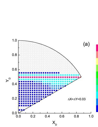
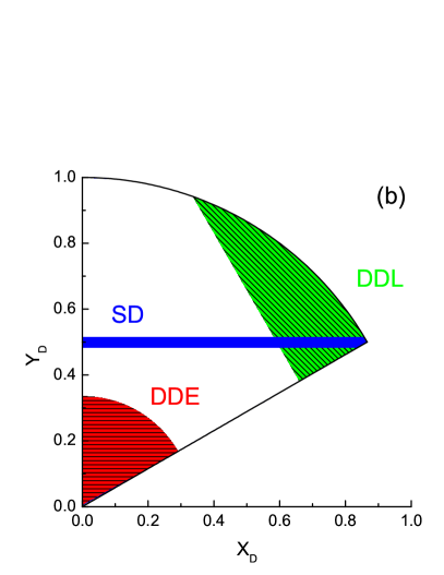
Figure 1: (Color online) (a) The Dalitz plot for the 3-$\alpha$ decay process of the Hoyle state. The number of the events $N(X_{D},Y_{D})$ is plotted for the variables $X_{D}$ and $Y_{D}$ defined in Eq. (17). (b) The kinematical region for the SD, DDL, and DDE, which are described in the text.

Structure of the Hoyle state. The function $\Psi(\boldsymbol{x},\boldsymbol{y})$ at the resonance energy has a concentration of the amplitude at interior region. In Fig. 2, the density distribution

$$\rho(x,y)=x^{2}y^{2}\int d\hat{\boldsymbol{x}}d\hat{\boldsymbol{y}}|\Psi(\boldsymbol{x},\boldsymbol{y})|^{2},$$ (18)

calculated at the Hoyle state energy is plotted. Note that $\Psi(\boldsymbol{x},\boldsymbol{y})$ is not square normalizable, and thus it is artificially normalized within the region, $0\leq x\leq x_{\mathrm{max}}$, and $0\leq y\leq y_{\mathrm{max}}$ with $x_{\mathrm{max}}=y_{\mathrm{max}}=12$ fm. The density has three distinct local peaks denoted by A, B, and C in the figure, which are located at $(x,y)\sim(2.5~{}\mathrm{fm},2.2~{}\mathrm{fm})$, $(3.3~{}\mathrm{fm},4.2~{}\mathrm{fm})$, and $(5.3~{}\mathrm{fm},1.9~{}\mathrm{fm})$, respectively. Similar peak structure is observed in calculations of Refs. Ng13 ; Va12 .

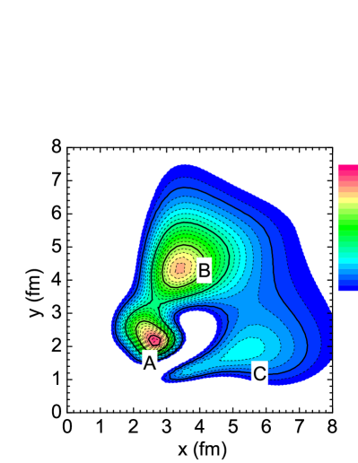
Figure 2: (Color online) Contour plot of the density distribution $\rho(x,y)$ of the Hoyle state.

To reveal the 3-$\alpha$ structure more precisely, I calculate an intrinsic density distribution in a body-fixed frame $\rho_{\mathrm{bf}}(x,y,\Theta)$, where $\Theta$ is the angle between $\hat{\boldsymbol{x}}$ and $\hat{\boldsymbol{y}}$. By defining Euler angles $\boldsymbol{\Omega}$ associated with a rotation to a body-fixed frame ($XYZ$), in which the $Z$-axis is chosen along the vector $\boldsymbol{x}$ and the $XZ$-plane on the plane of 3-$\alpha$, the intrinsic density is calculated as

$$\rho_{\mathrm{bf}}(x,y,\Theta)=x^{2}y^{2}\int d\boldsymbol{\Omega}|\Psi(\boldsymbol{x},\boldsymbol{y})|^{2}.$$ (19)

When two $\alpha$-particles are fixed in a distance $x$, the position of the third $\alpha$-particle on $XZ$-plane is given by $(X,Z)=(y\sin\Theta,y\cos\Theta)$. In Fig. 3, the $\rho_{\mathrm{bf}}(x,y,\Theta)$ densities with fixing $x$ to be the peak positions of $\rho(x,y)$, namely (a) $x=2.5$ fm, (b) 3.3 fm, and (c) 5.5 fm, are plotted. As a reference, an equilateral triangle of side length 2.5 fm is drawn by dashed-line in Fig. 3 (a). Also, isosceles triangles with two equal sides of length 3.3 fm and the third side length being 5.3 fm are drawn in Figs. 3 (b) and (c). The figures show that the peak A corresponds to the configuration of the equilateral triangle, and that the peaks B and C correspond to a bent-arm configuration, in which three $\alpha$-particles compose the isosceles triangle. Because of the symmetric property of the wave function, a bent-arm configuration appears at three points in the density distribution Figs. 3 (b) and (c).

Since each peak is associated with wide slopes, three $\alpha$-particles may take each triangle configuration rather loosely. The probability to find $\alpha$-particles taking the equilateral triangle configuration is estimated by integrating the density $\rho(x,y)$ over a domain of a square, 1.5 fm on a side, around the peak A. This gives about 10 %. Similar procedure for the peak B (C) gives about 20 % (10%). Therefore, the Hoyle state has a mixed configuration of the equilateral triangle with probability 10 % and the bent-arm with 30 %.

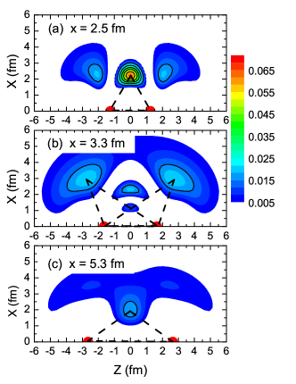
Figure 3: (Color online) Contour plots of the intrinsic density distribution $\rho_{\mathrm{bf}}$ of the Hoyle state for fixed position of two $\alpha$-particles. In figure (a), (b), and (c), two $\alpha$-particles are positioned separating by 2.5 fm, 3.3 fm, and 5.3 fm, respectively. The positions of the two $\alpha$-particles are denoted by the red points in each figure.

Since the Hoyle state is a resonant state, whose wave function does not decay exponentially, observables such as a radius are not well defined. However, because of a resonant character it may simulate a bound state if one restrict the wave function within the interior region where the wave function is normalized. Here, the root mean square radius is calculated by using the following formula,

$$R_{\textrm{rms}}=\sqrt{R_{\alpha}^{2}+\frac{1}{6}\langle x^{2}\rangle+\frac{2}{9}\langle y^{2}\rangle},$$ (20)

where $R_{\alpha}=1.47$ fm, and $\langle x^{2}\rangle$ and $\langle y^{2}\rangle$ are expectation values of $x^{2}$ and $y^{2}$ for the wave function normalized and integrated in the region $0\leq x\leq x_{\mathrm{max}}$ and $0\leq y\leq y_{\mathrm{max}}$. Calculated values of $R_{\textrm{rms}}$ depend on the choice of $x_{\mathrm{max}}$ and $y_{\mathrm{max}}$. It turns out that calculated values of $R_{\textrm{rms}}$ with $x_{\mathrm{max}}=y_{\mathrm{max}}$= 8.0 to 15.0 fm are well fitted by

$$R_{\textrm{rms}}(x_{\mathrm{max}})=3.43-4.87\times 0.70^{x_{\mathrm{max}}},$$ (21)

which gives asymptotically $R_{\textrm{rms}}=$ 3.43 fm. This rather large radius is consistent with calculations given in Refs. Ch07 ; Ka07 .

Summary. Decay modes and the structure of the Hoyle state are studied in the 3-$\alpha$ model by calculating 3-$\alpha$ breakup reactions of the ¹²C$(2_{1}^{+})$ state by the E2 photon. Since little dependence of the results on the choice of $\alpha$-particle interaction models was found, calculations with the Ali-Bodmer-D $\alpha$-$\alpha$ potential together with a 3-$\alpha$ potential are presented. The density distribution at interior region of the Hoyle state has peaks corresponding to the configuration of the equilateral triangle of side length 2.5 fm and that of the isosceles triangle with two equal sides of length 3.3 fm and the third side length being 5.3 fm. The latter corresponds to the bent-arm configuration. Both configurations have wide slopes, which means the Hoyle state is a weak mixture of these configurations. On the other hand, such a structure does not influence the configuration of the outgoing three $\alpha$-particles, which is dominated by the sequential decay process through the ⁸Be$(0_{1}^{+})$. Two-body interaction of two $\alpha$-particles plays an important role when $\alpha$-particles spread.

References

- (1) F. Hoyle, Astrophys. J. Suppl. 1, 121 (1954).
- (2) F. Ajzenberg-Selove, Nucl. Phys. A506, 1 (1990).
- (3) D. R. Tilley, J. H. Kelley, J. L. Godwin, D. J. Millener, J. E. Purcell, C. G. Sheu, and H. R. Weller, Nucl. Phys. A 745, 155 (2004).
- (4) M. Freer, A. H. Wuosmaa, R. R. Betts, D. J. Henderson, P. Wilt, R. W. Zurmühle, D. P. Balamuth, S. Barrow, D. Benton, Q. Li, Z. Liu, and Y. Miao, Phys. Rev. C 49, R1751 (1994).
- (5) J. Manfredi, R. J. Charity, K. Mercurio, R. Shane, L. G. Sobotka, A. H. Wuosmaa, A. Banu, L. Trache, and R. E. Tribble, Phys. Rev. C 85, 037603 (2012).
- (6) O. S. Kirsebom, M. Alcorta, M. J. G. Borge, M. Cubero, C. Aa. Diget, L. M. Fraile, B. R. Fulton, H. O. U. Fynbo, D. Galaviz, B. Jonson, M. Madurga, T. Nilsson, G. Nyman, K. Riisager, O. Tengblad, and M. Turrión, Phys. Rev. Lett. 108, 202501 (2012).
- (7) T. K. Rana, S. Bhattacharya, C. Bhattacharya, S. Kundu, K. Banerjee, T. K. Ghosh, G. Mukherjee, R. Pandey, P. Roy, V. Srivastava, M. Gohil, J. K. Meena, H. Pai, A. K. Saha, J. K. Sahoo, and R. M. Saha, Phys. Rev. C 88, 021601 (2013).
- (8) M. Itoh, S. Ando, T. Aoki, H. Arikawa, S. Ezure, K. Harada, T. Hayamizu, T. Inoue, T. Ishikawa, K. Kato, H. Kawamura, Y. Sakemi, and A. Uchiyama, Phys. Rev. Lett. 113, 102501 (2014).
- (9) C. Angulo, M. Arnould, M. Rayet, P. Descouvemont, D. Baye, C. Leclercq-Willain, A. Coc, S. Barhoumi, P. Aguer, C. Rolfs, R. Kunz, J. W. Hammer, A. Mayer, T. Paradellis, S. Kossionides, C. Chronidou, K. Spyrou, S. Degl’Innocenti, G. Fiorentini, B. Ricci, S. Zavatarelli, C. Providencia, H. Wolters, J. Soares, C. Grama, J. Rahighi, A. Shotter, and M. Lamehi Rachti, Nucl. Phys. A 656, 3 (1999).
- (10) H. Morinaga, Phys. Rev. 101, 254 (1956).
- (11) E. Uegaki, S. Okabe, Y. Abe, and H. Tanaka, Prog. Theor. Phys. 57, 1262 (1977).
- (12) M. Chernykh, H. Feldmeier, T. Neff, P. von Neumann-Cosel, and A. Richter, Phys. Rev. Lett. 98, 032501 (2007).
- (13) E. Epelbaum, H. Krebs, T. A. Lahde, D. Lee, and Ulf-G. Meißner, Phys. Rev. Lett. 109, 252501 (2012).
- (14) Y. Kanada-En’yo, Prog. Theor. Phys. 117, 655 (2007); 121, 895 (2009).
- (15) S. Ishikawa, Phys. Rev. C 87, 055804 (2013).
- (16) L. D. Faddeev, Sov. Phys.-JETP 12, 1041 (1961).
- (17) A. R. Raduta, B. Borderie, E. Geraci, N. Le Neindre, P. Napolitani, M. F. Rivet, R. Alba, F. Amorini, G. Cardella, M. Chatterjee, E. De Filippo, D. Guinet, P. Lautesse, E. La Guidara, G. Lanzalone, G. Lanzano, I. Lombardo, O. Lopez, C. Maiolino, A. Pagano, S. Pirrone, G. Politi, F. Porto, F. Rizzo, P. Russotto, and J. P. Wieleczko, Phys. Lett. B 705, 65 (2011).
- (18) S. Ishikawa, Phys. Rev. C 80, 054002 (2009).
- (19) S. Ali and A. R. Bodmer, Nucl. Phys. 80, 99 (1966).
- (20) D. V. Fedorov and A. S. Jensen, Phys. Lett. B 389, 631 (1996).
- (21) N. B. Nguyen, F. M. Nunes, and I. J. Thompson, Phys. Rev. C 87, 054615 (2013).
- (22) V. Vasilevsky, F. Arickx, W. Vanroose, and J. Broeckhove, Phys. Rev. C 85, 034318 (2012).