Numerical Algorithm for Pólya Enumeration Theorem

Abstract

Although the Pólya enumeration theorem has been used extensively for decades, an optimized, purely numerical algorithm for calculating its coefficients is not readily available. We present such an algorithm for finding the number of unique colorings of a finite set under the action of a finite group.

1 Introduction

A common problem in many fields involves enumerating the possible colorings of a finite set. Applying a symmetry or permutation group reduces the size of the enumerated set by including only those elements that are unique under the group action. The Pólya enumeration theorem counts the number of unique colorings that should be recovered Polya:1987 . The Pólya theorem has shown its wide range of applications in a variety of contexts, such as confirming enumerations of molecules in bioinformatics and chemoinformatics Deng:2014 ; unlabeled, uniform hypergraphs in discrete mathematics Qian:2014 ; and photosensitisers in photosynthesis research Taniguchi:2014 .

Typical implementations of the counting theorem use Computer Algebra Systems to symbolically solve the polynomial coefficient problem. However, despite the widespread use of the theorem, a low-level numerical implementation for recovering the number of unique colorings is not readily available. Although a brute-force calculation of the expansion coefficients for the Pólya polynomial is straight-forward to implement, it is prohibitively slow. For instance, we recently used such a brute force method to confirm enumeration results for a lattice coloring problem in solid state physics Hart:2008 . After profiling performance on more than 20 representative systems, we found that the brute force calculation of the Pólya coefficient took as long as the enumeration problem itself. Here we demonstrate that the performance can be improved drastically by exploiting the properties of polynomials. The improved performance also enables harder Pólya theorem problems to be easily solved that would otherwise be computationally prohibitive .

We first briefly describe the Pólya enumeration theorem in Section 2, followed by the algorithm for calculating the polynomial coefficients in Section 3. In the final Section, we investigate the scaling and performance of the algorithm both heuristically and via numerical experimentation.

2 Pólya Enumeration Theorem

Because of extensive literature coverage, we do not derive the Pólya’s theorem here. Rather, we just state its main claims by using a simple example.

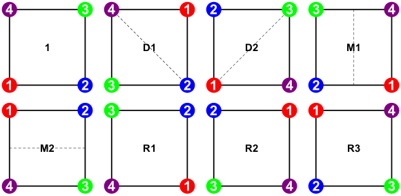
Figure 1: The symmetry group operations of the square. This group is known as the dihedral group of degree 4, or D₄. The dashed lines are guides to the eye for the horizontal, vertical and diagonal reflections (M1,M2 and D1, D2).

The square has the set of symmetries displayed in Figure 1. These symmetries include three rotations (by 90, 180 and 270 degrees; labelled R1, R2, and R3) and four reflections (one horizontal, one vertical and two for the diagonals; labelled M1, M2 and D1, D2). This group is commonly known as the dihedral group of degree four, or D₄ for short.

The group operations of the D₄ group can be written in disjoint-cyclic form as in Table 1. For each $r$-cycle in the group, we can write a polynomial in variables $x_{i}^{r}$ for $i=1\dots\xi$, where $\xi$ is the number of colors used. For this example, we will consider the situation where we want to color the four corners of the square with just two colors. In that case we end up with just two variables $x_{1},x_{2}$, which are represented as $x,y$ in the Table.

Op.	Disjoint-Cyclic	Polynomial	Expanded	Coeff.
$\mathbb{1}$	$(1)(2)(3)(4)$	$(x+y)^{4}$	$x^{4}+4x^{3}y+6x^{2}y^{2}+4xy^{3}+y^{4}$	6
D1	$(1,3)(2)(4)$	$(x^{2}+y^{2})(x+y)^{2}$	$x^{4}+2x^{3}y+2x^{2}y^{2}+2xy^{3}+y^{4}$	2
D2	$(1,2)(3)(4)$	$(x^{2}+y^{2})(x+y)^{2}$	$x^{4}+2x^{3}y+2x^{2}y^{2}+2xy^{3}+y^{4}$	2
M1	$(1,2)(3,4)$	$(x^{2}+y^{2})^{2}$	$x^{4}+2x^{2}y^{2}+y^{4}$	2
M2	$(1,4)(2,3)$	$(x^{2}+y^{2})^{2}$	$x^{4}+2x^{2}y^{2}+y^{4}$	2
R1	$(1,4,3,2)$	$(x^{4}+y^{4})$	$x^{4}+y^{4}$	0
R2	$(1,3)(2,4)$	$(x^{2}+y^{2})^{2}$	$x^{4}+2x^{2}y^{2}+y^{4}$	2
R3	$(1,2,3,4)$	$(x^{4}+y^{4})$	$x^{4}+y^{4}$	0

Table 1: Disjoint-cyclic form for each group operation in D₄ and the corresponding polynomials, expanded polynomials and the coefficient of the $x^{2}y^{2}$ term for each.

The Pólya representation for a single group operation in disjoint-cyclic form results in a product of polynomials that we can expand. For example, the group operation D1 has disjoint-cyclic form $(1,3)(2)(4)$ that can be represented by the polynomial $(x^{2}+y^{2})(x+y)(x+y)$ where the exponent on each variable corresponds to the length of the $r$-cycle that it is part of. For a general $r$-cycle, the polynomial takes the form

$$(x_{1}^{r}+x_{2}^{r}+\cdots+x_{\xi}^{r}),$$ (1)

for an enumeration with $\xi$ colors. Most group operations will have a product of these polynomials for each $r$-cycle in the disjoint-cyclic form. Once the product of polynomials has been generated with the group operation, we can simplify it by adding exponents to identical polynomials. In the example above, $(x+y)(x+y)$ would become $(x+y)^{2}$; in summary, we exchange the group operations acting on the set for polynomial representations that obey the familiar rules for polynomials.

We will now pursue our example of the possible colorings on the four corners of the square involving two of each color. Excluding the symmetry operations, we could come up with ${4\choose 2}=6$ possibilities, but some of these are equivalent by symmetry. The Pólya theorem will count how many unique colorings we should recover. To find out the expected number of unique colorings, we look at the coefficient of the term corresponding to the overall color selection (in this example, two of each color); thus we look for coefficients of the $x^{2}y^{2}$ term for each group operation. These coefficient values are listed in Table 1. The sum of these coefficients, divided by the number of operations in the group, gives the total number of unique colorings under the entire group action, in this case $(6+2+2+2+2+0+2+0)/8=16/8=2$. The unique colorings are plotted in Figure 2.

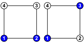
Figure 2: The two unique ways to color the square with two colors and two corners of each color.

Generally, for a finite set with $F$ elements, and fixed color concentrations $c_{i}$ such that $\sum_{i=1}^{\xi}c_{i}=F$, the number of unique colorings of the set under the group action corresponds to the coefficient of the term

$$T=x_{1}^{c_{1}}x_{2}^{c_{2}}\dots x_{\xi}^{c_{\xi}}=\prod_{i}^{\xi}x_{i}^{c_{i}}$$ (2)

in the expanded polynomial for each group operation, summed over all elements in the group. Counting the number of unique colorings at fixed concentration amounts to finding the coefficient of a specific term, known a priori, from a product of polynomials.

3 Coefficient-Finding Algorithm

We begin by reviewing some well-known properties of polynomials with respect to their variables. First, for a generic polynomial

$$(x_{1}^{r}+x_{2}^{r}+\cdots+x_{\xi}^{r})^{d},$$ (3)

the exponents of each $x_{i}$ in the expanded polynomial are constrained to the set

$$V=\{0,r,2r,3r,\dots,dr\}.$$ (4)

Next, we consider the terms in the expansion of the polynomial:

$$(x_{1}^{r}+x_{2}^{r}+\cdots+x_{\xi}^{r})^{d}=\sum_{k_{1},k_{2},\dots,k_{\xi}}\mu_{k}\prod_{i=1}^{\xi}x_{i}^{rk_{i}}$$ (5)

where the sum is over all possibles sequences $k_{1},k_{2},\dots,k_{\xi}$ such that the sum of the exponents (represented by the sequence in $k_{i}$) is equal to $d$,

$$k_{1}+k_{2}+\cdots+k_{\xi}=d.$$ (6)

The coefficients $\mu_{k}$ in the polynomial expansion Equation (5) are found using the multinomial tcoefficients

$$\mu_{k} = {n\choose{k_{1},k_{2},\dots,k_{\xi}}}=\frac{n!}{k_{1}!k_{2}!\cdots k_{\xi}!}$$ (7)

$$= {{k_{1}}\choose{k_{1}}}{{k_{1}+k_{2}}\choose{k_{2}}}\cdots{{k_{1}+k_{2}+\cdots+k_{\xi}}\choose{k_{\xi}}}$$

$$= \prod_{i=1}^{\xi}{{\sum_{j=1}^{i}k_{j}}\choose k_{i}}.$$

Finally, we define the polynomial (1) for an arbitrary group operation $G^{i}\in\bf{G}$ as

$$P^{i}(x_{1},x_{2},\dots,x_{\xi})=\prod_{\alpha=1}^{m}M_{\alpha}^{r_{\alpha}}(x_{1},x_{2},\dots,x_{\xi})$$ (8)

where each $M_{\alpha}^{r_{\alpha}}$ is a polynomial for the $\alpha^{\mathrm{th}}$ distinct $r$-cycle of the form (3) and $d_{\alpha}$ is substituted for the value of $d$ (which is the multiplicity of that $r$-cycle); $m$ is the number of distinct values of $r_{\alpha}$ in $P^{i}$.

Since we know the fixed concentration term $T=\prod_{i=1}^{\xi}T_{i}=\prod_{i=1}^{\xi}x_{i}^{c_{i}}$ in advance (see equation (2)), we can limit the possible sequences of $k_{i}$ for which multinomial coefficients are calculated. This is the key idea of the algorithm and the reason for its high performance.

For each group operation $G^{i}$, we have a product of polynomials $M_{\alpha}^{r_{\alpha}}$. We begin filtering the sequences by choosing only those combinations of values $v_{i\alpha}\in V_{\alpha}=\{v_{i\alpha}\}_{i=1}^{d_{\alpha}+1}$ for which the sum

$$\sum_{\alpha=1}^{m}v_{i\alpha}=T_{i}$$ (9)

where $V_{\alpha}$ is the set from eqn. (4) for multinomial $M_{\alpha}^{r_{\alpha}}$.

We first apply constraint (9) to the $x_{1}$ term across the product of polynomials to find a set of values $\{k_{1\alpha}\}_{\alpha=1}^{m}$ that could give exponent $T_{1}$ once all the polynomials’ terms have been expanded. Once a value $k_{1\alpha}$ has been fixed for each $M_{\alpha}^{r_{\alpha}}$, the remaining exponents in the sequence $\{k_{1\alpha}\}\cup\{k_{i\alpha}\}_{i=2}^{\xi}$ are constrained via (6). We can recursively examine each variable $x_{i}$ in turn using these constraints to build a set of sequences

$$S_{l}=\{S_{l\alpha}\}_{\alpha=1}^{m}=\{(k_{1\alpha},k_{2\alpha},\dots,k_{\xi\alpha})\}_{\alpha=1}^{m}$$ (10)

where each $S_{l\alpha}$ defines the exponent sequence for its polynomial $M_{\alpha}^{r_{\alpha}}$ that will produce the target term $T$ after the product is expanded. The maximum value of $l$ depends on the target term $T$ and how many possible $v_{i\alpha}$ values are filtered out using constraints (9) and (6) at each step in the recursion.

Once the set ${\bf S}=\{S_{l}\}$ has been constructed, we use Equation (7) on each polynomial’s $\{k_{i\alpha}\}_{i=1}^{\xi}$ in $S_{l\alpha}$ to find the contributing coefficients. The final coefficient value for term $T$ resulting from operation $G^{i}$ is

$$t_{i}=\sum_{l}\tau_{l}=\sum_{l}\prod_{\alpha=1}^{m}{d_{\alpha}\choose S_{l\alpha}}.$$ (11)

To find the total number of unique colorings under the group action, this process is applied to each element $G^{i}\in{\bf G}$ and the results are summed and then divided by $|{\bf G}|$.

We can further optimize the search for contributing terms by ordering the exponents in the target term $T$ in descending order. Because the possible sequences $\{k_{1\alpha}\}_{\alpha=1}^{m}$ are filtered using $T_{1}$, larger values for $T_{1}$ are more likely to result in smaller sets of $\{k_{i\alpha}\}_{\alpha=1}^{m}$ across the polynomials. All the $\{k_{1\alpha}\}_{\alpha=1}^{m}$ need to sum to $T_{1}$ (9); if $T_{1}$ has smaller values (like 1 or 2), we will end up with lots of possible ways to arrange them to sum to $T_{1}$ (which is not the the case for the larger values). Since the final set of sequences $S_{l}$ is formed using a cartesian product, having a few extra sequences from the $T_{1}$ pruning multiplies the total number of sequences significantly. Additionally, constraint (6) applied within each polynomial will also reduce the total number of sequences to consider if the first variables $x_{1},x_{2}$, etc. are larger integers.

3.1 Pseudocode Implementation

Note. Implementations in python and Fortran are available in the supplementary material.

For both algorithms presented below, the operator ($\Leftarrow$) pushes the value to its right onto the list to its left.

Algorithm 1 Recursive Sequence Constructor

procedure initialize($i$, $k_{i\alpha}$, $M_{\alpha}^{r_{\alpha}}$, $V_{\alpha}$, ${\bf T}$)

     Constructs a Sequence Object tree recursively for a

     single $M_{\alpha}^{r_{\alpha}}$ by filtering possible exponents on each $x_{i}$

     in the polynomial. The object has the following

     properties:

       root: $k_{i\alpha}$, proposed exponent of variable $x_{i}$ in $M_{\alpha}^{r_{\alpha}}$.

       parent: proposed Sequence object for $k_{i-1,\alpha}$ of $x_{i-1}$.

       used: the sum of the proposed exponents to left of

              and including this variable $\sum_{j=1}^{i}k_{i\alpha}$.

     

     $i$: index of variable in $M_{\alpha}^{r_{\alpha}}$

     $k_{i\alpha}$: proposed exponent of variable $x_{i}$ in $M_{\alpha}^{r_{\alpha}}$.

     $M_{\alpha}^{r_{\alpha}}$: Pólya polynomial representation of a single

             polynomial in $P^{i}$ (8).

     $V_{\alpha}$: possible exponents for $M_{\alpha}^{r_{\alpha}}$ (4).

     ${\bf T}$: $\{T_{i}\}_{i=1}^{\xi}$ exponents for the concentration term (2).

     

     if $i=1$ then

         self.used $\leftarrow$ self.root + self.parent.used

     else

         self.used $\leftarrow$ self.root      

     self.kids $\leftarrow$ empty

     if $i\leq\xi$ then

         for $p\in V_{\alpha}$ do

              $rem\leftarrow$ $p$ - self.root

              if $0\leq rem\leq T_{i}$ and $|rem|\leq d_{\alpha}r_{\alpha}-\textit{self}.\textrm{used}$

               and $|p-\textit{self}.\textrm{used}|\,\textrm{mod}\,r_{\alpha}=0$ then

                  $\textit{self}.\textrm{kids}\Leftarrow\textrm{Sequence}(i+1,rem,M_{\alpha}^{r_{\alpha}},V_{\alpha},{\bf T})$                             

function expand(sequence)

     Generates a set of $S_{l\alpha}$ from a single Sequence object.

     sequence: the object created using initialize.

     

     $\textit{sequences}\leftarrow$ empty

     for $\textit{kid}\in$ sequence.kids do

         for $\textit{seq}\in\textsc{expand}(kid)$ do

              $\textit{sequences}\Leftarrow kid.\textrm{root}\cup\textit{seq}$               

     if $\textrm{len(sequence.kids)}=0$ then

         $\textit{sequences}\leftarrow\{kid.\textrm{root}\}$      

     return sequences

function build_S_l(${\bf k}$, ${\bf V}$, $P^{i}$, ${\bf T}$)

     Constructs $S_{l}$ from $\{k_{1\alpha}\}_{\alpha=1}^{m}$ for a $P^{i}$ (8).

     ${\bf k}$: $\{k_{1\alpha}\}_{\alpha=1}^{m}$ set of possible exponent values on the

         first variable in each $M_{\alpha}^{r_{\alpha}}\in P^{i}$.

     ${\bf V}$: $\{V_{\alpha}\}_{\alpha=1}^{m}$ possible exponents for each $M_{\alpha}^{r_{\alpha}}$ (4).

     $P^{i}$: Pólya polynomial representation for a single

           operation in the group ${\bf G}$ (8).

     ${\bf T}$: $\{T_{i}\}_{i=1}^{\xi}$ exponents for the concentration term (2).

     

     $\textit{sequences}\leftarrow\textrm{empty}$

     for $\alpha\in\{1\dots m\}$ do

         $\textit{seq}\leftarrow\textsc{initialize}(1,k_{1\alpha},M_{\alpha}^{r_{\alpha}},V_{\alpha},{\bf T})$

         $\textit{sequences}\Leftarrow\textsc{expand}(seq)$      

     return sequences

For algorithm (1) in the expand procedure, the $\cup$ operator horizontally concatenates the integer root to an existing sequence of integers.

For build_S_l, we use the exponent $k_{1\alpha}$ on the first variable in each polynomial to construct a full set of possible sequences for that polynomial. Those sets of sequences are then combined in sum_sequences (alg. 2) using a cartesian product over the sets in each multinomial.

Algorithm 2 Coefficient Calculator

function sum_sequences(S_l)

     Finds $\tau_{l}$ (11) for $S_{l}=\{S_{l\alpha}\}_{\alpha=1}^{m}$ (10)

     S_l: a set of lists (of exponent sequences $\{k_{i\alpha}\}_{i=1}^{\xi}$)

         for each polynomial $M_{\alpha}^{r_{\alpha}}$ in the product $P^{i}$ (8).

     

     $K_{l}\leftarrow S_{l1}\times S_{l2}\times\dots\times S_{lm}=\langle\{(k_{i\alpha})_{i=1}^{\xi}\}_{\alpha=1}^{m}\rangle_{l}$

     $\textit{coeff}\leftarrow 0$

     for each $\{(k_{i\alpha})_{i=1}^{\xi}\}_{\alpha=1}^{m}\in K_{l}$ do

         if $\sum_{\alpha=1}^{m}k_{i\alpha}=T_{i}\;\forall\;i\in\{1\dots\xi\}$ then

              $\textit{coeff}\leftarrow\textit{coeff}+\prod_{\alpha=1}^{m}{d_{\alpha}\choose\{k_{i\alpha}\}_{i=1}^{\xi}}$               

     return coeff

function coefficient(${\bf T}$, $P^{i}$, ${\bf V}$)

     Constructs ${\bf S}=\{S_{l}\}$ and calculates $t_{i}$ (11)

     ${\bf T}$: $\{T_{i}\}_{i=1}^{\xi}$ exponents for the concentration term (2).

     $P^{i}$: Pólya polynomial representation for a single

           operation in the group ${\bf G}$ (8).

     ${\bf V}$: $\{V_{\alpha}\}_{\alpha=1}^{m}$ possible exponents for each $M_{\alpha}^{r_{\alpha}}$ (4).

     

     if $m=1$ then

         if $r_{1}>T_{i}\;\forall\;i=1..\xi$ then

              return $0$

         else

              return ${d_{1}\choose{T_{1}T_{2}\dots T_{\xi}}}$          

     else

         ${\bf T}\leftarrow\textrm{sorted}({\bf T})$

         $\textit{possible}\leftarrow V_{1}\times V_{2}\times\dots\times V_{m}$

         $\textit{coeffs}\leftarrow 0$

         for $\{k_{1\alpha}\}_{\alpha=1}^{m}\in\textit{possible}$ do

              if $\sum_{\alpha=1}^{m}k_{1\alpha}=T_{1}$ then

                  $S_{l}\leftarrow\textsc{build\_S}_{l}(\{k_{1\alpha}\}_{\alpha=1}^{m},{\bf V},P^{i},{\bf T})$

                  $\textit{coeffs}\leftarrow\textit{coeffs}+\textsc{sum\_sequences}(S_{l})$                        

         return coeffs      

For algorithm (2) in the sum_sequences function, $K_{l}$ is calculated using the cartesian product of the individual $S_{l\alpha}$, where for a given $l$, the number of sequences $\{k_{i}\}_{i=1}^{\xi}\in S_{l\alpha}$ may be arbitrary. For example, a product of three polynomials $M_{1}^{4}M_{2}^{3}M_{3}^{2}$ may produce possible sequences with $|S_{l1}|=2$, $|S_{l2}|=4$ and $|S_{l3}|=4$. Then $|K_{l}|=2\times 4\times 4=32$ and each element in $K_{l}$ is a set of three sequences: $\{(k_{i\alpha})_{i=1}^{\xi}\}_{\alpha=1}^{3}$, one for each polynomial, which specifies the exponents on the contributing term from that polynomial. Also, when calculating multinomial coefficients, we use the form in eqn. (7) in terms of binomial coefficients with a fast, stable algorithm from Manolopoulos Manolo2002 .

In practice, many of the group operations $G^{i}$ produce identical products $M_{1}^{r_{1}}M_{2}^{r_{2}}\dots M_{m}^{r_{m}}$. Thus before computing any of the coefficients from the polynomials, we first form the polynomial products for each group operation and then add identical products together.

4 Computational Order and Performance

The algorithm is structured around the a priori knowledge of the fixed concentration term (2). At the earliest possibility, we prune terms from individual polynomials that would not contribute to the final polya coefficient in the expanded product of polynomials. Because the Pólya polynomial for each group operation is based on its disjoint-cyclic form, the complexity of the search can vary drastically from one group operation to the next. That said, it is common for groups to have several classes whose group operations (within each class) will have similar disjoint-cyclic forms and thus also scale similarly. However, from group to group, the set of classes and disjoint-cyclic forms may be very different; this makes it difficult to make a statement about the scaling of the algorithm in general. Although we could make statements about the scaling of well-known sets of groups (for example the dihedral groups used in our example above), we decided instead to craft certain special groups with specific properties and run tests to determine the scaling numerically.

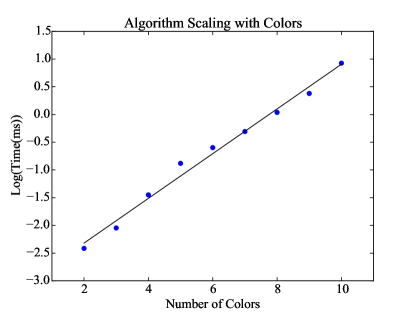
Figure 3: Log plot of the algorithm scaling as the number of colors increases. Since the number of variables $x_{i}$ in each polynomial increases with the number of colors, the combinatoric complexity of the expanded polynomial increases drastically with each additional color; this leads to an exponential scaling. The linear fit to the logarithmic data has a slope of 0.403.

In Figure 3 we plot the algorithm’s scaling as the number of colors in the enumeration increases. For each $r$-cycle in the disjoint-cyclic form of a group operation, we construct a polynomial with $\xi$ variables, where $\xi$ is the number of colors used in the enumeration. Because the group operation results in a product of these polynomials, increasing the number of colors by 1 increases the combinatoric complexity of the polynomial expansion exponentially. For this scaling experiment, we used the same transitive group acting on a finite set with 20 elements for each data point, but increased the number of colors in the fixed color term $T$. We chose $T$ by dividing the number of elements in the group as equally as possible; thus for 2 colors, we used $[10,10]$; for 3 colors we used $[8,6,6]$, then $[5,5,5,5]$, $[4,4,4,4,4]$, etc. Figure 3 plots the $\log_{10}$ of the execution time (in ms) as the number of colors increases. As expected, the scaling is linear (on the log plot). The linear fit to the data points has a slope of $0.403$.

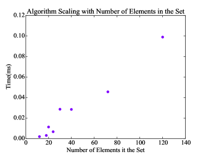
Figure 4: Algorithm scaling as the number of elements in the finite set increases. The Pólya polynomial arises from the group operations’ disjoint-cyclic form, so that more elements in the set results in a richer spectrum of possible polynomials multiplied together. Because of the algorithms aggresive pruning of terms, the exact disjoint-cyclic form of individual group operations has a large bearing on the algorithm’s scaling. As such it isn’t surprising that there is some scatter in the timings as the number of elements in the set increases.

As the number of elements in the finite set increases, the possible Pólya polynomial representations for each group operation’s disjoint-cyclic form increases exponentially. In the worst case, a group acting on a set with $k$ elements may have an operation with $k$ 1-cycles; on the other hand, that same group may have an operation with a single $k$-cycle, with lots of possibilities in between. Because of the richness of possibilities, it is almost impossible to make general statements about the algorithm’s scaling without knowing the structure of the group and its classes. In Figure 4, we plot the scaling for a set of related groups (all are isomorphic to the direct product of S₃ $\times$ S₄) applied to finite sets of varying sizes. Every data point was generated using a transitive group with 144 elements. Thus, this plot shows the algorithm’s scaling when the group is the same and the number of elements in the finite set changes. Although the scaling appears almost linear, there is a lot of scatter in the data. Given the rich spectrum of possible Pólya polynomials that we can form as the set size increases, the scatter isn’t surprising.

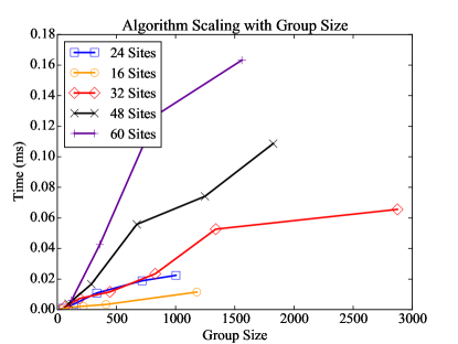
Figure 5: Algorithm scaling with group size for an enumeration problem from solid state physics Hart:2008 . We used the unique permutation groups arising from all derivative super structures of a simple cubic lattice for a given number of sites in the unit cell. The behavior is generally linear with increasing group size.

Finally, we consider the scaling as the group size increases. For this test, we selected the set of unique groups arising from the enumeration of all derivative super structures of a simple cubic lattice for a given number of sites in the unit cell Hart:2008 . Since the groups are formed from the symmetries of real crystals, they arise from the semidirect product of operations related to physical rotations and translations of the crystal. In this respect, they have similar structure for comparison. In most cases, the scaling is obviously linear; however, the slope of each trend varies from group to group. This once again highlights the scaling’s heavy dependence on the specific disjoint-cyclic forms of the group operations. Even for groups with obvious similarity, the scaling may be different.

5 Summary

Until now, no low-level, numerical implementation of Pólya’s enumeration theorem was readily available; instead, a computer algebra system (CAS) was used to symbolically solve the polynomial expansion problem posed by Pólya. While such systems are effective for small, simpler calculations, as the difficulty of the problem increases, they become impractical solutions. Additionally, codes that perform the actual enumeration of the colorings are often implemented in low-level codes and interoperability with a CAS is not necessarily easy to automate.

We presented a low-level, purely numerical algorithm that exploits the properties of polynomials to restrict the combinatoric complexity of the expansion. By considering only those coefficients in the unexpanded polynomials that might contribute to the final answer, the algorithm reduces the number of terms that must be included to find the significant term in the expansion.

Because of the algorithm scaling’s reliance on the exact structure of the group and the disjoint-cyclic form of its operations, a rigorous analysis of the scaling is not possible without knowledge of the group. Instead, we presented some numerical timing results from representative, real-life problems that show the general scaling behavior. Because all the timings are in the millisecond to second regime anyway, a more rigorous analysis of the algorithm’s scaling is unnecessary.

In contrast to the CAS solutions whose execution times range from milliseconds to hours, our algorithm consistently performs in the millisecond to second regime, even for complex problems. Additionally, it is easy to implement in low-level languages, making it useful for confirming enumeration results. This makes it an effective substitute for alternative CAS implementations.

In computational materials science, chemistry, and related subfields such as computational drug discovery, combinatorial searches are becoming increasingly important, especially in high-throughput studies nmat_review . The upside potential of these efforts continues to grow because computing power continues to become cheaper and algorithms continue to evolve. As computational methods gain a larger market share in materials discovery, algorithms such as this one are important as they provide validation support to complex simulation codes. The present algorithm has been useful in checking a new algorithm extending the work in Refs. Hart:2008 ; Hart:2009 ; Hart:2012 , and Pólya’s theorem was recently used in Mustapha’s enumeration algorithmMustapha:2013 that has been incorporated into the CRYSTAL14 software package QUA:QUA24658 .

6 Supplementary Material

The source code to implement this algorithm is available for both python and Fortran at:

https://github.com/rosenbrockc/polya

The home page on github has full instructions for using either version of the code as well a battery of over 50 unit tests that were used to verify and time the algorithm. The unit tests can be executed using the fortpy framework available via the Python Package Index. Instructions for running the unit tests are also on the github home page.