On regularizations of the Dirac delta distribution

Abstract

In this article we consider regularizations of the Dirac delta distribution with applications to prototypical elliptic and hyperbolic partial differential equations (PDEs). We study the convergence of a sequence of distributions $\mathcal{S}_{H}$ to a singular term $\mathcal{S}$ as a parameter $H$ (associated with the support size of $\mathcal{S}_{H}$) shrinks to zero. We characterize this convergence in both the weak-$\ast$ topology of distributions, as well as in a weighted Sobolev norm. These notions motivate a framework for constructing regularizations of the delta distribution that includes a large class of existing methods in the literature. This framework allows different regularizations to be compared. The convergence of solutions of PDEs with these regularized source terms is then studied in various topologies such as pointwise convergence on a deleted neighborhood and weighted Sobolev norms. We also examine the lack of symmetry in tensor product regularizations and effects of dissipative error in hyperbolic problems.

1 Introduction

Many phenomena in the physical sciences are modelled by partial differential equations (PDE) with singular source terms. The solutions of such PDE models are often studied using numerical approximations. In some computational approaches, the singular source terms are represented exactly, such as in [1, 7, 8, 35]. A more common approach is to approximate the source term using some regularized function, and then obtain the numerical solution using a discretization of the PDE with the approximate source. One prominent example of the utility of singular sources in applications is the immersed boundary method [28], wherein a Dirac delta distribution supported on an immersed fiber or surface is used to capture the two-way interaction between a dynamically evolving elastic membrane and the incompressible fluid in which it is immersed. In immersed boundary simulations, the Dirac delta is replaced by a continuous approximation that is designed to satisfy a number of constraints that guarantee certain desirable properties of the analytical and numerical solution. Related approximations are also employed in connection with the level set method [27] and vortex methods [3, 10].

Suppose we represent the original problem of interest in an abstract form as follows:

1. Find $u$ such that

   $$\mathcal{L}(u)=\mathcal{S},$$ (1a)

   where $\mathcal{L}$ is a PDE operator and $\mathcal{S}$ is a distribution which is used to model a singular source.

Then let $\mathcal{S}_{H}$ denote some approximation of $\mathcal{S}$ and consider the associated problem

1. Find $u_{H}$ such that

   $$\mathcal{L}(u_{H})=\mathcal{S}_{H}.$$ (1b)

Here, $H>0$ is some small parameter for which $\mathcal{S}_{H}\rightarrow\mathcal{S}$ in some sense as $H\rightarrow 0$ (a sense that will be made concrete later on). One may then apply an appropriate numerical scheme (e.g., finite difference, finite volume, finite element, spectral, etc.) with a discretization parameter $h>0$, thereby obtaining two discrete solution approximations: $u_{h}$ to $u$ in Problem 1; and $u_{H,h}$ to $u_{H}$ in Problem 2. We are free, of course, to pick one numerical scheme for Problem 1 and a different scheme for Problem 2. If the numerical schemes are suitably well-chosen, then both $u_{h}\rightarrow u$ and $u_{H,h}\rightarrow u_{H}$ as $h\rightarrow 0$.

In practical computations, it may not be possible to construct $u_{h}$. Indeed, it is typically only $u_{H,h}$ that is computed, by first prescribing some approximation to the source term and then discretizing the PDE with the approximate source. Ideally, what we hope to obtain is that as both $h,H\rightarrow 0$, the discrete approximant $u_{H,h}\approx u$. In the immersed boundary method, for example, the source term $\mathcal{S}$ is a line source and both the approximation of the source term and the discretization of the PDE are performed with reference to the same underlying spatial grid, so that parameters $H$ and $h$ are identical. Convergence of $u_{H,h}\to u$ in the context of the immersed boundary method has been the subject of detailed analysis in the works of Liu and Mori [23, 24, 26]. However, these authors only focus on convergence of the discrete regularizations and do not consider $u_{H}\to u$.

In this article we are concerned primarily with two questions:

1. How do we construct ‘good’ approximations $\mathcal{S}_{H}$ to $\mathcal{S}$?

2. How does the choice of approximation $\mathcal{S}_{H}$ affect the the convergence of $u_{H,h}\rightarrow u$?

Before we can formulate answers to the above, we have to first answer the two related questions:

1. What form of convergence should be used to examine $\mathcal{S}_{H}\rightarrow\mathcal{S}$?

2. What form of convergence should be used to examine $u_{H,h}\rightarrow u$?

In this paper, we restrict our attention to the particular case of $\mathcal{S}=\delta$ which denotes the well-known point source distribution (or Dirac delta distribution) having support at the origin.

Questions 1 and 2 are fairly well-studied in some contexts [16, 23, 24, 6, 32, 31, 30, 36] but Questions 3 and 4 have not been the subject of much scrutiny in the literature. A common approach for approximating $\mathcal{S}_{H}$ (via regularization) is to construct a discrete regularization that is tailored to specific quadrature methods. Waldén [34] presents an analysis of discrete approximations of the delta distribution, restricting his attention to applications to PDEs in one dimension. Tornberg and Engquist [32] analyze discrete approximations to the delta distribution in multiple dimensions with compact support and draw a connection between the discrete moment conditions and the order of convergence of the solution of a PDE with the discrete $\mathcal{S}_{H}$ as source term. They also consider approximations of line sources using a singular source term or a collection of delta distributions in a chain. The analyses of Tornberg [30] and Tornberg and Engquist [31] for the discrete approximations $\mathcal{S}_{H}$ rely on the choice of mesh and quadrature rules. They also restrict $H=\mathcal{O}(h)$ and compare $u_{H,h}$ directly to $u$ so that, $\mathcal{S}_{H}$ is de based on the numerical method used to compute $u_{H,h}$. More recently, Suarez et al. [29] considered regularizations of the delta distribution that are tailored to spectral collocation methods for the solution of hyperbolic conservation laws. Their approach to constructing polynomial regularizations using the Chebyshev basis has a similar flavor to our approach, as will be seen in Section 3. In a different approach, Benvenuti et al. [5] study the case of regularizations that are not compactly supported but have rapidly decaying Fourier transforms in the context of extended finite element methods (XFEM) [4]. The authors demonstrate that such regularizations lead to lower numerical errors since they can be integrated using common quadrature methods such as Gauss quadrature.

In this article we demonstrate firstly how to develop regularizations $\mathcal{S}_{H}$ independent of the choice of numerical discretization. For example, in answering Question 1 we derive piecewise smooth approximations $\mathcal{S}_{H}$. We can then examine the intermediate errors $\|u-u_{H}\|_{X}$ and $\|u_{H}-u_{H,h}\|_{X}$ and use the triangle inequality to give a bound on

$$\|u-u_{H,h}\|_{X}\leq\underbrace{\|u-u_{H}\|_{X}}_{\mbox{\footnotesize regularization error}}+\underbrace{\|u_{H}-u_{H,h}\|_{X}}_{\mbox{\footnotesize discretization error}},$$ (2)

where $\|\cdot\|_{X}$ refers to a suitably chosen norm; the choice of norms is discussed below. For fixed $H>0$ the discretization errors $\|u_{H,h}-u_{H}\|_{X}$ are analyzed using properties of the numerical scheme and regularity of solutions of Problem 2. The resulting discretization errors are well-understood for specific problems and specific schemes, and so we focus our attention here on the regularization errors.

We propose a unified approach for construction and analysis of regularizations. This has three advantages: First, we are able to provide a simple strategy for constructing new regularizations suitable for a given application (and not constrained to a specific numerical method for that application). Second, our framework is flexible and allows us to study the effect of additional constraints on the regularizations. For example, it is common in the immersed boundary method to impose the even-odd conditions on the discrete regularizations, but the effect of these conditions on the regularization error is subtle [26]. Third, our framework provides a unified platform from which to compare different regularizations in the literature. For example, in Section 3 we show that both radially symmetric and tensor product regularizations lead to the same regularization errors, but their discretization errors may differ. This provides more insight into the result of [32] indicating that regularizations based on distance functions can lead to large errors. Our results indicate that this is due to the discretization error and not the regularization error. An important point to note is that we do not account for errors due to the use of discrete quadrature rules; these are embedded in the analysis of the discretization errors, and our goal is instead to examine the errors purely due to regularization.

The construction procedure requires us to first obtain answers to Questions 3 and 4. The mode of convergence and (where appropriate) the norm $\|\cdot\|_{X}$ are chosen in a problem-dependent manner. More precisely, if we seek approximations of solutions to Problem 1 in some Hilbert space $\mathcal{H}$, and if the PDE operator $\mathcal{L}:\mathcal{H}\rightarrow\mathcal{H}^{*}$, then we need a strategy to construct regularizations $\mathcal{S}_{H}$ from suitable elements in $\mathcal{H}^{\ast}$ so that $u_{H}$ converges to $u$ in $\mathcal{H}$.

We begin by constructing linear functionals $\tilde{\delta}_{H}$ via smooth and compactly supported elements of $\mathcal{H}$. We then discuss the convergence of $\tilde{\delta}_{H}\to\delta$ in the weak-$\ast$ topology and in a class of weighted Sobolev norms. Then we derive a set of continuous moment conditions that are entirely analogous to the discrete moment conditions of [32]. A strategy for solving a finite number of moment equations is presented using a basis of our choice, after which we consider convergence of $u_{H}\to u$ in the sup-norm in a deleted neighbourhood and a different class of weighted Sobolev norms for some operators $\mathcal{L}$.

We emphasize that in this article our focus is on regularizations that have compact support. However, some of our results such as the moment conditions of Definition 3 can be readily generalized to the case of regularizations that are not compactly supported. We also note that in general, the continuous regularizations we construct are not unique. In the specific case where Legendre polynomials are chosen as a basis while solving the moment problem, the continuous regularizations are polynomials on the support of $\delta_{H}\in\mathcal{H}$. These $\delta_{H}$ can then be made to have arbitrary smoothness by adding extra continuity conditions; this should be compared with the piecewise polynomial approximants that are obtained using discrete regularizations.

In most applications of interest, the domains on which we numerically compute our approximate PDE solutions are polygonal. We also focus on PDE operators $\mathcal{L}$ associated with free space or zero Dirichlet boundary data, although our analysis and solution construction are easily extended to more general cases.

The framework we present in this paper is independent of the specific choice of numerical method used to approximate solutions of the regularized problem. To this end, we present computations using spectral and finite element methods within readily-available implementations.

Throughout the remainder of this paper, $\Omega$ will represent an open Lipschitz domain in $\mathbb{R}^{n}$ with polygonal boundary that contains the origin.

2 Background

We begin by fixing notation. We denote the set of test functions by $\mathcal{D}(\Omega)$. This is the space of real-valued $C^{\infty}$ functions that are compactly supported in $\Omega$ and equipped with the usual topology of the test functions. We denote the distributions by $\mathcal{D}^{\ast}(\Omega)$, the dual of $\mathcal{D}(\Omega)$. The point source or delta distribution $\delta\in\mathcal{D}^{\ast}(\Omega)$ (also called the Dirac delta functional) is defined by

$$\delta(\phi):=\phi(0)\quad\text{ for }\phi\in\mathcal{D}(\Omega).$$

A natural setting in which to study solutions of Problem 1 is in a Sobolev space $\mathcal{H}_{0}^{s}(\Omega)$ for $s\in\mathbb{R}$ and $s>0$. The particular choice of $s$ is dictated by the differential operator $\mathcal{L}$. Since $\mathcal{H}_{0}^{s}(\Omega)$ is a Hilbert space, and since the continuous inclusion map from $\mathcal{D}(\Omega)\rightarrow\mathcal{H}_{0}^{s}(\Omega)$ is dense, the spaces $(\mathcal{D}(\Omega),\mathcal{H}_{0}^{s}(\Omega),\mathcal{D}^{\ast}(\Omega))$ form a Gel’fand triple (see [20]). This means that we can identify the dual of $\mathcal{H}^{s}_{0}(\Omega)$ with elements of $\mathcal{D}^{\ast}(\Omega)$, i.e. $(\mathcal{H}^{s}_{0})^{\ast}(\Omega)\subset\mathcal{D}^{\ast}(\Omega)$. Instead of working with distributions directly, we compute with piecewise polynomials or trigonometric functions. We connect the desired distributions with these functions using an $L^{2}-$inner product.

For the concrete situation in this paper, the goal is to approximate the delta distribution $\delta\in\mathcal{D}^{\ast}(\Omega)$ using other distributions $\tilde{\delta}_{H}\in\mathcal{D}^{\ast}(\Omega)$ for $H>0$, with the property that $\tilde{\delta}_{H}\rightarrow\delta$ in some suitable sense. These approximations are typically regularizations. We construct regularizations of a specific kind: we start with a suitably regular function $\delta_{H}\in\mathcal{H}^{s}_{0}(\Omega)$, and define the linear functional $\tilde{\delta}_{H}\in\mathcal{H}^{-s}(\Omega)\equiv(\mathcal{H}^{s}_{0})^{\ast}(\Omega)$ as

$$\tilde{\delta}_{H}(\phi):=\left(\delta_{H},u\right)_{\Omega}\quad\forall\phi\in\mathcal{H}^{s}_{0}(\Omega),$$ (3)

where $\left(\cdot,\cdot\right)_{\Omega}$ is the $L^{2}(\Omega)$ inner product. In other words, we aim to identify $\delta_{H}\in\mathcal{H}^{s}_{0}(\Omega)$ that are convenient to work with, which also satisfy rules that guarantee a high rate of convergence of the associated distributions $\tilde{\delta}_{H}\rightarrow\delta$ in specific norms. The definition (3) allows us to relate functions $\delta_{H}$ with their associated distributions $\tilde{\delta}_{H}$; in what follows we will occasionally use these interchangeably when the context is clear.

A key feature of this framework is its flexibility, deriving from the fact that we choose a value of $s>0$ to ensure a desired regularity for $\delta_{H}$ and then define the regularization $\tilde{\delta}_{H}$ via (3). This allows us to design a regularization that is best suited not only for a given problem but also for a given choice of the numerical method. Another important feature is that we can decouple the rate of convergence of $\tilde{\delta}_{H}\rightarrow\delta$ from the regularity of $\tilde{\delta}_{H}$. Finally, we can compare the quality of different regularizations in the literature in this framework.

Previous works of Tornberg [32], Tornberg and Engquist [31] and Walden [34] follow a similar strategy of construction in the sense that a distribution is approximated using inner products. However, an essential difference from our approach is that they construct the discrete approximant by replacing $(\cdot,\cdot)_{\Omega}$ with a suitable quadrature scheme, so that $\tilde{\delta}_{H}$ is specified in terms of point values at appropriate points in $\Omega$.

In the following two subsections we briefly describe two modes of convergence of a sequence of distributions $\{\mathcal{S}_{H}\}_{H}$ to $\mathcal{S}$: convergence in the weak-$\ast$ topology and convergence in a weighted Sobolev norm.

2.1 Weak-$\ast$ convergence and moment conditions

Recall first the standard notion of convergence of distributions $\tilde{\delta}_{H}\in\mathcal{D}^{\ast}(\Omega)$.

Definition 1.

The sequence $\tilde{\delta}_{H}$ of distributions converges in the weak-$\ast$ topology (i.e., converges in distribution) to $\delta$ as $H\rightarrow 0$ if and only if

$$\tilde{\delta}_{H}(\phi)\rightarrow\delta(\phi)=\phi(0)\qquad\forall\phi\in\mathcal{D}(\Omega)\quad\text{as }H\to 0.$$ (4)

For specific sequences $\tilde{\delta}_{H}$, we are also interested in the rate at which $\tilde{\delta}_{H}\rightarrow\delta$.

Let $\epsilon>0$, $s>0$ and $m\in\mathbb{N}$ be given. If $\phi\in\mathcal{D}(\Omega)$ then we can find $r=r(\phi)>0$ such that $\|\partial^{\alpha}\phi(x)-\partial^{\alpha}\phi(0)\|<\epsilon$ for all $|x|<r$ and $|\alpha|\leq m+1$. Now suppose that for each $H>0$ we have $\tilde{\delta}_{H}\in(\mathcal{H}^{s}_{0})^{\ast}$, and furthermore that the associated element $\delta_{H}\in\mathcal{H}^{s}_{0}(\Omega)$ is integrable and has compact support within a ball of radius $H$. Using Taylor’s theorem [17] and (3), we have for all $0<H<r$ that

$$\tilde{\delta}_{H}(\phi)=\left(\delta_{H},\phi\right)_{\Omega}=\left(\delta_{H},\phi(0)+\sum_{1\leq\left|\alpha\right|\leq m}\frac{\partial^{\alpha}\phi(0)}{\alpha!}\mathbf{x}^{\alpha}+\sum_{|\beta|=m+1}R_{\beta}({\mathbf{y}})(\mathbf{x})^{\beta}\right)_{\Omega},$$

from which it is clear that

$$\tilde{\delta}(\phi)=\phi(0)\left(\delta_{H},{\bf 1}_{\Omega}\right)_{\Omega}+\sum_{1\leq\left|\alpha\right|\leq m}\frac{\partial^{\alpha}\phi(0)}{\alpha!}\left(\delta_{H},\mathbf{x}^{\alpha}\right)_{\Omega}+\left(\delta_{H},\sum_{|\beta|=m+1}R_{\beta}(\mathbf{y})(\mathbf{x})^{\alpha}\right)_{\Omega},$$ (5)

where ${\bf 1}_{\Omega}$ denotes the characteristic function of $\Omega$ and we have used standard multi-index notation for $\alpha$ and $\beta$. Here, $R_{\beta}(\mathbf{y})$ is given by

$$R_{\beta}(\mathbf{y})=\frac{|\beta|}{\beta!}\int_{0}^{1}(1-t)^{|\beta|-1}\partial^{\beta}\phi(t\mathbf{y})\,dt\quad\Longrightarrow\quad|R_{\beta}(\mathbf{y})|\leq\frac{1}{\beta!}\max_{|\alpha|=|\beta|}\max_{|y|<r}|\partial^{\alpha}\phi(y)|.$$

Then, recalling (4) and (5) we immediately obtain

$$\left|\delta(\phi)-\tilde{\delta}_{H}(\phi)\right|\leq\left|\phi(0)\left(1-\left(\delta_{H},{\bf 1}_{\Omega}\right)_{\Omega}\right)+\sum_{1\leq\left|\alpha\right|\leq m}\frac{\partial^{\alpha}\phi(0)}{\alpha!}\left(\delta_{H},\mathbf{x}^{\alpha}\right)_{\Omega}\right|\\ +\left|\sum_{|\beta|\geq m+1}\left(\delta_{H},R_{\beta}(\mathbf{y})(\mathbf{x})^{\beta}\right)_{\Omega}\right|.$$ (6)

Clearly, $\tilde{\delta}_{H}\rightarrow\delta$ in the sense of distributions if the right hand side of (6) can be made small as $H\rightarrow 0$. In practice, we wish to design $\tilde{\delta}_{H}$ to achieve a given rate of convergence; for example, for fixed $H>0$ we seek to minimize the first term on the right of (6). To this end, given $m\in\mathbb{N}$ and $H>0$, we choose regularizations $\delta_{H}\in\mathcal{H}_{0}^{s}(\Omega)$ to be compactly supported within a ball of radius $H$ such that

$$\left(\delta_{H},{\bf 1}_{\Omega}\right)_{\Omega}=1\quad\text{and}\quad\left(\delta_{H},\mathbf{x}^{\alpha}\right)_{\Omega}=0\quad\text{for }1\leq\left|\alpha\right|\leq m.$$ (7)

These equations are called the moment conditions. Such regularizations $\tilde{\delta}_{H}$ will, thanks to (6), satisfy

$$\left|\delta(\phi)-\tilde{\delta}_{H}(\phi)\right|\leq\frac{1}{\beta!}\max_{|\alpha|=|\beta|}\max_{|y|<r}|\partial^{\alpha}\phi(\mathbf{y})|\cdot|\left(\delta_{H},\xi^{\alpha}\right)_{\Omega}|=C(\phi,m)H^{m+1}.$$ (8)

Note that we never need to differentiate $\delta_{H}$, and hence even if the Sobolev index $s>0$ is small, we may still ask for a higher rate $m$ of convergence for $\tilde{\delta}_{H}\rightarrow\delta$.

For the construction of discrete regularizations (such as the methodology in Tornberg et al. [31]) the $L^{2}$-inner products $(\cdot,\cdot)_{\Omega}$ appearing in our moment conditions are replaced by quadratures, and the corresponding equations take the form

$$\sum_{k=1}^{M}\delta_{H}(\mathbf{x}_{k})\,\omega_{k}=1\qquad\text{and}\qquad\sum_{k=1}^{M}\delta_{H}(\mathbf{x}_{k})\mathbf{x}_{k}^{\alpha}\omega_{k}=0\quad\text{for }1\leq\left|\alpha\right|<m,$$ (9)

where $\mathbf{x}_{k}$ and $\omega_{k}$ are quadrature nodes and weights respectively. The discrete approximants $\delta_{H}$ are piecewise smooth functions that are chosen to ensure that these discrete moment conditions are satisfied.

2.2 Convergence in ${(W_{-\alpha})^{\ast}}$ and moment conditions

Another mode of convergence for $\tilde{\delta}_{H}\rightarrow\delta$ derives from the use of weighted Sobolev norms, for which we follow the treatment in [1]. These weighted norms offer the advantage that they behave like the usual energy norm on subdomains away from the location of the point source. The weight is chosen to suitably weaken the norm, or more informally to cancel the singular behaviour of solutions to Problem 1 as we approach the point source. Consequently, using these weighted norms allows us to develop a posteriori error estimates for solutions of Problem 1 if $\mathcal{L}$ is an elliptic operator in a certain class. Throughout the rest of this article we make use of the notation $a\lesssim b$ whenever there exists a positive constant $C$ such that $a\leq Cb$ and $C$ is independent of $b$. We now recall a number of definitions from [1].

Definition 2.

For $\Omega\subset\mathbb{R}^{n},n\geq 2$ and constant $\beta\in(-\frac{n}{2},\frac{n}{2})$, the space $L_{\beta}^{2}(\Omega)$ is defined as the set of measurable functions $u$ such that

$$\left\|u\right\|_{L_{\beta}^{2}(\Omega)}:=\left(\int_{\Omega}\left|u(x)\right|^{2}\left|x\right|^{2\beta}dx\right)^{\frac{1}{2}}<\infty.$$ (10)

The weighted Sobolev space $\mathcal{H}^{1}_{\beta}(\Omega)$ is the space of weakly differentiable functions $u$ such that

$$\left\|u\right\|_{\mathcal{H}^{1}_{\beta}(\Omega)}:=\left\|u\right\|_{L_{\beta}^{2}(\Omega)}+\left\|\nabla u\right\|_{L_{\beta}^{2}(\Omega)}<\infty.$$ (11)

Finally, we define the subspace with zero boundary values as

$$W_{\beta}:=\{u\in\mathcal{H}^{1}_{\beta}(\Omega):u|_{\partial\Omega}=0\}.$$ (12)

Due to our choice of weight function $|x|^{2\beta}$, the Poincaré inequality holds in $W_{\beta}$ (refer to Section 2 of [1] and Theorem 1.3 of [18]). We may therefore define a norm $\left\|u\right\|_{W_{\beta}}:=\left\|\nabla u\right\|_{L^{2}_{\beta}}$ that is equivalent to the full norm $\left\|u\right\|_{\mathcal{H}^{1}_{\beta}(\Omega)}$ for $u\in W_{\beta}$. It follows that if $\frac{n}{2}-1<\alpha<\frac{n}{2}$, then $W_{-\alpha}\subset\mathcal{H}^{1}_{0}(\Omega)\subset W_{\alpha}$ and hence test functions are dense in $W_{\alpha}$ (see [21]).

We now apply a variant of the central result from Morin’s Theorem 4.7 [1]. Let $\frac{n}{2}-1<\alpha<\frac{n}{2}$ and let $B_{R}$ be a ball of radius $R$ contained in $\Omega$. Then for all $v\in W_{-\alpha}(\Omega)$,

$$|\delta(v)|\lesssim R^{\alpha-n/2}\|v\|_{L^{2}_{-\alpha}(B_{R})}+C_{\alpha}R^{\alpha+(2-n)/2}\|\nabla v\|_{L^{2}_{-\alpha}(B_{R})},$$ (13)

from which we conclude that $\delta\in(W_{-\alpha})^{\ast}$. This suggests that if we have a sequence of regularizations $\tilde{\delta}_{H}\in\mathcal{H}^{-1}(\Omega)=(\mathcal{H}^{1}_{0}(\Omega))^{\ast}\subset(W_{-\alpha})^{\ast}$, then for any $0<H<R$, $\tilde{\delta}_{H}$ converges to $\delta$ in $(W_{-\alpha})^{\ast}$ if and only if $\|\delta-\delta_{H}\|_{(W_{-\alpha})^{\ast}}\rightarrow 0$. Specifically, using the definition of the dual norm, we have

$$\|\tilde{\delta}_{H}-\delta\|_{(W_{-\alpha})^{\ast}}=\sup_{0\not=u\in W_{-\alpha}}\left\{\frac{\tilde{\delta}_{H}(u)-\delta(u)}{\|u\|_{W_{-\alpha}}}\right\}.$$ (14)

In order to use an argument similar to that of Section 2.1, we need to regularize elements of $W_{-\alpha}$. To this end, let $\chi_{\epsilon}$ be the $C^{\infty}$ cutoff function that takes the value 1 on $B(0,\epsilon)$, 0 outside $B(0,2\epsilon)$, and varies smoothly between 1 and 0 on the annular region $B(0,2\epsilon)\setminus B(0,\epsilon)$ and let $\varphi_{\epsilon}(x):=\epsilon^{-n}\varphi(\mathbf{x}/\epsilon)$ where $\varphi$ is the usual mollifier supported on $B(0,1)$:

$$\varphi(\mathbf{x})=\left\{\begin{aligned} &\exp\left(\frac{-1}{1-|\mathbf{x}|^{2}}\right)\quad&&\text{if}\quad|\mathbf{x}|\leq 1,\\ &0\quad&&\text{if}\quad|\mathbf{x}|>1.\end{aligned}\right.$$

Fix $\alpha>0$ as above, and let $\mu>\alpha$ be given. For any $w\in W_{-\alpha}$, define

$$w_{\epsilon,\mu}:=(\varphi_{\epsilon}\ast w)(1-\chi_{2\epsilon})+(\varphi_{\epsilon}\ast\left|x\right|^{\mu})\chi_{\epsilon},$$ (15)

which is in $C^{\infty}(\Omega)$. We observe that $w_{\epsilon,\mu}\equiv\phi_{\epsilon}\ast w$ outside the ball of radius $4\epsilon$ centered at the origin. Within this ball, $w_{\epsilon,\mu}$ behaves as $|x|^{\mu}$ as $x\rightarrow 0$ (see Figure 1). We now show that $w_{\epsilon,\mu}\rightarrow w$ as $\epsilon\rightarrow 0$.

Figure 1: A Schematic showing the different sections of the approximation $w_{\epsilon,\mu}$ in equation (15).

Proposition 1.

Let $n\geq 2$. For all $\mu>\alpha$ with $\frac{n}{2}-1<\alpha<\frac{n}{2}$, we have that $\left\|w_{\epsilon,\mu}-w\right\|_{W_{-\alpha}}\to 0$ as $\epsilon\to 0$.

Proof.

Using the definition of the norm and (15), we can expand $\left\|w_{\epsilon,\mu}-w\right\|_{W_{-\alpha}(\Omega)}$ in terms of contributions in three subdomains:

$$\left\|w_{\epsilon,\mu}-w\right\|_{W_{-\alpha}(\Omega)}^{2}=\left\|\nabla(\varphi_{\epsilon}\ast w-w)\right\|_{L^{2}_{-\alpha}(\Omega\setminus B(0,4\epsilon))}^{2}\\ +\left\|\nabla((\varphi_{\epsilon}\ast w)(1-\chi_{2\epsilon})-w)\right\|_{L^{2}_{-\alpha}(B(0,4\epsilon)\setminus B(0,2\epsilon))}^{2}+\left\|\nabla((\varphi_{\epsilon}\ast|x|^{\mu})\chi_{\epsilon}-w)\right\|_{L^{2}_{-\alpha}(B(0,2\epsilon)\setminus B(0,\epsilon))}^{2}+\\ \left\|\nabla(\varphi_{\epsilon}\ast\left|x\right|^{\mu}-w)\right\|_{L^{2}_{-\alpha}B(0,\epsilon))}^{2}.$$ (16)

The first term vanishes since $\varphi\ast w\rightarrow w$ as $\epsilon\rightarrow 0$ outside $B(0,4\epsilon)$, while the last term also vanishes since both $\left|x\right|^{\mu}$ and $w$ belong to $W_{-\alpha}(\Omega)$. Before treating the remaining terms, we first recall the following bounds (see Theorem 3.6 in [25]):

$$\left|\partial^{k}\chi_{\epsilon}\right|\lesssim\epsilon^{-\left|k\right|}\qquad\text{and}\qquad\left|\partial^{k}\varphi_{\epsilon}\right|\lesssim\epsilon^{-\left|k\right|}$$ (17)

for all multi-indices $k$. Let us also define $S(4\epsilon):=B(0,4\epsilon)\setminus B(0,2\epsilon)$, Now using the triangle inequality for the second term in (16) we get

$$\left\|\nabla((\varphi_{\epsilon}\ast w)(1-\chi_{2\epsilon})-w)\right\|_{L^{2}_{-\alpha}(S(4\epsilon))}\\ \leq\left\|(\varphi_{\epsilon}\ast\nabla w)(1-\chi_{2\epsilon})-\nabla w\right\|_{L^{2}_{-\alpha}(S(4\epsilon))}+\left\|(\varphi_{\epsilon}\ast w)\nabla(1-\chi_{2\epsilon})\right\|_{L^{2}_{-\alpha}(S(4\epsilon))}$$

We then use (17) and add and subtract the mean $\overline{\varphi_{\epsilon}\ast w}:=(4\epsilon)^{-1}\int_{B(0,4\epsilon)}(\varphi_{\epsilon}\ast w)|x|^{-\alpha}dx$ to get

$$\left\|\nabla((\varphi_{\epsilon}\ast w)(1-\chi_{2\epsilon})-w)\right\|_{L^{2}_{-\alpha}(S(4\epsilon))}\\ \leq\left\|(\varphi_{\epsilon}\ast\nabla w)-\nabla w\right\|_{L^{2}_{-\alpha}(S(4\epsilon))}+\epsilon^{-1}\left\|\varphi_{\epsilon}\ast w-\overline{\varphi_{\epsilon}\ast w}\right\|_{L^{2}_{-\alpha}(B(0,4\epsilon))}+\epsilon^{-1}\left\|\overline{\varphi_{\epsilon}\ast w}\right\|_{L^{2}_{-\alpha}(B(0,4\epsilon))}.$$

The first term vanishes due to density of test functions, the second term vanishes following the weighted Poincaré inequality (Theorem 4.5 in [1]) and the third term also vanishes trivially. A similar argument (without adding and subtracting the weighted mean as above) shows that the third term in (16) will also vanish as $\epsilon\to 0$. ∎

Having established the density in $W_{-\alpha}$ of approximations of type (15), we now derive a bound for the error $\big{\|}\delta-\tilde{\delta}_{H}\big{\|}_{(W_{-\alpha})^{\ast}}$. For a fixed $\mu$ consider the approximating sequence $w_{\epsilon,\mu}\to w$ for $w\in W_{-\alpha}$. Choose a $\delta_{H}\in H^{s}_{0}(\Omega)$ which is compactly supported in a ball of size $H>0$ around the origin, and let $\tilde{\delta}_{H}\in(H^{s}_{0})^{\ast}\cap(W_{-\alpha})^{\ast}$ be the associated linear functional via (3). Then we have by Taylor’s theorem that

$$\left|\frac{(\tilde{\delta}_{H}-\delta)(w_{\epsilon,\mu})}{\|w_{\epsilon,\mu}\|_{W_{-\alpha}}}\right|=\Bigg{|}w_{\epsilon,\mu}(0)\left(\delta_{H},{\bf 1}_{\Omega}\right)_{\Omega} +\sum_{1\leq\left|\alpha\right|\leq m}\frac{\partial^{\alpha}w_{\epsilon,\mu}(0)}{\alpha!}\left(\delta_{H},\mathbf{x}^{\alpha}\right)_{\Omega}+\bigg{(}\delta_{H},\sum_{|\beta|=m+1}R_{\beta}(\mathbf{y})(\mathbf{x})^{\alpha}\bigg{)}_{\Omega}\Bigg{|},$$

where $R_{\beta}$ is the Taylor remainder of $w_{\epsilon,\mu}$. If we choose $\delta_{H}$ to satisfy the continuous moment conditions

$$\left(\delta_{H},{\bf 1}_{\Omega}\right)_{\Omega}=1\qquad\text{and}\qquad\left(\delta_{H},\mathbf{x}^{\alpha}\right)_{\Omega}=0\qquad\text{for }1\leq\left|\alpha\right|<m,$$ (18)

up to order $m$, then it follows that $\left|(\delta-\tilde{\delta}_{H})(w_{\epsilon,\mu})\right|\lesssim H^{m+1}\sup\left|\partial^{m+1}w_{\epsilon,\mu}\right|.$ But from (15) and (17) we see that

$$\left|\partial^{m+1}w_{\epsilon,\mu}\right|\leq C(w)\epsilon^{\mu-m-1},$$ (19)

where $C(w)>0$ depends on $w$, and so

$$\left|(\delta-\tilde{\delta}_{H})(w_{\epsilon,\mu})\right|\leq H^{m+1}C(w)\epsilon^{\mu-m-1}.$$

In applications, the parameter $\epsilon$ can be informally identified with the PDE discretization parameter $h$, and the support of $\delta_{H}$ is varied with $h$. For example, consider a specific relationship between the support of the regularized delta and $\epsilon$, letting $H=\mathcal{O}(\epsilon^{\beta})$ for fixed $\beta>0$. Since $\inf_{\mu>\alpha}H^{\frac{1}{\beta}(\mu+(\beta-1)(m+1))}=H^{\frac{1}{\beta}(\alpha+(\beta-1)(m+1))}$, we have the bound

$$\left|(\delta-\tilde{\delta}_{H})(w_{\epsilon,\mu})\right|\leq C(w,\mu)H^{\frac{1}{\beta}(\alpha+(\beta-1)(m+1))},$$ (20)

where $C(w,\mu)$ depends on $w$ and $\mu$ but not on $H$. Applying the uniform boundedness principle (Lemma 2.3 in [9]) gives

$$\lim\limits_{H\rightarrow 0}\left|(\delta-\tilde{\delta}_{H})(w_{\epsilon,\mu})\right|\leq C(w,\alpha)\liminf\limits_{H\rightarrow 0}H^{\frac{1}{\beta}(\alpha+(\beta-1)(m+1))}.$$ (21)

From this result, we can see that if $\tilde{\delta}_{H}$ satisfies the moment conditions, then $\tilde{\delta}_{H}\rightarrow\delta$ at $\mathcal{O}(H^{\frac{1}{\beta}(\alpha+(\beta-1)(m+1))})$ in the $W_{-\alpha}^{\ast}$ norm. It is important to note that this is a different rate than that obtained in the weak-$\ast$ sense.

Estimate (20) is a central result of this paper. It allows us to precisely quantify the interplay between the support $H$ of the regularized delta distribution, and the mesh size $h$ of the PDE discretization. One can take $\epsilon\equiv h$ to be of the same order as the resolution of the numerical scheme used to solve Problem 2; then the case $\beta<1$ corresponds to taking the support of $\delta_{H}$ much bigger than the spatial resolution of the PDE. From (20) we see immediately that convergence of $\tilde{\delta}_{H}\rightarrow\delta$ is poor in this case. The case when $\beta\approx 1$ is the most interesting one, wherein the support of $\delta_{H}$ and the mesh spacing $h$ are comparable in size, corresponding to the approach most commonly used in practical applications [6, 31, 32]. Then we expect to obtain order $\alpha$ convergence regardless of how many moments $m$ are satisfied. We provide numerical evidence of this convergence rate in Section 4.2.3. The case $\beta>1$ can lead to improved convergence as long as $\delta_{H}$ satisfies moment conditions for large enough $m$. This situation is difficult to observe in practice because it corresponds to the support of the regularization $H\ll h$. Hence, if we use a quadrature rule based on the PDE mesh size $h$, the quadrature error will typically overwhelm the calculation. We emphasize that in this setting, the error $\|u-u_{H}\|_{X}$ due to regularization would be well-controlled in any reasonable norm, and it is the discretization error $\|u_{H}-u_{H,h}\|$ that dominates due to a poor choice of quadrature.

2.3 Moment conditions

We have just seen that if $\delta_{H}$ is restricted to be a sufficiently smooth and integrable function and is compactly supported inside a set of diameter less than $H$, then satisfying the moment conditions (7) will lead to a $\mathcal{O}(H^{m+1})$ rate of convergence for $\tilde{\delta}_{H}\rightarrow\delta$ in the weak-$\ast$ sense, and $\mathcal{O}(H^{\frac{1}{\beta}(\alpha+(\beta-1)(m+1))})$ in the $W_{-\alpha}^{\ast}$ norm, with the latter estimate degenerating as $\alpha\rightarrow\frac{n}{2}-1$. The number $m$ of moment conditions satisfied depends on the (problem-specific) choice of smoothness parameter $s$. If one uses a weighted Sobolev norm, this choice is related to the weight $\alpha$.

In this subsection, we recall important features of the continuous moment problem that will be employed in our constructions. We make concrete the class of regularizations we are concerned with.

Definition 3.

Let $\delta_{H}\in\mathcal{H}^{s}_{0}(\Omega)$ and $\tilde{\delta}_{H}\in\mathcal{H}^{-s}$, defined as in (3), be a regularization of $\delta$. We say that $\tilde{\delta}_{H}$ is a distribution satisfying compact $m$-moment conditions if and only if $\delta_{H}\in\mathcal{H}_{0}^{s}(\Omega)$ satisfies the following conditions: $\delta_{H}$ is compactly supported in a ball $B(0,H)\subset\Omega$ and

$$\left(\delta_{H},{\bf 1}_{\Omega}\right)_{\Omega} =\left(\delta_{H},{\bf 1}_{\Omega}\right)_{B(0,H)}=1,$$ (22a)

$$\left(\delta_{H},\mathbf{x}^{\alpha}\right)_{\Omega} =\left(\delta_{H},\mathbf{x}^{\alpha}\right)_{B(0,H)}=0,$$ (22b)

for $1\leq\left|\alpha\right|\leq m$.

As we have already seen in (7), if a regularization $\tilde{\delta}_{H}$ satisfies the compact $m$-moment condition for some fixed $m\geq 1$, then from (6) we have that $\left|\delta(\phi)-\tilde{\delta}_{H}(\phi)\right|\leq C(\phi,m)H^{m+1}.$ This shows that satisfying a larger number $m$ of compact $m$-moment conditions implies weak-$\ast$ convergence (convergence in the sense of distributions) of higher order as $H\to 0$. A similar result holds for convergence in the $W_{-\alpha}^{\ast}$ norm for $\beta>1$.

The problem of identifying a $\tilde{\delta}_{H}$ that satisfies the compact $m$-moment conditions for fixed $m\in\mathbb{N}$ and $H>0$ lies in a well-known problem class that we define next.

Definition 4.

(Finite dimensional moment problem [22, p. 141]) Let $\mathcal{X}$ be a Hilbert space and fix $m\in\mathbb{N}$. Given a set of linearly independent functions $\{\varphi_{i}\}_{i=0}^{m}$ in $\mathcal{X}$ and scalars $c_{i}$ for $i=0,\dots,m$, find the element $q\in\mathcal{X}$ such that

$$\left(q,\varphi_{i}\right)_{\mathcal{X}}=c_{i}\qquad\text{for }i=0,\dots,m.$$ (23)

Clearly, the existence of solutions to the finite dimensional moment problem depends on the choice of $\{\varphi_{i}\}_{i=0}^{m}$, for which solvability is well-studied [2, 22]. Suppose that $\{\varphi_{i}\}_{i=0}^{m}$ form a linearly independent set in a Hilbert space $\mathcal{X}$, and suppose further that $\{\psi_{k}\}_{k=0}^{\infty}$ form a Riesz basis of unit vectors in $\mathcal{X}$. Moreover, let $\text{\bf span }\{\varphi_{i}\}_{i=0}^{m}=\text{\bf span }\{\psi_{k}\}_{k=0}^{m}$. Then, any $\bar{q}\in\mathcal{X}$ of the form $\bar{q}=\sum_{j=0}^{m}\beta_{j}\psi_{j}$ is a solution to the finite moment problem provided that $\beta_{j}$ for $j=0,\dots,m$ solve the linear system

$$\sum_{i=0}^{m}\left(\varphi_{i},\psi_{j}\right)_{\mathcal{X}}\beta_{j}=c_{i}\qquad\text{for }i=0,\dots,m.$$ (24)

If $\mathcal{X}$ is infinite dimensional then the solution $\bar{q}\in\mathcal{X}$ is not unique because

$$\tilde{q}=\bar{q}+\beta_{j+1}\psi_{j+1}$$ (25)

also satisfies the finite moment problem if $\psi_{j+1}$ is orthogonal to $\text{\bf span }\{\psi_{0},\dots\psi_{m}\}$.

We solve the finite dimensional moment problem with $\mathcal{X}=L^{2}(\Omega)$. We emphasize that (22) are the continuous moment conditions. One can replace the $L^{2}$ inner products in (23) by suitable quadrature rules and thus obtain analogous discrete moment conditions. However, the use of the continuous moment conditions allows greater flexibility in designing problem-specific regularized approximations $\tilde{\delta}_{H}$.

3 High-order approximations to the delta distribution

The previous discussions provide a unified framework within which to construct regularizations $\tilde{\delta}_{H}$. We will use (22) and the solvability of the finite moment problem to construct $\delta_{H}\in\mathcal{H}^{s}_{0}(\Omega)$, and use (3) to obtain $\tilde{\delta}_{H}\in\mathcal{H}^{-s}(\Omega)$ that satisfy the compact $m$-moment conditions. If needed, we can take advantage of the non-uniqueness demonstrated in (25) to ensure that $\delta_{H}\in\mathcal{H}^{-s}(\Omega)$. Concretely, for some given instance of Problem 1, we need to perform the following steps:

• Decide on a regularity index $s>0$ appropriate for the specific problem. Then fix $m\in\mathbb{N}$ to determine the approximation order for $\tilde{\delta}_{H}$.

• Pick a domain $\Omega_{H}\subset\Omega$ with diameter $H$ that contains the origin.

• Pick a convenient orthonormal basis $\{\psi_{k}\}_{k}\in L^{2}(\Omega_{H})$. For example, if $\Omega_{H}$ is an interval then one may use a basis of polynomials or trigonometric functions.

• Set $\delta_{H}=\sum_{j=0}^{p}\beta_{j}\psi_{j}$ with $p>m$.

• Solve the linear system consisting of

  $$\sum\beta_{k}\left(\psi_{k},{\bf 1}_{\Omega}\right)_{\Omega}=1\qquad\text{and}\qquad\sum\beta_{k}\left(\psi_{k},\mathbf{x}^{\alpha}\right)_{\Omega}=0,$$ (26)

  for $1\leq\left|\alpha\right|<m$, with possibly added constraints to ensure that $\delta_{H}$ has the desired regularity as a function on $\Omega$.

Additional symmetry constraints may also be incorporated into this construction. In the next two subsections, we examine the following two classes of regularizations in $\mathbb{R}^{n}$: radially symmetric and tensor-product distributions. The latter possess mirror symmetry across the Cartesian axes. For both classes, we show how simple ideas underlying the solution of the continuous finite moment problem can be used to construct various polynomial and trigonometric regularizations that satisfy the compact $m$-moment conditions. It is clear that for both classes, if $\tilde{\delta}_{H}$ satisfies the compact $2m$-moment condition, it automatically satisfies the compact $(2m+1)$-moment conditions due to symmetry.

3.1 Radially symmetric approximations

The delta distribution $\delta$ is radially symmetric and so it is natural to seek regularizations $\tilde{\delta}_{H}$ that are also radially symmetric, as well as homogeneous in the following sense. Let $\delta_{H}$ be defined as

$$\delta_{H}(\mathbf{x})=\begin{cases}\displaystyle\frac{1}{H^{n}}\,\eta_{m}(\mathbf{x}/H),&\text{for }\mathbf{x}\in B(0,H),\\[2.84544pt] 0,&\text{otherwise},\end{cases}$$ (27)

where $\eta_{m}(\mathbf{z}):B(0,1)\rightarrow\mathbb{R}$. Here, the subscript $m$ denotes the number of moment conditions satisfied by $\delta_{H}$. We will need to add additional conditions on $\eta_{m}$ to ensure $\delta_{H}$ has certain desirable continuity properties; for example, that $\delta_{H}$ belongs to $\mathcal{H}^{s}_{0}(\Omega)$.

Next, we change variables by letting $\mathbf{x}=H\mathbf{z}$ so that the moment conditions (22) can be written in terms of the rescaled function $\eta_{m}$ on the unit ball $B(0,1)$ centered at the origin

$$\left(\eta_{m},{\bf 1}_{\tilde{\Omega}}\right)_{B(0,1)}=1,\quad\mbox{and}\quad\left(\eta_{m},\mathbf{z}^{\alpha}\right)_{B(0,1)}=0,\quad\mbox{for}\quad 1\leq\left|\alpha\right|\leq m.$$ (28)

where $\bar{\Omega}:=\{\mathbf{z}~{}|~{}H\mathbf{z}\in\Omega\}$. Because $\eta_{m}$ is radially symmetric, we can write $\eta_{m}(\mathbf{z})\equiv\eta_{m}(|\mathbf{z}|)$ where the context is clear. Working in the unit ball in spherical coordinates, the moment conditions (28) reduce to the following one-dimensional integrals

$$\nu(n)\left(\eta_{m}(r),r^{n-1}\right)_{r\in[0,1]}=1\quad\mbox{and}\quad\left(\eta_{m}(r),r^{|\alpha|+n-1}\right)_{r\in[0,1]}=0\quad\text{for }1\leq|\alpha|\leq m,$$ (29)

where $r$ is the radial coordinate and $\nu(n)$ is the area of the unit ball $B(0,1)$ in $\mathbb{R}^{n}$. The role of $\{\phi_{k}\}_{k=0}^{m}$ in the finite moment problem (23) is now played by the monomials $r^{k}$.

We now have considerable freedom in how to solve the finite moment problem. Different solutions $\eta_{m}$ can be obtained depending on the choice of basis functions $\{\psi_{j}\}$. We can enforce additional continuity conditions on $\eta_{m}$ by adding contributions from the orthogonal complement of $\text{\bf span }{\phi_{k}}$. We note that this freedom is an advantage that derives directly from our working with continuous moment conditions. We also emphasize that the support $H$ of the regularizations can be chosen independently of the mesh-size $h>0$. Indeed, at this juncture there is no underlying discretization yet applied to the PDE operator. This feature allows us to explore good choices of $H$, an issue that will be addressed later in this section.

3.2 Tensor-product approximations

Another approach that has been used in the literature for constructing approximants $\tilde{\delta}_{H}$ in higher dimensions is the product formula for discrete regularizations of the delta distribution due to Peskin [28]. As well as being employed in the immersed boundary framework, this tensor-product approach has been applied more widely in the literature [32, 34]. We study this class of approximations next, developing the analogous formulation for continuous regularizations. In particular, we aim to construct an approximation $\tilde{\delta}_{H}(\mathbf{x})$ to the delta distribution in $\mathbb{R}^{n}$ using a tensor product of lower-dimensional approximations $\tilde{\delta}_{H}(x_{i})$.

Definition 5.

(Tensor product of distributions [19]) Consider a test function $\phi(\xi,\zeta)\in\mathcal{D}(\mathbb{R}^{\ell}\times\mathbb{R}^{k})$. Given two distributions $S_{\xi}\in\mathcal{D}^{*}(\mathbb{R}^{\ell})$ and $T_{\zeta}\in\mathcal{D}^{*}(\mathbb{R}^{k})$, their tensor product in $\mathcal{D}^{*}(\mathbb{R}^{\ell}\times\mathbb{R}^{k})$ is defined as

$$S_{\xi}\otimes T_{\zeta}(\phi)=S_{\xi}(T_{\zeta}(\phi(\xi,\zeta))).$$

If the test function has the separable form $\phi(\xi,\zeta)=\phi_{1}(\xi)\phi_{2}(\zeta),$ then we have

$$S_{\xi}\otimes T_{\zeta}(\phi)=S_{\xi}(\phi_{1})T_{\zeta}(\phi_{2})=T_{\zeta}\otimes S_{\xi}(\phi).$$

Based on this definition, a tensor-product approximation $\tilde{\delta}_{H}$ of $\delta$ has the form

$$\tilde{\delta}_{H}(\mathbf{x}):=\tilde{\delta}_{H}(x_{1})\otimes\tilde{\delta}_{H}(x_{2})\otimes\cdots\otimes\tilde{\delta}_{H}(x_{n}),$$

where $\tilde{\delta}_{H}(x_{k})$ are 1-D regularizations of the delta distribution in $\mathbb{R}$. We require that each 1D approximation $\tilde{\delta}_{H}$ satisfies the compact $m$-moment conditions, with the associated $\delta_{H}$ being supported on $[-H,H]$. The tensor product $\tilde{\delta}_{H}(\mathbf{x})$ is therefore supported on the hypercube $[-H,H]^{n}$.

The problem of constructing the tensor product regularizations has now been reduced to that of finding a 1D regularization, which can be done in many ways. For example, one could construct an even function $\tilde{\delta}_{H}(x)$ on $[-H,H]$ satisfying the compact $m$-moment conditions, which will converge to the 1D $\delta$ with order $\mathcal{O}(H^{m+1})$. Taking a tensor product of these leads to a regularization which we might hope converges to $\delta$ in $\mathbb{R}^{n}$. Unfortunately, since $[-H,H]^{n}\not\subset B(0,H;\mathbb{R}^{n})$, the product of such distributions does not satisfy even the compact 0-moment condition in (22) if we view this as a distribution in $\mathbb{R}^{n}$.

One remedy for this problem is to take the 1D approximations to have support on a smaller interval $[-\tilde{h},\tilde{h}]$ so that $[-\tilde{h},\tilde{h}]^{n}\subset B(0,H;\mathbb{R}^{n})$. For example, to construct a tensor-product approximation in two dimensions ($n=2$) we could simply take $\tilde{h}=H/\sqrt{2}$ so that the square $[-\tilde{h},\tilde{h}]^{2}$ fits inside the ball of radius $H$. Another solution is to redefine the compact $m$-moment conditions in (22) so that they hold on the hypercube $[-H,H]^{n}$.

Another potential issue is more problematic: because the tensor product construction is based on a Cartesian frame, the orientation of the underlying grid will affect the approximant $\tilde{\delta}_{H}$. In Section 4.3.2 we shall see instances where this feature of a tensor-product distribution leads to unwanted numerical errors, particularly when solving hyperbolic PDEs. We emphasize that this issue arises with any tensor-product approximation: one must be careful of the support size when constructing regularizations of the delta distribution out of lower-dimensional approximations. Suppose that $\tilde{\delta}_{H}(x_{1},\dots,x_{m})$ is an approximation in $\mathbb{R}^{m}$ supported on $B(0,H;\mathbb{R}^{m})$, while $\tilde{\delta}_{H}(x_{m+2},\dots,x_{n})$ is an approximation in $\mathbb{R}^{n-m}$ that is supported on $B(0,H;\mathbb{R}^{n-m})$. Then the tensor product $\bar{\delta}_{H}(\mathbf{x}):=\delta_{H}(x_{1},\dots,x_{m})\otimes\delta_{H}(x_{m+1},\dots,x_{n})$ is supported on $B(0,Hh;\mathbb{R}^{m})\times B(0,H;\mathbb{R}^{n-m})\not\subset B(0,H;\mathbb{R}^{n})$.

So far our discussion indicates that radially symmetric and tensor product approximations should yield the same rates of convergence in the weak-$\ast$ and weighted Sobolev topologies assuming that the definitions of the moment conditions are consistent. However, in [32] it was observed that the discrete radial approximations can lead to lower order numerical convergence. It is clear that this unexpected error is due to the choice of the quadrature method. Integrating a radially symmetric regularization on a Cartesian grid can lead to large numerical errors. Similarly, integrating a tensor product approximation on a radial grid is likely to be inaccurate. Then in practical applications the choice of the regularization depends on the grid, the quadrature method and also the PDE operator (see section 4.3.1 below).

3.3 Examples

We now illustrate the preceding ideas through a number of concrete examples. It will prove useful to introduce some new notation, denoting by $\eta_{m,p}(r)$ a polynomial of degree $p$ in $r\in[0,1]$ that satisfies the finite moment problem (29) with $m$ conditions.

3.3.1 Radially symmetric polynomial regularizations

We begin with the simplest case, namely that of the radially symmetric regularizations satisfying the compact $m$-moment conditions. From (27), we aim to find $\delta_{H}$ of the form $\delta_{H}({\mathbf{x}})=\eta_{m,p}(|\mathbf{x}|/H)/{H^{n}}$ for $|\mathbf{x}|<H$, and equal to 0 in the rest of $\Omega$. Problem (29) is a finite moment problem with $\phi_{k}=r^{k}$ for $k=1,\dots,m+1$ and $r\in[0,1]$. Therefore, a good choice of basis $\psi_{k}$ is provided by the shifted Legendre polynomials on $[0,1]$:

$$P_{k}(r)=(-1)^{k}\sqrt{2k+1}\;\sum_{j=0}^{k}\binom{k}{j}\binom{k+j}{j}\left(-r\right)^{j},$$

which are $L^{2}-$orthonormal on $[0,H]$. Since we want $\eta_{m,p}(r)$ to be a polynomial of maximal degree $p$, it must have a finite expansion $\eta_{m,p}(r)\equiv\eta_{m}(r)=\sum_{j=1}^{p}\beta_{j}P_{j}(r)$ in the shifted Legendre polynomials $\{P_{k}(r)\}_{k=1}^{m}$. Then by orthogonality of the polynomials we can reduce the problem (29) to finding $\beta_{j}$ such that

$$\sum_{j=1}^{p}\beta_{j}\left(r^{n-1},P_{j}\right)_{B(0,1)}=\frac{1}{\nu(n)}\qquad\text{and}\qquad\sum_{j=1}^{p}\beta_{j}\left(r^{\theta+n-1},P_{j}\right)_{B(0,1)}=0\qquad\text{for }\theta=1,\dots,m.$$ (30)

We require that $p=m$ for the system of (30) to be solvable and, as discussed above, the freedom to choose $p\geq m$ allows us to impose additional smoothness conditions at $r=0$ or $1$. For example, if we wanted $\delta_{H}\in\mathcal{H}_{0}^{s}(\Omega)$ for some $s\in\mathbb{N}$, then we would take $p=m+2s-1$ and append the extra equations

$$\left.\frac{\partial^{k}\eta_{m}}{\partial r^{k}}\right|_{r=1}=0\;\;\text{for }k=0,\dots,s-1\quad\text{and}\quad\left.\frac{\partial^{\ell}\eta_{m}}{\partial r^{\ell}}\right|_{r=0}=0\;\;\text{for }\ell=1,\dots,s-1.$$ (31)

In one dimension, the ball $B(0,H)\equiv[-H,H]$ and we seek $\delta_{H}(x)$ satisfying the scaling in (27). Following the discussion above, if we require a radially-symmetric, compact, 1-moment approximation in $\mathbb{R}$, then $\delta_{H}$ must be an even function that satisfies

$$\left(\delta_{H},{\bf 1}\right)_{[-H,H]} =1\qquad\text{and}\qquad\left(\delta_{H},x\right)_{[-H,H]} =0.$$

We can set $\delta_{H}(x)=\frac{1}{H}\,\eta_{m,p}\left({|x|}/{H}\right)$. Two common choices for $\eta_{1,p}$ in this class are obtained by setting the polynomial degree $p=0$ and $1$ in (30), which yield respectively the piecewise constant approximation and the hat function. To see this, observe that the constant function is a zeroth-order polynomial function $\eta_{1,0}(r)$ on $[0,1]$ that satisfies the compact 1-moment condition, and from which $\delta_{H}(x)$ is obtained using (27):

$$\eta_{1,0}(r)=\frac{1}{2}\quad\text{for }r\in[0,1]\quad\Longrightarrow\quad\delta_{H}(x):=\begin{cases}\frac{1}{2H},&|x|\leq H,\\ 0,&|x|>H.\end{cases}$$

This approximation automatically satisfies the compact 1-moment condition due to symmetry, and so the regularization converges to $\delta$ in the weak-$\ast$ sense at $O(H^{2})$.

Similarly, suppose we seek a degree-1 polynomial approximation $\delta_{H}(x)$ satisfying the compact 1-moment condition on $[-H,H]$. We can set $\delta_{H}(x)=\frac{1}{H}\,\eta_{1,1}({|x|}/{H})$, where $\eta_{1,1}(r)$ is a linear combination of shifted Legendre polynomials $P_{0}(r)$ and $P_{1}(r)$ for $r\in[0,1]$. We enforce continuity at $r=1$ (equivalently, $|x|=H$) by enforcing $\eta_{1,1}(1)=0$. A polynomial with these properties is

$$\eta_{1,1}(r)=\frac{1}{2}P_{0}(r)-\frac{1}{2\sqrt{3}}P_{1}(r).$$ (32)

We then obtain $\delta_{H}(x)$ as a scaled, even extension of $\eta_{1,1}(r)$, which is the hat function

$$\delta_{H}(x)=\begin{cases}\frac{1}{H}\eta_{1,1}\left(\frac{|x|}{H}\right)=\left(1-\frac{x}{H}\right),&\text{if }|x|\leq H,\\ 0,&\text{if }|x|>H.\end{cases}$$

Note that despite being continuous, the hat function only satisfies the first moment condition from the construction of $\eta_{1,1}(r)$. Therefore, this regularization converges to $\delta$ at the same rate, $\mathcal{O}(H^{2})$, in both the weak-$\ast$ sense and for the piecewise constant regularization.

Proceeding analogously, we can construct regularizations that satisfy the compact 2-moment conditions. We work once again with the scaled distribution $\eta_{m,p}(z)$ and solve the moment equations (30) with $m=2$ and desired $p$ for $z\in[0,1]$. We recover $\delta_{H}$ by using (27). A degree 2 polynomial that solves (30) with $m=2$ is given by

$$\eta_{2,2}(r)=\frac{1}{2}\left(P_{0}(r)-\sqrt{3}P_{1}(r)+\sqrt{5}P_{2}(r)\right)=\frac{9}{2}-18r+15r^{2},\qquad r\in[0,1].$$ (33)

Note that this $\eta_{2,2}(r)$ is non-vanishing at $r=1$, which means that the corresponding $\delta_{H}(x)$ is not continuous at $\pm H$. However, exploiting the non-uniqueness of solutions of the finite moment problem, we are free to impose an extra condition, which we do in this case by enforcing continuity at $r=1$. This leads to a cubic polynomial

$$\eta_{2,3}(r) =\frac{1}{2}\left(P_{0}(r)-\sqrt{3}P_{1}(r)+\sqrt{5}P_{2}(r)-\frac{3}{\sqrt{7}}P_{3}(r)\right),$$ (34)

$$=-30r^{3}+60r^{2}-36r+6,$$

from which we obtain $\delta_{H}(x)=\frac{1}{H}\left(-30\frac{|x|^{3}}{H^{3}}+60(\frac{|x|}{H})^{2}-36\frac{|x|}{H}+6\right)$ for $|x|\leq H$ and $\delta_{H}(x)=0$ elsewhere. We emphasize the fact that the forgoing calculations are quite simple to perform.

These and a number of other radially-symmetric regularizations in 1 and 2 space dimensions are summarized in Table 1. Some of these are well-known in the literature, but to the best of our knowledge the other regularizations are reported here for the first time.

Symbol	Dim	Type	Moment	Smoothness	Definition	Reference
$\eta_{1,0}$	1D	Legendre	$1$	$L_{1}$	$\frac{1}{2}$	–
$\eta_{1,1}$	1D	Legendre	$1$	$C^{0}$	$1-r$	[32, 6, 34]
$\eta_{2,2}$	1D	Legendre	$2$	$L_{1}$	$\frac{9}{2}-18r+15r^{2}$	–
$\eta_{2,3}$	1D	Legendre	$2$	$C^{0}$	$-30r^{3}+60r^{2}-36r+6$	–
$\eta_{2,5}$	1D	Legendre	$2$	$C^{1}$	$168r^{5}-\frac{945}{2}r^{4}+450r^{3}-150r^{2}+\frac{9}{2}$	–
$\eta_{1,1}$	2D	Legendre	$1$	$L_{1}$	$\frac{6}{\pi}(3-4r)$	–
$\eta_{1,2}$	2D	Legendre	$1$	$C^{0}$	$\frac{12}{\pi}(5r^{2}-8r+3)$	–
$\eta_{2,2}$	2D	Legendre	$2$	$L_{1}$	$\frac{12}{\pi}(15r^{2}-20r+6)$	–
$\eta_{2,3}$	2D	Legendre	$2$	$C^{0}$	$\frac{-60}{\pi}(7r^{3}-15r^{2}+10r-2)$	–
$\eta_{2,5}$	2D	Legendre	$2$	$C^{1}$	$\frac{84}{\pi}(24r^{5}-70r^{4}+70r^{3}-25r^{2}+1)$	–
$\eta_{1,cos}$	1D	Trig.	$1$	$C^{0}$	$\frac{1}{2}(1-\cos(\pi r))$	[32, 30, 6]
$\eta_{2,cos}$	1D	Trig.	$2$	$C^{0}$	See equation (37)	–
$\eta_{2,cos}$	2D	Trig.	$2$	$C^{0}$	See equation (39)	–

Table 1: Polynomials $\eta_{m,p}(r)$ of degree $p$ (first 10 rows) and trigonometric polynomials (last 3 rows) that satisfy (30). The corresponding regularized delta in each case is $\delta_{H}(\mathbf{x}):=\frac{1}{H^{n}}\eta_{m,p}\left({|\mathbf{x}|}/{H}\right)$ for $|\mathbf{x}|\leq H$, with $\delta_{H}(\mathbf{x})=0$ elsewhere.

Figure 2: Various 1D approximations of the delta distribution.

Figure 3: Comparison of radial approximations to the delta distribution with their tensor product counterparts in 2D.

3.3.2 Trigonometric regularizations

The shifted Legendre polynomials provide a good basis for solving the moment problem as long as the approximations we are seeking are likewise polynomials. As mentioned before, the solution to the finite moment problem is not unique and so any other orthogonal basis functions can be used to solve the system. As an example, we can use trigonometric polynomials and specifically the cosine basis for even functions in $L^{2}(-1,1)$, taking $\{\psi_{k}(r)\}_{k}=\{\cos(k\pi r)\}_{k=0}^{\infty}$. We seek a regularization of $\delta$ in terms of the scaled, radially-symmetric functions $\eta_{m,\cos}(r)$ and stipulate that $\eta_{m,cos}(r)$ has a finite expansion in the cosine basis with

$$\eta_{m,\cos}:=\sum_{j=0}^{m+s-1}\beta_{j}\psi_{j}(r).$$ (35)

Here, $s$ is the degree of regularity of the solution to be specified at $r=1$. Note that in this case we do not need to impose any regularity condition at the origin since the solution is already in $C^{\infty}(B(0,1))$. We may then project the moment conditions onto the trigonometric basis, similar to our approach in (30), to obtain the moment conditions

$$\sum_{j=1}^{p}\beta_{j}\left(r^{\theta+n-1},\psi_{j}\right)_{B(0,1)}=\frac{1}{\nu(n)}\qquad\text{and}\qquad\sum_{j=1}^{p}\beta_{j}\left(r^{\theta+n-1},\psi_{j}\right)_{B(0,1)}=0$$

for $\theta=1,\dots,m$.

For instance, consider the radially-symmetric trigonometric regularization that satisfies the compact 0-moment condition

$$\eta_{0,\cos}=\frac{1}{2}(1-\cos(\pi r))\qquad\text{for }0\leq r\leq 1.H$$ (36)

This is the well known cosine function approximation [32, 34] of the delta distribution, which automatically satisfies the compact 1-moment condition as well because of symmetry; consequently, the regularization $\tilde{\delta}_{H}:=\frac{1}{2H}(1-\cos(\pi x/H))$ actually converges to $\delta$ with rate $\mathcal{O}(H^{2})$. A second trigonometric regularization that is radially-symmetric and satisfies the compact 2-moment condition is

$$\eta_{2,\cos}=\left(\frac{3}{64}\pi^{2}+\frac{9}{16}\right)\cos(3\pi r)+\frac{1}{6}\pi^{2}\cos(2\pi r)+\left(\frac{23}{192}\pi^{2}-\frac{1}{16}\right)\cos(\pi r)+\frac{1}{2}.$$ (37)

Performing the analogous calculations in 2D we obtain scaled, radially-symmetric trigonometric regularizations that satisfy the compact 0-moment (and 1-moment) conditions

$$\eta_{0,\cos}=\frac{2\pi}{\pi^{2}-4}\big{(}\cos(\pi r)+1\big{)},$$ (38)

with the corresponding 2-moment approximation

$$\eta_{2,\cos}=\frac{-1}{9\pi^{4}-104\pi^{2}+48}\Bigg{(}\frac{81\pi(3\pi^{4}-32\pi^{2}+48)}{16}\cos(3\pi r)\\ +2\pi(9\pi^{4}-80\pi^{2}+48)\cos(2\pi r)+\frac{\pi(45\pi^{4}+32\pi^{2}-48)}{16}\cos(\pi r)+144\pi\Bigg{)}.$$ (39)

3.4 Numerical results: Convergence of $\tilde{\delta}_{H}\rightarrow\delta$

3.4.1 Weak-$\ast$ convergence

The results of Section 2.1 are based on the idea of finding distributions $\tilde{\delta}_{H}$ that converge to the delta distribution in the weak-$\ast$ topology. Therefore, it is fitting at this point to consider some numerical examples that investigate this weak-$\ast$ convergence. We use a squared exponential function

$$\phi(\mathbf{x})=e^{-\left|\mathbf{x}\right|^{2}},\quad\mathbf{x}\in\mathbb{R}^{2},$$ (40)

to test the action of the different approximations and measure the error using

$$E_{\text{weak}}(H):=\left|\tilde{\delta}_{H}(\phi)-\phi(0)\right|=\left|\int\delta_{H}(\mathbf{x})\phi(\mathbf{x})d\mathbf{x}-\phi(0)\right|,$$ (41)

as $H\to 0$. In order to the improve convergence of the quadrature scheme when $H$ is small, we integrate over twice the support of the associated $\delta_{H}$ so the discontinuities remain inside the domain. We also apply the following change of variables

$$\int_{B(0,2H)}\delta_{H}(\mathbf{x})\phi(\mathbf{x})d\mathbf{x}=\int_{B(0,2)}\eta_{m}(\mathbf{y})\phi(H\mathbf{y})d\mathbf{y}.$$ (42)

MATLAB’s integral2 function is used to perform the quadrature with relative tolerance set to $10^{-10}$. We first report the weak-$\ast$ convergence of the radial approximations and some of the tensor product approximations. Results of this experiment are presented in Figure 4, from which it is clear that satisfying more moment conditions results in faster convergence.

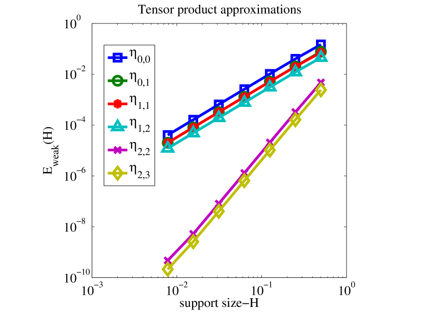
Figure 4: Weak-$\ast$ convergence of radial and tensor product distributions.

Next, we compare the accuracy of our approximations to a number of other delta distribution approximants that are commonly used in the literature (where these regularizations can be derived from discrete moment conditions (9) along with some other additional conditions being imposed). Specifically, we compare the regularizations constructed in Section 3.3.1 with four common regularizations obtained by solving discrete moment conditions (see [32], for example). In 2D, we construct all regularizations using tensor products. Following [32], we consider two hat functions with support $[-H,H]$ and $[-2H,2H]$ respectively:

$$\eta_{\text{hat},1}(r):=\begin{cases}1-\left|r\right|,&|r|<1,\\ 0,&\mbox{otherwise},\end{cases}\qquad\mbox{and}\qquad\eta_{\text{hat},2}(r):=\begin{cases}\frac{1}{4}\left(2-\left|r\right|\right),&|r|<2,\\ 0,&\mbox{otherwise}.\end{cases}$$ (43)

Both $\eta_{\text{hat},1}$ and $\eta_{\text{hat},2}$ are equivalent (modulo scaling) to the regularization $\eta_{1,1}(r)$ obtained in (32). Both of these hat functions satisfy the same number of compact $m$-moment conditions, but in practice $\eta_{\text{hat},2}$ is preferred since more quadrature points are present within its support [32].

We consider two additional regularizations defined in [32] based on the cosine function

$$\eta_{\cos}(z):=\frac{1}{4}\left(1+\cos(\pi z/2)\right),$$ (44)

and piecewise cubic function

$$\eta_{\text{cubic}}(z):=\left\{\begin{aligned} &1-\frac{1}{2}\left|z\right|-\left|z\right|^{2}+\frac{1}{2}\left|z\right|^{3},\qquad&&\left|z\right|\leq 1,\\ &1-\frac{11}{6}\left|z\right|+\left|z\right|^{2}-\frac{1}{6}\left|z\right|^{3},\qquad&&1<\left|z\right|\leq 2,\end{aligned}\right.$$ (45)

both of which are supported on $[-2H,2H]$. It is easy to see that $\eta_{\cos}$ is equivalent to our first moment approximation $\eta_{1,\cos}$ obtained using the trigonometric basis (36). We expect this approximation to have second-order weak-$\ast$ convergence if all quadratures were exact. However, as discussed in [32], $\eta_{\cos}$ only has first-order convergence when used to approximate the delta distribution [32] on a uniform grid and using a trapezoidal rule discretization for the moment conditions.

Figure 5 compares the weak-$\ast$ convergence of our tensor product distributions with the other discrete approximations mentioned above. It is clear that $\eta_{L1}$, $\eta_{L2}$ and $\eta_{\cos}$ all have second order convergence as expected. The only nontrivial case is $\eta_{\text{cubic}}$, which is not directly related to any of our previous approximations. It is interesting that even though this approximation is built to satisfy three discrete moment conditions [32], it appears to satisfy three continuous approximations as well.

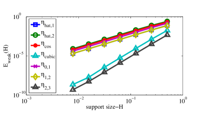
Figure 5: Comparing weak-$\ast$ convergence of the discrete approximations in [32] against our continuous tensor product distributions.

4 Applications to prototypical PDEs with approximate point sources

So far, we have been concerned with constructing approximate distributions that converge to the delta distribution in two specific modes. We now turn our attention to the error inherited by the solutions of a PDE where point sources are replaced by approximations $\tilde{\delta}_{H}$. That is, we wish to examine the error $\|u-u_{H}\|_{X}$ in some norm $X$, where $u$ and $u_{H}$ refer to solutions of (1) and $H$ denotes the support of $\delta_{H}$.

In practice, a PDE discretization with mesh size $h$ is used to approximate solutions to $\mathcal{L}u_{H}=\delta_{H}$. Suppose we fix $H>0$, then $\lim_{h\rightarrow 0}u_{H,h}=u_{H}$ provided we have chosen a convergent numerical method. If $\tilde{\delta}_{H}$ we choose is regular enough, then $u_{H}$ may itself be smooth enough for pointwise comparisons to be meaningful. The limit must be taken in an appropriate norm; however in practice we simultaneously vary $H$ and $h$, and must therefore be able to directly compare $u_{H,h}$ with $u$. The solution $u$ of $\mathcal{L}u=\delta$ may possess singularities. For example, if $\mathcal{L}$ is the Laplace operator with Dirichlet conditions on a disk, then $u$ is the Green’s function on the disk. Because this $u$ has a logarithmic singularity, we cannot compare $u_{H,h}$ to $u$ in a pointwise sense.

We must therefore address Question 4 raised in the Introduction: in what norm should we measure the convergence of $u_{H,h}\rightarrow u$? As might be expected, the answer depends on the PDE operator $\mathcal{L}$. One choice of norm $\|\cdot\|_{H}$ comes from taking $\|u-u_{H,h}\|_{\mathcal{H}_{0}^{s}(\Omega)}$, where the value of $s$ depends on $\mathcal{L}$ and must be sufficiently large so that $\delta\in\mathcal{H}^{-s}(\Omega)$. This choice is equivalent to comparing the Fourier coefficients of the two approximations. We use this approach to study scalar hyperbolic problems in Sections 4.3.1 and 4.3.2, and it is particularly instructive in the KdV equation which we consider in Section 4.4.

Another choice of norm is based on comparing functions pointwise in $\Omega$ away from the support of $\tilde{\delta}_{H}$. In other words, we use

$$\|w\|_{BH}:=\|w(1-\chi_{B(0,H)})\|_{L^{\infty}(\Omega)},$$ (46)

where $\chi_{\Gamma}$ is a usual $C^{\infty}$ cut-off function that takes the value $1$ on $\Gamma$ and smoothly decays to zero away from $\Gamma$. We apply this norm in Section 4.2 when studying the Helmholtz equation. The disadvantage of this choice is that as $H$ changes, so does the definition of the norm. Another norm that is intermediate between $\|\cdot\|_{BH}$ and $\|\cdot\|_{\mathcal{H}_{0}^{s}(\Omega)}$ is the $W_{\alpha}$–norm from Definition (11). We can use any of these to replace the norm $\|\cdot\|_{X}$ in the expression (2).

For fixed $H>0$, the behaviour of the discretization error $\|u_{H}-u_{H,h}\|_{X}$ will depend on the choice of numerical method and on the grid parameter $h$. However, even if we pick an excellent numerical method, if the error due to the regularization $\|u-u_{H}\|_{X}$ is not properly controlled then $u_{H,h}$ will not be a good approximation to $u$. We present examples highlighting this point below.

4.1 Elliptic PDEs

In this subsection, we consider the case when $\mathcal{L}$ is a linear second-order elliptic operator with zero boundary conditions. We first consider the simple situation corresponding to a constant coefficient operator, and then generalize to the situation where the coefficients may vary.

Suppose first that we denote by $L$ a constant-coefficient elliptic operator. Then, for $H>0$, let $\tilde{\delta}_{H}$ denote a regularization that satisfies the compact $m$-moment conditions. We then consider the problems

$$Lu=\delta, \text{for }x\in\Omega,\qquad \text{with }u=0\quad\text{for }x\in\partial\Omega,$$ (47)

$$Lu_{H}=\tilde{\delta}_{H}, \text{for }x\in\Omega,\qquad \text{with }u_{H}=0\quad\text{for }x\in\partial\Omega.$$ (48)

Theorem 1.

Let $u$ and $u_{H}$ solve problems (47) and (48) respectively, and let $m$ be the number of compact $m$-moment conditions satisfied by $\tilde{\delta}_{H}$. For all $x\in\Omega\backslash B(0,H)$ we have

$$\left|u(x)-{u}_{H}(x)\right|\leq C_{m}H^{m+1},$$ (49)

and therefore $\|u-u_{H}\|_{BH}=C_{m}H^{m+1}$, where $C_{m}>0$ is a constant that depends on $\Omega$ and $m$ but not on $H$.

Proof.

The solution of (47) is $u\equiv\mathcal{G}$, the Green’s function of the elliptic operator $L$ in $\Omega$. Let $\delta_{H}$ be an approximation of $\delta$ that satisfies the compact $m$-moment condition. Then for $x\in\Omega\setminus B(0,H)$,

$$\left|u(x)-{u}_{H}(x)\right| =\left|\mathcal{G}(x)-\int_{\Omega}\delta_{H}(y)\mathcal{G}(x-y)dy\right| \leq\left|C(\mathcal{G},m)H^{m+1}\right|,$$ (50)

where the last inequality follows from the estimate in (8) and the fact that the Green’s function $\mathcal{G}$ is infinitely differentiable away from the origin (see Theorem 6.5 in [25]). Therefore, $\|u-u_{H}\|_{BH}=\|(u(x)-u_{H}(x))(1-\chi_{B(0,H)})\|_{L^{\infty}(\Omega)}\leq C(\mathcal{G},m)H^{m+1}$. ∎

We also examine the difference $u-u_{H}$ in a weighted Sobolev norm in $\mathbb{R}^{n}$ for $n=2,3$. Our starting point is the recent work of [1] and [11]. Specifically, we use the key result in Section 2.1 of [1]: given $F\in W_{-\alpha}^{*}(\Omega)$, the constant-coefficient second order elliptic PDE $Lw=F$ in $\Omega$ with zero Dirichlet data possesses a unique solution $w\in W_{\alpha}(\Omega)$ provided that $\alpha\in(\frac{n}{2}-1,1)$ (the result in [1] was actually proved for more general elliptic operators). Moreover, the solution $w$ satisfies

$$\left\|w\right\|_{W_{\alpha}}\leq C_{*}\left\|F\right\|_{(W_{-\alpha})^{*}}.$$ (51)

Here $C_{*}>0$ is a positive constant that depends on $\Omega$, the PDE coefficients and $\alpha$; as $\alpha\rightarrow\frac{n}{2}-1$, the constant $C_{*}$ blows up. The regularity and bounds can be improved under certain assumptions on the coefficients of $L$. Now suppose that $u\in W_{\alpha}$ solves the PDE when $F=\delta$, whereas $u_{H}$ solves the problem when $F=\tilde{\delta}_{H}$, a regularization that satisfies the compact $m$-moment condition with support size $H$. By linearity and the bound in (20), it is easy to see that

$$\left\|u-u_{H}\right\|_{W_{\alpha}}\leq C_{*}\left\|\delta-\tilde{\delta}_{H}\right\|_{(W_{-\alpha})^{*}}\leq\tilde{C}_{*}H^{\frac{1}{\beta}(\alpha+(\beta-1)(m+1))}.$$ (52)

We can use this result to interpret the rate of convergence of different numerical schemes for solving elliptic PDEs. We can also make an statement about convergence in the $L^{2}_{\alpha}$ spaces. Given the solution $u\in W_{\alpha}$ and the approximation $u_{H}$ as before, suppose that $H=h^{\beta}$ where $h$ is a discretization parameter for the PDE, and assume that $\|u-u_{H}\|_{L^{2}(\Omega)\setminus B(0,h)}$ is small. We then have from the weighted Poincaré inequality that

$$\left\|u-\tilde{u}\right\|_{L^{2}_{\alpha}(B(0,h))}\leq C(\alpha)hH^{\frac{1}{\beta}(\alpha+(\beta-1)(m+1))}=C(\alpha)H^{\frac{1}{\beta}(\alpha+(\beta-1)(m+1)+1)}.$$ (53)

Consequently, in 2D and in the limit as $\alpha\to 0$ and $\beta\to 1$, we cannot obtain better than first-order convergence in $L^{2}(\Omega)$.

4.2 Numerical experiments with the Helmholtz equation

We now present numerical experiments that support our estimates of the regularization error in the case of elliptic PDEs with singular source terms. In particular, we solve the Helmholtz equation in one and two dimensions with homogeneous boundary conditions. Let $u$ and $u_{H}$ denote solutions of the problem

$$\Delta u+k_{0}^{2}u=F\quad\text{in }B(0,1)\qquad\text{and }u=0\quad\text{on }\partial\Omega,$$ (54)

with $F=\delta$ and $F=\delta_{H}$ respectively. Then set the wavenumber $k_{0}=10$ and consider solutions of (54) on the unit ball $B(0,1)$ in dimensions $n=1,2$. Our goal is to study the convergence of $u_{H}$ to $u$ using different measures of the error as $H\to 0$.

The solution $u_{H}$ of the regularized PDE does not have a closed form expression, and so we consider a numerical approximation $u_{H,h}$. In the following we use ChebFun [14] to solve for $u_{H,h}$ on a fine collocation grid, so that numerical errors $\|u_{h}-u_{H,h}\|$ are negligible compared to the approximation error $\|u-u_{H}\|$. For an elliptic problem like the Helmholtz equation, we expect high regularity away from the source. Therefore, a good choice of norm to compare $u$ and $u_{H,h}$ is $\|\cdot\|_{BH}$ as defined in (46). Because we want to vary both $H$ and $h$, we make a specific choice of norm

$$E_{\text{pointwise}}(H):=\|u-u_{H,h}\|_{B\bar{H}}=\left\|(u-u_{H,h})(1-\chi_{B(0,\bar{H})})\right\|_{L^{\infty}(B(0,1))},$$ (55)

where $\chi_{B(0,\bar{H})}$ is the standard $C^{\infty}$-cutoff function for the ball centered at the origin with radius $\bar{H}$ given by the largest support size of $\delta_{H}$ in our experiments. As a result, when $H\rightarrow 0$ we are always comparing $u$ and $u_{H,h}$ pointwise over the same set. We also define the quantity

$$R_{\text{pointwise}}(H):=\log_{2}\left(\frac{E_{\text{pointwise}}(H)}{E_{\text{pointwise}}(H/2)}\right),$$ (56)

which will be used with multiple values of $H$ to measure the rate of convergence of numerical solutions. In particular, as $H\to 0$ the value of $R_{\text{pointwise}}(H)$ should saturate to the expected rate of convergence from our analysis.

4.2.1 Helmholtz in $\mathbb{R}^{1}$: Pointwise convergence in a deleted neighborhood

We begin by considering the Helmholtz equation (54) in 1D, with $\Omega=B(0,1)\equiv[-1,1]$. The fundamental solution in this case is

$$u(x)=-\frac{\sin\left(\frac{k_{0}}{2}(1+\min\left\{x,0\right\})\right)\sin\left(\frac{k_{0}}{2}\left(1-\max\left\{x,0\right\}\right)\right)}{k_{0}\sin(k_{0})},$$ (57)

and belongs to $\mathcal{H}_{0}^{1}([-1,1])$. We take several values of the support size $H=1/2^{m}$ for $m=2,3,4,5$ and take the cut-off radius $\bar{H}=1/4$. Computed results for continuous delta approximations $\eta_{\text{cos}}$ and $\eta_{\text{cubic}}$ in the 1D Legendre basis are presented in Figure 6. In order to study the asymptotic rate of convergence of our approximations we report values of $R_{\text{pointwise}}(H)$ in Table 2 for different support sizes, and these results indicate that the ratios saturate to the expected rates of pointwise convergence of (49).

$R_{\text{pointwise}}(H)$					expected rate
support size ($H$)	$1/4$	$1/8$	$1/16$	$1/32$
$\eta_{0,1}$	1.7770	1.9438	1.9859	1.9965	2
$\eta_{1,2}$	1.4589	1.8761	1.9696	1.9924	2
$\eta_{2,3}$	3.7442	3.9371	3.9843	3.9961	4
$\eta_{\text{cos}}$	1.3331	1.8249	1.9558	1.9889	2
$\eta_{\text{cubic}}$	3.3330	3.8319	3.9579	3.9895	N/A

Table 2: Convergence rates for the 1D Helmholtz solution using the measure $E_{\text{pointwise}}(H)$ as defined in (55) for pointwise solution error away from the support of the delta distribution. The expected rates of convergence are obtained as in (49) and depend on the number of moment conditions that are satisfied by the approximation.

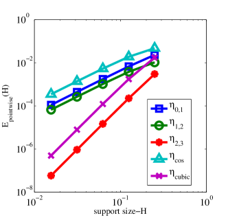
Figure 6: Pointwise error in the 1D Helmholtz solution, with three continuous polynomial approximations of the delta distribution (see Table 1) compared to two approximations (44) and (45).

Although these results demonstrate that $\eta_{\text{cubic}}$ and $\eta_{2,3}$ both exhibit fourth-order convergence, Figure 6 shows that the solution using $\eta_{2,3}$ is almost an order of magnitude more accurate for any given value of the support size $H$. This hints at a trade-off between choosing a more regular solution that is easier to compute numerically but is less accurate, and an approximation that is more difficult to resolve but gives a more accurate solution.

4.2.2 Helmholtz in $\mathbb{R}^{2}$: Pointwise convergence in a deleted neighborhood

We next consider the Helmholtz equation (54) on the unit disk in 2D, with the main purpose of this example being to test the radially symmetric delta approximations in Table 1. The Green’s function for the Helmholtz equation on the unit disk can be written in terms of Bessel functions as [15]

$$u(r,\theta)=-\frac{1}{4}Y_{0}(k_{0}r)+\frac{1}{4}\sum_{n=-\infty}^{\infty}\frac{J_{n}(0)Y_{n}(k_{0})}{J_{n}(k_{0})}J_{n}(k_{0}r)e^{in\theta}.$$ (58)

Because the radial delta approximations are symmetric, the solution $u_{H}$ is also clearly symmetric.

We then perform a numerical convergence study with parameters identical to those used in the previous one-dimensional Helmholtz example. Plots of the pointwise error are presented in Figure 7 and the corresponding ratios of successive errors $R_{\text{pointwise}}(H)$ are listed in Table 3. We see once again that the numerical rates of convergence are in agreement with the estimates from (49).

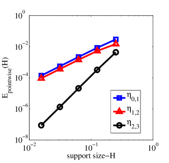
Figure 7: Convergence rates for the 2D Helmholtz solution using the error measure (55) and several radially-symmetric delta approximations.

$R_{\text{pointwise}}(H)$					expected rate
support size ($H$)	$1/4$	$1/8$	$1/16$	$1/32$
$\eta_{0,1}$	1.8010	1.9498	1.9874	1.9968	2
$\eta_{1,2}$	1.4964	1.8840	1.9715	1.9930	2
$\eta_{2,3}$	3.7560	3.9401	3.9822	3.9127	4

Table 3: Convergence rates for the Helmholtz solution in 2D, compared to the expected analytic rates of convergence in (49).

4.2.3 Helmholtz in $\mathbb{R}^{2}$: Convergence in $\|\cdot\|_{W_{\alpha}(B(0,1))}$

In this subsection we study the rate of convergence of numerical solutions to the 2D Helmholtz equation in the weighted Sobolev norms of Section 2.2. We consider a unit disk as above and study the same radial regularizations of the delta distribution. The main difference is that now the error is measured in the $W_{\alpha}(B(0,1))$ norm using

$$E_{W}(H):=\left\|u-u_{H,h}\right\|_{W_{\alpha}}:=\int_{B(0,1)}\left|\nabla u-\nabla u_{H,h}\right|^{2}\left|x\right|^{2\alpha}dx.$$ (59)

For our numerical simulations, we consider three different values of $\alpha=\{0.25,0.5,0.9\}$ to investigate the estimate in (52) and also take support of size $H=1/2^{n}$ for $n=\{2,3,\dots,8\}$. Figure 8 depicts convergence plots for various radial approximations (see Table 1) to the delta distribution and for different values of $\alpha$. We also list the error ratios $R_{W}(H)$ computing using (59) and (56), and report the corresponding results in Table 4. Note that in the limit as $h\to 0$, the rates saturate toward the estimate derived in (20) as $\beta$ approaches 1. The reason why we observe this mode of convergence is that $\beta>1$ corresponds to the case where the support of the associated $\delta_{H}$ goes to zero faster than the resolution of the numerical method. If we assume that this resolution is of the same order as the mesh size, then $\beta>1$ means that the support becomes smaller than the mesh size; but this is precisely the case when our quadrature schemes fail since there will not be sufficient quadrature points to integrate the function accurately. In our numerical experiments, we can study the limit of $h\to 0$ while the mesh is small enough so that the quadrature is still sufficiently accurate.

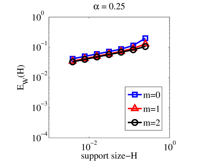
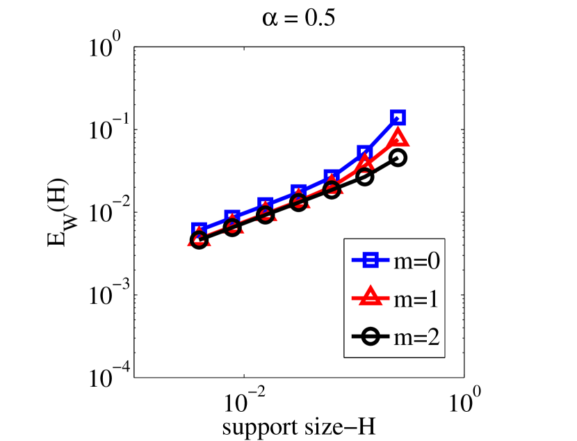
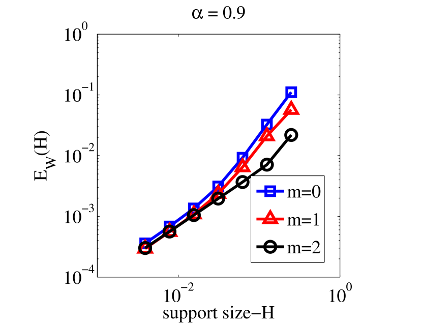
Figure 8: Error in the 2D Helmholtz solution using the $E_{W}(H)$ error measure from (59) based on the weighted Sobolev norms $W_{\alpha}$ for several values of $\alpha$.

$R_{W}(H)$								expected rate
support size ($H$)		$1/4$	$1/8$	$1/16$	$1/32$	$1/64$	$1/128$	for $\beta=1$
$\alpha=0.25$	$\eta_{0,1}$	0.8020	0.3946	0.2777	0.2613	0.2615	0.2656	$0.25$
	$\eta_{1,2}$	0.4834	0.3309	0.2695	0.2625	0.2654	0.2719
	$\eta_{2,3}$	0.3540	0.2684	0.2611	0.2624	0.2670	0.2746
$\alpha=0.5$	$\eta_{0,1}$	1.4268	0.9757	0.6074	0.5178	0.5035	0.5018	$0.5$
	$\eta_{1,2}$	1.0581	0.8471	0.5775	0.5130	0.5031	0.5025
	$\eta_{2,3}$	0.7701	0.5264	0.5061	0.5020	0.5015	0.5024
$\alpha=0.9$	$\eta_{0,1}$	1.7643	1.8157	1.5731	1.2033	0.9878	0.9207	$0.9$
	$\eta_{1,2}$	1.4424	1.6975	1.4557	1.1223	0.9599	0.9138
	$\eta_{2,3}$	1.6225	0.9483	0.9073	0.9018	0.9004	0.9001

Table 4: Rate of convergence of the 2D Helmholtz solution in the weighted Sobolev norm of $W_{\alpha}$ for different number of moments and different values of $\alpha$. The rates are compared to the expected rate of convergence from (52) when $\beta\to 1$. This shows that the rates are independent of the number of moments conditions in the limit as support size approaches the resolution of the numerical scheme.

4.3 Hyperbolic problems and the wave equation

In the previous section we applied regularized point sources to the solution of elliptic PDEs, and found that the solution exhibits pointwise convergence as long as we are sufficiently far away from the source. Also, the numerical solution converges weakly to the fundamental solution. In the following, we perform the analogous simulations for hyperbolic PDEs and see that these statements do not necessarily hold.

4.3.1 First-order wave equation in 1D

Consider the first-order wave equation on a periodic domain with an approximate impulse initial condition:

$$\left\{\begin{aligned} &u_{H,t}+u_{H,x}=0&&\text{ in }\mathbb{T}(0,2\pi)\times(0,T),\\ &u_{H}(x,0)=\delta_{H}(x)&&\text{ on }\mathbb{T}(0,2\pi)\times\{t=0\}.\end{aligned}\right.$$ (60)

The analytic solution $u_{H}(x,t)$ to this problem is a simple translation of the initial condition: $u_{H}(x,t)=\delta_{H}(x-t)$. If $u(x,t)$ denotes the solution of (60) with initial condition $\delta$, then $u(x,t)$ is a delta distribution supported at $(x-t)$. This means that the difference $|u-u_{H}|$ is exactly the regularization error $|\delta-\delta_{H}|$ and so we can only study convergence of the solution in the weak-$\ast$ sense. However, if we solve (60) numerically, then we can study the pointwise error $|u_{H,h}(x,T)-u_{H}(x,T)|$ for large $t$. Note that $u_{H}(x,t)=0$ outside the support of $\delta_{H}(x-t)$, but as we shall see shortly this is not true for long-time discrete solutions $u_{H,h}(x,T)$ owing to numerical dispersion.

To compute $u_{H,h}(x,t)$, we use a Fourier spectral collocation method in space with a leap-frog scheme in time, and implement a code based on Program 6 of [33]. In our simulations we use a uniform spatial grid of 1000 nodes to ensure that the initial condition $\delta_{H}(x)$ is captured accurately by the method. Time increments of size $\Delta t=\frac{1}{8}\Delta x$ are used to ensure that the CFL condition is satisfied.

We report the pointwise error at times $t=0$ and $t=36\pi$ (after 13 periods) and since $u_{H,h}(x,0)=\delta_{H}(x)=u_{H}(x,36\pi)$ on the grid, the pointwise error becomes

$$E(x)=\left|u_{H}(x,36\pi)-u_{H,h}(x,36\pi)\right|=\left|u_{H,h}(x,0)-u_{H,h}(x,36\pi)\right|.$$ (61)

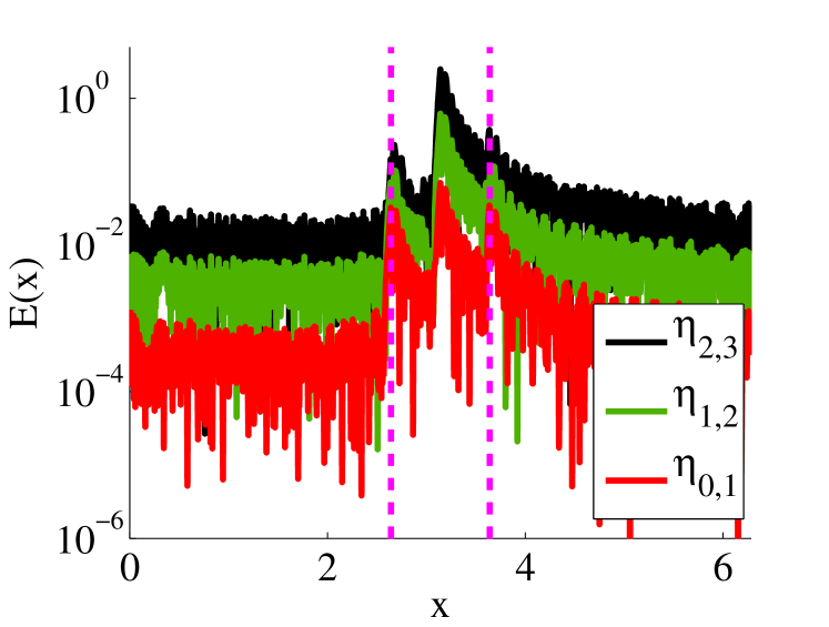
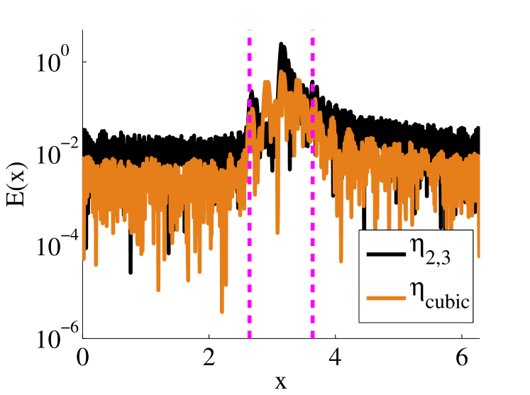
Figure 9: Pointwise error of solutions to the first order wave equation (60) after 13 periods. Dashed lines indicate the support of the $\delta_{H}$ approximations.

The results are displayed in Figure 9, from which we see that the error is larger for higher moment approximations both inside and outside the support of the regularized distributions. This demonstrates that the the error arises purely from the discretization of the PDE and not from the regularization, since $u_{H}(x,t)=\delta_{H}(x-t)$ is zero outside the interval $|x-t|\leq H$. More importantly, $u_{H,h}(x,t)$ does not converge to the true solution $u(x,t)$ outside the support of $\delta_{H}$.

Further insight into the cause of this growing numerical error is afforded by viewing the results from Figure 9 in the Fourier domain. Figures 10 compare the discrete Fourier transform of the initial and final solutions for various approximate delta distributions. Keeping in mind that the Fourier coefficients of the Dirac delta distribution are identically equal to 1, the quality of an approximation $\delta_{H}$ to the delta distribution can be measured by looking for Fourier modes that decay as slowly as possible with increasing wavenumber. However, we note that it is precisely the higher frequency modes that result in large (accumulating) discretization errors.

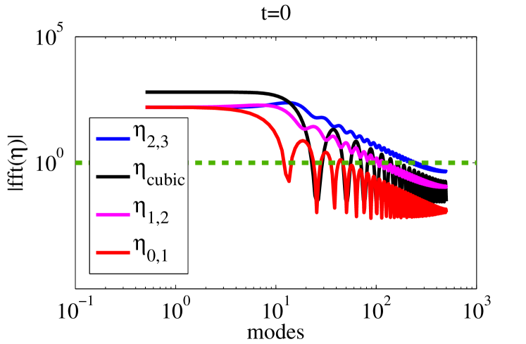
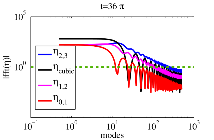
Figure 10: Comparison of the Fourier transform of the solution to the first order wave equation (60) at $t=0$ and $t=36\pi$. The green dashed line indicates the exact Fourier transform of the delta distribution.

This simple example identifies a number of issues that arise in the numerical solution of hyperbolic problems with singular delta sources when approximations to the delta distribution are used. In essence, the numerical solutions are dominated by dispersive errors that grow as the simulation time $T$ increases.

4.3.2 Second-order wave equation

Let $u(x,t)$ be the solution to the free-space 1-D wave equation $u_{tt}=u_{xx}$ with initial condition $u(x,0)=\delta(x)$ and zero initial velocity. Suppose that $u_{H}$ solves the same problem but with initial condition $u_{H}(x,0)=\tilde{\delta}_{H}(x)$, where $\tilde{\delta}_{H}$ has support $H$ and satisfies the compact $m$-moment condition. For fixed $x$, $u_{H}=0$ for $t\leq\left|x\right|-H$, and $u_{H}(x,t)$ has a transient behavior for $\left|x\right|-H\leq t\leq\left|x\right|+H$. But for $t\geq\left|x\right|+H$, $u_{H}$ will converge to the fundamental solution $u$ with $\mathcal{O}(H^{m+1})$ where $m$ is the number of moment conditions satisfied by $\tilde{\delta}_{H}$. This becomes clear by noting that for fixed $x$, $B(0,H)\subseteq B(x,t)$ for $t\geq\left|x\right|+H$ and so

$$\int_{B(x,t)}\delta_{H}(y)(t^{2}-\left|y-x\right|^{2})^{-1/2}dy=(t^{2}-\left|x\right|^{2})^{-1/2}+\mathcal{O}(H^{m+1}).$$

We expect, therefore, that $u_{H}$ will be close to the free-space fundamental solution, at least away from the support of $\delta_{H}$. In fact, $u_{H}(x,t)$ converges pointwise to the free-space fundamental solution $u(x,t)$ away from the wave front, regardless of the symmetry of the approximation $\delta_{H}$. We expect to see the lack of symmetry only within the wave front and not away from it.

While this result holds for the analytic solution $u_{H}(x,t)$, when computing a numerical solution $u_{H,h}(x,t)$ dispersive errors lead to qualitative differences. To illustrate this effect, we consider the wave equation on the unit square with homogeneous Dirichlet boundary conditions over the time interval $t\in[0,0.7]$:

$$\begin{cases}u_{tt}=u_{xx},&\text{in }[-1.1]^{2}\times(0,0.7],\\ u(x,0)=\delta_{H},&u_{x}(x,0)=u(-1,t)=u(1,t)=0.\end{cases}$$ (62)

For short times, we expect solutions to be the same as for the free-space wave equation, and in particular we expect them to be radially symmetric.

We use the radially symmetric discontinuous approximation $\delta_{H}(r)=\frac{1}{H^{2}}\eta_{2,2}(r/H)$ and the discontinuous tensor product approximation $\delta_{H}(x,y)=\frac{1}{H^{2}}\eta_{2,2}(x/H)\eta_{2,2}(y/H)$. Both regularizations satisfy two moment conditions, and we take $H=1/4$. As we shall see, the discontinuity at the endpoints amplifies the effect of dispersive errors and so this problem can be viewed as a worst case scenario.

We use two numerical methods to demonstrate the interplay between numerical dispersion and lack of symmetry for the tensor-product $\tilde{\delta}_{H}$. In the left column of Figure 11, we present the numerical solution using a spectral collocation method with Chebyshev basis functions and a fourth order Runge-Kutta time-stepping scheme. This code is available as program 20 of [33], and we choose $128^{2}$ collocation points. In the right column of Figure 11, we applied a finite element method on a uniform mesh with $128^{2}$ elements, using piecewise linear Lagrange elements for the spatial discretization and Crank-Nicolson time-stepping. The code in this case is available as step-23 in the tutorials for the deal.II software package [12]. We anticipate that dispersive numerical errors from this finite element scheme are larger than those in the spectral method.

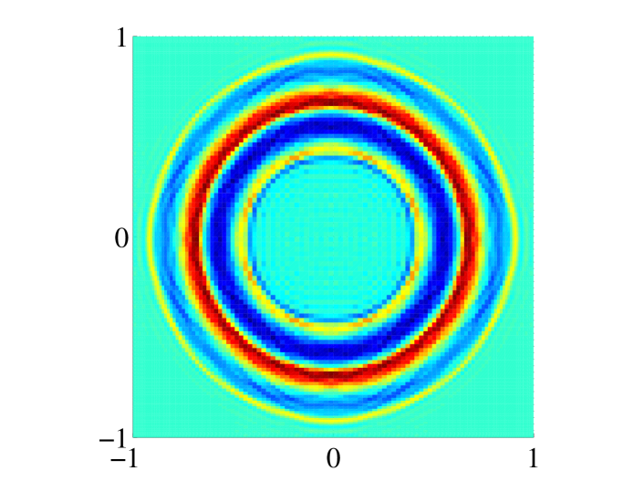
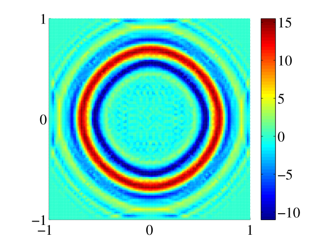
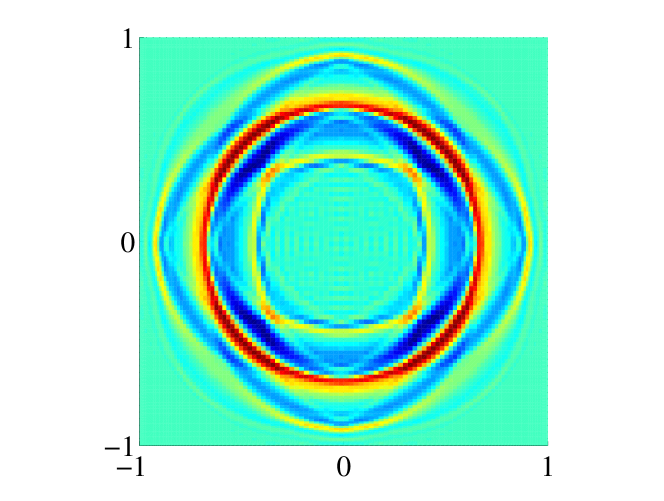
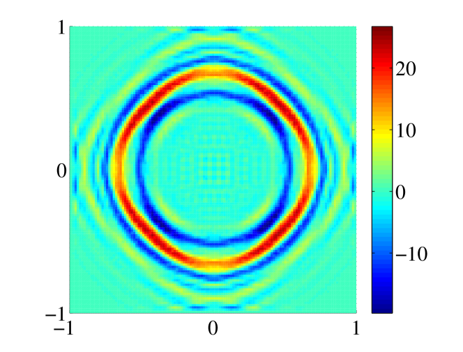
Figure 11: Numerical solution of the 2D wave equation using radially symmetric (top row) and tensor product (bottom row) approximations to the delta distribution. The left column contains the spectral collocation results and the right column those with the finite element method. Note the reflected waves that appear in the images on the right, that indicate waves moving faster than the original wave front and which are reflected by the boundary.

For both numerical methods, it is clear that the solution $u_{H,h}(x,t)$ for the tensor-product $\tilde{\delta}_{H}$ does not possess the expected radial symmetry of the exact solution. Furthermore, dispersive errors are more severe in case of the finite element solver, as expected; in particular, the finite element solution exhibits artificial waves moving faster than the original wave front. This issue is present for both radial and tensor-product $\tilde{\delta}_{H}$ approximations, but the fluctuations behind the wave front (closer to the origin) are significantly larger in case of the tensor product approximation for both spectral and finite element solvers.

Two points are illustrated here. First of all, a tensor-product approximation to the delta source term will yield numerical solutions that do not possess the symmetries of the exact solution, and this result is independent of the discretization method used. Secondly, the choice of numerical method is vital in terms of controlling dispersive errors.

4.4 Korteweg-de Vries (KdV) equation

In this final section we present numerical examples that illustrate issues that can arise when computing approximate solutions of nonlinear evolution PDEs with a regularized distribution as an initial condition. This is closely related to a common class of nonlinear problems with singular source terms. For example, in the immersed boundary framework the force from an elastic membrane enters the fluid momentum equations via a singular line source or chain of delta distributions [28]. We pick as a nonlinear test problem the KdV equation on the periodic domain $[-8\pi,8\pi]$:

$$u_{t}+6uu_{x}+u_{xxx}=0\quad\text{ in }\;\;\mathbb{T}([-8\pi,8\pi])\times(0,0.05]\quad\mbox{and}\;\;u(x,0)=\tilde{\delta}_{H}.$$ (63)

We have chosen a relatively large spatial domain and a short time interval in order to minimize boundary effects; sufficiently accurate numerical solutions of (63) in this setting will be good approximations of the free-space solution.

The free-space KdV equation with delta initial condition has no closed form solution. This problem has nonetheless been studied extensively and is known to consist of a single soliton moving to the right along with radiative waves propagating to the left (see [13]), with the soliton portion of the solution given by

$$u(x,t)\approx\frac{1}{2}\text{sech}^{2}\left(\frac{1}{2}(x-t)\right).$$ (64)

In numerical solutions of (63), we therefore expect to see a similar soliton combined with radiative waves, at least for short times.

To solve this problem numerically, we use the Fourier spectral solver implemented in Program 27 of [33] with $N=512$ Fourier modes, and a fourth-order Runge-Kutta time-stepping method. We observe that the solution is very sensitive to the smoothness of the $\delta_{H}$ approximation. Furthermore, controlling dispersive error is challenging, as is usually the case whenever simulating nonlinear wave equations.

As a first test, we aim to characterize the impact of support size for $\delta_{H}$ on the computed solutions. We perform our initial simulation using the delta approximation $\eta_{2,5}(r)$ from Section 3.3.1, which is a 5th order polynomial satisfying $m=2$ moment conditions and is differentiable everywhere (see Table 1). We construct $\delta_{H}$ from $\eta_{2,5}(r)$ as

$$\delta_{H}(x)=\frac{1}{H}\eta_{2,5}\left(\frac{|x|}{H}\right)\quad\text{where }x\in[-8\pi,8\pi],$$

and solve the KdV equation using our spectral scheme for $H=\pi,\pi/2,\pi/4$. At least in the limit as $H\rightarrow 0$, we expect $u_{H,h}$ to exhibit the expected soliton and radiative waves. Figure 12 depicts the numerical solutions $u_{H,h}(x,t)$ for several choices of $H$, with the left column showing solution in the $(x,t)$ plane, while the right column shows the time evolution of the Fourier modes. Note that the soliton portion of the solution (the light green strip in the middle of the plots) is captured well for all $H$. However, the lower order radiative waves differ considerably with $H$.

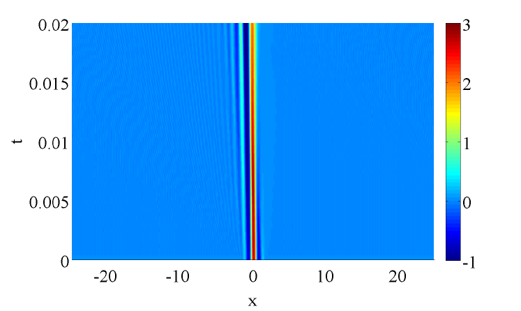
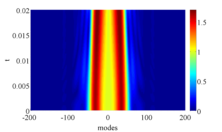
Figure 12: Solutions of the KdV equation with impulse initial condition using a smooth second moment approximation, $\eta_{2,5}$. Rows from top to bottom depict solutions for support of size $H=\pi$, $\frac{\pi}{2}$ and $\frac{\pi}{4}$. Images in the right column show the Fourier transform of the solution.

Next, we want to demonstrate the effect of different choices of moments on the computed solution. Since $\tilde{\delta}_{H}$ approximates $\delta$ with a rate depending on $m$, one may expect that the error $\|u-u_{H}\|_{X}$ should be improved with higher $m$. However, for the nonlinear wave equations, the error $\|u-u_{H,h}\|_{X}$ critically depends on the choice of the PDE discretization method; that is, the error is dominated by $\|u_{H}-u_{H,h}\|_{X}$. To demonstrate this, we study solutions of (63) with $\delta_{H}$ based on $\eta_{0,1}$, $\eta_{cubic}$ and $\eta_{2,5}$, and fix $H=\pi/4$ in each case. Recall that $\eta_{\text{cubic}}$ is a widely-used regularization that satisfies two discrete moment conditions [32]. The $\delta_{H}$ based on $\eta_{2,5}$ satisfies two continuous moment conditions, and is smooth. To provide a point of reference we also compute the solution to equation (63) with a Gaussian source term of the form

$$\delta_{\sigma}(x)=\frac{1}{\sqrt{2\pi\sigma^{2}}}\exp\left(\frac{-(x-1/2)^{2}}{\sigma^{2}}\right)$$ (65)

where we take $\sigma=1/64\pi$ and solve the problem on a very fine mesh of 8196 collocation points. The Gaussian source term is infinitely differentiable and so has optimal decay of Fourier modes.

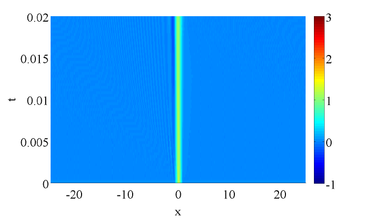
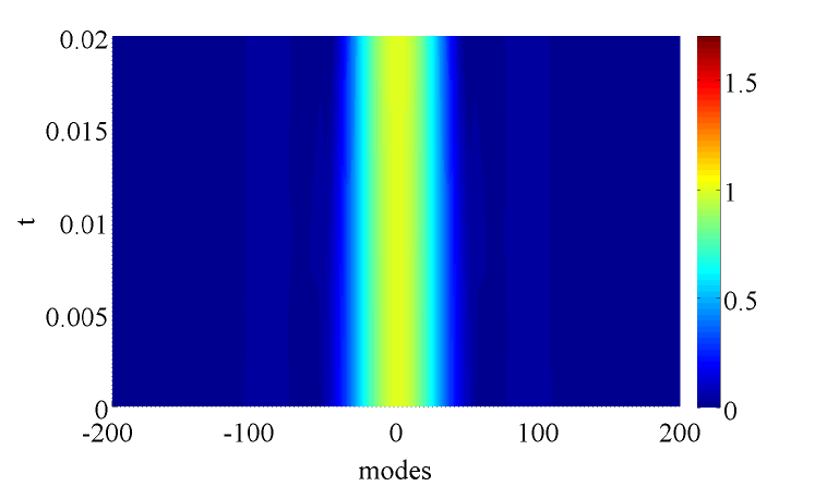
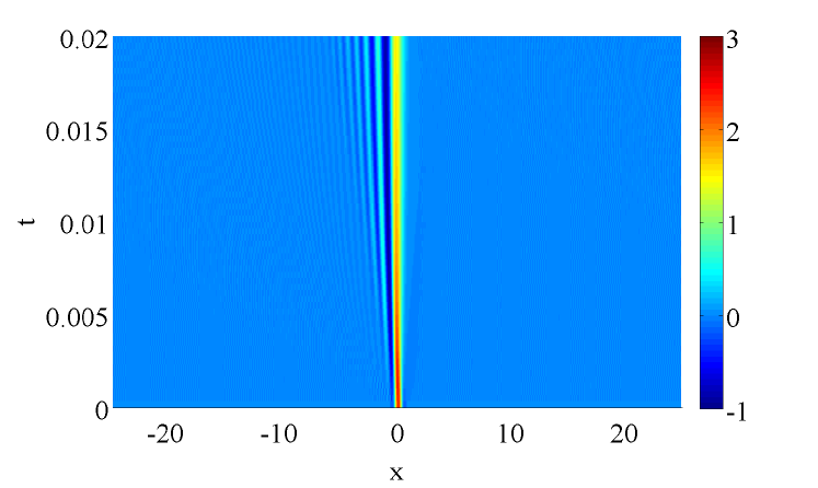
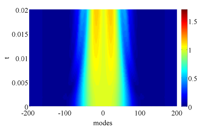
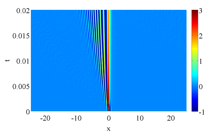
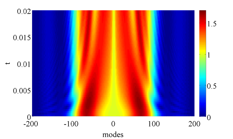
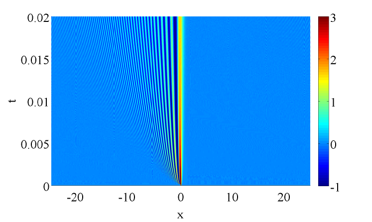
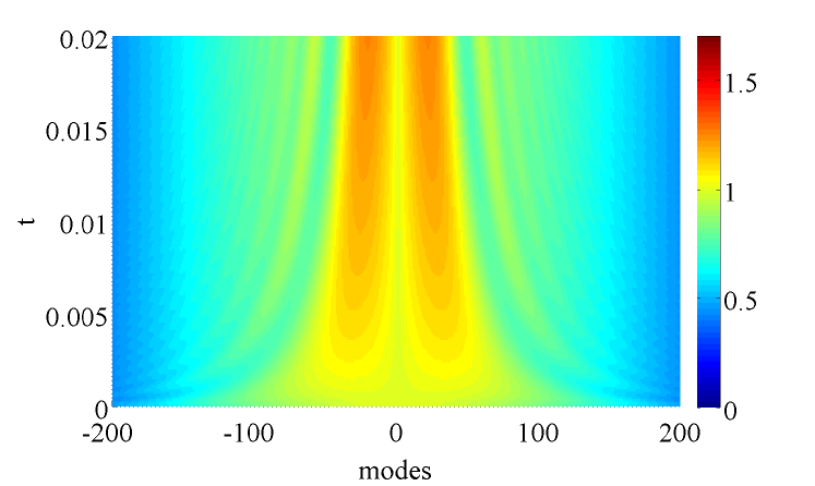
Figure 13: Solutions of the KdV equation with impulse initial condition using a first moment approximation, $\eta_{0,1}$ (top row), a discrete second moment approximation, $\eta_{cubic}$ (second row), a smooth second moment approximation $\eta_{2,5}$ (third row) and the reference solution using $\delta_{\sigma}$ on a very fine mesh (bottom row). The images in the right column are solutions in the Fourier domain.

Figure 13 depicts our solutions $u_{H,h}(x,t)$ for different choices of $\delta_{H}$ along with the reference solution with $\delta_{\sigma}$. The left column shows the computed solution in the $(x,t)$ plane. The right column shows the Fourier modes of the computed solution as time evolves. As in Figure 12, we see that the single soliton is captured for all choices of $\delta_{H}$. Furthermore, the numerical solutions using $\eta_{0,1}$ and $\eta_{\text{cubic}}$ are less noisy (and numerically better behaved) compared to $\eta_{2,5}$. However, the lower order radiative waves are very different in these approximations (compare to the reference solution in the bottom row). This example poses an interesting question. Recall that $\eta_{\text{cubic}}$ satisfies the same number of moment conditions as $\eta_{2,5}$ but the radiative waves look very different between the two. So if one is interested in capturing the radiative waves, it seems that $\eta_{2,5}$ is the better choice for fixed $H$. On the other hand, $\eta_{2,5}$ clearly has larger Fourier modes and so is more difficult to handle numerically.

This example clearly demonstrates that the choice of $\tilde{\delta}_{H}$ must be made carefully. If one is constrained to using a specific algorithm for the discretization of a PDE, then the choice of $\tilde{\delta}_{H}$ must be made accordingly. However, if the goal is to accurately capture the solution of a PDE, then one may want to first select a $\tilde{\delta}_{H}$ to minimize the regularization error $\|u-u_{H}\|_{X}$, and then construct a numerical method that achieves a controlled discretization error for $\|u_{H}-u_{H,h}\|_{X}$.

5 Conclusions

We began this article in Section 1 by posing four questions concerning approximations of singular source terms in PDEs. We argued that answers to the last two questions are required before the first two can be answered; that is, we first need to consider different modes of convergence when approximate distributions $\mathcal{S}_{H}\to\mathcal{S}$ and the corresponding solutions $u_{H,h}\to u$ before it is possible to make statements about what it means to have good approximations. Our response to these questions can be summarized as follows:

1. What form of convergence should be used to examine $\mathcal{S}_{H}\rightarrow\mathcal{S}$?

We provide two alternative answers to this question. Convergence in the weak-$\ast$ topology yields a system of moment conditions that permit the construction of sequences of distributions with arbitrary regularity and rates of convergence. We also consider convergence in the weighted Sobolev norm $\|\cdot\|_{(W_{-\alpha})^{*}}$ that allows one to study the interplay between the resolution of a numerical scheme and the support of the regularized source terms, and their effect on the rate of convergence of the numerical scheme.

1. What form of convergence should be used to examine $u_{H,h}\rightarrow u$?

2. How does the choice of approximation $\mathcal{S}_{H}$ affect the the convergence of $u_{H,h}\rightarrow u$?

The response to these two questions is problem-dependent and is conditioned on the type of PDE being considered. We showed that for a general class of elliptic PDEs, as well as the first- and second-order hyperbolic wave equations, numerical solutions converge pointwise in some parts of the domain. That is, we obtain pointwise convergence away from the support of the source term in case of elliptic PDEs and away from the wave front in hyperbolic problems. The rate of convergence depends on the rate of convergence of $\mathcal{S}_{H}\to\mathcal{S}$ in the weak-$\ast$ topology. We also showed that for elliptic PDEs we can obtain convergence in the weighted Sobolev norms $\|\cdot\|_{W_{\alpha}}$, where the convergence rate again depends on that of the regularization in the $\|\cdot\|_{(W_{-\alpha})^{*}}$ norm. Consequently, convergence of distributions $\mathcal{S}_{H}\to\mathcal{S}$ controls convergence of the solution. Finally, we can return to

1. How do we construct ‘good’ approximations $\mathcal{S}_{H}$ to $\mathcal{S}$?

If one is interested in approximating singular sources in the sense of distributions only, then arbitrarily high rates of convergence can be achieved simply by satisfying higher moment conditions. We proposed a general framework for solution of finite dimensional moment problems. Our approach is very flexible and allows construction of approximations using different bases. Furthermore, the lack of uniqueness in the moment equations affords us the advantage of being able to impose additional constraints on our constructions, such as smoothness at certain points in the domain.

If the final goal is instead to approximate solutions of an elliptic PDE, then we can obtain higher rates of pointwise convergence sufficiently away from the source by satisfying more moment conditions. Over the entire domain, the problem behaves differently. Convergence in the weighted Sobolev norm depends on the problem resolution and the support of the regularizations. In the limit when the support of the regularizations is the same order as the mesh size of a numerical solver, the rate of convergence is independent of the number of moment conditions and so there is no difference between a simple 0-moment approximation and a 2-moment approximation.

Applying our results in the context of hyperbolic PDEs proved more challenging. We presented numerical evidence that numerical errors due to dispersion become important for long-time solutions, and for this reason we were unable to observe the expected regularization error. Furthermore, for linear hyperbolic problems pointwise convergence should be considered away from the wave front rather than at a distance away from the support of the initial condition.

We also demonstrated that the choice of regularization can have a significant impact on solutions of PDEs. We looked in particular at the second-order wave equation and compared the use of a radial delta with a tensor-product approximation, showing that the latter produces non-symmetric solutions. Tensor product approximations to singular sources are used commonly in practice, but one must be cautious and pay careful attention to the qualitative effect of this class of approximations on the numerical solutions, especially for nonlinear problems and cases when advective terms dominate.

References

- [1] J. P. Agnelli, E. M. Garau, and P. Morin. A posteriori error estimates for elliptic problems with Dirac measure terms in weighted spaces. ESAIM: Mathematical Modelling and Numerical Analysis, 48:1557–1581, 2014.
- [2] N. I. Aheizer and M. Krein. Some questions in the theory of moments. Translations of Mathematical Monographs, Vol. 2. American Mathematical Society, Providence, RI, 1962.
- [3] J. T. Beale and A. Majda. Vortex methods. II. Higher order accuracy in two and three dimensions. Mathematics of Computation, 39:29–52, 1982.
- [4] E. Benvenuti. A regularized XFEM framework for embedded cohesive interfaces. Computational Methods in Applied Mechanics and Engineering, 2008:4367–4378, 2008.
- [5] E. Benvenuti, G. Ventura, N. Ponara, and A. Tralli. Accuracy of three-dimensional analysis of regularized singularities. International Journal for Numerical Methods in Engineering, 101:29–53, 2014.
- [6] R. P. Beyer and R. J. LeVeque. Analysis of a one-dimensional model for the immersed boundary method. SIAM Journal on Numerical Analysis, 29(2):332–364, 1992.
- [7] D. Boffi and L. Gastaldi. A finite element approach for the immersed boundary method. Computers & Structures, 81(8-11):491–501, 2003.
- [8] D. Boffi and L. Gastaldi. Discrete models for fluid-structure interactions: The finite element immersed boundary method, July 20, 2014. arXiv:1407.5261v1 [math.NA].
- [9] H. Brezis. Functional Analysis, Sobolev Spaces and Partial Differential Equations. Springer, 2011.
- [10] R. Cortez and M. Minion. The blob projection method for immersed boundary problems. Journal of Computational Physics, 161(2):428–453, 2000.
- [11] C. D’Angelo. Finite element approximation of elliptic problems with Dirac measure terms in weighted spaces: Applications to one-and three-dimensional coupled problems. SIAM Journal on Numerical Analysis, 50(1):194–215, 2012.
- [12] deal.ii finite element package, version 8.0.0. http://www.dealii.org/8.0.0, July 2013.
- [13] P. G. Drazin and R. S. Johnson. Solitons: An Introduction, volume 2. Cambridge University Press, 1989.
- [14] T. A. Driscoll, N. Hale, L. N. Trefethen, and editors. Chebfun Guide. Pafnuty Publications, Oxford, 2014.
- [15] D. G. Duffy. Green’s Functions With Applications. CRC Press, 2010.
- [16] B. Engquist, A.-K. Tornberg, and R. Tsai. Discretization of Dirac delta functions in level set methods. Journal of Computational Physics, 207:28–51, 2005.
- [17] L. C. Evans. Partial Differential Equations, volume 19 of Graduate Studies in Mathematics. American Mathematical Society, second edition, 2010.
- [18] E. B. Fabes, C. E. Kenig, and R. P. Serapioni. The local regularity of solutions of degenerate elliptic equations. Communications in Partial Differential Equations, 7(1):77–116, 1982.
- [19] A. Friedman. Generalized Functions and Partial Differential Equations. Dover Publications, 2005.
- [20] I. M. Gel’fand and N. Y. Vilenkin. Generalized Functions. Vol. 4: Applications of Harmonic Analysis. Academic Press, New York, 1964.
- [21] J. Heinonen, T. Kilpeläinen, and O. Martio. Nonlinear Potential Theory for Degenerate Elliptic Equations. Oxford Science Publications, 1993.
- [22] S. I. Kabanikhin. Inverse and Ill-posed Problems: Theory and Applications, volume 55 of Inverse and Ill-Posed Problems Series. Walter De Gruyter, 2011.
- [23] Y. Liu and Y. Mori. Properties of discrete delta functions and local convergence of the immersed boundary method. SIAM Journal on Numerical Analysis, 50(6):2986–3015, 2012.
- [24] Y. Liu and Y. Mori. convergence of the immersed boundary method for stationary Stokes problems. SIAM Journal on Numerical Analysis, 52(1):496–514, 2014.
- [25] W. McLean. Strongly Elliptic Systems and Boundary Integral Equations. Cambridge University Press, 2000.
- [26] Y. Mori. Convergence proof of the velocity field for a Stokes flow immersed boundary method. Communications on Pure and Applied Mathematics, LXI:1213–1263, 2008.
- [27] S. J. Osher and R. P. Fedkiw. Level Set Methods and Dynamic Implicit Surfaces. Springer, 2003.
- [28] C. S. Peskin. The immersed boundary method. Acta Numerica, 11:479–517, 2002.
- [29] J.-P. Suarez, G. B. Jacobs, and W.-S. Don. A high-order Dirac-delta regularization with optimal scaling in the spectral solution of one-dimensional singular hyperbolic conservation laws. SIAM Journal on Scientific Computing, 36(4):A1831–A1849, 2014.
- [30] A.-K. Tornberg. Multi-dimensional quadrature of singular and discontinuous functions. BIT, 42(3):644–6695, 2002.
- [31] A.-K. Tornberg and B. Engquist. Regularization techniques for numerical approximation of PDEs with singularities. Journal of Scientific Computing, 19(1–3):527–552, 2003.
- [32] A.-K. Tornberg and B. Engquist. Numerical approximations of singular source terms in differential equations. Journal of Computational Physics, 200(2):462–488, 2004.
- [33] L. N. Trefethen. Spectral Methods in MATLAB. SIAM, Philadelphia, PA, 2000.
- [34] J. Waldén. On the approximation of singular source terms in differential equations. Numerical Methods for Partial Differential Equations, 15(4):503–520, 1999.
- [35] Y. Yang and C.-W. Shu. Discontinuous Galerkin method for hyperbolic equations involving -singularities: negative-order norm error estimates and applications. Numerische Mathematik, 124(4):753–781, 2013.
- [36] S. Zahedi and A.-K. Tornberg. Delta function approximations in level set methods by distance function extension. Journal of Computational Physics, 229:2199–2219, 2010.