Characterizing an Entangled-Photon Source with Classical Detectors and Measurements

Abstract

Quantum state tomography (QST) is a universal tool for the design and optimization of entangled-photon sources. It typically requires single-photon detectors and coincidence measurements. Recently, it was suggested that the information provided by the QST of photon pairs generated by spontaneous parametric down-conversion could be obtained by exploiting the stimulated version of this process, namely difference frequency generation. In this protocol, so-called “stimulated-emission tomography” (SET), a seed field is injected along with the pump pulse, and the resulting stimulated emission is measured. Since the intensity of the stimulated field can be several orders of magnitude larger than the intensity of the corresponding spontaneous emission, measurements can be made with simple classical detectors. Here, we experimentally demonstrate SET and compare it with QST. We show that one can accurately reconstruct the polarization density matrix, and predict the purity and concurrence of the polarization state of photon pairs without performing any single-photon measurements.

Quantum information is an important emerging technology nielsen_quantum_2000 , and entanglement is its essential ingredient. It plays a vital role in tasks such as quantum computation Raussendorf_measurement_2003 ; walther_experimental_2005 , quantum metrology boto_quantum_2000 ; mitchell_super-resolving_2004 , and quantum key distribution Ekert_quantum_1991 ; ursin_entanglement_2007 ; Jennewein_quantum_2000 , and so progress in the development of high-quality entanglement sources is of central importance for advances in quantum information technology.

For any source of entangled states to be useful, it must be characterized. The standard method for doing this is quantum state tomography (QST) james_measurement_2001 . In principle, QST provides a complete description of the quantum state, from which one can evaluate the suitability of a source for any proposed application. But it is well-known that QST is a resource-intensive task. The quality of the tomographic estimate depends on the amount of data that one is able to acquire gill_state_2000 ; Okamoto_experimental_2012 ; mahler_adaptive_2013 and analyse gross_quantum_2010 , with more data typically resulting in a higher-quality estimate.

In this work, we investigate a particular physical system – entangled-photon pairs generated via spontaneous parametric down-conversion (SPDC) in a pair of BBO crystals – and show how the corresponding stimulated process, namely difference frequency generation (DFG), can be used to reconstruct the polarization density matrix of the two-photon state that arises in the spontaneous process. The signal generated by DFG can be several orders of magnitude more intense than that observed in SPDC, making it possible to estimate the quantum states produced by such sources very rapidly and efficiently. Liscidini_Stimulated_2013 . This is particularly important en route to the development of “on-chip” sources of entangled states horn_Monolithic_2012 ; orieux_direct_2013 ; horn_inherent_2013 ; as in the case of integrated electronic circuits, such sources are typically produced in large numbers, and fast and efficient characterization procedures are required.  The approach of “stimulated emission tomography” (SET) we demonstrate here would also allow for the full quantum characterization of sources with very low photon-pair generation rates, for which characterization by conventional QST might not even be feasible.  While an experiment exploiting the relation between stimulated and spontaneous emission to measure spectral correlations between the spontaneously generated photons has been performed recently eckstein_direct_2013 ; Fang_fast_2014 , the full tomography of photon pairs using SET has yet to be demonstrated.  That is what we undertake here.

As test case for SET, we use our polarization-entangled photon source (an SPDC “sandwich source”Kwiat_typeII_1995 ) which is illustrated in Fig. 1a; here a pair of nonlinear birefringent crystals is mounted with their optic axes orthogonal.  In an idealized picture, when a diagonally polarized pump pulse is incident the first crystal could produce pairs of horizontally polarized photons in the signal and idler modes (taking $|V\rangle_{{p}}\rightarrow|HH\rangle_{s,i}$), or the second crystal could produce vertically polarized photon pairs (taking $|H\rangle_{{p}}\rightarrow|VV\rangle_{s,i}$). Thus, if the source  – i.e. the pump pulse, the nonlinear crystals, and the collection optics – is appropriately configured altepeter_Phase-compensated_2005 ; Rangarajan_optimizing_2009 , SPDC results in the generation of a polarization-entangled state $(|HH\rangle_{s,i}+|VV\rangle_{s,i})/\sqrt{2}$.

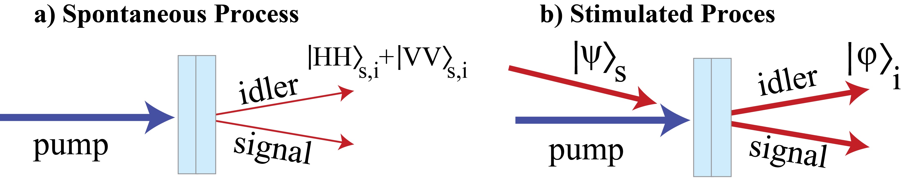
Figure 1: a) A simple cartoon of a SPDC “sandwich” source which produces entangled-photon pairs. b) A stimulated version of the SPDC sandwich source, now a seed beam is sent into the signal mode to stimulate light into the idler mode.

To characterize this state using QST, the polarization of each photon is measured in several different bases. Experimentally, this is typically done by sending each photon to a set of waveplates and a polarizer (Fig. 2b), and estimating the probability that both photons are transmitted. For example, if both polarizers are aligned in the horizontal direction we can estimate $\mathcal{P}_{H,H}$. For two-photons, 16 such probabilities are sufficient to constrain the two-photon polarization state. Thus, these measurements can be used to estimate the two-photon polarization density matrix james_measurement_2001 ; see the Supplement for more details.

In SET, a strong seed beam is constructed to mimic the signal photons of the pair that could be generated by spontaneous emission (Fig. 1b), including all possible polarizations. Consequently, in the presence of the seed beam, an idler beam is generated by DFG. Two of us predicted earlier Liscidini_Stimulated_2013 that the biphoton wavefunction characterising the pairs that would be emitted by SPDC acts as the response function relating the idler beam to the seed beam in DFG. Thus, by changing the polarization of a properly configured seed beam $|\psi\rangle_{s}$ and performing measurements on the polarization of the stimulated idler $|\phi\rangle_{i}$, conclusions can be drawn about the two-photon state that would be generated in the absence of the seed. For example, by using a horizontally polarized seed beam and measuring the stimulated beam in the horizontal basis, one can compute the probability of detecting a horizontally polarized signal photon and a horizontally polarized idler photon in a spontaneous experiment $\mathcal{P}_{H,H}$. In an ideal situation, this probability is simply $\mathcal{P}_{H,H}={I_{H}^{\mathrm{stim}}}/{I_{H}^{\mathrm{seed}}}$, where $I_{H}^{\mathrm{stim}}$ is the intensity of the horizontally polarized simulated light and $I_{H}^{\mathrm{seed}}$ the intensity of the seed light. This procedure can be repeated for other polarization combinations, yielding the same information as QST. Thus, SET obtains sufficient information to reconstruct the full two-photon polarization state.

The source and our implementation of QST and SET are shown in Fig. 2. Our sandwich crystals are a pair of $1$ mm - thick BBO crystals. To generate entangled photons, a “temporal compensation” crystal is placed before the sandwich crystals to pre-delay one component of the pump polarization so that, by the time the photon-pairs emerge from the sandwich crystals, the $|H,H\rangle_{s,i}$ pairs are temporally indistinguishable from the $|V,V\rangle_{s,i}$ pairs. Our source is pumped with $\approx 200$ fs-long pulses which are centred at $400$ nm, with an average power of $500$ mW. This pump light is generated by frequency-doubling $1.5$ W (average power) of $800$ nm light from a femtosecond Ti:Sapph laser with a 76 MHz repetition rate, using a $2$ mm-long BBO crystal. The $400$ nm pump pulse is focused into the crystal with a $15$ cm lens, resulting in a beam waist of $\approx 50$ $\mu$m in the crystal.

The collected signal and idler modes are defined by two single-mode fibres (with a numerical aperture of $0.12$), a $10$ cm focal-length lens to collimate the emission, and two $4$ mm aspherical lenses to focus the signal and idler beams into the fiber. Light is collected from a spot size that is about the same size as the focused pump, as prescribed by Ling et al. ling_absolute_2008 .  Finally, each mode is filtered with a $10$ nm spectral filter centred at $800$ nm. This produces approximately $15,000$ polarization-entangled photon pairs per second coupled in the signal and idler modes, with a coupling efficiency (pairs/singles) of $\approx 15\%$. These photons are then directed to a standard QST apparatus (see Fig. 2b), where the photon pairs are detected with single-photon detectors, and coincidence counts are registered with a homebuilt FPGA-based coincidence circuit. When the source is nominally configured to generate the maximally-entangled state $(|HH\rangle_{s,i}+|VV\rangle_{s,i})/\sqrt{2}$, QST yields the polarization density matrix shown in Fig. 3a, which has a fidelity of $\approx 0.951$ with the maximally entangled state.

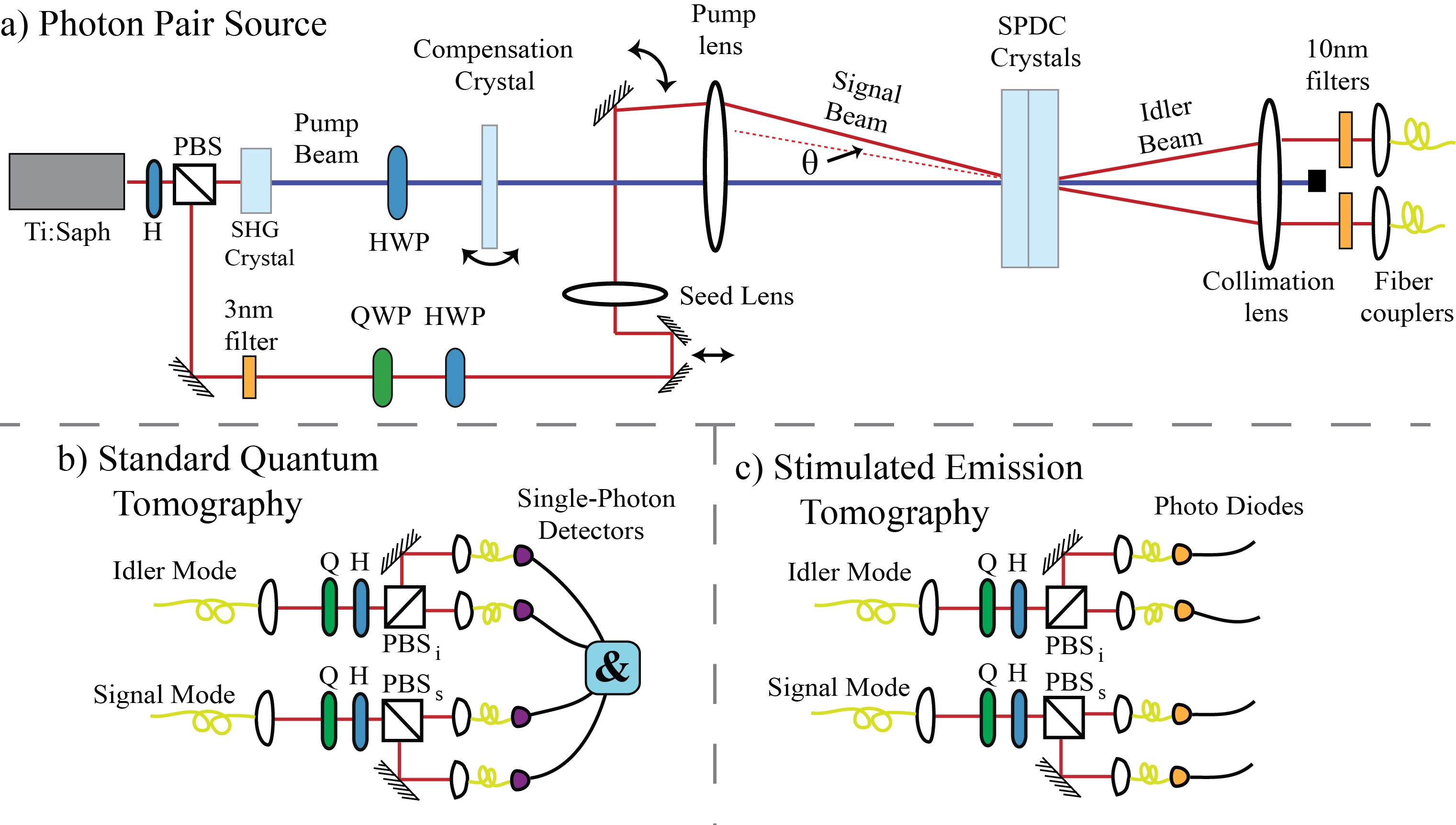
Figure 2: a) A sketch of our entangled-photon source and the generation of our seed beam for stimulated emission tomography. The signal and idler modes are coupled into a pair of single-mode fibres, and sent to a tomography apparatus which can be configured for either quantum or stimulated-emission tomography. b) The standard quantum tomography apparatus. It consists of a pair polarization measurements on each mode (implemented using waveplates and polarizing beamsplitter cubes). For quantum state tomography, the output modes of each cube are coupled to single-photon detectors and coincidences between the various detector pairs are monitored. c) The stimulated emission tomography apparatus. It is almost identical to quantum tomography, but now photo diodes replace the single-photon detectors and there is no need for any coincidence measurements. For both quantum and stimulated-emission tomography, both ports are monitored to aid in normalizing the data to correct for different detector efficiencies.

To perform SET, a seed field is constructed by diverting approximately $150$ mW of the original $800$ nm pulsed Ti:Sapph light; in this configuration, the $400$ nm average pump power is also $150$ mW. Note that this is not a strict application of SET as proposed earlier Liscidini_Stimulated_2013 , since it makes use of a pulsed earlier Liscidini_Stimulated_2013 , since it makes use of a pulsed seed and not a CW seed. This can introduce errors in the determination of the polarization density matrix when the biphoton wavefunction depends strongly on the photon energy within the seed pulse bandwidth. To compensate for this, we used a $3$ nm spectral filter to lengthen the seed pulse. Finally, since the pump and the seed pulse have different frequencies, they experience different spatial walk-offs. To minimize this effect the seed beam waist is made much larger than the pump beam waist (approximately $1000$ $\mu$m), so that good spatial overlap is maintained as both beams traverse the nonlinear crystals. Note that if the “seed lens” (Fig. 2a) is removed, then the seed pulse would have a waist of $50$ $\mu$m in the crystal; in this configuration the different spatial walk-offs become relevant. As we discuss in Section 3 of the Supplement, this can lead to polarization dependent losses, which can introduce errors in the SET reconstruction. When the $1000$ $\mu$m seed beam is temporally and spatially overlapped with the pump pulse in the SPDC crystals, we observe a stimulated idler output power of approximately $100$ $\mu$W coupled into the single-mode fibre. The polarization measurements for SET are then performed in the same apparatus used for QST, but with the single-photon detectors replaced by photo-diodes (Fig. 2c).

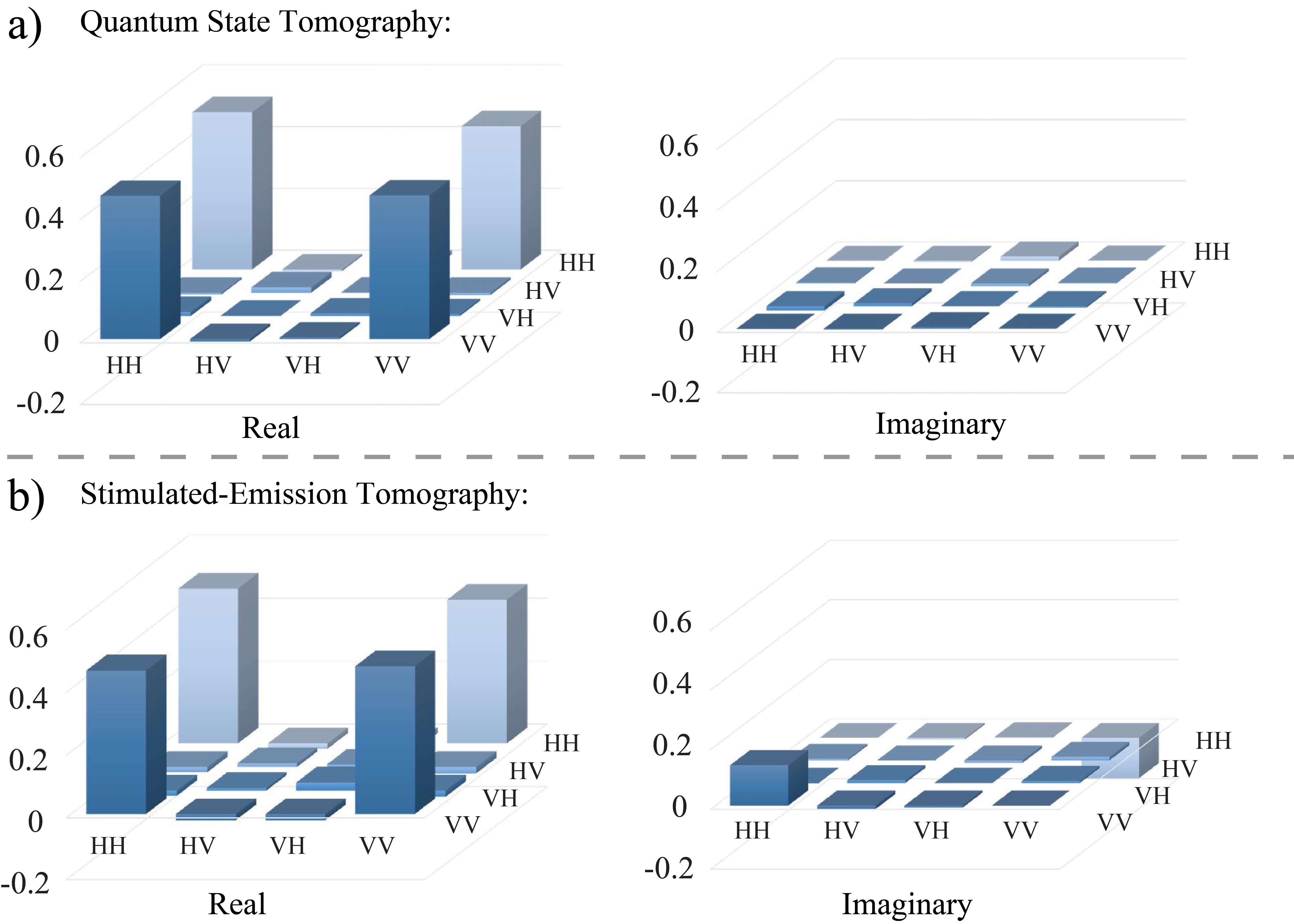
Figure 3: Two-photon density matrices reconstructed by (a) standard quantum state tomography and (b) stimulated emission tomography (SET). The SET reconstruction is based on the single-photon density matrices shown in Table 1 of the Supplement. The density matrices reconstructed using the two methods have a fidelity of 0.963 with each other.

We prepare the seed signal pulse in six different polarization states, and, for each seed configuration, we measure the intensity of the stimulated idler in the same six different polarization states (see Table 1 of the Supplement). These data are fed into our modified least-squares fitting algorithm (see Section 1 of the Supplement) to reconstruct the quantum state. When the source is nominally configured to generate the maximally entangled state $(|HH\rangle_{s,i}+|VV\rangle_{s,i})/\sqrt{2}$, SET yields the polarization density matrix shown in Fig. 3b, which has a fidelity of $\approx 0.939$ with the maximally-entangled state.

The results of QST and SET are close but significantly different; the quantum fidelity of one with respect to the other is $0.963$ jozsa_fidelity_1994 . The difference arises because the phase between $|HH\rangle_{s,i}$ and $|VV\rangle_{s,i}$ extracted by SET and QST disagree by $0.289$ rad; this is manifest in the larger imaginary components in the SET prediction. Were the phases artificially set to be identical, the fidelity between the two estimates would increase to $0.982$.

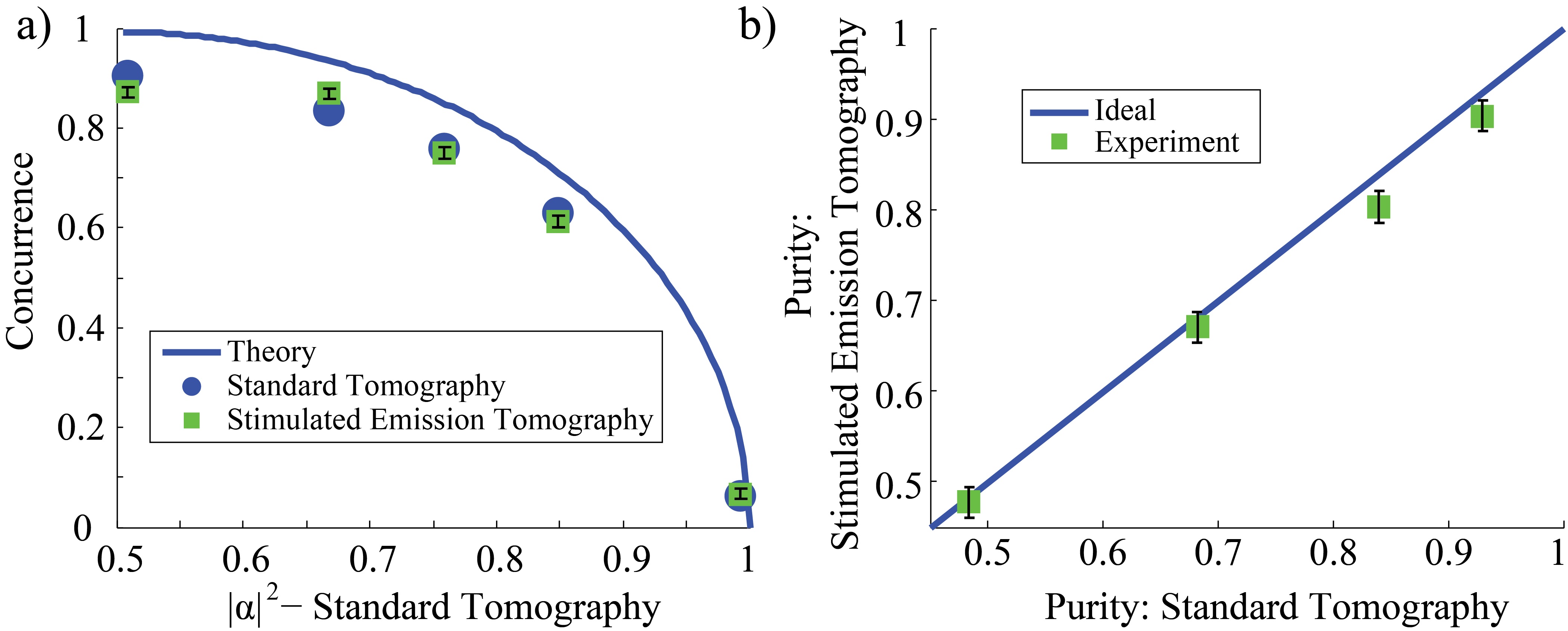
Figure 4: a) A plot of the concurrence versus $|\alpha|^{2}$; $|\alpha|^{2}$ was extracted from quantum state tomography (QST). These data were taken for entangled states of the nominal form: $\alpha|HH\rangle+\beta|VV\rangle$. The green squares were extracted from stimulated-emission tomography (SET), the blue circles from are the QST, and the blue curve is a simple theory calculation assuming perfectly pure states. b) A plot of the purity extracted from SET versus the purity extracted from standard QST. For these data $|\alpha|^{2}\approx 0.5$, and the compensation crystal in the source was systematically misaligned to reduce the purity.

We will return to the disagreement between QST and SET below, but first note that measures of entanglement (such as the concurrence) are not sensitive to the phase between $|HH\rangle_{s,i}$ and $|VV\rangle_{s,i}$. Hence, we should expect that QST and SET would predict essentially the same amount of entanglement.

To confirm this, in one set of experiments we prepare states of the form $\alpha|HH\rangle_{s,i}+\beta|VV\rangle_{s,i}$ and vary $|\alpha|$ from $1/\sqrt{2}$ to 0 (by rotating the pump polarization with a half waveplate). This gradually decreases the concurrence of the source (while keeping the state approximately pure). We perform both SET and QST on states in this range; the concurrences predicted by both techniques are plotted versus $|\alpha|^{2}$ in Fig. 4a. Since the concurrence is independent of the phase between $|HH\rangle_{s,i}$ and $|VV\rangle_{s,i}$, the QST and SET results agree extremely well.

The most common problem plaguing polarization-entanglement sources is a reduced coherence between $|HH\rangle_{s,i}$ and $|VV\rangle_{s,i}$, which results in a loss of entanglement Rangarajan_optimizing_2009 . Therefore, we performed a second set of experiments, showing that SET can characterize this loss. In sandwich sources pumped with an ultra-fast laser, such as ours, the entanglement is often reduced by imperfect temporal compensation; the $|HH\rangle_{s,i}$ and $|VV\rangle_{s,i}$ photons are emitted in distinguishable temporal modes, so that ignoring these temporal modes effectively decoheres the state. To see how QST and SET capture this loss of polarization entanglement, we initially set (using QST) our source to produce the nominal state $(|HH\rangle_{s,i}+|VV\rangle_{s,i})/\sqrt{2}$ with high purity, and then began to misalign the compensation crystal by rotating it in $10^{\circ}$ increments, finally removing it altogether, to reduce the purity of the states. Both QST and SET were performed on these states, and the purities yielded by the two techniques are in good agreement, as shown in Fig. 4b.  Again, this agreement is independent of the actual phase between $|HH\rangle_{s,i}$ and $|VV\rangle_{s,i}$.

We now return to the disagreement in the phase between QST and SET.  A deeper investigation allowed us to establish that the phase between $|HH\rangle_{s,i}$ and $|VV\rangle_{s,i}$ extracted by SET is a function of the incidence angle of the seed beam ($\theta$ in Fig. 2) as illustrated in Fig. 5. In particular, it varies by $\approx 0.312$ rad per mrad deviation of the seed beam (extracted from the fit shown as a dashed line). This is simply because the spontaneously generated photons can be emitted at different angles, and the nonlinear crystals are birefringent. The magnitude of our experimentally-measured angle-dependent phase agrees well with the theory of Altepeter et al. altepeter_Phase-compensated_2005 , which predicts $0.461$ rad per mrad for our crystals.

In our QST experiment, pairs are collected over a transverse momentum range $\Delta k_{f}=\lambda/(\pi\omega_{f})\approx$ $5$ mrad, which can be estimated by observing that the single-mode fibers collect from a spot size of $\omega_{f}\approx 50$ $\mu$m in the crystal; the angular phase-matching bandwidth of our SPDC crystals is $\approx 3.5$ mrad SNLO .  Thus, the polarization matrix determined by QST is itself the results of averaging over the emission angles, and the identification of a state (as in Fig. 3a) such as $(|HH\rangle_{s,i}+|VV\rangle_{s,i})/\sqrt{2}$ indeed is truly only nominal; in fact, there is entanglement between polarization degrees of freedom and emission angle.  This is a well-known result in bulk down-conversion experiments where one often collects pairs over broad range to increase the detection rate altepeter_Phase-compensated_2005 ; Rangarajan_optimizing_2009 .

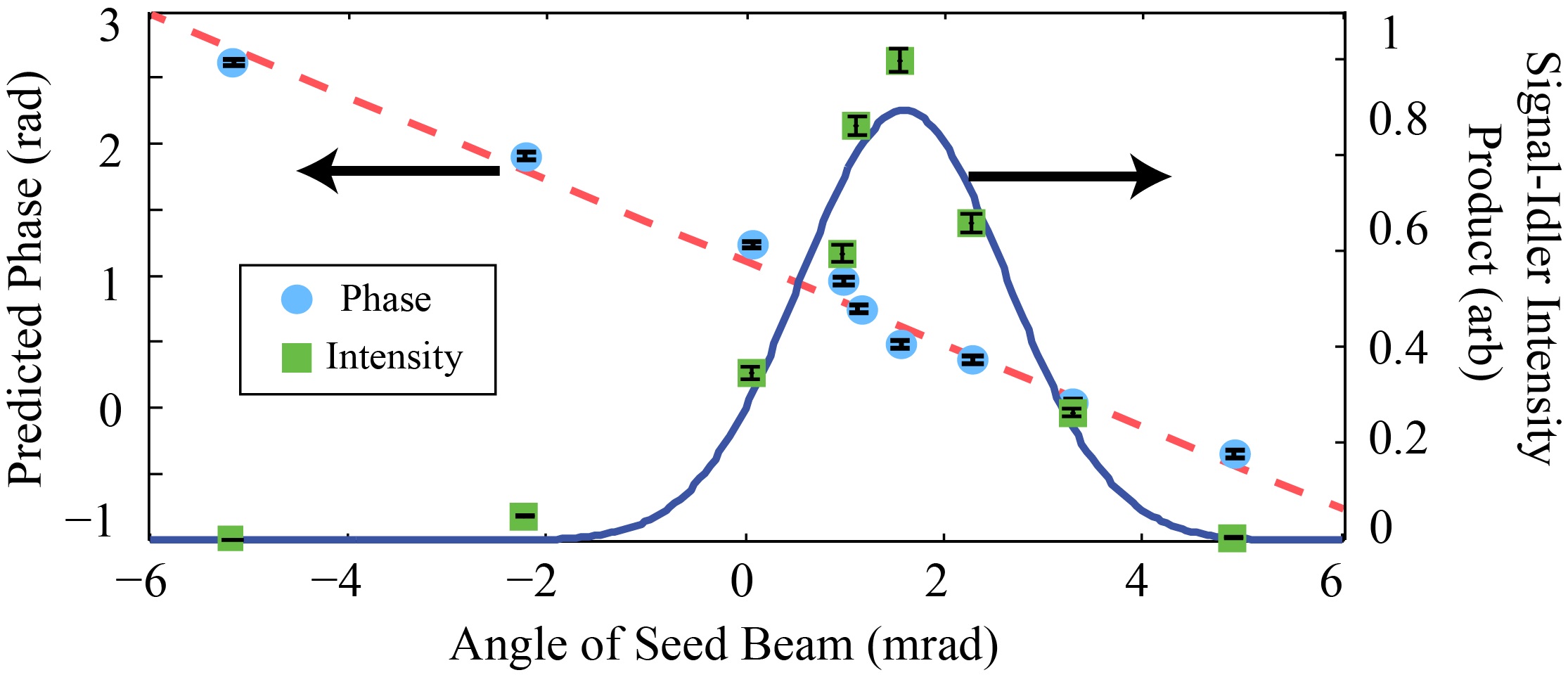
Figure 5: Effect of the seed angle. The circles are the phase of the entangled state predicted by SET plotted versus the seed incidence angle. The dashed line is a linear fit to these data, indicating that the phase changes by 0.312 rad per mrad. The squares are the product of the experimentally measured intensity of the signal and idler light that is coupled into single-mode fiber. The solid curve is a Gaussian fit to these data.

In contrast, in SET our seed pulse has a waist of $\omega_{s}\approx 1000$ $\mu$m, with a range in transverse momenta of only $\Delta k_{s}\approx 0.3$ mrad. Thus, one can selectively explore the density matrix of pairs generated at specific angles, so that SET can easily capture the effect of the phase dependence on the emission angle. Hence SET will allow us to investigate the biphoton wave function that would be generated by SPDC in even more detail than the usual, emission-angle averaged QST. In fact, the disagreement with QST (as in comparing Fig. 3a and Fig. 3b) can be understood as the ability of SET to look “deeper” into the biphoton wave function than standard QST, and actually study the entanglement between polarization and emission angle.  It should be possible to obtain the nominal QST matrix shown in Fig. 3a by using SET, scanning over the same angular ranges, and averaging the results.  We will return to these kinds of characterizations in a future publication; in fact, it has already been reported eckstein_direct_2013 ; Fang_fast_2014 that the extraction of frequency correlations of entangled photons that would be observed in a spontaneous experiment can be done with a much higher resolution in a stimulated experiment.

In conclusion, we have experimentally demonstrated that sources of entangled photons generated by SPDC can be characterized using a technique based on stimulated emission, ”stimulated emission tomography” (SET). This allowed us to perform a sort of virtual tomography of the quantum correlated pairs that would be generated were the stimulating seed beam absent. Especially in low-count-rate sources, stimulated emission tomography should allow for a faster, less demanding, and more accurate characterization of sources of entangled photons-pairs than standard quantum state tomography (QST). A high fidelity between the quantum state deduced from SET and that deduced from QST was found.  Differences between the results of SET and QST can be understood as arising from the emission-angle averaging that results in usual QST. Using SET it should be possible to reveal the underlying structure of the polarization-angle correlations, revealing an entanglement between polarization and emission-angle to which a usual application of QST is blind.

We thank Alan Stummer for his work on our coincidence circuit. We acknowledge finacial support from the Natural Sciences and Engineering Research Council of Canada (NSERC), and the Canadian Institute for Advances Studies (CIFAR).

Supplement

I Data Normalization and Fitting

In this section we describe how the intensities that we measured in the lab were used to reconstruct a least-squares estimate of the two-photon density matrix. In standard two-photon polarization quantum state tomography (QST), at least 16 (but typically 36) different separable projective measurements are performed on the two photons. From these measurements, the probability of projecting the two-photon state $\rho$ onto each projector is estimatedjames_measurement_2001 . In a typical experiment (Fig. 2b), each photon is sent to a different polarizing beamsplitter (PBS) and then the rates of both photons being transmitted ($R_{HH}$), both photons being reflected ($R_{VV}$), the first being transmitted and the second reflected ($R_{HV}$), and the second being transmitted and the first reflected ($R_{VH}$) are measured and used to estimate the probabilities of the different outcomes $P_{HH}$, $P_{HV}$, $P_{VH}$, and $P_{VV}$ as $P_{HH}=R_{HH}/(R_{HH}+R_{HV}+R_{VH}+R_{VV})$ etc. These probabilities are taken to correspond to projecting $\rho$ onto the projection operators $|H\rangle\langle H|\otimes|H\rangle\langle H|$ etc. This is then repeated for several other measurement settings, and a least-squares estimate of $\rho$, $\tilde{\rho}_{\mathrm{LS}}$ is constructed by minimizing a cost function

$$C=\sum_{s,i}\left(\mathrm{Tr}\left[\hat{O}_{s,i}\hat{\rho}_{\mathrm{LS}}\right]-P_{s,i}\right)^{2}$$ (1)

over $\hat{\rho}_{\mathrm{LS}}$. In equation 1, $s$ and $i$ label the signal and idler polarizations; i.e.

$$P_{s,i}=\left\{P_{HH},P_{HV},P_{VH},P_{VV},P_{DD},\dots\right\},$$ (2)

and

$$\hat{O}_{s,i}=\left\{|HH\rangle\langle HH|,|HV\rangle\langle HV|,\dots\right\}$$ (3)

(using $|HH\rangle\langle HH|$ as shorthand for $|H\rangle\langle H|\otimes|H\rangle\langle H|$).

In stimulated emission tomography (SET), these probabilities $P_{s,i}$ are estimated by comparing the stimulated intensity to the seed intensity. Ideally, this is done by seeding with different polarizations and measuring the intensity of the the stimulated light in different polarization bases. Then these stimulated intensities are normalized by the seed intensity to estimate probabilities. For example, if the seed diagonally polarized, and the stimulated beam is measured in the horizontal basis we can compute $P_{D,H}$ (the probability of detecting a diagonally-polarized photon and a horizontally-polarized photon in a spontaneous experiment) as:

$$P_{D,H}^{\mathrm{ideal}}=\frac{I^{\mathrm{stim}}_{H}}{I^{\mathrm{seed}}_{D}},$$ (4)

where $I^{\mathrm{stim}}_{H}$ is the intensity of the simulated light detected at the transmitted port of $\mathrm{PBS}_{i}$ in Fig. 2c, and $I^{\mathrm{seed}}_{D}$ is the total intensity of the seed light that is coupled into the signal fibre. (Note we measure $I^{\mathrm{seed}}_{D}$ by summing the intensity that is measured exiting both output ports of $\mathrm{PBS}_{s}$ in Fig. 2c for any waveplate setting).

In practice, however, the coupling efficiencies of the signal and idler modes can be different so $\frac{I^{\mathrm{stim}}_{H}}{I^{\mathrm{seed}}_{D}}$ will not always result in the “true probability” $P_{D,H}$. For example, if the idler mode is coupled with efficiency $\epsilon_{i}$, and the signal mode with efficiency $\epsilon_{s}$ then

$$P_{D,H}^{\mathrm{ideal}}=\frac{I^{\mathrm{stim}}_{H}}{I^{\mathrm{seed}}_{D}}=\frac{\epsilon_{i}}{\epsilon_{s}}\times P_{DH},$$ (5)

which is proportional to the true probability, but has an additional “coupling factor”. To remedy this we take an additional step in our normalization. We first compute the ideal probabilities as defined by equation 5 for all seed polarizations and stimulated measurement combinations. Then we renormalize these probabilities as

$$\tilde{P}_{DH}=\frac{{P}_{DH}^{\mathrm{ideal}}}{{P}_{DH}^{\mathrm{ideal}}+{P}_{DV}^{\mathrm{ideal}}+{P}_{AH}^{\mathrm{ideal}}+{P}_{AV}^{\mathrm{ideal}}}.$$ (6)

Now, since the ideal probabilities are all proportional to $\frac{\epsilon_{i}}{\epsilon_{s}}$, this coupling factor will cancel out and we are left with

$$\tilde{P}_{DH}=\frac{{P}_{DH}}{{P}_{DH}+{P}_{DV}+{P}_{AH}+{P}_{AV}},$$ (7)

and since ${P}_{DH}+{P}_{DV}+{P}_{AH}+{P}_{AV}=1$, we have

$$\tilde{P}_{DH}={{P}_{DH}}.$$ (8)

Thus even with different signal and idler coupling efficiencies we can extract the true probabilities.

In our experiment, we find one other systematic error. Namely, if we prepare diagonally-polarized seed light, the light that is ultimately coupled into the signal mode is not diagonally polarized. For example, we observe a birefringent phase shift, so that if we prepare the seed in ($|H\rangle+|V\rangle)/\sqrt{2}$ we find that the light coupled in the signal fiber has been rotated to $(|H\rangle+e^{i\phi}|V\rangle)/\sqrt{2}$). In addition there is a polarization-dependent coupling efficiency, by which we mean that $|H\rangle+|V\rangle)/\sqrt{2}$ will go to $|a||H\rangle+|b||V\rangle$ with $|a|\neq|b|$). To characterize and correct for this, we reconstruct the polarization state of the seed light coupled that is coupled into the signal fiber, using single-photon QST. Then we perform our least-squared fit with a rotated basis. In other words, when we seed with (say) diagonally-polarized light and then find that this results in a different polarization $\rho_{D^{\prime}}$ coupled into the signal fiber, we change the corresponding measurement operator from $\hat{O}_{D,i}=|D\rangle\langle D|\otimes|i\rangle\langle i|$ to $\hat{O}_{D^{\prime},i}=\rho_{D^{\prime}}\otimes|i\rangle\langle i|$. We do this for all six seed polarizations (H, V, D, A, R, and L), measuring the stimulated light in the same six bases for each seed polarization. A representative example of these seed polarization reconstructions is shown in Table 1. Then the 36 different probabilities and rotated measurement operators are fed into our least-squares fitting routine to minimize equation 1. As described in the main text, we find that this procedure predicts the amplitudes, purity and concurrence of the entangled state very well.

II Signal-Idler Polarization Correlations

One way to understand stimulated-emission tomography, is in terms of polarization correlations between the seed signal beam and the stimulated idler beam. For example, if an entangled photon-pair source is configured to produce the state $(|HH\rangle_{s,i}+|VV\rangle_{s,i})/\sqrt{2}$ and it is stimulated, then the polarization correlations listed in Table 1 will be observed. Namely, if the signal beam is diagonally polarized the idler beam will also be diagonally polarized, while if the signal beam is right-circularly polarized the idler beam will be left-circularly polarized, etc. However if the source is misaligned, so that it creates an equal mixture of $|HH\rangle$ and $|VV\rangle$ (rather than a quantum superposition) then if the signal beam is diagonally or right-circularly polarized the idler beam will always be incoherently polarized (i.e. a mixture of $|H\rangle$ and $|V\rangle$). Other variations of the spontaneously-generated two-photon state map on to correlations between the signal and idler polarizations as expected. A non-zero phase between $|HH\rangle$ and $|VV\rangle$ results in a rotation of the stimulated idler polarizations, and unequal amplitudes of $|HH\rangle$ and $|VV\rangle$ map onto unequal amplitudes of $|H\rangle$ and $|V\rangle$ in the idler polarization.

III Polarization-Dependent Loss

In this section, we address an important experimental consideration: the theory of Liscidini_Stimulated_2013 , and all of the discussion above implicitly assumes a single spatial mode, i.e. all of the seed light incident in the signal mode stimulates light into the idler mode, and the light in both modes is detected. In the data presented above this was approximately true; however, it is possible for this assumption to break down. In our experiment, this breakdown occurs if the “seed lens” (Fig. 2) is removed so that the incoming seed beam is approximately the same size as the pump beam. In this configuration we find that it is possible for the seed beam to stimulate light into the idler mode, and then to be “walked out” of the signal mode so that it is not detected. The opposite could also happen – light could be coupled into the signal mode without stimulating any light into the idler mode. Such errors lead to discrepancies between the predictions of SET and QST.

The symptoms and result of this problem are as follows. When a diagonally polarized seed beam is incident, we would expect that the ratio of the intensity of the horizontally-polarized light to the vertically-polarized light that is coupled into the signal fibre is $R_{s_{H}/s_{V}}\approx 1$. However, due to birefringent spatial walk-off, either horizontally or vertically polarized light could be coupled into the signal mode more efficiently. This would depend on the incidence angle of the seed beam ($\theta$ in Fig. 2 of the main text). In our experiment when the seed beam waist is approximately the same size as the pump beam waist, we find that $R_{s_{H}/s_{V}}$ can vary from $0.1$ to $10$ when $\theta$ varies by approximately $10$ mrad. In any case, if the spontaneously-generated two-photon state is close to $(|HH\rangle+|VV\rangle)/\sqrt{2}$, then ideally the ratio of the horizontal intensity to vertical intensity for the idler polarization $R_{i_{H}/i_{V}}$ would follow the seed polarization, i.e. $R_{i_{H}/i_{V}}=R_{s_{H}/s_{V}}$ (even if $R_{s_{H}/s_{V}}\neq 1$). But we find without the seed lens this is not the case, and so, when the waist of the seed beam is small, the results of SET can vary a great deal.

For example, in one configuration (when the source was configured to produce $(|HH\rangle+|VV\rangle)/\sqrt{2}$) we found $R_{s_{H}/s_{V}}=10.5$ and $R_{i_{H}/i_{V}}=11.6$. In this case the predictions of SET and QST agree: SET predicts a concurrence of $0.915$, while QST predicts a concurrence of $0.916$. However, changing $\theta$ by a few mrad resulted in $R_{s_{H}/s_{V}}=1.16$ and $R_{i_{H}/i_{V}}=0.064$. In this setting SET predicts a concurrence of $0.442$ – greatly underestimating the “true concurrence” of $0.916$ revealed by QST (which does not change when the seed beam changes). This illustrates that care must be taken so that the assumptions made in Liscidini_Stimulated_2013 are met. In our experiment, this meant making the seed waist larger than the birefringent spatial walk-off. In other systems this particular source of error may not be as prevalent, but care must still be taken to ensure that these sorts of errors are not occurring in other modes, such as temporal or frequency modes. Note that making a single-photon coincidence measurement to estimate the actual ratio of the amplitudes of $|HH\rangle$ to $|VV\rangle$ and comparing to this result to $R_{s_{H}/s_{V}}$ and $R_{i_{H}/i_{V}}$ would immediately reveal this error. We checked that this was the case for all of our data presented in the paper. However, we stress that in our experiment the seed waist was large, so we were not sensitive to this error. With a large seed waist, $\theta$ must to be changed by an amount that would appreciably decrease the intensity of either the signal or idler beam before $R_{i_{H}/i_{V}}\neq R_{s_{H}/s_{V}}$.

Table 1: A list of the polarization states that are stimulated into the idler mode (second column) for each seed polarization state (first column) when the SPDC source is configured to produce the nominal state $(|HH\rangle_{s,i}+|VV\rangle_{s,i})/\sqrt{2}$. Example experimentally reconstructed seed and stimulated polarization states are also shown.

Seeding Signal Polarizations		Stimulated Idler Polarizations
Ideal	Experimental	Ideal	Experimental
$|H\rangle=\left(\begin{array}[]{cc}1&0\\ 0&0\end{array}\right)$	$\left(\begin{array}[]{cc}0.996&-0.020+0.058i\\ -0.020-0.058i&0.004\end{array}\right)$	$|H\rangle$	$\left(\begin{array}[]{cc}0.936&-0.062-0.053i\\ -0.062+0.053i&0.064\end{array}\right)$
$|V\rangle=\left(\begin{array}[]{cc}0&0\\ 0&1\end{array}\right)$	$\left(\begin{array}[]{cc}0.002&0.025-0.031i\\ 0.025+0.031i&0.998\end{array}\right)$	$|V\rangle$	$\left(\begin{array}[]{cc}0.016&-0.026+0.024i\\ -0.026-0.024i&0.984\end{array}\right)$
$|D\rangle=\left(\begin{array}[]{cc}0.5&0.5\\ 0.5&0.5\end{array}\right)$	$\left(\begin{array}[]{cc}0.506&0.492-0.068i\\ 0.492+0.068i&0.494\end{array}\right)$	$|D\rangle$	$\left(\begin{array}[]{cc}0.514&0.482-0.056i\\ 0.482+0.056i&0.486\end{array}\right)$
$|A\rangle=\left(\begin{array}[]{cc}0.5&-0.5\\ -0.5&0.5\end{array}\right)$	$\left(\begin{array}[]{cc}0.449&-0.484+0.107i\\ -0.484-0.107i&0.551\end{array}\right)$	$|A\rangle$	$\left(\begin{array}[]{cc}0.438&-0.485+0.076i\\ -0.485-0.076i&0.562\end{array}\right)$
$|R\rangle=\left(\begin{array}[]{cc}0.5&-0.5i\\ 0.5&0.5\end{array}\right)$	$\left(\begin{array}[]{cc}0.525&-0.080-0.489i\\ -0.080+0.489i&0.475\end{array}\right)$	$|L\rangle$	$\left(\begin{array}[]{cc}0.540&0.011+0.498i\\ 0.011-0.498i&0.460\end{array}\right)$
$|L\rangle=\left(\begin{array}[]{cc}0.5&0.5i\\ -0.5&0.5\end{array}\right)$	$\left(\begin{array}[]{cc}0.430&0.081+0.484i\\ 0.081-0.484i&0.570\end{array}\right)$	$|R\rangle$	$\left(\begin{array}[]{cc}0.419&-0.080-0.433i\\ -0.080+0.433i&0.581\end{array}\right)$

References

- (1) Nielsen, M. A. & Chuang, I. L. Quantum Computation and Quantum Information (Cambridge University Press, 2000), 1 edn.
- (2) Raussendorf, R., Browne, D. E. & Briegel, H. J. Measurement-based quantum computation on cluster states. Phys. Rev. A 68, 022312 (2003).
- (3) Walther, P. et al. Experimental one-way quantum computing. Nature 434, 169–176 (2005).
- (4) Boto, A. N. et al. Quantum interferometric optical lithography: Exploiting entanglement to beat the diffraction limit. Physical Review Letters 85, 2733–2736 (2000).
- (5) Mitchell, M. W., Lundeen, J. S. & Steinberg, A. M. Super-resolving phase measurements with a multiphoton entangled state. Nature 429, 161–164 (2004).
- (6) Ekert, A. K. Quantum cryptography based on bell’s theorem. Phys. Rev. Lett. 67, 661–663 (1991).
- (7) Ursin, R. et al. Entanglement-based quantum communication over 144 km. Nature physics 3, 481–486 (2007).
- (8) Jennewein, T. et al. Quantum cryptography with entangled photons. Phys. Rev. Lett. 84, 4729–4732 (2000).
- (9) James, D. F. V. et al. Measurement of qubits. Phys. Rev. A 64, 052312 (2001).
- (10) Gill, R. D. & Massar, S. State estimation for large ensembles. Phys. Rev. A 61, 042312 (2000).
- (11) Okamoto, R. et al. Experimental demonstration of adaptive quantum state estimation. Phys. Rev. Lett. 109, 130404 (2012).
- (12) Mahler, D. H. et al. Adaptive quantum state tomography improves accuracy quadratically. Phys. Rev. Lett. 111, 183601 (2013).
- (13) Gross, D. et al. Quantum state tomography via compressed sensing. Phys. Rev. Lett. 105, 150401 (2010).
- (14) Liscidini, M. & Sipe, J. E. Stimulated emission tomography. Phys. Rev. Lett. 111, 193602 (2013).
- (15) Horn, R. et al. Monolithic source of photon pairs. Phys. Rev. Lett. 108, 153605 (2012).
- (16) Orieux, A. et al. Direct bell states generation on a iii-v semiconductor chip at room temperature. Phys. Rev. Lett. 110, 160502 (2013).
- (17) Horn, R. T. et al. Inherent polarization entanglement generated from a monolithic semiconductor chip. Scientific reports 3 (2013).
- (18) Eckstein, A. et al. High-resolution spectral characterization of two photon states via classical measurements. Laser and Photonics Reviews 8, L76–L80 (2014).
- (19) Fang, B. et al. Fast and highly resolved capture of the joint spectral density of photon pairs. Optica 1, 281–284 (2014).
- (20) Kwiat, P. G. et al. New high-intensity source of polarization-entangled photon pairs. Phys. Rev. Lett. 75, 4337–4341 (1995).
- (21) Altepeter, J., Jeffrey, E. & Kwiat, P. Phase-compensated ultra-bright source of entangled photons. Opt. Express 13, 8951–8959 (2005).
- (22) Rangarajan, R., Goggin, M. & Kwiat, P. Optimizing type-i polarization-entangled photons. Opt. Express 17, 18920–18933 (2009).
- (23) Ling, A., Lamas-Linares, A. & Kurtsiefer, C. Absolute emission rates of spontaneous parametric down-conversion into single transverse gaussian modes. Phys. Rev. A 77, 043834 (2008).
- (24) Jozsa, R. Fidelity for mixed quantum states. Journal of Modern Optics 41, 2315–2323 (1994).
- (25) SNLO nonlinear optics code available from A. V. Smith, AS-Photonics, Albuquerque, NM.