KCL-MTH-14-21

We present a systematic study of elliptic fibrations for F-theory realizations of gauge theories with two $U(1)$ factors. In particular, we determine a new class of ${SU(5)\times U(1)^{2}}$ fibrations, which can be used to engineer Grand Unified Theories, with multiple, differently charged, ${\bf 10}$ matter representations. To determine these models we apply Tate’s algorithm to elliptic fibrations with two $U(1)$ symmetries, which are realized in terms of a cubic in $\mathbb{P}^{2}$. In the process, we find fibers which are not characterized solely in terms of vanishing orders, but with some additional specialization, which plays a key role in the construction of these novel $SU(5)$ models with multiple ${\bf 10}$ matter. We also determine a table of Tate-like forms for Kodaira fibers with two $U(1)$s.

1 Introduction

F-theory [1, 2, 3] on elliptically fibered Calabi-Yau manifolds has proven to be a successful framework to realize supersymmetric non-abelian gauge theories, in particular Grand Unified Theories (GUTs) [4, 5, 6]. Although GUTs are an appealing framework for supersymmetric model building, it is well known that they can suffer from fast proton decay, which, however, can be obviated by having additional discrete or continuous symmetries. In this paper we consider F-theory compactifications that give rise to GUTs with two additional $U(1)$s, which can potentially be used to suppress certain proton decay operators. In F-theory abelian gauge factors have their genesis in geometric properties of the compactification manifold, namely in the existence of additional rational sections of the elliptic fibration. We carry out a systematic procedure to constrain which such fibrations can give rise to gauge groups $G\times U(1)^{2}$.

It has been known for many years that abelian gauge symmetries in F-theory are characterized by the Mordell-Weil group of the elliptically fibered Calabi-Yau compactification space [2, 3], which is the group formed by the rational sections of the fibration. In recent years abelian gauge factors have been much studied in the context of four dimensional GUTs arising from F-theory compactifications. In local F-theory models $U(1)$s have a realization in terms of factored spectral covers as shown in [15, 16, 17, 18, 19, 20, 21, 22]. Global models with one $U(1)$ were studied in [23, 24, 25, 26, 27, 28, 29, 30, 31, 32], however phenomenologically one $U(1)$ factor is not sufficient to forbid all dangerous couplings [33]. It is then well motivated to consider elliptic fibrations with multiple $U(1)$ factors, the constuction of which was initiated in [34, 35, 36, 37, 38, 39, 40, 41, 42], with the realization of the $SU(5)\times U(1)^{2}$ models in these papers primarily based on constructions from toric tops [43].

It is natural to ask whether there is a systematic way to explore the full range of possible low-energy theories with two additional abelian gauge factors which have an F-theory realization. One approach to address this question is to apply Tate’s algorithm [44, 45, 46] to elliptic fibrations with two additional rational sections. This is the approach that we take in this paper and indeed we show that there is a large class of new elliptic fibrations with phenomenologically interesting properties not seen from the top constructions. While Tate’s algorithm is a comprehensive method to obtain the form of any elliptic fibration with two rational sections there is a caveat that it is sometimes difficult in practice to proceed with the algorithm without making simplifications at the cost of generality.

The starting point for the application of Tate’s algorithm in this context is the realization of the elliptic fiber as a cubic in $\mathbb{P}^{2}$ [34, 35, 38, 39]. Tate’s algorithm involves the study of the discriminant of this cubic equation, which captures the information about the singularities of the fiber. The singular fibers of an elliptic surface were classified by Kodaira [47, 48] and Néron [49], and they belong to an $ADE$-type classification; Tate’s algorithm is a systematic procedure to determine the type of singular fiber. The $ADE$ type of the singular fiber determines the non-abelian part of the gauge symmetry. Tate’s algorithm was applied to the Weierstrass form for an elliptic fibration where there are generically no $U(1)$s in [45, 46], and in [32] to the quartic equation in $\mathbb{P}^{(1,1,2)}$ which realizes a single $U(1)$ [28]. The application of the algorithm to the cubic in $\mathbb{P}^{2}$ will constrain the form of the fibrations which realize a $G\times U(1)^{2}$ symmetry, for some non-abelian gauge group $G$, which are phenomenologically interesting for model building.

As a result of Tate’s algorithm we find a collection of elliptic fibrations which realize the gauge symmetry $SU(5)\times U(1)^{2}$ where the non-abelian symmetry is the minimal simple Lie group containing the Standard Model gauge group. The fibrations found encompass all of the $SU(5)$ models with two $U(1)$s in the literature which we are aware of, and includes previously unknown models which, in many cases, have exciting phenomenological features, such as having multiple, differently charged, ${\bf 10}$ matter curves. We also determine fibrations that lead to $E_{6}$ and $SO(10)$ gauge groups with two $U(1)$s.

Our results are not restricted to F-theoretic GUT model building, and we hope that they are also useful in other areas of F-theory, for example in direct constructions of the Standard Model [50, 51], in the determination of the network of resolutions of elliptic fibrations [52, 53, 54, 55, 56], or in the recent relationship drawn between elliptic fibrations with $U(1)$s and genus one fibrations with multisections [57, 58, 59].

In section 2 we present a summary where we highlight the fibrations found in the application of Tate’s algorithm to the cubic equation, up to fibers realizing $SU(5)$. We also present a table of a particularly nice kind of realizations for Kodaira fibers $I_{n}$ and $I_{n}^{*}$. In section 3 we recap the embedding of the elliptic fibration as a cubic hypersurface in a $\mathbb{P}^{2}$ fibration and give details of the resolution and intersection procedures. Section 4 contains Tate’s algorithm proper, up to the $I_{5}$, or $SU(5)$, singular fibers. In section 5 the $U(1)$ charges of the various ${\bf 10}$ and ${\bf 5}$ matter curves that appear in the models from the $SU(5)$ singular fibers are determined. In section 6 Tate’s algorithm is continued from where it was left off in section 4 and we obtain fibrations that have a non-abelian component corresponding to an exceptional Lie algebra.

2 Overview and Summary

For the reader’s convenience, the key results are summarized in this section. For those interested simply in the new $SU(5)$ models we refer to section 5.

An elliptic fibration with two additional rational sections, which gives rise to a gauge theory with two additional $U(1)$s, can be realized as a hypersurface in a $\mathbb{P}^{2}$ fibration, as in [34, 35, 38, 39], given by the equation

$${\mathfrak{s}}_{1}w^{3}+{\mathfrak{s}}_{2}w^{2}x+{\mathfrak{s}}_{3}wx^{2}+{\mathfrak{s}}_{5}w^{2}y+{\mathfrak{s}}_{6}wxy+{\mathfrak{s}}_{7}x^{2}y+{\mathfrak{s}}_{8}wy^{2}+{\mathfrak{s}}_{9}xy^{2}=0\,,$$ (2.1)

where $[w:x:y]$ are projective coordinates on the $\mathbb{P}^{2}$. This fibration has three sections which have projective coordinates

$$\Sigma_{0}:[0:0:1]\,,\quad\Sigma_{2}:[0:1:0]\,,\quad\Sigma_{1}:[0:{\mathfrak{s}}_{9}:-{\mathfrak{s}}_{7}]\,.$$ (2.2)

The application of Tate’s algorithm involves enhancing the singularity of this elliptic fibration, where the particular enhancements are determined by the discriminant. As the coefficients of the fibration are sections of holomorphic line bundles over the base, one can look at an open neighbourhood around the singular locus in the base with coordinate $z$ such that the singular locus is above $z=0$, and consider the expansion in the coordinate $z$ of the ${\mathfrak{s}}_{i}$

$${\mathfrak{s}}_{i}=\sum_{j=0}^{\infty}s_{i,j}z^{j}\,.$$ (2.3)

Often the pertinent information from the equation (2.1) is just the vanishing orders of the ${\mathfrak{s}}_{i}$ in $z$, which we will refer to through

$$n_{i}=\text{ord}_{z}({\mathfrak{s}}_{i})\,.$$ (2.4)

A shorthand for the equation will be the tuple of positive integers $(n_{1},n_{2},n_{3},n_{5},n_{6},n_{7},n_{8},n_{9})$ representing the vanishing orders. It will not always be possible to express a fibration just through a set of vanishing orders, but there will also be non-trivial relations among the coefficients of the equation. We will refer to fibrations of this form as non-canonical models. This will be the result of solving in full generality the polynomials which appear in the discriminant as a necessary condition for enhancing the singular fiber. In particular the fact that the coefficients of our fibration belong to a unique factorization domain [60, 46] will be used. Schematically we will refer to these fibrations via the shorthand notation

$$I_{nc^{i}}:\quad\left\{\begin{array}[]{c}(n_{1},n_{2},n_{3},n_{5},n_{6},n_{7},n_{8},n_{9})\cr[s_{1,n_{1}},s_{2,n_{2}},s_{3,n_{3}},s_{5,n_{5}},s_{6,n_{6}},s_{7,n_{7}},s_{8,n_{8}},s_{9,n_{9}}]\end{array}\right\}\,,$$ (2.5)

where the term in square brackets denotes any specialization of the leading non-vanishing coefficients in the expansion of the ${\mathfrak{s}}_{i}$, and the $I$ represents the Kodaira fiber type. Often, for ease of reading, a dash will be inserted to indicate that a particular coefficient is unspecialized. The exponent of the index $nc$ will signal how many non-canonical enhancements of the discriminant were used in order to obtain the singular fiber, that is, how many times solving a polynomial in the discriminant did not require just setting some of the expansion coefficients to zero, but also some additional cancellation.

There is a last piece of notation that needs to be explained before the results can be presented. Since the elliptic fibration has three sections, it will be seen in section 4, where the algorithm is studied in detail, that the discriminant will reflect the fact that the sections can intersect the components of the resolved fiber in multiple different ways. Thus, a number of (non-)canonical forms for each Kodaira singular fiber will be obtained depending on which fiber component each of the sections intersects. To represent this, denote by $I_{n}^{(012)}$ the case where all the three sections intersect the same fiber component, and then introduce separation of the sections by means of the notation $I_{n}^{(0|^{n}1|^{m}2)}$, where the number of slashes will signal the distance between the fiber components that the corresponding sections intersect. Consider the two examples:

• $I_{4,nc^{2}}^{s(01|2)}$ will represent a Kodaira singular fiber $I_{4}$, obtained through two non-canonical enhancements of the discriminant. The sections $\Sigma_{0}$, $\Sigma_{2}$ will intersect one of the fiber components, while $\Sigma_{1}$ will sit on an adjacent fiber component (i.e. one which intersects the previous component). Depicting the $\mathbb{P}^{1}$ components of the singular fiber as lines, and the sections as nodes, the fiber $I_{4}^{s(01|2)}$ can be represented by the diagram

  

• $I_{5,nc^{3}}^{s(01||2)}$ will represent an $I_{5}$ found upon imposing non-canonical conditions on the coefficients of our equation three times, such that the fiber component intersected by $\Sigma_{0}$ and $\Sigma_{1}$ does not intersect the component that $\Sigma_{2}$ intersects. This $I_{5}^{s(01||2)}$ is represented pictorially as

  

We refer to section 6 for more details about the notation for representing singular fibers corresponding to other types of Kodaira singular fibers.

All of the fibers found and determined are presented in the following summary tables, where the fibers are grouped first by the Kodaira type and then by the degree of canonicality:

• In table 1 we list the singular fibers up to vanishing order $\operatorname{ord}_{z}(\Delta)=3$. These include fibers of type $I_{1}$,$I_{2}$,$I_{3}$, $II$, and $III$.

• In table 2 we list the singular fibers at vanishing order $\operatorname{ord}_{z}(\Delta)=4$. These include both type $I_{4}$ and type $IV$ Kodaira fibers.

• In table 3 we list the $I_{5}$ singular fibers.

For each of the $I_{5}$ singular fibers obtained through the algorithm the $U(1)$ charges are calculated and the results are presented in section 5, along with the comparison with the $U(1)$ charges of the known $SU(5)$ toric tops [43, 38, 30, 34, 36].

Tate-like (that is, canonical) forms for generic Kodaira singular fibers were also determined and they are presented in table 4. Appendix C includes explicit details of the resolutions of these forms.

Singular Fiber	Vanishing Orders and Non-canonical Data
$I_{1}^{(012)}$	$(1,1,0,1,0,0,0,0)$
$I_{2}^{(012)}$	$(2,1,0,1,0,0,0,0)$
$I_{2}^{(01|2)}$	$(1,1,1,0,0,0,0,0)$
$I_{2,nc}^{(1|02)}$	$\begin{array}[]{c}(1,1,0,1,0,0,0,0)\cr[-,-,\sigma_{2}\sigma_{5},-,\sigma_{2}\sigma_{4}+\sigma_{3}\sigma_{5},\sigma_{1}\sigma_{2},\sigma_{3}\sigma_{4},\sigma_{1}\sigma_{3}]\end{array}$
$II_{nc}^{(012)}$	$\begin{array}[]{c}(1,1,0,1,0,0,0,0)\cr[-,-,\mu\sigma_{1}^{2},-,2\mu\sigma_{3}\sigma_{8},-,\mu\sigma_{8}^{2},-]\end{array}$
$I_{3}^{ns(012)}$	$(3,2,0,2,0,0,0,0)$
$I_{3}^{s(01|2)}$	$(2,1,1,1,0,0,0,0)$
$I_{3}^{s(0|1|2)}$	$(1,1,1,1,0,0,1,0)$
$I_{3,nc}^{s(012)}$	$\begin{array}[]{c}(3,1,0,1,0,0,0,0)\cr[-,\sigma_{1}\sigma_{2},\sigma_{2}\sigma_{5},\sigma_{1}\sigma_{3},\sigma_{2}\sigma_{4}+\sigma_{3}\sigma_{5},-,\sigma_{3}\sigma_{4},-]\end{array}$
$I_{3,nc}^{s(01|2)}$	$\begin{array}[]{c}(2,1,1,0,0,0,0,0)\cr[-,\sigma_{1}\sigma_{2},\sigma_{1}\sigma_{3},\sigma_{2}\sigma_{5},\sigma_{2}\sigma_{4}+\sigma_{3}\sigma_{5},\sigma_{3}\sigma_{4},-,-]\end{array}$
$I_{3,nc}^{s(02|1)}$	$\begin{array}[]{c}(2,1,0,1,0,0,0,0)\cr[-,-,\sigma_{2}\sigma_{5},-,\sigma_{2}\sigma_{4}+\sigma_{3}\sigma_{5},\sigma_{1}\sigma_{2},\sigma_{3}\sigma_{4},\sigma_{1}\sigma_{3}]\end{array}$
$I_{3,nc}^{s(0|1|2)}$	$\begin{array}[]{c}(1,1,1,0,0,0,0,0)\cr[-,-,-,\sigma_{2}\sigma_{5},\sigma_{2}\sigma_{4}+\sigma_{3}\sigma_{5},\sigma_{3}\sigma_{4},\sigma_{1}\sigma_{2},\sigma_{1}\sigma_{3}]\end{array}$
$III_{nc}^{(012)}$	$\begin{array}[]{c}(2,1,0,1,0,0,0,0)\cr[-,-,\mu\sigma_{3}^{2},-,2\mu\sigma_{3}\sigma_{8},-,\mu\sigma_{8}^{2},-]\end{array}$
$III_{nc}^{(01|2)}$	$\begin{array}[]{c}(1,1,1,0,0,0,0,0)\cr[-,-,-,\mu\sigma_{5}^{2},2\mu\sigma_{5}\sigma_{7},\mu\sigma_{7}^{2},-,-]\end{array}$
$III_{nc^{2}}^{(02|1)}$	$\begin{array}[]{c}(1,1,0,1,0,0,0,0)\cr[-,-,\xi_{2}^{2}\xi_{4},-,2\xi_{2}\xi_{3}\xi_{4},\sigma_{1}\xi_{2},\xi_{3}^{2}\xi_{4},\sigma_{1}\xi_{3}]\end{array}$

Table 1: Singular fibers where $\text{ord}_{z}(\Delta)\leq 3$.

Singular Fiber	Vanishing Orders and Non-canonical Data
$I_{4}^{ns(012)}$	$(4,2,0,2,0,0,0,0)$
$I_{4}^{s(01|2)}$	$(3,2,1,1,0,0,0,0)$
$I_{4}^{ns(01||2)}$	$(2,2,2,0,0,0,0,0)$
$I_{4}^{s(0|1|2)}$	$(2,1,1,1,0,0,1,0)$
$I_{4,nc}^{s(012)}$	$\begin{array}[]{c}(4,2,0,2,0,0,0,0)\cr[-,-,\sigma_{1}\sigma_{3},-,\sigma_{1}\sigma_{2}+\sigma_{3}\sigma_{4},-,\sigma_{2}\sigma_{4},-]\end{array}$
$I_{4,nc}^{s(01|2)}$	$\begin{array}[]{c}(2,1,1,1,0,0,0,0)\cr[\sigma_{3}\sigma_{4},\sigma_{1}\sigma_{3},-,\sigma_{2}\sigma_{4}+\sigma_{3}\sigma_{5},\sigma_{1}\sigma_{2},-,\sigma_{2}\sigma_{5},-]\end{array}$
$I_{4,nc}^{s(02|1)}$	$\begin{array}[]{c}(3,2,0,2,0,0,0,0)\cr[-,-,\sigma_{2}\sigma_{5},-,\sigma_{2}\sigma_{4}+\sigma_{3}\sigma_{5},\sigma_{1}\sigma_{2},\sigma_{3}\sigma_{4},\sigma_{1}\sigma_{3}]\end{array}$
$I_{4,nc}^{s(01||2)}$	$\begin{array}[]{c}(2,2,2,0,0,0,0,0)\cr[-,-,-,\sigma_{1}\sigma_{3},\sigma_{1}\sigma_{2}+\sigma_{3}\sigma_{4},\sigma_{2}\sigma_{4},-,-]\end{array}$
$I_{4,nc}^{s(01||2)}$	$\begin{array}[]{c}(2,1,1,1,0,0,0,0)\cr[-,\sigma_{1}\sigma_{2},\sigma_{1}\sigma_{3},-,\sigma_{2}\sigma_{4},\sigma_{3}\sigma_{4},-,-]\end{array}$
$I_{4,nc}^{s(1|0|2)}$	$\begin{array}[]{c}(1,1,1,1,0,0,1,0)\cr[\sigma_{2}\sigma_{5},\sigma_{2}\sigma_{4}+\sigma_{3}\sigma_{5},\sigma_{3}\sigma_{4},-,\sigma_{1}\sigma_{2},\sigma_{1}\sigma_{3},-,-]\end{array}$
$I_{4,nc^{2}}^{s(02|1)}$	$\begin{array}[]{c}(3,2,0,2,0,0,0,0)\cr[-,-,\sigma_{3}\xi_{1}\xi_{2},-,\sigma_{2}\xi_{1}\xi_{2}+\sigma_{3}\xi_{1}\xi_{3},\xi_{2}\xi_{4},\xi_{1}\xi_{3}\sigma_{2},\xi_{3}\xi_{4}]\end{array}$
$I_{4,nc^{2}}^{s(0|1|2)}$	$\begin{array}[]{c}(1,1,1,0,0,0,0,0)\cr[\xi_{3}\xi_{4},\xi_{2}\xi_{4}+\xi_{3}\xi_{5},\xi_{2}\xi_{5},\xi_{3}\sigma_{5},\xi_{3}\sigma_{4}+\xi_{2}\sigma_{5},\xi_{3}\sigma_{4},\sigma_{1}\xi_{3},\sigma_{1}\xi_{2}]\end{array}$
$I_{4,nc^{2}}^{s(1|0|2)}$	$\begin{array}[]{c}(1,1,1,0,0,0,0,0)\cr[\xi_{3}\xi_{4},\xi_{2}\xi_{4}+\xi_{3}\xi_{5},\xi_{2}\xi_{5},\sigma_{2}\xi_{1}\xi_{3},\sigma_{2}\xi_{1}\xi_{3},\sigma_{2}\xi_{1}\xi_{2}+\sigma_{3}\xi_{1}\xi_{3},\sigma_{3}\xi_{1}\xi_{2},\sigma_{1}\sigma_{2},\sigma_{1}\sigma_{3}]\end{array}$
$IV^{s(01|2)}$	$(2,1,1,1,1,0,0,0)$
$IV^{s(0|1|2)}$	$(1,1,1,1,1,0,1,0)$
$IV_{nc^{2}}^{ns(012)}$	$\begin{array}[]{c}(2,1,0,1,0,0,0,0)\cr[-,\xi_{1}\xi_{3},\mu\xi_{3}^{2},\xi_{1}\xi_{2},2\mu\xi_{2}\xi_{3},-,\mu\xi_{2}^{2},-]\end{array}$
$IV_{nc^{2}}^{s(01|2)}$	$\begin{array}[]{c}(1,1,1,0,0,0,0,0)\cr[\xi_{2}\xi_{5},\xi_{2}\xi_{4}+\xi_{3}\xi_{5},\xi_{3}\xi_{4},\mu\xi_{2}^{2},2\mu\xi_{2}\xi_{3},\mu\xi_{3}^{2},-,-]\end{array}$
$IV_{nc^{2}}^{s(02|1)}$	$\begin{array}[]{c}(2,1,0,1,0,0,0,0)\cr[-,-,\xi_{4}\xi_{2}^{2},-,2\xi_{2}\xi_{3}\xi_{4},\sigma_{1}\xi_{2},\xi_{4}\xi_{3}^{2},\sigma_{1}\xi_{3}]\end{array}$
$IV_{nc^{2}}^{s(0|1|2)}$	$\begin{array}[]{c}(1,1,1,0,0,0,0,0)\cr[-,-,-,\mu\xi_{2}^{2},2\mu\xi_{2}\xi_{3},\mu\xi_{3}^{2},\xi_{2}\xi_{4},\xi_{3}\xi_{4}]\end{array}$
$IV_{nc^{3}}^{s(012)}$	$\begin{array}[]{c}(2,1,0,1,0,0,0,0)\cr[\delta_{2}\delta_{4},\xi_{3}(\delta_{1}\delta_{2}+\delta_{3}\delta_{4}),\delta_{1}\delta_{3}\xi_{3}^{2},\xi_{2}(\delta_{1}\delta_{2}+\delta_{3}\delta_{4}),2\delta_{1}\delta_{3}\xi_{2}\xi_{3},-,\delta_{1}\delta_{3}\xi_{2}^{2},-]\end{array}$

Table 2: Singular fibers where $\text{ord}_{z}(\Delta)=4$.

$$\begin{array}[]{|c|c|}\hline\cr\text{Singular Fiber }&\text{Vanishing Orders and Non-canonical Data}\cr\hline\cr I_{5}^{ns(012)}&(5,3,0,3,0,0,0,0)\cr\hline\cr I_{5}^{s(01|2)}&(4,2,1,2,0,0,0,0)\cr\hline\cr I_{5}^{s(01||2)}&(3,2,2,1,0,0,0,0)\cr\hline\cr I_{5}^{s(0|1|2)}&(3,2,1,1,0,0,1,0)\cr\hline\cr I_{5}^{s(0|1||2)}&(2,2,2,1,0,0,1,0)\cr\hline\cr I_{5,nc}^{s(012)}&\begin{array}[]{c}(5,2,0,2,0,0,0,0)\cr[-,\sigma_{1}\sigma_{2},\sigma_{2}\sigma_{5},\sigma_{1}\sigma_{3},\sigma_{2}\sigma_{4}+\sigma_{3}\sigma_{5},-,\sigma_{3}\sigma_{4},-]\end{array}\cr\hline\cr I_{5,nc}^{s(01|2)}&\begin{array}[]{c}(3,2,1,1,0,0,0,0)\cr[\sigma_{2}\sigma_{5},\sigma_{2}\sigma_{4}+\sigma_{3}\sigma_{5},\sigma_{3}\sigma_{4},\sigma_{1}\sigma_{2},\sigma_{1}\sigma_{3},-,-,-]\end{array}\cr\hline\cr I_{5,nc}^{s(02|1)}&\begin{array}[]{c}(4,2,0,2,0,0,0,0)\cr[-,-,\sigma_{3}\sigma_{4},-,\sigma_{2}\sigma_{4}+\sigma_{3}\sigma_{5},\sigma_{1}\sigma_{3},\sigma_{2}\sigma_{5},\sigma_{1}\sigma_{2}]\end{array}\cr\hline\cr I_{5,nc}^{s(0|1|2)}&\begin{array}[]{c}(2,1,1,1,0,0,1,0)\cr[\sigma_{1}\sigma_{3},\sigma_{1}\sigma_{2},-,\sigma_{3}\sigma_{4},\sigma_{2}\sigma_{4},-,-,-]\end{array}\cr\hline\cr I_{5,nc}^{s(1|0|2)}&\begin{array}[]{c}(3,2,1,1,0,0,0,0)\cr[-,-,-,-,\sigma_{1}\sigma_{2},\sigma_{1}\sigma_{3},\sigma_{2}\sigma_{4},\sigma_{3}\sigma_{4}]\end{array}\cr\hline\cr I_{5,nc}^{s(0|1||2)}&\begin{array}[]{c}(2,2,2,0,0,0,0,0)\cr[-,-,-,\sigma_{2}\sigma_{5},\sigma_{2}\sigma_{4}+\sigma_{3}\sigma_{5},\sigma_{3}\sigma_{4},\sigma_{1}\sigma_{2},\sigma_{1}\sigma_{3}]\end{array}\cr\hline\cr I_{5,nc}^{s(0|1||2)}&\begin{array}[]{c}(2,1,1,1,0,0,1,0)\cr[-,\sigma_{1}\sigma_{2},\sigma_{1}\sigma_{3},-,\sigma_{2}\sigma_{4},\sigma_{3}\sigma_{4},-,-]\end{array}\cr\hline\cr I_{5,nc^{2}}^{s(02|1)}&\begin{array}[]{c}(4,2,0,2,0,0,0,0)\cr[-,-,\sigma_{3}\xi_{2},-,\sigma_{2}\xi_{2}+\sigma_{3}\xi_{3},\xi_{2}\xi_{4},\sigma_{2}\xi_{3},\xi_{3}\xi_{4}]\end{array}\cr\hline\cr I_{5,nc^{2}}^{s(01||2)}&\begin{array}[]{c}(2,1,1,1,0,0,0,0)\cr[\xi_{3}\xi_{4},\sigma_{2}\xi_{3},\sigma_{3}\xi_{3},\xi_{2}\xi_{4}+\xi_{3}\xi_{5},\sigma_{2}\xi_{2},\sigma_{3}\xi_{2},\xi_{2}\xi_{5},-]\end{array}\cr\hline\cr I_{5,nc^{2}}^{s(01||2)}&\begin{array}[]{c}(2,2,2,0,0,0,0,0)\cr[\xi_{3}\xi_{4},\xi_{2}\xi_{4}+\xi_{3}\xi_{5},\xi_{2}\xi_{5},\sigma_{3}\xi_{3},\sigma_{2}\xi_{3}+\sigma_{3}\xi_{2},\sigma_{2}\xi_{2},-,-]\end{array}\cr\hline\cr I_{5,nc^{2}}^{s(1|0|2)}&\begin{array}[]{c}(2,1,1,1,0,0,0,0)\cr[\sigma_{3}\sigma_{4},\sigma_{3}\xi_{1}\xi_{3},-,\sigma_{2}\sigma_{4}+\sigma_{3}\xi_{1}\xi_{2},\sigma_{2}\xi_{1}\xi_{3},\xi_{3}\xi_{4},\sigma_{2}\xi_{1}\xi_{2},\xi_{2}\xi_{4}]\end{array}\cr\hline\cr I_{5,nc^{2}}^{s(0|1||2)}&\begin{array}[]{c}(2,1,1,1,0,0,0,0)\cr[-,\sigma_{1}\xi_{3},\sigma_{1}\xi_{2},-,\sigma_{4}\xi_{3},\sigma_{4}\xi_{2},\xi_{3}\xi_{4},\xi_{2}\xi_{4}]\end{array}\cr\hline\cr I_{5,nc^{2}}^{s(0|2||1)}&\begin{array}[]{c}(1,1,1,1,0,0,1,0)\cr[\xi_{3}\xi_{4}\xi_{5}\xi_{6},\sigma_{4}\xi_{5}\xi_{6}+\sigma_{3}\xi_{3}\xi_{4},\sigma_{3}\sigma_{4},\xi_{3}\xi_{5}\xi_{7}+\xi_{4}\xi_{6}\xi_{8},\xi_{1}\xi_{3}\xi_{5}\xi_{6},\sigma_{3}\xi_{1}\xi_{3},\xi_{7}\xi_{8},\xi_{1}\xi_{6}\xi_{8}]\end{array}\cr\hline\cr I_{5,nc^{3}}^{s(0|1||2)}&\begin{array}[]{c}(1,1,1,0,0,0,0,0)\cr[\xi_{3}\delta_{3}\delta_{4},\delta_{4}(\delta_{3}\xi_{2}+\delta_{2}\xi_{3}),\xi_{2}\delta_{2}\delta_{4},\xi_{3}\delta_{1}\delta_{3},\delta_{1}(\delta_{2}\xi_{3}+\delta_{3}\xi_{2}),\delta_{1}\delta_{2}\xi_{2},\sigma_{1}\xi_{3},\sigma_{1}\xi_{2}]\end{array}\cr\hline\cr\end{array}$$

Table 3: Singular fibers where $\text{ord}_{z}(\Delta)=5$.

		Vanishing Orders of the Coefficients
Fiber Type	Gauge Group	${\mathfrak{s}}_{1}$	${\mathfrak{s}}_{2}$	${\mathfrak{s}}_{3}$	${\mathfrak{s}}_{5}$	${\mathfrak{s}}_{6}$	${\mathfrak{s}}_{7}$	${\mathfrak{s}}_{8}$	${\mathfrak{s}}_{9}$	$\mathcal{O}(\Delta)$	Restrictions
$I_{2k+1}^{s(0|^{n}1|^{m}2)}$	$SU(2k+1)$	$2k+1-(n+m)$	$k-n$	$m$	$k+1-m$	$0$	$0$	$n$	$0$	$2k+1$	$m+n\leq k$
$I_{2k+1}^{s(0|^{n}1|^{m}2)}$	$SU(2k+1)$	$2k+1-(n+m)$	$m$	$m$	$n$	$0$	$0$	$n$	$0$	$2k+1$	$m+n\leq\left\lfloor{\frac{2}{3}(2k+1)}\right\rfloor$
$I_{2k}^{s(0|^{n}1|^{m}2)}$	$SU(2k)$	$2k-(n+m)$	$k-n$	$m$	$k-m$	$0$	$0$	$n$	$0$	$2k$	$m+n\leq k,\quad m<k$
$I_{2k}^{s(0|^{n}1|^{m}2)}$	$SU(2k)$	$2k-(n+m)$	$m$	$m$	$n$	$0$	$0$	$n$	$0$	$2k$	$m+n\leq\left\lfloor{\frac{4}{3}k}\right\rfloor$
$I_{2k}^{ns(01|^{n}2)}$	$k$	$k$	$k$	$0$	$0$	$0$	$0$	$0$	$0$	$2k$
$I_{2k+1}^{ns(012)}$	$-$	$2k+1$	$k+1$	$0$	$k+1$	$0$	$0$	$0$	$0$	$2k+1$
$I_{2k}^{ns(012)}$	$Sp(k)$	$2k$	$k$	$0$	$k$	$0$	$0$	$0$	$0$	$2k$
$I_{2k+1}^{*s(0|1||2)}$	$SO(4k+10)$	$k+2$	$k+2$	$k+1$	$1$	$1$	$0$	$1$	$0$	$2k+7$
$I_{2k}^{*s(0|1||2)}$	$SO(4k+8)$	$k+2$	$k+1$	$k+1$	$1$	$1$	$0$	$1$	$0$	$2k+6$
$I_{2k+1}^{*s(01||2)}$	$SO(4k+10)$	$k+3$	$k+2$	$k+2$	$1$	$1$	$0$	$0$	$0$	$2k+7$
$I_{2k}^{*s(01||2)}$	$SO(4k+8)$	$k+2$	$k+2$	$k+1$	$1$	$1$	$0$	$0$	$0$	$2k+6$
$I_{2k+1}^{*ns(01|2)}$	$SO(4k+10)$	$2k+3$	$k+2$	$1$	$k+2$	$1$	$0$	$0$	$0$	$2k+7$
$I_{2k}^{*ns(01|2)}$	$SO(4k+8)$	$2k+2$	$k+2$	$1$	$k+1$	$1$	$0$	$0$	$0$	$2k+6$
$IV^{*(0|1|2)}$	$E_{6}$	$2$	$2$	$1$	$2$	$1$	$0$	$1$	$0$	$8$
$IV^{*(01|2)}$	$E_{6}$	$3$	$2$	$2$	$2$	$1$	$0$	$0$	$0$	$8$
$III^{*(01|2)}$	$E_{7}$	$3$	$3$	$2$	$2$	$1$	$0$	$0$	$0$	$9$

Table 4: Tate-like Forms for Singular Fibers. We present Tate-like forms for canonical fibers, listing the vanishing orders of the sections and of the discriminant, the resulting gauge group, and if necessary the conditions of validity for the forms. $I_{n}$ fibers have four Tate forms depending on section separation and parity of $n$, while $I_{m}^{*}$ have six forms again depending on where the sections intersect the fiber components and on parity of $m$. Exceptional singular fibers that could be realized canonically are also included.

3 Setup

In this section the general setup for the discussion of singular elliptic fibrations with a rank two Mordell-Weil group is provided. First it is explained in more detail that such a fibration can be embedded into a $\mathbb{P}^{2}$ fibration via a cubic hypersurface equation. This is done in section 3.1. In section 3.2 the symmetries of this cubic equation are detailed and it is demonstrated how they lead to a redundancy of singular fiber types. Some constraints are chosen, listed at the head of section 3.2, to eliminate this redundancy. All the properties of the construction used in the resolution and study of the singular fibers found are documented in section 3.3.

3.1 Embedding

By the algebro-geometric construction in [28, 34, 35, 38, 39], an elliptic fibration with rank two Mordell-Weil group can be embedded into a $\mathbb{P}^{2}$ fibration by the hypersurface equation

$${\mathfrak{s}}_{1}w^{3}+{\mathfrak{s}}_{2}w^{2}x+{\mathfrak{s}}_{3}wx^{2}+{\mathfrak{s}}_{5}w^{2}y+{\mathfrak{s}}_{6}wxy+{\mathfrak{s}}_{7}x^{2}y+{\mathfrak{s}}_{8}wy^{2}+{\mathfrak{s}}_{9}xy^{2}=0\,,$$ (3.1)

as seen in the previous section. Some explanation of this construction is given in appendix D. Here $[w:x:y]$ are the projective coordinates of the fibration and the ${\mathfrak{s}}_{i}$ are elements of the base coordinate ring, $R$. It can be seen that this has three marked points, where $w,x$, and $y$ take values in the fraction field, $K$, associated to $R$. Specifically the three marked points are

$$[0:0:1]\,,\quad[0:1:0]\,,\quad[0:{\mathfrak{s}}_{9}:-{\mathfrak{s}}_{7}]\,,$$ (3.2)

which we label as $\Sigma_{0}$, $\Sigma_{2}$, and $\Sigma_{1}$ respectively.

We will work in an open neighbourhood in the base, around the singular locus, which has coordinate $z$ such that the singular locus will occur at the origin of this open neighbourhood. In such a local patch we can specify the ${\mathfrak{s}}_{i}$ as expansions in $z$,

$${\mathfrak{s}}_{i}=\sum_{j=0}^{\infty}s_{i,j}z^{j}\,.$$ (3.3)

We also introduce the simplifying notation

$${\mathfrak{s}}_{i,k}=\sum_{j=k}^{\infty}s_{i,j}z^{j-k}\,.$$ (3.4)

3.2 Symmetries and Lops

In this section note is made of the symmetries inherent in the cubic equation (2.1), and a strategy is devised to remove the redundant multiplicity of fiber types that occurs due to these symmetries. One finds that the following sets of vanishing orders give rise to fibrations which have codimension one singular fibers that are related by a relabelling of the coefficients of (2.1)

$$(n_{1},n_{2},n_{3},n_{5},n_{6},n_{7},n_{8},n_{9}) \leftrightarrow(n_{1},n_{5},n_{8},n_{2},n_{6},n_{9},n_{3},n_{7})$$ (3.5)

$$(n_{1}+2,n_{2}+1,n_{3},n_{5}+1,n_{6},n_{7},n_{8},n_{9}) \leftrightarrow(n_{1},n_{2},n_{3},n_{5},n_{6},n_{7}+1,n_{8},n_{9}+1)$$ (3.6)

$$(n_{1}+1,n_{2}+1,n_{3}+1,n_{5},n_{6},n_{7},n_{8},n_{9}) \leftrightarrow(n_{1},n_{2},n_{3},n_{5},n_{6},n_{7},n_{8}+1,n_{9}+1),$$ (3.7)

and any composition thereof. In the analysis of Tate’s algorithm for the quartic equation in $\mathbb{P}^{(1,1,2)}$ [32] these kind of symmetries were called lops. The first of these relations will be referred to as the $\mathbb{Z}_{2}$ symmetry, and the second and third relations, respectively, will be called lop one and lop two.

These lop relations and the $\mathbb{Z}_{2}$ symmetry generate a family of equivalences by applying them repeatedly and in different orders. To choose an appropriate element of each equivalence class the procedure shall be as follows:

• Use the $\mathbb{Z}_{2}$ symmetry to fix $n_{9}\geq n_{7}$.

• Apply lop one to reduce $n_{7}$ to $0$.

• Apply lop two to reduce the least valued of $n_{8}$ and $n_{9}-n_{7}$ to zero.

• Apply the $\mathbb{Z}_{2}$ symmetry.

In this way one can often choose a representative of a particular lop-equivalence class where $n_{7}=n_{9}=0$. In the application of Tate’s algorithm enhancements which move a form out of this lop-equivalence class will not be considered. In this way the redundancies inherent in the cubic equation (2.1) shall be removed. The remainder of this subsection shall be devoted to showing that these relations hold.

There is a $\mathbb{Z}_{2}$ symmetry that comes from the interchange

$$(n_{1},n_{2},n_{3},n_{5},n_{6},n_{7},n_{8},n_{9})\leftrightarrow(n_{1},n_{5},n_{8},n_{2},n_{6},n_{9},n_{3},n_{7})\,.$$ (3.8)

One can see this by observing that the equations for each form,

$${\mathfrak{s}}_{1,n_{1}}w^{3}+{\mathfrak{s}}_{2,n_{2}}w^{2}x+{\mathfrak{s}}_{3,n_{3}}wx^{2}+{\mathfrak{s}}_{5,n_{5}}w^{2}y+{\mathfrak{s}}_{6,n_{6}}wxy+{\mathfrak{s}}_{7,n_{7}}x^{2}y+{\mathfrak{s}}_{8,n_{8}}wy^{2}+{\mathfrak{s}}_{9,n_{9}}xy^{2}=0\,,$$ (3.9)

and

$${\mathfrak{s}}_{1,n_{1}}w^{3}+{\mathfrak{s}}_{2,n_{5}}w^{2}x+{\mathfrak{s}}_{3,n_{8}}wx^{2}+{\mathfrak{s}}_{5,n_{2}}w^{2}y+{\mathfrak{s}}_{6,n_{6}}wxy+{\mathfrak{s}}_{7,n_{9}}x^{2}y+{\mathfrak{s}}_{8,n_{3}}wy^{2}+{\mathfrak{s}}_{9,n_{7}}xy^{2}=0\,,$$ (3.10)

have identical vanishing orders up to the redefinition $x\leftrightarrow y$. This symmetry can be removed by only considering forms where, in order of preference,

$$n_{7}\geq n_{9}$$ (3.11)

$$n_{3}\geq n_{8}$$ (3.12)

$$n_{2}\geq n_{5}\,.$$ (3.13)

Furthermore there are symmetries that can occur in the partially resolved forms. One such, which was referred to as lop one above, is an equivalence between the vanishing orders

$$(n_{1}+2,n_{2}+1,n_{3},n_{5}+1,n_{6},n_{7},n_{8},n_{9})\leftrightarrow(n_{1},n_{2},n_{3},n_{5},n_{6},n_{7}+1,n_{8},n_{9}+1)\,.$$ (3.14)

To see this consider first the geometry of the LHS after resolving the singularity at the point $x=y=z_{1}=0$ by the blow up $(x,y,z_{1};\zeta_{1})$. It is clear that one can always do such a blow up as the $n_{i}$ are, by definition, non-negative. The partially resolved geometry is

$${\mathfrak{s}}_{1,n_{1}+2}w^{3}z_{1}^{n_{1}+2}\zeta_{1}^{n_{1}} +{\mathfrak{s}}_{2,n_{2}+1}w^{2}xz_{1}^{n_{2}+1}\zeta_{1}^{n_{2}}+{\mathfrak{s}}_{3,n_{3}}wx^{2}z_{1}^{n_{3}}\zeta_{1}^{n_{3}}+{\mathfrak{s}}_{5,n_{5}+1}w^{2}yz_{1}^{n_{5}+1}\zeta_{1}^{n_{5}}$$ (3.15)

$$+{\mathfrak{s}}_{6,n_{6}}wxyz_{1}^{n_{6}}\zeta_{1}^{n_{6}}+s_{7,n_{7}}x^{2}yz_{1}^{n_{7}}\zeta_{1}^{n_{7}+1}+{\mathfrak{s}}_{7,n_{7}+1}x^{2}yz_{1}^{n_{7}+1}\zeta_{1}^{n_{7}+2}$$ (3.16)

$$+{\mathfrak{s}}_{8,n_{8}}wy^{2}z_{1}^{n_{8}}+s_{9,n_{9}}xy^{2}z_{1}^{n_{9}}\zeta_{1}^{n_{9}+1}+{\mathfrak{s}}_{9,n_{9}+1}xy^{2}z_{1}^{n_{9}+1}\zeta_{1}^{n_{9}+2}=0\,,$$ (3.17)

with the Stanley-Reiser ideal

$$\{wxy,w\zeta_{1},xyz_{1}\}\,.$$ (3.18)

Similarly one can consider the RHS geometry after performing the small resolution $(w,z_{2};\zeta_{2})$ to separate the reducible divisor $z_{2}$. The geometry is

$$s_{1,n_{1}}w^{3}z_{2}^{n_{1}}\zeta_{2}^{n_{1}+2}+s_{1,n_{1}+1}w^{3}z_{2}^{n_{1}+1}\zeta_{2}^{n_{1}+3}+{\mathfrak{s}}_{1,n_{1}+2}w^{3}z_{2}^{n_{1}+2}\zeta_{2}^{n_{1}+4}+s_{2,n_{2}}w^{2}xz_{2}^{n_{2}}\zeta_{2}^{n_{2}+1}$$ (3.19)

$$+{\mathfrak{s}}_{2,n_{2}+1}w^{2}xz_{2}^{n_{2}+1}\zeta_{2}^{n_{2}+2}+{\mathfrak{s}}_{3,n_{3}}wx^{2}z_{2}^{n_{3}}\zeta_{2}^{n_{3}}+s_{5,n_{5}}w^{2}yz_{2}^{n_{5}}\zeta_{2}^{n_{5}+1}+{\mathfrak{s}}_{5,n_{5}+1}w^{2}yz_{2}^{n_{5}+1}\zeta_{2}^{n_{5}+2}$$ (3.20)

$$+{\mathfrak{s}}_{6,n_{6}}wxyz_{2}^{n_{6}}\zeta_{2}^{n_{6}}+{\mathfrak{s}}_{7,n_{7}+1}x^{2}yz_{2}^{n_{7}+1}\zeta_{2}^{n_{7}}+{\mathfrak{s}}_{8,n_{8}}wy^{2}z_{2}^{n_{8}}+{\mathfrak{s}}_{9,n_{9}+1}xy^{2}z_{2}^{n_{9}+1}\zeta_{2}^{n_{9}}=0\,,$$ (3.21)

with Stanley-Reiser ideal

$$\{wxy,wz_{2},xy\zeta_{2}\}\,.$$ (3.22)

Under the identification $z_{1}\leftrightarrow\zeta_{2}$ and $\zeta_{1}\leftrightarrow z_{2}$ it is observed that these equations and SR ideals are equivalent. Any multiplicity arising from this redundancy in (2.1) can be removed by combining it with one of the earlier constraints from the $\mathbb{Z}_{2}$ symmetry (3.11), $n_{7}\geq n_{9}$, so as to choose to consider only forms which have $n_{9}=0$.

There is another relation among the partially resolved geometries, which was referred to as lop two,

$$(n_{1}+1,n_{2}+1,n_{3}+1,n_{5},n_{6},n_{7},n_{8},n_{9})\leftrightarrow(n_{1},n_{2},n_{3},n_{5},n_{6},n_{7},n_{8}+1,n_{9}+1)\,.$$ (3.23)

Again this is seen by studying the partially resolved geometry explicitly. If $(n_{1}+1,n_{2}+1,n_{3}+1,n_{5},n_{6},n_{7},n_{8},n_{9})$ is resolved by the small resolution $(y,z_{1};\zeta_{1})$ the blown up geometry is given by the equation

$$s_{1,n_{1}+1}w^{3}z_{1}^{n_{1}+1}\zeta_{1}^{n_{1}}+{\mathfrak{s}}_{1,n_{1}+2}w^{3}z_{1}^{n_{1}+2}\zeta_{2}^{n_{1}+1}+s_{2,n_{2}+1}w^{2}xz_{1}^{n_{2}+1}\zeta_{1}^{n_{2}}+{\mathfrak{s}}_{2,n_{2}+2}w^{2}xz_{1}^{n_{2}+2}\zeta_{1}^{n_{2}+1}$$ (3.24)

$$+s_{3,n_{3}+1}wx^{2}z_{1}^{n_{3}+1}\zeta_{1}^{n_{3}}+{\mathfrak{s}}_{3,n_{3}+2}wx^{2}z_{1}^{n_{3}+2}\zeta_{1}^{n_{3}+1}+{\mathfrak{s}}_{5,n_{5}}w^{2}yz_{1}^{n_{5}}\zeta_{1}^{n_{5}}+{\mathfrak{s}}_{6,n_{6}}wxyz_{1}^{n_{6}}\zeta_{1}^{n_{6}}$$ (3.25)

$$+{\mathfrak{s}}_{7,n_{7}}x^{2}yz_{1}^{n_{7}}\zeta_{1}^{n_{7}}+{\mathfrak{s}}_{8,n_{8}}wy^{2}z_{1}^{n_{8}}\zeta_{1}^{n_{8}+1}+{\mathfrak{s}}_{9,n_{9}}xy^{2}z_{1}^{n_{9}}\zeta_{1}^{n_{9}+1}=0\,,$$ (3.26)

with SR-ideal

$$\{wxy,yz_{1},wx\zeta_{1}\}\,.$$ (3.27)

On the other side if $(n_{1},n_{2},n_{3},n_{5},n_{6},n_{7},n_{8}+1,n_{9}+1)$ is resolved by the resolution $(w,x,z_{2};\zeta_{2})$ the geometry is then given as the vanishing of the hypersurface polynomial

$${\mathfrak{s}}_{1,n_{1}}w^{3}z_{2}^{n_{1}}\zeta_{2}^{n_{1}+1}+{\mathfrak{s}}_{2,n_{2}}w^{2}xz_{2}^{n_{2}}\zeta_{2}^{n_{2}+1}+{\mathfrak{s}}_{3,n_{3}}wx^{2}z_{2}^{n_{3}}\zeta_{2}^{n_{3}+1}+{\mathfrak{s}}_{5,n_{5}}w^{2}yz_{2}^{n_{5}}\zeta_{2}^{n_{5}}$$ (3.28)

$$+{\mathfrak{s}}_{6,n_{6}}wxyz_{2}^{n_{6}}\zeta_{2}^{n_{6}}+{\mathfrak{s}}_{7,n_{7}}x^{2}yz_{2}^{n_{7}}\zeta_{2}^{n_{7}}r+s_{8,n_{8}+1}wy^{2}z_{2}^{n_{8}+1}\zeta_{2}^{n_{8}}+{\mathfrak{s}}_{8,n_{8}+2}wy^{2}z_{2}^{n_{8}+2}\zeta_{2}^{n_{8}+1}$$ (3.29)

$$+s_{9,n_{9}+1}xy^{2}z_{2}^{n_{9}+1}\zeta_{2}^{n_{9}}+{\mathfrak{s}}_{9,n_{9}+2}xy^{2}z_{2}^{n_{9}+2}\zeta_{2}^{n_{9}+1}=0\,,$$ (3.30)

with SR-ideal

$$\{wxy,wxz_{2},\zeta_{2}y\}\,.$$ (3.31)

These two geometries describe the same partially resolved space, and can be related by the interchange

$$z_{1}\leftrightarrow\zeta_{2}\,,\quad\zeta_{1}\leftrightarrow z_{2}\,.$$ (3.32)

3.3 Resolutions, Intersections, and the Shioda Map

To determine the Kodaira type, including the distribution of the marked points, of the codimension one singularity in the fibration specified by (2.1) one often explicitly constructs the resolved geometry via a sequence of algebraic resolutions. In the context of elliptic fibrations such resolutions have been constructed in [62, 63, 26, 64, 65, 61, 66, 52, 55, 56]. In this section we set up the framework to discuss the resolved geometries and the intersection computations, for example of $U(1)$ charges of matter curves, that are carried out as part of the analysis of the singular fibers found. In particular details are given about the embedding of the fibration as a hypersurface in an ambient fivefold, the details of how the intersection numbers between curves and fibral divisors are computed, and on the construction of the $U(1)$ charge generators.

Consider the ambient fivefold $X_{5}=\mathbb{P}^{2}(\mathcal{O}\oplus\mathcal{O}(\alpha)\oplus\mathcal{O}(\beta))$ which is the projectivization of line bundles over a base space $B_{3}$. The elliptically fibered Calabi-Yau fourfold will be realized as the hypersurface in this $X_{5}$ cut out by the cubic equation (2.1). The terms in the homogeneous polynomial are then sections of the following line bundles

$$\begin{array}[]{c|c}\text{Section}&\text{Bundle}\cr\hline\cr w&\mathcal{O}(\sigma)\cr x&\mathcal{O}(\sigma+\alpha)\cr y&\mathcal{O}(\sigma+\beta)\cr z&\mathcal{O}(S_{G})\cr{\mathfrak{s}}_{1,j}&\mathcal{O}(c_{1}+\alpha+\beta-jS_{G})\cr{\mathfrak{s}}_{2,j}&\mathcal{O}(c_{1}+\beta-jS_{G})\cr{\mathfrak{s}}_{3,j}&\mathcal{O}(c_{1}-\alpha+\beta-jS_{G})\cr{\mathfrak{s}}_{5,j}&\mathcal{O}(c_{1}+\alpha-jS_{G})\cr{\mathfrak{s}}_{6,j}&\mathcal{O}(c_{1}-jS_{G})\cr{\mathfrak{s}}_{7,j}&\mathcal{O}(c_{1}-\alpha-jS_{G})\cr{\mathfrak{s}}_{8,j}&\mathcal{O}(c_{1}+\alpha-\beta-jS_{G})\cr{\mathfrak{s}}_{9,j}&\mathcal{O}(c_{1}-\beta-jS_{G})\cr\end{array}$$ (3.33)

Here $c_{1}$ is a shorthand notation for $\pi^{*}c_{1}(B_{3})$. In practice, the first step in any explicit determination of a singular fiber is to blow up the $\mathbb{P}^{2}$ fibration to a $dP_{2}$ fibration by the substitution $w\rightarrow l_{1}l_{2}w$, $x\rightarrow l_{1}x$, and $y\rightarrow l_{2}y$ and taking the proper transform, as was also the procedure in [34, 35, 38, 39].

The geometry is then specified by the equation

$${\mathfrak{s}}_{1}l_{1}^{2}l_{2}^{2}w^{3}+{\mathfrak{s}}_{2}l_{1}^{2}l_{2}w^{2}x+{\mathfrak{s}}_{3}l_{1}^{2}wx^{2}+{\mathfrak{s}}_{5}l_{1}l_{2}^{2}w^{2}y+{\mathfrak{s}}_{6}l_{1}l_{2}wxy+{\mathfrak{s}}_{7}l_{1}x^{2}y+{\mathfrak{s}}_{8}l_{2}^{2}wy^{2}+{\mathfrak{s}}_{9}l_{2}xy^{2}=0\,,$$ (3.34)

in $dP_{2}$. After these blow ups the fiber coordinates in this equation are sections of the line bundles

$$\begin{array}[]{c|c}\text{Section}&\text{Bundle}\cr\hline\cr w&\mathcal{O}(\sigma-F_{1}-F_{2})\cr x&\mathcal{O}(\sigma+\alpha-F_{1})\cr y&\mathcal{O}(\sigma+\beta-F_{2})\cr l_{1}&\mathcal{O}(F_{1})\cr l_{2}&\mathcal{O}(F_{2})\cr\end{array}$$ (3.35)

As can be seen from the blow ups which mapped $\mathbb{P}^{2}$ to $dP_{2}$ the marked point $[0:0:1]$ has been mapped to the exceptional divisor $l_{1}$, similarly for $[0:1:0]$ and $l_{2}$. As such the marked points $\Sigma_{0}$, $\Sigma_{1}$, and $\Sigma_{2}$ have been related to the divisors $l_{1}$, $w$, and $l_{2}$ respectively.

As the marked points form sections they are restricted to intersect, in codimension one, only a single multiplicity one component of the singular fiber [67].

The $dP_{2}$ intersection ring is not freely generated due to the projective relations which hold in $dP_{2}$. These relations are, using standard projective coordinate notation,

$$[wl_{1}l_{2}:xl_{1}:yl_{2}]\,,\quad[w:x]\,,\quad[w:y]\,.$$ (3.36)

These correspond to the relations in the intersection ring

$$\sigma\cdot(\sigma+\alpha)\cdot(\sigma+\beta) =0$$ (3.37)

$$(\sigma-F_{1}-F_{2})\cdot(\sigma-F_{1}) =0$$ (3.38)

$$(\sigma-F_{1}-F_{2})\cdot(\sigma-F_{2}) =0\,.$$ (3.39)

The strategy, as it was in [65, 61], will be to choose a basis of the intersection ring and repeatedly apply these relations, including any that come from exceptional divisor classes introduced in the resolution. In this way the intersection numbers between curves and fibral divisors can be computed. In this paper the resolutions and intersections were carried out using the Mathematica package Smooth [68].

Given an elliptic fibration with multiple rational sections there remains the construction of the generators of the $U(1)$ symmetries, that is the generators of the Mordell-Weil group. The Mordell-Weil group is a finitely generated abelian group [69]

$$\mathbb{Z}\oplus\cdots\oplus\mathbb{Z}\oplus\mathcal{G}\,,$$ (3.40)

where $\mathcal{G}$ is some finite torsion group. There is a map, known as the Shioda map, which constructs from rational sections the generators of the Mordell-Weil group. This map is discussed in detail in [72, 28, 73].

The Shioda map associates to each rational section, $\sigma_{i}$, a divisor $s(\sigma_{i})$ such that

$$s(\sigma_{i})\cdot F_{j} =0$$ (3.41)

$$s(\sigma_{i})\cdot B =0\,,$$ (3.42)

where $F_{j}$ are the exceptional curves and $B$ is the dual to the class of the base $B_{3}$. Reduction on the $F_{j}$ gives rise to gauge bosons which should be uncharged under the abelian gauge symmetry. This is ensured by the conditions (3.41).

The charge of a particular matter curve $C$ with respect to the $U(1)$ generator associated to the rational section $\sigma_{i}$ is given by the intersection number $s(\sigma_{i})\cdot C$. The constraints (3.41) determine the $U(1)$ charges from $s(\sigma_{i})$ up to an overall scale. We shall always consider the zero-section to be the rational section associated with the introduction of the $l_{1}$ in the blow up to $dP_{2}$.

As was alluded to in section 3.1 it is not always the case that a fibration that arises from the algorithm can be specified purely in terms of the vanishing orders of the coefficients. Sometimes it is necessary to also include some specialization of the coefficients in the $z$-expansion of the coefficients of the equation. Consider a discriminant of the form

$$\Delta=(AB-CD)z^{n}+\mathcal{O}(z^{n+1})\,.$$ (3.43)

An enhancement that would enhance this singularity would be where $AB-CD=0$. The solution of this polynomial cannot in general be specified in terms of the vanishing order of $A$, $B$, $C$, and $D$. In appendix A we collect the solutions to several polynomials of this form which come up repeatedly in the application of Tate’s algorithm to (2.1). The solution to this particular polynomial is

$$A =\sigma_{1}\sigma_{2}$$ (3.44)

$$B =\sigma_{3}\sigma_{4}$$ (3.45)

$$C =\sigma_{1}\sigma_{3}$$ (3.46)

$$D =\sigma_{2}\sigma_{4}\,,$$ (3.47)

where the pairs $(\sigma_{1},\sigma_{4})$ and $(\sigma_{2},\sigma_{3})$ are coprime. It is not generally possible to perform some shift of the coordinates in (2.1) to return this solution to an expression involving just vanishing orders. This is notably different from Tate’s algorithm as carried out on the Weierstrass equation in [46]; there the equation includes monic terms unaccompanied by any coefficient, which often allows one to shift the variables to absorb these non-canonical like solutions into higher vanishing orders of the model.

4 Tate’s Algorithm

In this section we will proceed through the algorithm [45, 46], considering the discriminant of the elliptic fibration order by order in the expansion in terms of the base coordinate $z$. By enhancing the fiber of our elliptic fibration, we will see under which conditions on the sections ${\mathfrak{s}}_{i}$ the order of the discriminant will enhance and then study the resulting singular fibers. This will be done systematically up to singular $I_{5}$ fibers for phenomenological reasons and in section 6 we will provide details for some of the exceptional singular fibers. In a step-by-step application of Tate’s algorithm to the elliptic fibration (2.1) we find the various different types of Kodaira singular fibers decorated with the information of which sections intersect which components. The discriminant reflects the different ways in which the sections can intersect the multiplicity one fiber components (as explained in section 3.3), thus giving rise to an increased number of singular fibers over fibrations with fewer rational sections. The analysis will be carried out in parallel both for canonical models (determined only by the vanishing orders of the sections) and for non-canonical models (which require additional specialization arising from solving polynomials in the discriminant.)

4.1 Starting Points

In the following we will assume that the fibration develops a singularity along the locus $z=0$ in the base. A singularity can be characterized by one of the following two criteria:

• The leading order of the discriminant as a series expansion in $z$ must vanish.

• The derivatives of ${\mathfrak{D}}|_{z=0}$ in an affine patch must vanish along the $z=0$ locus, where ${\mathfrak{D}}$ is the equation for the fibration.

Since the leading order of the discriminant is a complicated and unenlightening expression, we will not present it here and instead study the derivatives of the equation of the fibration. This will turn out to be significantly simpler and we will see that the discriminant will enhance upon substitution of the conditions found by the derivative analysis. On the other hand, throughout our study of higher order singularities we will look only at the discriminant ignoring the derivative approach.

Let us then study the equation for the elliptic fibration in the affine patch with coordinates $(x,y)$, that is, where we can scale such that $w=1$. Along the locus $z=0$ we assume that the fiber becomes singular at the point $(x_{0},y_{0})$ and require the derivatives to vanish

$${\mathfrak{D}}|_{z=0}= s_{1,0}+s_{2,0}x_{0}+s_{3,0}x_{0}^{2}+s_{5,0}y_{0}+s_{6,0}x_{0}y_{0}+s_{7,0}x_{0}^{2}y_{0}+s_{8,0}y_{0}^{2}+s_{9,0}x_{0}y_{0}^{2}=0$$ (4.1)

$$\partial_{x}{\mathfrak{D}}|_{z=0}= s_{2.0}+2s_{3,0}x_{0}+s_{6,0}y_{0}+2s_{7,0}x_{0}y_{0}+s_{9,0}y_{0}^{2}=0$$

$$\partial_{y}{\mathfrak{D}}|_{z=0}= s_{5,0}+s_{6,0}x_{0}+s_{7,0}x_{0}^{2}+2s_{8,0}y_{0}+2s_{9,0}x_{0}y_{0}=0\,.$$

We can solve for $s_{2,0}$ and $s_{5,0}$ from the last two equations

$$s_{2,0}= -2s_{3,0}x_{0}-y_{0}(s_{6,0}+2s_{7,0}x_{0}+s_{9,0}y_{0})$$ (4.2)

$$s_{5,0}= -x_{0}(s_{6,0}+s_{7,0}x_{0})-2(s_{8,0}+s_{9,0}x_{0})y_{0}\,.$$

Upon substitution in the first equation we can solve for $s_{1,0}$

$$s_{1,0}=s_{3,0}x_{0}^{2}+y_{0}(s_{8,0}y_{0}+x_{0}(s_{6,0}+2s_{7,0}x_{0}+2s_{9,0}y_{0}))\,.$$ (4.3)

When $s_{1,0},s_{2,0}$ and $s_{5,0}$ satisfy the above requirements the discriminant indeed enhances to first order. We can bring the equation of the fibration in a canonical form, depending only on the vanishing orders of the coefficients, by performing the following coordinate shift

$$\left(\begin{array}[]{c}x\\ y\end{array}\right)\rightarrow\left(\begin{array}[]{c}x-x_{0}w\\ y-y_{0}w\end{array}\right)\,.$$ (4.4)

We see that the singularity now sits at the origin of the affine patch and has generic coefficients in addition to $\{s_{1,0}=s_{2,0}=s_{5,0}=0\}$. This is an $I_{1}$ singular fiber, which is the only fiber at vanishing order $\operatorname{ord}_{z}(\Delta)=1$ in Kodaira’s classification. That this is indeed an $I_{1}$ fiber can also be seen by performing a linear approximation around the singular point and noting that we obtain two distinct tangent lines, which shows that this is indeed an ordinary double point. Since there is only one fiber component, all the three sections will intersect it, and we will denote the singular fiber

$$I_{1}^{(012)}:\quad(1,1,0,1,0,0,0,0)\,.$$ (4.5)

This does not exhaust the possible ways to solve the three equations in (4.1). Indeed, we can look at the affine subspace $y=0$ and see that we can find additional solutions. Note that we will not consider here the case $x=0$ as this is related by the $\mathbb{Z}_{2}$ symmetry discussed in section 3.2. The partial derivatives now read

$${\mathfrak{D}}|_{z=y=0}= s_{1,0}+s_{2,0}x_{0}+s_{3,0}x_{0}^{2}=0$$ (4.6)

$$\partial_{x}{\mathfrak{D}}|_{z=y=0}= s_{2,0}+2s_{3,0}x_{0}=0$$

$$\partial_{y}{\mathfrak{D}}|_{z=y=0}= s_{5,0}+s_{6,0}x_{0}+s_{7,0}x_{0}^{2}=0\,.$$

We see that if we require $\{s_{1,0}=s_{2,0}=s_{3,0}=0\}$ the three equations are satisfied for the two solutions of the quadratic equation $\{s_{5,0}+s_{6,0}x_{0}+s_{7,0}x_{0}^{2}=0\}$, which are the two singular points of an $I_{2}$ Kodaira fiber as the discriminant enhances to vanishing order $\Delta(z^{2})$. Indeed, looking at the equation of the fiber, we see that this splits in two components

$$D_{1}: \qquad z=y=0$$ (4.7)

$$D_{2}: \qquad z=s_{5,0}w^{2}+s_{6,0}wx+s_{7,0}x^{2}+(s_{8,0}w+s_{9,0}x)y=0\,.$$

The two components indeed intersect in two different points, thus showing that this is an $I_{2}$ singular fiber. One of the sections intersects one component, while the two remaining sections intersect the other, so we will denote this fiber as

$$I_{2}^{(01|2)}:\quad(1,1,1,0,0,0,0,0)\,.$$ (4.8)

These two fibers represent the starting points for the analysis to be carried out in the remainder of this section. Given the equation for the fibration, we can ask whether $z$ divides any of the coefficients ${\mathfrak{s}}_{i}$. Then we can conclude, inside our preferred lop-equivalence class, the following:

• If $z\nmid{\mathfrak{s}}_{1}$ and $z\nmid{\mathfrak{s}}_{2}$ then the fiber over the locus $\{z=0\}$ is smooth.

• If $z\mid{\mathfrak{s}}_{1},z\mid{\mathfrak{s}}_{2}$ and $z\mid{\mathfrak{s}}_{3}$ then we can carry on the analysis as in the next section and check whether the singularity is simply $I_{2}^{(01|2)}$ or some other enhanced kind.

• If $z\mid{\mathfrak{s}}_{1},z\mid{\mathfrak{s}}_{2}$ and $z\mid{\mathfrak{s}}_{5}$ we will instead start our analysis from an $I_{1}^{(012)}$ singular fiber. It is important to notice that in this part of the algorithm we will not let $z\mid{\mathfrak{s}}_{3}$ as this case is covered in the previous branch.

4.2 Enhancements from $\operatorname{ord}_{z}(\Delta)=1$

From the previous section we have found exactly one starting point for the algorithm which has a discriminant linear in $z$: $(1,1,0,1,0,0,0,0)$. In this section we shall study the various ways that this $I_{1}$ singular fiber can enhance. The discriminant of the $(1,1,0,1,0,0,0,0)$ fibration is

$$\Delta=s_{1,1}s_{3,0}s_{8,0}(s_{6,0}^{2}-4s_{3,0}s_{8,0})(s_{7,0}^{2}s_{8,0}-s_{6,0}s_{7,0}s_{9,0}+s_{3,0}s_{9,0}^{2})z+\mathcal{O}(z^{2})\,,$$ (4.9)

up to numerical factors. The discriminant factors into five distinct terms which will enhance the discriminant, and thus the singular fiber, when they vanish. As this set of vanishing orders is specifying a fibration where $z\nmid{\mathfrak{s}}_{3}$ then we cannot consider the situation where $s_{3,0}=0$. Equivalently, because of the $\mathbb{Z}_{2}$ symmetry explained in section 3.2, we cannot consider $s_{8,0}$ vanishing.

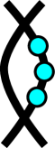
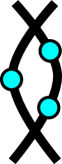
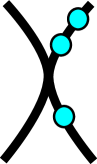
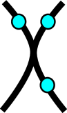
Figure -899: The type $I_{2}$ and type $III$ singular fibers with the possible locations of the three marked points denoted by the blue nodes. Respectively these are $I_{2}^{(ijk)}$, $I_{2}^{(i|jk)}$, $II^{(ijk)}$ and $II^{(i|jk)}$ fibers.

First let us consider the simple case where $s_{1,1}=0$, which is equivalent to stating that $z^{2}\mid{\mathfrak{s}}_{1}$. Then $z^{2}\mid\Delta$ and the singular fiber type, determined by resolving the singularity explicitly as explained in section 3.3, is $I_{2}$. The three rational sections all intersect one of the two components of the $I_{2}$ fiber

$$I_{2}^{(012)}\,:\,(2,1,0,1,0,0,0,0)\,,$$ (4.10)

listed in table 1.

The discriminant can also be enhanced in order by allowing $z$ to divide either of the two polynomials in (4.9). Let us first consider the situation where $s_{6,0}^{2}-4s_{3,0}s_{8,0}$ vanishes. The solution to this equation over this unique factorization domain is given in appendix A and states that

$$s_{6,0} =\mu\sigma_{3}\sigma_{8}$$ (4.11)

$$s_{3,0} =\mu\sigma_{3}^{2}$$ (4.12)

$$s_{8,0} =\mu\sigma_{8}^{2}\,.$$ (4.13)

The discriminant then enhances so that $z^{2}\mid\Delta$. To determine the type of singular fiber here let us consider the equation of the single component of the $I_{1}$ fiber which is being enhanced

$$(s_{3,0}x^{2}+s_{6,0}xy+s_{8,0}y^{2})+xy(s_{7,0}x+s_{9,0}y)=0\,.$$ (4.14)

If $s_{6,0}^{2}-4s_{3,0}s_{8,0}=0$ then the quadratic part of the equation factors into a square which does not divide the cubic terms; this is exactly the form of the equation for a cusp, which is a type $II$ fiber. Therefore we have observed the fiber

$$II_{nc}^{(012)}:\quad\left\{\begin{array}[]{c}(1,1,0,1,0,0,0,0)\cr[-,-,\mu\sigma_{3}^{2},-,2\mu\sigma_{3}\sigma_{8},-,\mu\sigma_{8}^{2},-]\end{array}\right\}\,.$$ (4.15)

from table 1.

Finally we can consider the singular fiber that occurs when the second polynomial in $\Delta$ vanishes: $s_{7,0}^{2}s_{8,0}-s_{6,0}s_{7,0}s_{9,0}+s_{3,0}s_{9,0}^{2}=0$. Appendix A lists four generic solutions of this polynomial, three canonical and one non-canonical, which are:

$$s_{7,0}=s_{9,0}=0$$ (4.16)

$$s_{7,0}=s_{3,0}=0$$ (4.17)

$$s_{8,0}=s_{9,0}=0$$ (4.18)

$$s_{7,0}=\sigma_{1}\sigma_{2}\,,\quad s_{9,0}=\sigma_{1}\sigma_{3}\,,\quad s_{8,0}=\sigma_{3}\sigma_{4}\,,\quad s_{3,0}=\sigma_{2}\sigma_{5}\,,\quad s_{6,0}=\sigma_{2}\sigma_{4}+\sigma_{3}\sigma_{5}\,.$$ (4.19)

Any of the three canonical solutions will remove us from our preferred lop-equivalence class and so we do not consider them as they will give rise to a redundancy of singular fiber types. The only solution to consider therefore is the non-canonical one. The fiber found at this locus is another $I_{2}$ fiber, which can be written as

$$I_{2,nc}:\quad\left\{\begin{array}[]{c}(1,1,0,1,0,0,0,0)\cr[-,-,\sigma_{2}\sigma_{5},-,\sigma_{2}\sigma_{4}+\sigma_{3}\sigma_{5},\sigma_{1}\sigma_{2},\sigma_{3}\sigma_{4},\sigma_{1}\sigma_{3}]\end{array}\right\}\,.$$ (4.20)

Table 1 is then complete up to second order, once we also include the $I_{2}^{(01|2)}$ which was found in the previous section as one of the alternate starting points in the $z\mid{\mathfrak{s}}_{3}$ branch.

4.3 Enhancements from $\operatorname{ord}_{z}(\Delta)=2$

We will now consider the enhancement of the four previously found fibrations which have a discriminant with vanishing order two in $z$. In this section we shall include the details only of those enhancements that have some non-standard behaviour.

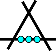
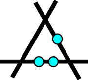
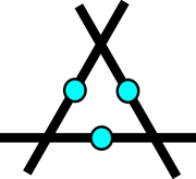
Figure -898: The type $I_{3}$ singular fibers with the locations of the three marked points denoted by the blue nodes. Respectively these are $I_{3}^{(ijk)}$, $I_{3}^{(ij|k)}$ and $I_{3}^{(i|j|k)}$ fibers.

The fibrations $(2,1,0,1,0,0,0,0)$ and $(1,1,1,0,0,0,0,0)$ can contain, respectively, in their discriminants polynomials with five and seven terms. These are not polynomials that are discussed in appendix A as their solutions are not known in full generality. In lieu of a complete solution we consider non-generic but canonical type solutions which allow us to obtain singular fibers of a particular type which would be unobtainable without determining a full, generic solution to these polynomials. The subbranches which follow from enhancements where it has been necessary to consider a non-generic solution will also therefore be non-generic, however all remaining branches are determined in full generality.

4.3.1 Polynomial enhancement in the $z\nmid{\mathfrak{s}}_{3}$ branch

The discriminant of the equation for the $(2,1,0,1,0,0,0,0)$ singular fiber contains the polynomial

$$P=s_{8,0}s_{2,1}^{2}-s_{5,1}s_{6,0}s_{2,1}+s_{1,2}s_{6,0}^{2}+s_{3,0}\left(s_{5,1}^{2}-4s_{1,2}s_{8,0}\right)\,.$$ (4.21)

As the most general solution for this five-term polynomial is not known we propose here two specific solutions. The first is a canonical solution obtained by setting $s_{1,2}=s_{2,1}=s_{5,1}=0$. As a consequence $z^{3}\mid\Delta$ and we find an $I_{3}^{ns(012)}$ singular fiber

$$I_{3}^{ns(012)}\,:\,(3,2,0,2,0,0,0,0)\,.$$ (4.22)

Recalling the split/non-split monodromy distinction in Tate’s algorithm, we see only two components in this singular fiber. One of the fiber curves decomposes when the component of the discriminant, $s_{6,0}^{2}-4s_{3,0}s_{8,0}$ has the form of a perfect, non-zero square.

The second non-general solution to the five-term polynomial we consider here is found by canonically setting $s_{1,2}=0$, and then the five term polynomial reduces to

$$P|_{(s_{1,2}=0)}=s_{2,1}^{2}s_{8,0}-s_{2,1}s_{6,0}s_{5,1}+s_{5,1}^{2}s_{3,0}\,.$$ (4.23)

We notice that we cannot set $s_{3,0}$ to zero because we are in the $z\nmid{\mathfrak{s}}_{3}$ part of the algorithm (and by $\mathbb{Z}_{2}$ symmetry we cannot set to zero $s_{8,0}$ either). Moreover we just considered the canonical solution given by setting $s_{2,1}=s_{5,1}=0$. We are then left with imposing the non-canonical solution given in appendix A

$$s_{2,1}=\sigma_{1}\sigma_{2}\,,\quad s_{5,1}=\sigma_{1}\sigma_{3}\,,\quad s_{8,0}=\sigma_{3}\sigma_{4}\,,\quad s_{3,0}=\sigma_{2}\sigma_{5}\,,\quad s_{6,0}=\sigma_{2}\sigma_{4}+\sigma_{3}\sigma_{5}\,.$$ (4.24)

The resulting singular fiber is then an $I_{3,nc}^{s(012)}$

$$I_{3,nc}^{s(012)}:\quad\left\{\begin{array}[]{c}(3,1,0,1,0,0,0,0)\cr[-,\sigma_{1}\sigma_{2},\sigma_{2}\sigma_{5},\sigma_{1}\sigma_{3},\sigma_{2}\sigma_{4}+\sigma_{3}\sigma_{5},-,\sigma_{3}\sigma_{4},-]\end{array}\right\}\,.$$ (4.25)

4.3.2 Polynomial enhancement in the $z\mid{\mathfrak{s}}_{3}$ branch

The other relevant details we will provide concern enhancements from the singular $I_{2}^{(01|2)}$ which has vanishing orders $(1,1,1,0,0,0,0,0)$. The discriminant contains a seven-term polynomial

$$P =s_{3,1}^{2}s_{5,0}^{2}+s_{7,0}(s_{2,1}^{2}s_{5,0}-s_{1,1}s_{2,1}s_{6,0}+s_{1,1}^{2}s_{7,0})+$$ (4.26)

$$\qquad+s_{3,1}(-s_{2,1}s_{5,0}s_{6,0}+s_{1,1}(s_{6,0}^{2}-2s_{5,0}s_{7,0}))\,.$$

Since a generic solution is not known for this polynomial, we again take advantage of a simple canonical solution given by $s_{1,1}=s_{2,1}=s_{3,1}=0$. We see that $z^{4}\mid\Delta$ and we observe a singular $I_{4}^{ns(01||2)}$

$$I_{4}^{ns(01||2)}\,:\,(2,2,2,0,0,0,0,0)\,.$$ (4.27)

As in the previous case, we notice that the component of the discriminant $s_{6,0}^{2}-4s_{5,0}s_{7,0}$ provides the condition for the split/non-split distinction. If this quantity is a perfect, non-zero square, then applying the solution given in appendix A we have a split $I_{4,nc}^{s(01||2)}$

$$I_{4,nc}^{s(01||2)}:\quad\left\{\begin{array}[]{c}(2,2,2,0,0,0,0,0)\cr[-,-,-,\sigma_{1}\sigma_{3},\sigma_{1}\sigma_{2}+\sigma_{3}\sigma_{4},\sigma_{2}\sigma_{4},-,-]\end{array}\right\}\,.$$ (4.28)

As in the previous subsection, we notice that if we only require $s_{1,1}=0$ the seven term polynomial reduces to the usual three-term one

$$P|_{(s_{1,2}=0)}=s_{5,0}(s_{3,1}^{2}s_{5,0}-s_{3,1}s_{6,0}s_{2,1}+s_{2,1}^{2}s_{7,0})\,.$$ (4.29)

The solution involving setting $s_{5,0}$ to zero in addition to $s_{1,2}$ would give the fibration defined by the vanishing orders $(2,1,1,1,0,0,0,0)$ which is an $I_{3}^{s(01|2)}$ fiber

$$I_{3}^{s(01|2)}\,:\,(2,1,1,1,0,0,0,0)\,.$$ (4.30)

We can also apply the non-canonical solution of appendix A to the three-term component

$$s_{2,1}=\sigma_{1}\sigma_{2}\,,\quad s_{3,1}=\sigma_{1}\sigma_{3}\,,\quad s_{7,0}=\sigma_{3}\sigma_{4}\,,\quad s_{5,0}=\sigma_{2}\sigma_{5}\,,\quad s_{6,0}=\sigma_{2}\sigma_{4}+\sigma_{3}\sigma_{5}\,.$$ (4.31)

Upon substitution we find an $I_{3,nc}^{s(01|2)}$ singular fiber

$$I_{3,nc}^{s(01|2)}:\quad\left\{\begin{array}[]{c}(2,1,1,0,0,0,0,0)\cr[-,\sigma_{1}\sigma_{2},\sigma_{1}\sigma_{3},\sigma_{2}\sigma_{5},\sigma_{2}\sigma_{4}+\sigma_{3}\sigma_{5},\sigma_{3}\sigma_{4},-,-]\end{array}\right\}\,.$$ (4.32)

4.4 Enhancements from $\operatorname{ord}_{z}(\Delta)=3$

We now proceed to consider enhancements of the discriminant starting from the fibers with $\operatorname{ord}_{z}(\Delta)=3$, listed in table 1, and we report here the cases that deserve mention due to some peculiarity. In particular we will consider distinctions between split and non-split singular fibers and an instance where we will need to consider the structure of the algorithm in order not to reproduce singular fibers already obtained.

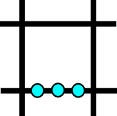
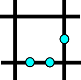
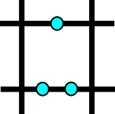
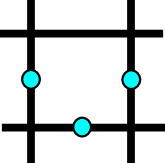
Figure -897: The $I_{4}$ singular fibers and the decorations detailing where the rational sections can intersect. The fibers shown are $I_{4}^{(ijk)}$, $I_{4}^{(ij|k)}$, $I_{4}^{(ij||k)}$ and $I_{4}^{(i|j|k)}$ fibers.

4.4.1 Split/non-split distinction

We recall that in the previous section we found an $I_{3}^{ns(012)}$ singular fiber and we now determine the enhancements of this fiber. The discriminant takes the form

$$\Delta=s_{1,3}s_{3,0}s_{8,0}(s_{6,0}^{2}-4s_{3,0}s_{8,0})(s_{7,0}^{2}s_{8,0}-s_{6,0}s_{7,0}s_{9,0}+s_{3,0}s_{9,0}^{2})z^{3}+\mathcal{O}(z^{4})\,.$$ (4.33)

The simple enhancement $s_{1,3}=0$ will produce an $I_{4}^{ns(012)}$ singular fiber

$$I_{4}^{ns(012)}\,:\,(4,2,0,2,0,0,0,0)\,.$$ (4.34)

As already observed, the discriminant component $s_{6,0}^{2}-4s_{3,0}s_{8,0}$ indicates that when this quantity is a perfect, non-zero square, we obtain the split version of the singular fiber. Applying the solution in appendix A we then find the singular $I_{4,nc}^{s(012)}$

$$I_{4,nc}^{s(012)}:\quad\left\{\begin{array}[]{c}(4,2,0,2,0,0,0,0)\cr[-,-,\sigma_{1}\sigma_{3},-,\sigma_{1}\sigma_{2}+\sigma_{3}\sigma_{4},-,\sigma_{2}\sigma_{4},-]\end{array}\right\}\,.$$ (4.35)

Another instance where the split/non-split distinction arises is in the case of type $IV$ fibers. Consider the singular $III_{nc}^{(012)}$ listed in table 1. This has discriminant

$$\Delta=\mu^{6}\sigma_{3}\sigma_{8}(s_{5,1}\sigma_{3}-s_{2,1}\sigma_{8})(s_{9,0}\sigma_{3}-s_{7,0}\sigma_{8})z^{3}+\mathcal{O}(z^{4})\,.$$ (4.36)

We remark that this was obtained in the algorithm by an application of the non-canonical solution to $s_{6,0}^{2}-4s_{3,0}s_{8,0}=0$ and therefore $\sigma_{3}$ and $\sigma_{8}$ are coprime. Enhancing the discriminant by solving non-canonically the first of the two-term polynomials requires setting

$$s_{5,1}=\xi_{1}\xi_{2},\qquad\sigma_{3}=\xi_{3},\qquad s_{2,1}=\xi_{1}\xi_{3},\qquad\sigma_{8}=\xi_{2}\,.$$ (4.37)

Where coprimality of $(\sigma_{3},\sigma_{8})$ was used in order to set $\xi_{4}=1$. The singular fiber corresponding to this enhancement is a type $IV_{nc^{2}}^{ns(012)}$

$$IV_{nc^{2}}^{ns(012)}:\quad\left\{\begin{array}[]{c}(2,1,0,1,0,0,0,0)\cr[-,\xi_{1}\xi_{3},\mu\xi_{3}^{2},\xi_{1}\xi_{2},2\mu\xi_{2}\xi_{3},-,\mu\xi_{2}^{2},-]\end{array}\right\}\,.$$ (4.38)

Then the discriminant indicates the quantity that needs to be a perfect square in order for the fiber to become a split type $IV_{nc^{3}}^{s(012)}$. This is $\xi_{1}^{2}-4\mu s_{1,2}$, and applying the solution in appendix A we find

$$IV_{nc^{3}}^{s(012)}:\quad\left\{\begin{array}[]{c}(2,1,0,1,0,0,0,0)\cr[\delta_{2}\delta_{4},\xi_{3}(\delta_{1}\delta_{2}+\delta_{3}\delta_{4}),\delta_{1}\delta_{3}\xi_{3}^{2},\xi_{2}(\delta_{1}\delta_{2}+\delta_{3}\delta_{4}),2\delta_{1}\delta_{3}\xi_{2}\xi_{3},-,\delta_{1}\delta_{3}\xi_{2}^{2},-]\end{array}\right\}\,.$$ (4.39)

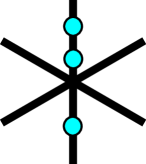
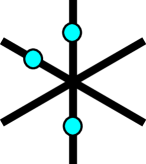
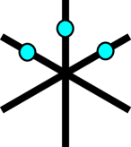
Figure -896: The $IV$ fibers. We denote by the blue nodes the components of the fiber which are intersected by the sections. In the order, the fiber shown are $IV^{(ijk)}$, $IV^{(i|jk)}$ and $IV^{(i|j|k)}$ fibers.

4.4.2 Commutative enhancement structure of the algorithm

We consider enhancements from the $III_{nc^{2}}^{(1|02)}$ fiber type. This was found by applying twice the solutions in appendix A. Schematically

$$I_{1}^{(012)}\longrightarrow I_{2,nc}^{(1|02)}\longrightarrow III_{nc^{2}}^{(1|02)}\,.$$ (4.40)

Noting that in the last step a coprimality condition had to be imposed, the discriminant of this singular fiber takes the form

$$\Delta=(s_{1,1}^{3}\xi_{2}^{6}\xi_{3}^{6}\xi_{4}^{6})z^{3}+\mathcal{O}(z^{4})\,.$$ (4.41)

We see that requiring the vanishing of any of the $\xi_{i}$ would imply setting to zero two among $s_{7,0},s_{9,0},s_{3,0},s_{8,0}$, but we are not allowing the vanishing of any of the those sections to remain in our lop equivalence class or because we are in the $z\nmid{\mathfrak{s}}_{3}$ branch of the algorithm. Moreover, we have considered the case $s_{1,1}=0$ in another part of the algorithm (specifically in going $I_{1}^{(012)}\rightarrow I_{2}^{(012)}$). We can therefore conclude that all the enhancements would just reproduce singular fibers found in other parts of the algorithm. The order in which the enhancements are carried out is of no importance, but it is crucial, in particular with non-canonical fibers, to keep track of which enhancements would reproduce fiber types already obtained.

4.5 Enhancements from $\operatorname{ord}_{z}(\Delta)=4$

In this section we will proceed with the algorithm by again mentioning only enhancements which require comment. In particular we will deal with the structure of obstructions to full generality due to the complexity of polynomials in the discriminant, we will encounter the distinction between split and semi-split fibers for $I_{0}^{*}$ and we will provide details for one of the $I_{5,nc^{3}}$, obtained by solving non-canonically polynomials in the discriminant three times.

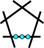
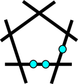
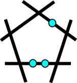
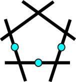
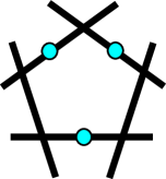
Figure -895: The $I_{5}$ singular fibers. The possible intersections of the sections with the singular fibers are denoted by the positions of the blue nodes. The fibers shown in the first row are $I_{5}^{(ijk)}$, $I_{5}^{(ij|k)}$ and $I_{5}^{(ij||k)}$, whereas the fibers shown in the second row are, respectively, $I_{5}^{(i|j|k)}$ and $I_{5}^{(i|j||k)}$.

4.5.1 Obstruction from polynomial enhancement

At vanishing order of the discriminant $\operatorname{ord}_{z}(\Delta)=4$ we find again the two obstructions to full generality encountered at $\operatorname{ord}_{z}(\Delta)=2$, i.e. the same five-term and seven-term polynomials. These come up respectively in the discriminant of the singular fibers $I_{4}^{ns(012)}$ and $I_{4}^{ns(01||2)}$, and will in fact be present at every even vanishing order in the discriminants of $I_{2n}^{ns(012)}$ and $I_{2n}^{ns(01|^{n}2)}$. We therefore review the singular fibers that we obtain from the enhancements. More details can be found in section 4.3.

The discriminant of the singular fiber $I_{4}^{ns(012)}:(4,2,0,2,0,0,0,0)$ contains a component

$$\Delta\supset P=s_{8,0}s_{2,2}^{2}-s_{5,2}s_{6,0}s_{2,2}+s_{1,4}s_{6,0}^{2}+s_{3,0}\left(s_{5,2}^{2}-4s_{1,4}s_{8,0}\right)\,.$$ (4.42)

As in section 4.3 we consider two specific solutions. The first one consists of setting $s_{1,4}=s_{2,2}=s_{5,2}=0$. This gives the singular fiber $I_{5}^{ns(012)}$

$$I_{5}^{ns(012)}\,:\,(5,3,0,3,0,0,0,0)\,.$$ (4.43)

Upon imposing the perfect square condition $s_{6,0}^{2}-4s_{3,0}s_{8,0}=p^{2}$ we find the singular fiber $I_{5}^{s(012)}$. Alternatively, we set $s_{1,4}=0$ and we solve non-canonically, as in appendix A, the resulting three-term polynomial polynomial

$$P|_{(s_{1,4}=0)}=s_{2,2}^{2}s_{8,0}-s_{2,2}s_{6,0}s_{5,2}+s_{5,2}^{2}s_{3,0}\,.$$ (4.44)

This gives the non-canonical singular fiber $I_{5,nc}^{s(012)}$

$$I_{5,nc}^{s(012)}:\quad\left\{\begin{array}[]{c}(5,2,0,2,0,0,0,0)\cr[-,\sigma_{1}\sigma_{2},\sigma_{2}\sigma_{5},\sigma_{1}\sigma_{3},\sigma_{2}\sigma_{4}+\sigma_{3}\sigma_{5},-,\sigma_{3}\sigma_{4},-]\end{array}\right\}\,.$$ (4.45)

The second obstruction that we encounter is, again, the seven-term polynomial in the discriminant of the singular $I_{4}^{ns(01||2)}$

$$\Delta\supset P =s_{3,2}^{2}s_{5,0}^{2}+s_{7,0}(s_{2,2}^{2}s_{5,0}-s_{1,2}s_{2,2}s_{6,0}+s_{1,2}^{2}s_{7,0})+$$ (4.46)

$$\qquad+s_{3,2}(-s_{2,2}s_{5,0}s_{6,0}+s_{1,2}(s_{6,0}^{2}-2s_{5,0}s_{7,0}))\,.\$$

The canonical solution that we consider requires $s_{1,2}=s_{2,2}=s_{3,2}=0$. This gives a singular $I_{6}^{ns(01|||2)}$

$$I_{6}^{ns(01|||2)}\,:\,(3,3,3,0,0,0,0,0)\,.$$ (4.47)

The split version $I_{6}^{s(01|||2)}$ is found upon imposing that $s_{6,0}^{2}-4s_{5,0}s_{7,0}$ is a perfect, non-zero square. We can also consider the solution where $s_{1,2}=0$ and the three-term polynomial component of the resulting polynomial is solved non-canonically. This enhancement now produces an $I_{5,nc}^{s(01||2)}$, but this is just a non-generic specialization of one of the $I_{5,nc^{2}}^{s(01||2)}$ fibers also found in the algorithm and so we do not consider it further.

4.5.2 Split/semi-split Distinction

The split/semi-split distinction arises for singular fibers of Kodaira type $I_{0}^{*}$. The example we provide concerns the possible enhancement of the canonical type $IV^{s(01|2)}$, which was found schematically by

$$I_{2}^{(01|2)}\longrightarrow I_{3}^{s(01|2)}\longrightarrow IV^{s(01|2)}\,.$$ (4.48)

The discriminant takes a rather simple form

$$\Delta=s_{2,1}s_{7,0}s_{8,0}z^{4}+\mathcal{O}(z^{5})\,.$$ (4.49)

The enhancement we will consider here is when $s_{2,1}=0$. As a consequence $z^{2}\mid{\mathfrak{s}}_{2}$ and $z^{6}\mid\Delta$. This way we have found the semi-split $I_{0}^{*ss(01|2)}$

$$I_{0}^{*ss(01|2)}\,:\,(2,2,1,1,1,0,0,0)\,.\,$$ (4.50)

In order for one of the curves of the $I_{0}^{*ss(01|2)}$ to split into two separate non-intersecting components, we need to satisfy a perfect square condition for the quantity $s_{5,1}^{2}-4s_{1,2}s_{8,0}$. Following appendix A we find the split $I_{0,nc}^{*s(01|2)}$

$$I_{0,nc}^{*s(01|2)}:\quad\left\{\begin{array}[]{c}(2,2,1,1,1,0,0,0)\cr[\sigma_{1}\sigma_{3},-,-,\sigma_{1}\sigma_{2}+\sigma_{3}\sigma_{4},-,-,\sigma_{2}\sigma_{4},-]\end{array}\right\}\,.$$ (4.51)

4.5.3 A thrice non-canonical $I_{5}$

In this section we provide details for an $I_{5,nc^{3}}^{s(0|1||2)}$. This singular fiber is observed in the algorithm by schematically enhancing

$$I_{2}^{(01|2)}\longrightarrow I_{3,nc}^{s(0|1|2)}\longrightarrow I_{4,nc^{2}}^{s(0|1|2)}\longrightarrow I_{5,nc^{3}}^{s(0|1||2)}\,.$$ (4.52)

All the three arrows represent non-canonical enhancements. In particular enhancing from $I_{2}^{(01|2)}$ to $I_{3,nc}^{s(0|1|2)}$ requires solving a three-term polynomial present in the discriminant. This is $\Delta\supset(s_{8,0}^{2}s_{7,0}-s_{8,0}s_{6,0}s_{9,0}+s_{9,0}^{2}s_{5,0})$, which is solved by requiring

$$s_{8,0}=\sigma_{1}\sigma_{2},\quad s_{9,0}=\sigma_{1}\sigma_{3},\quad s_{7,0}=\sigma_{3}\sigma_{4},\quad s_{5,0}=\sigma_{2}\sigma_{5},\quad s_{6,0}=\sigma_{2}\sigma_{4}+\sigma_{3}\sigma_{5}\,.$$ (4.53)

Note that this solution implies that $(\sigma_{2},\sigma_{3})$ are coprime. This gives an $I_{3,nc}^{s(0|1|2)}$. Looking at the discriminant of this singular fiber we see that one of the components is $\Delta\supset(\sigma_{3}^{2}s_{1,1}-\sigma_{2}\sigma_{3}s_{2,1}+\sigma_{2}^{2}s_{3,1})$. We apply again the same solution to this three-term polynomial

$$\sigma_{3}=\xi_{2},\quad\sigma_{2}=\xi_{3},\quad s_{1,1}=\xi_{3}\xi_{4},\quad s_{3,1}=\xi_{2}\xi_{5},\quad s_{2,1}=\xi_{2}\xi_{4}+\xi_{3}\xi_{5}\,.$$ (4.54)

Where we used that $(\sigma_{2},\sigma_{3})$ are coprime to set $\xi_{1}=1$. We have now enhanced the singular fiber to an $I_{4,nc^{2}}^{s(0|1|2)}$. To obtain the thrice non-canonical $I_{5}$ we now consider the two-term polynomial contained in the discriminant at fourth order: $\Delta\supset(\sigma_{4}\xi_{4}-\sigma_{5}\xi_{5})$. Applying the non-canonical solution in appendix A

$$\sigma_{4}=\delta_{1}\delta_{2},\quad\xi_{4}=\delta_{3}\delta_{4},\quad\sigma_{5}=\delta_{1}\delta_{3},\quad\xi_{5}=\delta_{2}\delta_{4}\,.$$ (4.55)

We have now reached the singular fiber $I_{5,nc^{3}}^{s(0|1||2)}$

$$I_{5,nc^{3}}^{*s(0|2||1)}:\quad\left\{\begin{array}[]{c}(1,1,1,0,0,0,0,0)\cr[\xi_{3}\delta_{3}\delta_{4},\delta_{4}(\delta_{3}\xi_{2}+\delta_{2}\xi_{3}),\xi_{2}\delta_{2}\delta_{4},\xi_{3}\delta_{1}\delta_{3},\delta_{1}(\delta_{2}\xi_{3}+\delta_{3}\xi_{2}),\delta_{1}\delta_{2}\xi_{2},\sigma_{1}\xi_{3},\sigma_{1}\xi_{2}]\end{array}\right\}\,.$$ (4.56)

5 $U(1)$ Charges of $SU(5)$ Fibers

In section 4 a variety of different, canonical and non-canonical, $I_{5}$ type singular fibers were found, and are listed in table 3. As elliptic fibrations with $SU(5)$ singular fibers are phenomenologically interesting in this section the $U(1)$ charges of the matter loci are determined for the $I_{5}$ fibers obtained, which lie in the chosen lop-equivalence class. The $U(1)$ charges are calculated from the intersection number of the matter curve with the Shioda mapped rational section, as explained in section 3.3. For the canonical $I_{5}$ singular fibers we find, as expected, the same results that were found from the study of toric tops. Details of the relationship between the canonical models and the $SU(5)$ top models and their charges as found in [38] are given. In the algorithm a number of non-canonical models which, as far as the authors are aware have not been seen before, were found, some of which can realize two or three distinctly charged ${\bf 10}$ matter curves, potentially a desirable feature, also some models realize as many as seven differently charged ${\bf 5}$ matter curves, which are of some interest in light of the phenomenological study in [33].

5.1 Canonical $I_{5}$ Models

The $U(1)$ charges of the canonical models are found in table 5. Models with these particular $U(1)$ charges are well-studied in the literature. In this subsection we provide a short comparison to the known toric constructions from tops [43] , which were constructed with two extra sections in [38, 30, 34, 36].

The toric tops as extracted from [38] are also given by vanishing orders of the coefficients of the cubic polynomial (2.1) and are related to what we called canonical models. In order to see this we need to perform a series of lop transformations to bring them to the equivalence class of singular fibers considered in this paper. Section 3.2 contains the details of the lop transformations. All the tops were found as part of the algorithm and exhaust the canonical models. The $U(1)$ charges of the matter content matched the results found here identically for what was called tops 1 and 2, whereas for tops 3 and 4 a different linear combination of the $U(1)$ charges was used. The details of this linear combination are given in terms of our choice of $U(1)$ generators.

$$\begin{array}[]{|c|c|c|c|}\hline\cr\text{Fiber}&\text{Model}&\text{Matter Locus}&\text{Matter}\cr\hline\cr I_{5}^{s(0|1||2)}&\begin{array}[]{c}(2,2,2,1,0,0,1,0)\cr\end{array}&\begin{array}[]{c}s_{1,2}\cr s_{6,0}\cr s_{7,0}\cr s_{9,0}\cr s_{6,0}s_{8,1}-s_{5,1}s_{9,0}\cr s_{3,2}s_{6,0}^{2}-s_{2,2}s_{6,0}s_{7,0}+s_{1,2}s_{7,0}^{2}\cr\end{array}&\begin{array}[]{c}{\bf 5}_{3,1}\oplus{\bf\overline{5}}_{-3,-1}\cr{\bf 10}_{1,2}\oplus{\bf\overline{10}}_{-1,-2}\cr{\bf 5}_{3,-4}\oplus{\bf\overline{5}}_{-3,4}\cr{\bf 5}_{3,6}\oplus{\bf\overline{5}}_{-3,-6}\cr{\bf 5}_{-2,1}\oplus{\bf\overline{5}}_{2,-1}\cr{\bf 5}_{-2,-4}\oplus{\bf\overline{5}}_{2,4}\cr\end{array}\cr\hline\cr I_{5}^{s(01||2)}&\begin{array}[]{c}(3,2,2,1,0,0,0,0)\cr\end{array}&\begin{array}[]{c}s_{6,0}\cr s_{7,0}\cr s_{8,0}\cr s_{1,3}s_{6,0}-s_{2,2}s_{5,1}\cr s_{3,2}s_{6,0}-s_{2,2}s_{7,0}\cr s_{6,0}s_{9,0}-s_{7,0}s_{8,0}\cr\end{array}&\begin{array}[]{c}{\bf 10}_{-1,0}\oplus{\bf\overline{10}}_{1,0}\cr{\bf 5}_{2,-1}\oplus{\bf\overline{5}}_{-2,1}\cr{\bf 5}_{-3,-1}\oplus{\bf\overline{5}}_{3,1}\cr{\bf 5}_{2,0}\oplus{\bf\overline{5}}_{-2,0}\cr{\bf 5}_{-3,0}\oplus{\bf\overline{5}}_{3,0}\cr{\bf 5}_{2,1}\oplus{\bf\overline{5}}_{-2,-1}\cr\end{array}\cr\hline\cr I_{5}^{s(0|1|2)}&\begin{array}[]{c}(3,2,1,1,0,0,1,0)\cr\end{array}&\begin{array}[]{c}s_{3,1}\cr s_{6,0}\cr s_{7,0}\cr s_{9,0}\cr s_{5,1}s_{9,0}-s_{6,0}s_{8,1}\cr s_{3,1}s_{5,1}^{2}-s_{2,2}s_{5,1}s_{6,0}+s_{1,3}s_{6,0}^{2}\cr\end{array}&\begin{array}[]{c}{\bf 5}_{-3,1}\oplus{\bf\overline{5}}_{3,-1}\cr{\bf 10}_{-1,2}\oplus{\bf\overline{10}}_{1,-2}\cr{\bf 5}_{2,-4}\oplus{\bf\overline{5}}_{-2,4}\cr{\bf 5}_{2,6}\oplus{\bf\overline{5}}_{-2,-6}\cr{\bf 5}_{2,1}\oplus{\bf\overline{5}}_{-2,-1}\cr{\bf 5}_{-3,-4}\oplus{\bf\overline{5}}_{3,4}\cr\end{array}\cr\hline\cr I_{5}^{s(01|2)}&\begin{array}[]{c}(4,2,1,2,0,0,0,0)\cr\end{array}&\begin{array}[]{c}s_{3,1}\cr s_{6,0}\cr s_{7,0}\cr s_{8,0}\cr s_{6,0}s_{9,0}-s_{7,0}s_{8,0}\cr s_{1,4}s_{6,0}^{2}-s_{2,2}s_{5,2}s_{6,0}+s_{2,2}^{2}s_{8,0}\cr\end{array}&\begin{array}[]{c}{\bf 5}_{4,0}\oplus{\bf\overline{5}}_{-4,0}\cr{\bf 10}_{-2,0}\oplus{\bf\overline{10}}_{2,0}\cr{\bf 5}_{-1,1}\oplus{\bf\overline{5}}_{1,-1}\cr{\bf 5}_{4,1}\oplus{\bf\overline{5}}_{-4,-1}\cr{\bf 5}_{-1,-1}\oplus{\bf\overline{5}}_{1,1}\cr{\bf 5}_{-1,0}\oplus{\bf\overline{5}}_{1,0}\cr\end{array}\cr\hline\cr\end{array}$$

Table 5: $U(1)$ charges of the canonical $I_{5}$ models from table 3.

In table 6 the tops are listed with the numbering and vanishing orders as in appendix A of [38](polygon 5), the lop equivalent models as found in Tate’s algorithm and details for the linear combination of the $U(1)$ charges for top 3 and top 4.

Top	Fiber	Vanishing Orders	Lop-equivalent model	$U(1)$ Linear Combination
Top 1	$I_{5}^{s(0|1|2)}$	$(2,2,2,0,0,1,0,0)$	$(3,2,1,1,0,0,1,0)$	-
Top 2	$I_{5}^{s(0|1||2)}$	$(1,2,3,0,0,1,0,0)$	$(2,2,2,1,0,0,1,0)$	-
Top 3	$I_{5}^{s(01||2)}$	$(1,1,2,0,0,2,0,0)$	$(3,2,2,1,0,0,0,0)$	$\begin{array}[]{c}u_{1}=-\text{w}_{1}\cr u_{2}=\frac{1}{5}(\text{w}_{2}-\text{w}_{1})\end{array}$
Top 4	$I_{5}^{s(01|2)}$	$(1,1,1,0,0,2,0,1)$	$(4,2,1,2,0,0,0,0)$	$\begin{array}[]{c}u_{1}=-\text{w}_{1}\cr u_{2}=\frac{1}{5}(\text{w}_{2}-\text{w}_{1})\end{array}$

Table 6: The lop-equivalent models of the four tops from [38]. The linear combination of the $U(1)$ charges gives the charges found in table 5, $u_{1}$ and $u_{2}$, in terms of the $U(1)$ charges of the top model, w₁ and w₂. The reason the charges of tops 3 and 4 differ is because the lop translation involves the $\mathbb{Z}_{2}$ symmetry, which exchanges two of the marked points.

5.2 Non-canonical $I_{5}$ Models

Listed in tables 8, 9 and 10 are the $U(1)$ charges of the, respectively once, twice, and thrice, non-canonical $I_{5}$ models found in the algorithm. The $U(1)$ charge generators are given by the Shioda map, as described in section 3.3, where the zero-section of the fibration corresponds to the divisor $l_{1}=0$ after the $\mathbb{P}^{2}$ fibration ambient space has been blown up into $dP_{2}$. As opposed to the canonical models the majority of the models tabulated in this section were previously unknown. Some of these models appear to have interesting properties for phenomenology, such as the above noted multiple differently charged ${\bf 10}$ and ${\bf 5}$ curves.

While Tate’s algorithm provides a generic procedure there are some caveats that were introduced in the application of it studied in this paper. There are situations where we were not able to solve for the enhancement locus in the discriminant to a reasonable degree of generality. In these cases we have sometimes, as discussed in section 4, used a less generic solution where it was obtainable in such a way that it did not lead to obvious irregularities with the model. In cases where no such solution was obtained we have left that particular subbranch of the Tate tree unexplored.

Throughout the application of Tate’s algorithm the fibrations have remained inside the chosen lop-equivalence class and so each each model in these tables then represents an entire lop-orbit of fibrations. The $\mathbb{Z}_{2}$ symmetry which acts inside this orbit interchanges two of the three marked points of the fibration, which correspond, in the $dP_{2}$ hypersurface, to the exchange of $l_{1}$ and $l_{2}$. As the $U(1)$ charges are computed from a Shioda map where the zero-section is taken to be $l_{1}=0$ the $U(1)$ charges are rewritten as a linear combination under this symmetry in an identical manner to the linear combinations occurring in the tops in table 6.

One may point out the surprising paucity of non-minimal matter loci in these models with highly specialised coefficients. In the fibrations which are at least twice non-canonical there can occur polynomial enhancement loci where some of the terms in the solutions (as given in appendix A) are fixed by a coprimality condition coming from a previously solved polynomial. Were these terms not fixed to unity by the algorithm then they would contribute non-minimal loci to the fibrations.

In [38, 30] there were listed tops corresponding to an $SU(4)$ non-abelian singularity with two additional rational sections, and it was noted that one expects multiple 10 matter curves where these tops are specialized with some non-generic coefficients of the defining polynomial, and such a model, which realizes multiple ${\bf 10}$ curves, was constructed there from the $SU(4)$ tops. Included in table 7 are the relations (via the lops) between these $SU(4)$ tops and the $SU(4)$ canonical models which underlie the once non-canonical $SU(5)$ models obtained in the algorithm.

Top Model	Fiber	Vanishing Orders	Lop-equivalent Model
Top 1	$I_{4}^{(0|1|2)}$	$(1,1,2,0,0,1,0,0)$	$(2,1,1,1,0,0,1,0)$
Top 2	$I_{4}^{(01||2)}$	$(0,1,2,0,0,2,0,0)$	$(2,2,2,1,0,0,0,0)$
Top 3	$I_{4}^{(01|2)}$	$(1,1,1,0,0,1,0,1)$	$(3,2,1,1,0,0,0,0)$
Top 4	$I_{4}^{(01||2)}$	$(0,1,2,0,0,1,0,1)$	$(2,2,2,1,0,0,0,0)$
Top 5	$I_{4}^{(01|2)}$	$(0,0,1,0,0,2,0,1)$	$(3,2,1,1,0,0,0,0)$

Table 7: The $SU(4)$ tops associated to polygon 5 in appendix B of [38] are related to the canonical $I_{4}$ models listed in table 2 by lop-equivalence.

Note that for $SU(4)$ top 4 is lop equivalent to top 2 and top 5 is lop equivalent top 3, and their $U(1)$ charges, as listed in appendix B of [38], can be written as a linear combination of the lop-equivalent model.

$$\begin{array}[]{|c|c|c|c|}\hline\cr\text{Fiber}&\text{Model}&\text{Matter Locus}&\text{Matter}\cr\hline\cr I_{5}^{s(0|1||2)}&\begin{array}[]{c}(2,2,2,0,0,0,0,0)\cr[-,-,-,\sigma_{2}\sigma_{5},\sigma_{2}\sigma_{4}+\sigma_{3}\sigma_{5},\sigma_{3}\sigma_{4},\sigma_{1}\sigma_{2},\sigma_{1}\sigma_{3}]\end{array}&\begin{array}[]{c}\sigma_{1}\cr\sigma_{3}\cr\sigma_{4}\cr\sigma_{2}\sigma_{4}-\sigma_{3}\sigma_{5}\cr(\ref{NL1})\cr(\ref{NL2})\cr(\ref{NL3})\cr\end{array}&\begin{array}[]{c}{\bf 5}_{-3,-6}\oplus{\bf\overline{5}}_{3,6}\cr{\bf 5}_{2,-6}\oplus{\bf\overline{5}}_{-2,6}\cr{\bf 5}_{-3,4}\oplus{\bf\overline{5}}_{3,-4}\cr{\bf 10}_{-1,-2}\oplus{\bf\overline{10}}_{1,2}\cr{\bf 5}_{-3,-1}\oplus{\bf\overline{5}}_{3,1}\cr{\bf 5}_{2,-1}\oplus{\bf\overline{5}}_{-2,1}\cr{\bf 5}_{2,4}\oplus{\bf\overline{5}}_{-2,-4}\cr\end{array}\cr\hline\cr I_{5}^{s(0|1|2)}&\begin{array}[]{c}(2,1,1,1,0,0,1,0)\cr[\sigma_{1}\sigma_{3},\sigma_{1}\sigma_{2},-,\sigma_{3}\sigma_{4},\sigma_{2}\sigma_{4},-,-,-]\end{array}&\begin{array}[]{c}\sigma_{2}\cr\sigma_{4}\cr s_{7,0}\cr s_{9,0}\cr\sigma_{4}s_{3,1}-\sigma_{1}s_{7,0}\cr\sigma_{2}s_{8,1}-\sigma_{3}s_{9,0}\cr(\ref{NL4})\cr\end{array}&\begin{array}[]{c}{\bf 10}_{1,-2}\oplus{\bf\overline{10}}_{-1,2}\cr{\bf 10}_{1,3}\oplus{\bf\overline{10}}_{-1,-3}\cr{\bf 5}_{-2,4}\oplus{\bf\overline{5}}_{2,-4}\cr{\bf 5}_{-2,-6}\oplus{\bf\overline{5}}_{2,6}\cr{\bf 5}_{3,-1}\oplus{\bf\overline{5}}_{-3,1}\cr{\bf 5}_{3,4}\oplus{\bf\overline{5}}_{-3,-4}\cr{\bf 5}_{-2,-1}\oplus{\bf\overline{5}}_{2,1}\cr\end{array}\cr\hline\cr I_{5}^{s(0|1||2)}&\begin{array}[]{c}(2,1,1,1,0,0,1,0)\cr[-,\sigma_{1}\sigma_{2},\sigma_{1}\sigma_{3},-,\sigma_{2}\sigma_{4},\sigma_{3}\sigma_{4},-,-]\end{array}&\begin{array}[]{c}\sigma_{2}\cr\sigma_{3}\cr\sigma_{4}\cr s_{9,0}\cr\sigma_{4}s_{1,2}-\sigma_{1}s_{5,1}\cr\sigma_{2}\sigma_{4}s_{8,1}-s_{5,1}s_{9,0}\cr(\ref{NL5})\cr\end{array}&\begin{array}[]{c}{\bf 10}_{-1,-2}\oplus{\bf\overline{10}}_{1,2}\cr{\bf 5}_{-3,4}\oplus{\bf\overline{5}}_{3,-4}\cr{\bf 10}_{-1,3}\oplus{\bf\overline{10}}_{1,-3}\cr{\bf 5}_{-3,-6}\oplus{\bf\overline{5}}_{3,6}\cr{\bf 5}_{-3,-1}\oplus{\bf\overline{5}}_{3,1}\cr{\bf 5}_{2,4}\oplus{\bf\overline{5}}_{-2,-4}\cr{\bf 5}_{2,-1}\oplus{\bf\overline{5}}_{-2,1}\cr\end{array}\cr\hline\cr I_{5}^{s(1|0|2)}&\begin{array}[]{c}(3,2,1,1,0,0,0,0)\cr[-,-,-,-,\sigma_{1}\sigma_{2},\sigma_{1}\sigma_{3},\sigma_{2}\sigma_{4},\sigma_{3}\sigma_{4}]\end{array}&\begin{array}[]{c}\sigma_{1}\cr\sigma_{2}\cr\sigma_{3}\cr\sigma_{4}\cr s_{3,1}\cr(\ref{NL6})\cr(\ref{NL7})\cr\end{array}&\begin{array}[]{c}{\bf 10}_{-2,2}\oplus{\bf\overline{10}}_{2,-2}\cr{\bf 10}_{3,2}\oplus{\bf\overline{10}}_{-3,-2}\cr{\bf 5}_{-1,6}\oplus{\bf\overline{5}}_{1,-6}\cr{\bf 5}_{4,6}\oplus{\bf\overline{5}}_{-4,-6}\cr{\bf 5}_{4,1}\oplus{\bf\overline{5}}_{-4,-1}\cr{\bf 5}_{-1,1}\oplus{\bf\overline{5}}_{1,-1}\cr{\bf 5}_{-1,-4}\oplus{\bf\overline{5}}_{1,4}\cr\end{array}\cr\hline\cr I_{5}^{s(01|2)}&\begin{array}[]{c}(3,2,1,1,0,0,0,0)\cr[\sigma_{2}\sigma_{5},\sigma_{2}\sigma_{4}+\sigma_{3}\sigma_{5},\sigma_{3}\sigma_{4},\sigma_{1}\sigma_{2},\sigma_{1}\sigma_{3},-,-,-]\end{array}&\begin{array}[]{c}\sigma_{1}\cr\sigma_{3}\cr\sigma_{4}\cr s_{7,0}\cr s_{8,0}\cr\sigma_{1}\sigma_{3}s_{9,0}-s_{7,0}s_{8,0}\cr(\ref{NL8})\cr\end{array}&\begin{array}[]{c}{\bf 10}_{2,0}\oplus{\bf\overline{10}}_{-2,0}\cr{\bf 10}_{-3,0}\oplus{\bf\overline{10}}_{3,0}\cr{\bf 5}_{-4,0}\oplus{\bf\overline{5}}_{4,0}\cr{\bf 5}_{1,-1}\oplus{\bf\overline{5}}_{-1,1}\cr{\bf 5}_{-4,-1}\oplus{\bf\overline{5}}_{4,1}\cr{\bf 5}_{1,1}\oplus{\bf\overline{5}}_{-1,-1}\cr{\bf 5}_{1,0}\oplus{\bf\overline{5}}_{-1,0}\cr\end{array}\cr\hline\cr I_{5}^{s(1|02)}&\begin{array}[]{c}(4,2,0,2,0,0,0,0)\cr[-,-,\sigma_{3}\sigma_{4},-,\sigma_{2}\sigma_{4}+\sigma_{3}\sigma_{5},\sigma_{1}\sigma_{3},\sigma_{2}\sigma_{5},\sigma_{1}\sigma_{2}]\end{array}&\begin{array}[]{c}\sigma_{1}\cr\sigma_{2}\cr\sigma_{3}\cr\sigma_{4}\cr\sigma_{5}\cr\sigma_{2}\sigma_{4}-\sigma_{3}\sigma_{5}\cr(\ref{NL9})\cr(\ref{NL10})\cr\end{array}&\begin{array}[]{c}{\bf 5}_{0,6}\oplus{\bf\overline{5}}_{0,-6}\cr{\bf 5}_{1,6}\oplus{\bf\overline{5}}_{-1,-6}\cr{\bf 5}_{-1,1}\oplus{\bf\overline{5}}_{1,-1}\cr{\bf 5}_{1,1}\oplus{\bf\overline{5}}_{-1,-1}\cr{\bf 5}_{-1,-4}\oplus{\bf\overline{5}}_{1,4}\cr{\bf 10}_{0,2}\oplus{\bf\overline{10}}_{0,-2}\cr{\bf 5}_{0,-4}\oplus{\bf\overline{5}}_{0,4}\cr{\bf 5}_{0,1}\oplus{\bf\overline{5}}_{0,-1}\cr\end{array}\cr\hline\cr I_{5}^{s(012)}&\begin{array}[]{c}(5,2,0,2,0,0,0,0)\cr[-,\sigma_{1}\sigma_{2},\sigma_{2}\sigma_{5},\sigma_{1}\sigma_{3},\sigma_{2}\sigma_{4}+\sigma_{3}\sigma_{5},-,\sigma_{3}\sigma_{4},-]\end{array}&\begin{array}[]{c}\sigma_{2}\cr\sigma_{3}\cr\sigma_{4}\cr\sigma_{5}\cr\sigma_{2}\sigma_{4}-\sigma_{3}\sigma_{5}\cr\sigma_{3}s_{7,0}-\sigma_{2}s_{9,0}\cr\sigma_{4}s_{7,0}-\sigma_{5}s_{9,0}\cr(\ref{NL11})\cr\end{array}&\begin{array}[]{c}{\bf 5}_{-1,0}\oplus{\bf\overline{5}}_{1,0}\cr{\bf 5}_{1,1}\oplus{\bf\overline{5}}_{-1,-1}\cr{\bf 5}_{-1,-1}\oplus{\bf\overline{5}}_{1,1}\cr{\bf 5}_{1,0}\oplus{\bf\overline{5}}_{-1,0}\cr{\bf 10}_{0,0}\oplus{\bf\overline{10}}_{0,0}\cr{\bf 5}_{0,-1}\oplus{\bf\overline{5}}_{0,1}\cr{\bf 5}_{0,1}\oplus{\bf\overline{5}}_{0,-1}\cr{\bf 5}_{0,0}\oplus{\bf\overline{5}}_{0,0}\cr\end{array}\cr\hline\cr\end{array}$$

Table 8: $U(1)$ charges of the once non-canonical $I_{5}$ models from table 3.

$$\begin{array}[]{|c|c|c|c|}\hline\cr\text{Fiber}&\text{Model}&\text{Matter Locus}&\text{Matter}\cr\hline\cr I_{5}^{s(01||2)}&\begin{array}[]{c}(2,2,2,0,0,0,0,0)\cr[\xi_{3}\xi_{4},\xi_{2}\xi_{4}+\xi_{3}\xi_{5},\xi_{2}\xi_{5},\sigma_{3}\xi_{3},\sigma_{2}\xi_{3}+\sigma_{3}\xi_{2},\sigma_{2}\xi_{2},-,-]\end{array}&\begin{array}[]{c}\xi_{2}\cr\sigma_{2}\cr\sigma_{2}\xi_{3}-\sigma_{3}\xi_{2}\cr\sigma_{2}\xi_{4}-\sigma_{3}\xi_{5}\cr\xi_{2}s_{8,0}-\xi_{3}s_{9,0}\cr\sigma_{2}s_{8,0}-\sigma_{3}s_{9,0}\cr(\ref{NL12})\cr\end{array}&\begin{array}[]{c}{\bf 5}_{3,-1}\oplus{\bf\overline{5}}_{-3,1}\cr{\bf 5}_{-2,1}\oplus{\bf\overline{5}}_{2,-1}\cr{\bf 10}_{1,0}\oplus{\bf\overline{10}}_{-1,0}\cr{\bf 5}_{3,0}\oplus{\bf\overline{5}}_{-3,0}\cr{\bf 5}_{3,1}\oplus{\bf\overline{5}}_{-3,-1}\cr{\bf 5}_{-2,-1}\oplus{\bf\overline{5}}_{2,1}\cr{\bf 5}_{-2,0}\oplus{\bf\overline{5}}_{2,0}\cr\end{array}\cr\hline\cr I_{5}^{s(0|1||2)}&\begin{array}[]{c}(2,1,1,1,0,0,0,0)\cr[-,\sigma_{1}\xi_{3},\sigma_{1}\xi_{2},-,\sigma_{4}\xi_{3},\sigma_{4}\xi_{2},\xi_{3}\xi_{4},\xi_{2}\xi_{4}]\end{array}&\begin{array}[]{c}\xi_{2}\cr\xi_{3}\cr\xi_{4}\cr\sigma_{4}\cr(\ref{NL13})\cr(\ref{NL14})\cr(\ref{NL15})\cr\end{array}&\begin{array}[]{c}{\bf 5}_{2,-6}\oplus{\bf\overline{5}}_{-2,6}\cr{\bf 10}_{-1,-2}\oplus{\bf\overline{10}}_{1,2}\cr{\bf 5}_{-3,-6}\oplus{\bf\overline{5}}_{3,6}\cr{\bf 10}_{-1,3}\oplus{\bf\overline{10}}_{1,-3}\cr{\bf 5}_{2,-1}\oplus{\bf\overline{5}}_{-2,1}\cr{\bf 5}_{-3,-1}\oplus{\bf\overline{5}}_{3,1}\cr{\bf 5}_{2,4}\oplus{\bf\overline{5}}_{-2,-4}\cr\end{array}\cr\hline\cr I_{5}^{s(01||2)}&\begin{array}[]{c}(2,1,1,1,0,0,0,0)\cr[\xi_{3}\xi_{4},\sigma_{2}\xi_{3},\sigma_{3}\xi_{3},\xi_{2}\xi_{4}+\xi_{3}\xi_{5},\sigma_{2}\xi_{2},\sigma_{3}\xi_{2},\xi_{2}\xi_{5},-]\end{array}&\begin{array}[]{c}\xi_{2}\cr\xi_{5}\cr\sigma_{2}\cr\sigma_{3}\cr\xi_{2}\xi_{5}\sigma_{2}-\sigma_{3}s_{9,0}\cr(\ref{NL16})\cr(\ref{NL17})\cr\end{array}&\begin{array}[]{c}{\bf 10}_{1,1}\oplus{\bf\overline{10}}_{-1,-1}\cr{\bf 5}_{3,1}\oplus{\bf\overline{5}}_{-3,-1}\cr{\bf 5}_{-2,1}\oplus{\bf\overline{5}}_{2,-1}\cr{\bf 10}_{1,0}\oplus{\bf\overline{10}}_{-1,0}\cr{\bf 5}_{-2,-1}\oplus{\bf\overline{5}}_{2,1}\cr{\bf 5}_{3,0}\oplus{\bf\overline{5}}_{-3,0}\cr{\bf 5}_{-2,0}\oplus{\bf\overline{5}}_{2,0}\cr\end{array}\cr\hline\cr I_{5}^{s(1|0|2)}&\begin{array}[]{c}(2,1,1,1,0,0,0,0)\cr[\sigma_{3}\sigma_{4},\sigma_{3}\xi_{1}\xi_{3},-,\sigma_{2}\sigma_{4}+\sigma_{3}\xi_{1}\xi_{2},\sigma_{2}\xi_{1}\xi_{3},\xi_{3}\xi_{4},\sigma_{2}\xi_{1}\xi_{2},\xi_{2}\xi_{4}]\end{array}&\begin{array}[]{c}\xi_{1}\cr\xi_{2}\cr\xi_{3}\cr\xi_{4}\cr\sigma_{2}\cr\xi_{3}\xi_{4}\sigma_{3}-\sigma_{2}s_{3,1}\cr(\ref{NL18})\cr(\ref{NL19})\cr\end{array}&\begin{array}[]{c}{\bf 10}_{3,2}\oplus{\bf\overline{10}}_{-3,-2}\cr{\bf 5}_{4,6}\oplus{\bf\overline{5}}_{-4,-6}\cr{\bf 10}_{-2,2}\oplus{\bf\overline{10}}_{2,-2}\cr{\bf 5}_{-1,6}\oplus{\bf\overline{5}}_{1,-6}\cr{\bf 10}_{-2,-3}\oplus{\bf\overline{10}}_{2,3}\cr{\bf 5}_{4,1}\oplus{\bf\overline{5}}_{-4,-1}\cr{\bf 5}_{-1,-4}\oplus{\bf\overline{5}}_{1,4}\cr{\bf 5}_{-1,1}\oplus{\bf\overline{5}}_{1,-1}\cr\end{array}\cr\hline\cr I_{5}^{s(0|2||1)}&\begin{array}[]{c}(1,1,1,1,0,0,1,0)\cr\begin{aligned} [\xi_{2}\xi_{3}\xi_{5}\xi_{6},\,&\xi_{3}\xi_{6}\sigma_{4}+\xi_{2}\xi_{5}\sigma_{3},\sigma_{3}\sigma_{4},\cr&\xi_{2}\xi_{6}\xi_{7}+\xi_{3}\xi_{4}\xi_{5},\xi_{1}\xi_{2}\xi_{3}\xi_{6},\xi_{1}\xi_{2}\sigma_{3},\xi_{4}\xi_{7},\xi_{1}\xi_{3}\xi_{4}]\end{aligned}\end{array}&\begin{array}[]{c}\xi_{1}\cr\xi_{3}\cr\xi_{4}\cr\xi_{5}\cr\xi_{6}\cr\xi_{8}\cr\sigma_{3}\cr(\ref{NL25})\cr(\ref{NL26})\end{array}&\begin{array}[]{c}\text{non-min}\cr{\bf 10}_{3,-1}\oplus{\bf\overline{10}}_{-3,1}\cr{\bf 5}_{4,2}\oplus{\bf\overline{5}}_{-4,-2}\cr{\bf 10}_{3,4}\oplus{\bf\overline{10}}_{-3,-4}\cr{\bf 10}_{3,4}\oplus{\bf\overline{10}}_{-3,-4}\cr{\bf 5}_{4,7}\oplus{\bf\overline{5}}_{-4,-7}\cr{\bf 5}_{4,-3}\oplus{\bf\overline{5}}_{-4,3}\cr{\bf 5}_{-1,-3}\oplus{\bf\overline{5}}_{1,3}\cr{\bf 5}_{-1,2}\oplus{\bf\overline{5}}_{1,-2}\cr\end{array}\cr\hline\cr\end{array}$$

Table 9: $U(1)$ charges of the twice non-canonical $I_{5}$ models from table 3.

$$\begin{array}[]{|c|c|c|c|}\hline\cr\text{Fiber}&\text{Model}&\text{Matter Locus}&\text{Matter}\cr\hline\cr I_{5}^{s(0|1||2)}&\begin{array}[]{c}(1,1,1,0,0,0,0,0)\cr\begin{aligned} [\xi_{3}\delta_{3}\delta_{4},\,&\delta_{4}(\delta_{3}\xi_{2}+\delta_{2}\xi_{3}),\xi_{2}\delta_{2}\delta_{4},\cr&\xi_{3}\delta_{1}\delta_{4},\delta_{1}(\delta_{2}\xi_{3}+\delta_{3}\xi_{2}),\delta_{1}\delta_{2}\xi_{2},\sigma_{1}\xi_{3},\sigma_{1}\xi_{2}]\end{aligned}\end{array}&\begin{array}[]{c}\delta_{1}\cr\delta_{2}\cr\xi_{2}\cr\sigma_{1}\cr\xi_{2}\delta_{3}-\xi_{3}\delta_{2}\cr(\ref{NL22})\cr(\ref{NL23})\cr(\ref{NL24})\cr\end{array}&\begin{array}[]{c}{\bf 10}_{1,-3}\oplus{\bf\overline{10}}_{-1,3}\cr{\bf 5}_{3,-4}\oplus{\bf\overline{5}}_{-3,4}\cr{\bf 5}_{-2,6}\oplus{\bf\overline{5}}_{2,-6}\cr{\bf 5}_{3,6}\oplus{\bf\overline{5}}_{-3,-6}\cr{\bf 10}_{1,2}\oplus{\bf\overline{10}}_{-1,-2}\cr{\bf 5}_{-2,1}\oplus{\bf\overline{5}}_{2,-1}\cr{\bf 5}_{3,1}\oplus{\bf\overline{5}}_{-3,-1}\cr{\bf 5}_{-2,-4}\oplus{\bf\overline{5}}_{2,4}\cr\end{array}\cr\hline\cr\end{array}$$

Table 10: $U(1)$ charges of the single thrice non-canonical $I_{5}$ model from table 3.

6 Exceptional Singular Fibers

In this section the algorithm is continued up to the exceptional singular fibers. In determining the exceptional fibers we recall that the sections can only intersect the fiber components of multiplicity one, which means that there is a very restricted number of singular fibers.

For what concerns the type $IV^{*}$ singular fiber there are three different ways in which the sections can intersect the multiplicity one components. These are the types $IV^{*(012)},IV^{*(01|2)}$ and $IV^{*(0|1|2)}$. As can be seen from figure -894 the three multiplicity one components of the $IV^{*}$ singular fiber appear symmetrically, and so sections separated by a slash merely indicates that they do not intersect the same multiplicity one component.

Regarding the singular $III^{*}$ fibers, the possible ways the sections can intersect the components restrict the range of singular fibers to $III^{*(012)}$ and $III^{*(01|2)}$. The different singular fibers can be seen in figure -893.

Finally it is clear that the only type $II^{*}$ fiber one could find (since there is only one multiplicity one component) is the $II^{*(012)}$. This fiber is also shown in figure -893.

It was also possible to obtain the singular fibers corresponding to gauge groups $G_{2}$ and $F_{4}$ which come from, respectively, the non-split singular fiber types $I_{0}^{*ns(012)}$ and $IV^{*ns(012)}$.

Proceeding through these subbranchs of the Tate tree will involve the $I_{n}^{*}$ fibers corresponding to Dynkin diagrams of $D$-type in the split case. There fibers are composed of a chain of multiplicity two nodes with two multiplicity one nodes connected to each end of the chain. As the rational sections can only intersect the multiplicity one nodes they are constrained to lie of these outer legs. The notation of these fibers shall be $(01)$ represents two sections on the same leg, $(0|1)$ represents two section intersecting two of the outer legs attached to the same end of the chain, and $(0||1)$ will represent two sections sitting on multiplicity one component separated by the length of the chain.

6.1 Canonical Enhancements to Exceptional Singular Fibers

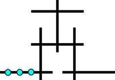
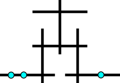
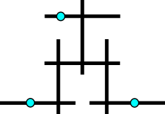
Figure -894: The type $IV^{*s}$ fibers. The sections, which intersect the components of the $IV^{*s}$ fiber represented by the blue nodes, are seen to intersect only the external, multiplicity one components. Because of the $S_{3}$ symmetry we write these as $IV^{*s(ijk)}$, $IV^{*s(ij|k)}$, and $IV^{*s(i|j|k)}$ respectively.

The starting point for the enhancements to the possible canonical exceptional singular fibers is the $I_{0}^{*ss(01|2)}:(2,2,1,1,1,0,0,0)$. Recall that one of the fiber components will split only if the condition $s_{5,1}^{2}-4s_{1,2}s_{8,0}=p^{2}$ is satisfied for some $p$. The discriminant at sixth order takes the form

$$\Delta=s_{7,0}^{2}s_{8,0}^{2}(s_{5,1}^{2}-4s_{1,2}s_{8,0})(s_{1,2}s_{7,0}^{2}-s_{3,1}s_{5,1}s_{7,0}+s_{3,1}^{2}s_{8,0})^{2})z^{6}+\mathcal{O}(z^{7})\,.$$ (6.1)

First let $z\mid{\mathfrak{s}}_{8}$ and the resulting fiber is of type $I_{1}^{s(0|2||1)}$. The discriminant at seventh order reads

$$\Delta=s_{5,1}^{3}s_{7,0}^{3}(s_{3,1}s_{5,1}-s_{1,2}s_{7,0})^{2}s_{9,0}^{2}z^{7}+\mathcal{O}(z^{8})\,.$$ (6.2)

Now let $z^{2}\mid{\mathfrak{s}}_{5}$ and the first exceptional singular fiber is found; it is of type $IV^{*(0|1|2)}$

$$IV^{*(0|1|2)}\,:\quad(2,2,1,2,1,0,1,0)\,.$$ (6.3)

This subbranch of the tree does not continue because the discriminant now takes the form $\Delta=s_{1,2}s_{7,0}s_{9,0}z^{8}+\mathcal{O}(z^{9}$) and the only possible enhancement that remains inside the lop-equivalence class, the vanishing of $s_{1,2}$, is a non-minimal enhancement.

Looking back at the $I_{0}^{*}$ starting point, the discriminant can instead be enhanced by letting the three-term polynomial vanish, through the canonical solution $s_{1,2}=s_{3,1}=0$. This gives an $I_{1}^{*s(01||2)}$ singular fiber. The discriminant at seventh order takes the form

$$\Delta=s_{2,2}^{2}s_{5,1}^{3}s_{7,0}^{5}s_{8,0}^{2}z^{7}+\mathcal{O}(z^{8})\,.$$ (6.4)

The discriminant is enhanced further by letting $s_{5,1}=0$. This gives the second exceptional singular fiber, that is a type $IV^{*(01|2)}$

$$IV^{*(01|2)}\,:\quad(3,2,2,2,1,0,0,0)\,.$$ (6.5)

Proceeding in this subbranch, the discriminant now reads

$$\Delta=s_{2,2}^{4}s_{7,0}^{4}s_{8,0}^{4}z^{8}+\mathcal{O}(z^{9})\,.$$ (6.6)

The only enhancement which is possible (as all the others are non-minimal enhancements) is $s_{2,2}=0$. The canonical excpetional singular fiber that arises from this enhancement is $III^{*(01|2)}$

$$III^{*(01|2)}\,:\quad(3,3,2,2,1,0,0,0)\,.$$ (6.7)

Every further enhancement in this subbranch is a non-minimal fibration.

6.2 Non-canonical Enhancements to Exceptional Singular Fibers

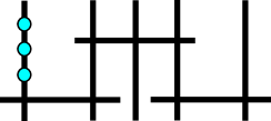
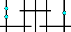
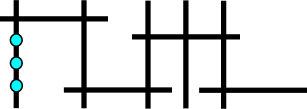
Figure -893: The type $III^{*}$ and $II^{*}$ fibers. Shown are the two type $III^{*(ijk)}$ and $III^{*(ij|k)}$ fibers where the sections are distributed over the two multiplicity one components, and the single type $II^{*(ijk)}$ fiber, which has all three sections intersecting the single multiplicity one component.

In this section the remaining exceptional fibers are obtained through non-canonical enhancements of the discriminant. The starting point is the singular $I_{3}^{ns(012)}$ given by the vanishing orders $(3,2,0,2,0,0,0,0)$. The discriminant contains $\Delta\supset(s_{6,0}^{2}-4s_{3,0}s_{8,0})$. Following appendix A it can be solved non-canonically to find a non-split $I_{0,nc}^{*ns(012)}$ associated to gauge group $G_{2}$

$$I_{0,nc}^{*ns(012)}:\quad\left\{\begin{array}[]{c}(3,2,0,2,0,0,0,0)\cr[-,-,\mu\sigma_{3}^{2},-,2\mu\sigma_{3}\sigma_{8},-,\mu\sigma_{8}^{2},-]\end{array}\right\}\,.$$ (6.8)

The next exceptional singular fiber is found through the following series of enhancements

$$I_{0,nc}^{*ns(012)} \overset{\{s_{1,3},s_{2,2},s_{5,2}=0\}}{\longrightarrow}\quad I_{1,nc}^{*ns(012)}\quad\overset{P=0}{\longrightarrow}\quad IV_{nc^{2}}^{*ns(012)}$$ (6.9)

$$P=(\sigma_{8}^{2}s_{3,1}-\sigma_{3}\sigma_{8}s_{6,1}+\sigma_{3}^{2}s_{8,1})\,.$$

Where the non-canonical solution to the three-term polynomial was applied to find a singular $IV_{nc^{2}}^{*ns(012)}$ with gauge group $F_{4}$

$$IV_{nc^{2}}^{*ns(012)}:\quad\left\{\begin{array}[]{c}(4,3,0,3,0,0,0,0)\cr[-,-,\mu\xi_{2}^{2}+\xi_{2}\xi_{5}z,-,2\mu\xi_{2}\xi_{3}+(\xi_{2}\xi_{4}+\xi_{3}\xi_{5})z,-,\mu\xi_{3}^{2}+\xi_{3}\xi_{4}z,-]\end{array}\right\}\,.$$ (6.10)

It was also necessary to specialize terms linear in $z$ in the expansion of the coefficients. From this singular fiber the remaining two fiber types can be reached through

$$IV_{nc^{2}}^{*ns(012)} \overset{s_{1,4}=0}{\longrightarrow}\quad III_{nc^{2}}^{*(012)}\overset{Q=0}{\longrightarrow}\quad II_{nc^{3}}^{*(012)}$$ (6.11)

$$Q=(s_{5,3}\xi_{2}-s_{2,3}\xi_{3})\,.$$

The singular fibers obtained this way are type $III_{nc^{2}}^{*(012)}$

$$III_{nc^{2}}^{*(012)}:\quad\left\{\begin{array}[]{c}(5,3,0,3,0,0,0,0)\cr[-,-,\mu\xi_{2}^{2}+\xi_{2}\xi_{5}z,-,2\mu\xi_{2}\xi_{3}+(\xi_{2}\xi_{4}+\xi_{3}\xi_{5})z,-,\mu\xi_{3}^{2}+\xi_{3}\xi_{4}z,-]\end{array}\right\}\,.$$ (6.12)

and the singular fiber type $II_{nc^{3}}^{*(012)}$

$$II_{nc^{3}}^{*(012)}:\quad\left\{\begin{array}[]{c}(5,3,0,3,0,0,0,0)\cr[-,\delta_{1}\delta_{3},\mu\delta_{3}^{2}+\delta_{3}\xi_{5}z,\delta_{1}\delta_{2},2\mu\delta_{2}\delta_{3}+(\delta_{3}\xi_{4}+\delta_{2}\xi_{5})z,-,\mu\delta_{2}^{2}+\delta_{2}\xi_{4}z,-]\end{array}\right\}\,.$$ (6.13)

Appendix A Solving Polynomial Equations over UFDs

In this appendix details are included of how to solve polynomial equations in the sections ${\mathfrak{s}}_{i}$ given that they belong to a unique factorization domain [60]. These solutions were repeatedly used in the algorithm to enhance the vanishing order of the discriminant. For convenience a part of this section will be a summary of the details given in the appendix A of [32], however there are polynomials specific to the case of two additional rational sections and the derivation of the solution for these is provided here. For more details on polynomial equations over UFDs that arise in the application of Tate’s algorithm the reader is referred to appendix B of [46].

In [32] solutions were obtained for a three-term polynomial of the form

$$s_{1}^{2}s_{2}-s_{1}s_{3}s_{4}+s_{3}^{2}s_{5}=0\,.$$ (A.1)

Four solutions were found, three of which involve setting pairs of terms to zero, which are what we refer to as canonical solutions of the polynomials, and one other solution which we refer to as the non-canonical solution. The canonical solutions were found to be the pairs

$$s_{1}=s_{3}=0$$ (A.2)

$$s_{1}=s_{5}=0$$

$$s_{2}=s_{3}=0\,.$$

The non-canonical solution is when

$$s_{1} =\sigma_{1}\sigma_{2}$$ (A.3)

$$s_{2} =\sigma_{3}\sigma_{4}$$

$$s_{3} =\sigma_{1}\sigma_{3}$$

$$s_{4} =\sigma_{2}\sigma_{4}+\sigma_{3}\sigma_{5}$$

$$s_{5} =\sigma_{2}\sigma_{5}\,,$$

where $\sigma_{2}$ and $\sigma_{3}$ are coprime over this UFD.

The non-canonical solution of a two-term polynomial was also needed

$$s_{1}s_{2}-s_{3}s_{4}=0:\quad\begin{cases}s_{1}=\sigma_{1}\sigma_{2}\\ s_{2}=\sigma_{3}\sigma_{4}\\ s_{3}=\sigma_{1}\sigma_{3}\\ s_{4}=\sigma_{2}\sigma_{4}\,.\end{cases}$$ (A.4)

With this solution $\sigma_{2}$ and $\sigma_{3}$ are coprime, and so are $\sigma_{1}$ and $\sigma_{4}$.

A.1 Two Term Polynomial

We now look at the polynomial

$$P=s_{1}^{2}-4s_{2}s_{3}\,.$$ (A.5)

Setting $P=0$ imposes the following conditions:

• There is an equality between the irreducible components of $s_{1}^{2}$ and the product of the irreducibles of $s_{2}$ and $s_{3}.$

• Write $\mu$ for the irreducible components common to all the three terms.

• Write $\sigma_{1}$ for the irreducible components common to $s_{1}$ and $s_{2}$.

• Write $\sigma_{2}$ for the irreducible components common to $s_{1}$ and $s_{3}$.

Note that no conclusion is drawn about irreducibles shared only by $s_{2}$ and $s_{3}$. Then the most general solution takes the form

$$s_{1}^{2}-4s_{2}s_{3}=0:\quad\begin{cases}s_{1}=2\mu\sigma_{1}\sigma_{2}\\ s_{2}=\mu\sigma_{1}^{2}\\ s_{3}=\mu\sigma_{2}^{2}\,.\end{cases}$$ (A.6)

Since $\mu$ is the greatest common divisor of $s_{2}$ and $s_{3}$ we have that $\sigma_{1}$ and $\sigma_{2}$ are coprime.

A.2 Perfect Square Polynomial

The first perfect square polynomial is given by

$$s_{1}^{2}-4s_{2}s_{3}=p^{2}\,.$$ (A.7)

This can be reformulated as

$$\left(s_{1}+p\right)\left(s_{1}-p\right)=4s_{2}s_{3}\,,$$ (A.8)

which can be solved in general by applying the solution of the two-term polynomial (A.4). In this case, it reads

$$s_{1}-p =2\sigma_{1}\sigma_{2}$$ (A.9)

$$s_{1}+p =2\sigma_{3}\sigma_{4}$$

$$s_{2} =\sigma_{1}\sigma_{3}$$

$$s_{3} =\sigma_{2}\sigma_{4}\,.$$

From the first two of these equations, one finds the generic form of $s_{1}$

$$s_{1}=\sigma_{1}\sigma_{2}+\sigma_{3}\sigma_{4}\,.$$ (A.10)

So the general solution to the perfect square condition is

$$s_{1}^{2}-4s_{2}s_{3}=p^{2}:\quad\begin{cases}s_{1}=\sigma_{1}\sigma_{2}+\sigma_{3}\sigma_{4}\\ s_{2}=\sigma_{1}\sigma_{3}\\ s_{3}=\sigma_{2}\sigma_{4}\,.\end{cases}$$ (A.11)

It follows from the solution of (A.4) that $\sigma_{2}$ and $\sigma_{3}$ are coprime, as are $\sigma_{1}$ and $\sigma_{4}$.

A.3 Three Term Polynomial

The three-term polynomial

$$P=s_{1}^{2}s_{2}s_{3}-s_{1}s_{4}s_{5}+s_{5}^{2}s_{6}\,,$$ (A.12)

appears in the algorithm. By imposing $P=0$ it is seen that $s_{1}\mid s_{5}^{2}s_{6}$, since it divides the other two terms in the equation. In the same way $s_{5}\mid s_{1}^{2}s_{2}s_{3}$. Decompose $s_{5}=\sigma_{1}\sigma_{2}$ and $s_{1}=\sigma_{1}\sigma_{3}$, where $\sigma_{1}=(s_{1},s_{5})$ is the greatest common divisor of the two terms, so that $\sigma_{2}$ and $\sigma_{3}$ have no common irreducibles. Then the equation of the polynomial becomes

$$\sigma_{1}^{2}(s_{6}\sigma_{2}^{2}-s_{4}\sigma_{2}\sigma_{3}+s_{2}s_{3}\sigma_{3}^{2})=0\,.$$ (A.13)

Applying the same reasoning it is now seen that $\sigma_{3}\mid s_{6}\sigma_{2}$, but since $\sigma_{2}$ and $\sigma_{3}$ have no common irreducibles one can conclude that $\sigma_{3}\mid s_{6}$. In the same way it can be deduced that $\sigma_{2}\mid s_{2}s_{3}$. This can be expressed as

$$s_{6}=\sigma_{4}\sigma_{3},\qquad s_{2}s_{3}=\kappa\sigma_{2}\,,$$ (A.14)

where $\kappa$ is some constant of proportionality. The two-term solution (A.4) can be applied to the second of these equations to obtain

$$s_{2}=\sigma_{5}\sigma_{6},\quad s_{3}=\sigma_{7}\sigma_{8},\quad\kappa=\sigma_{5}\sigma_{7},\quad\sigma_{2}=\sigma_{6}\sigma_{8}\,.$$ (A.15)

Then the initial polynomial reduces to

$$\sigma_{1}^{2}\sigma_{3}\sigma_{6}\sigma_{8}(\sigma_{3}\sigma_{5}\sigma_{7}+\sigma_{4}\sigma_{6}\sigma_{8}-s_{4})=0\,,$$ (A.16)

from which can be solved for $s_{4}$. Then there is a non-canonical solution

$$s_{1}^{2}s_{2}s_{3}-s_{1}s_{4}s_{5}+s_{5}^{2}s_{6}=0:\quad\begin{cases}s_{1}=\sigma_{1}\sigma_{3}\\ s_{2}=\sigma_{5}\sigma_{6}\\ s_{3}=\sigma_{7}\sigma_{8}\\ s_{4}=\sigma_{3}\sigma_{5}\sigma_{7}+\sigma_{4}\sigma_{6}\sigma_{8}\\ s_{5}=\sigma_{1}\sigma_{6}\sigma_{8}\\ s_{6}=\sigma_{3}\sigma_{4}\,,\end{cases}$$ (A.17)

where the pairs $(\sigma_{5},\sigma_{8})$, $(\sigma_{6},\sigma_{7})$, and $(\sigma_{3},\sigma_{6}\sigma_{8})$ are all coprime. There are also four different canonical solutions

$$\sigma_{1}=0: \quad s_{1}=s_{5}=0$$ (A.18)

$$\sigma_{3}=0: \quad s_{1}=s_{6}=0$$

$$\sigma_{6}=0: \quad s_{2}=s_{5}=0$$

$$\sigma_{8}=0: \quad s_{3}=s_{5}=0\,.$$

Appendix B Matter Loci of $SU(5)$ Models

In this appendix we list the matter loci of the $I_{5}$ fibers whose $U(1)$ charges are studied in section 5.

$$\sigma_{3}^{2}s_{1,2}-\sigma_{2}\sigma_{3}s_{2,2}+\sigma_{2}^{2}s_{3,2}$$ (B.1)

$$\sigma_{4}^{2}s_{1,2}-\sigma_{4}\sigma_{5}s_{2,2}+\sigma_{5}^{2}s_{3,2}$$ (B.2)

$$\sigma_{1}(\sigma_{3}^{2}s_{5,1}-\sigma_{2}\sigma_{3}s_{6,1}+\sigma_{2}^{2}s_{7,1})-(\sigma_{2}\sigma_{4}-\sigma_{3}\sigma_{5})(\sigma_{2}s_{9,1}-\sigma_{3}s_{8,1})$$ (B.3)

$$\sigma_{3}^{2}\sigma_{4}(\sigma_{4}s_{3,1}-\sigma_{1}s_{7,0})+\sigma_{2}^{2}(\sigma_{4}^{2}s_{1,3}-\sigma_{1}\sigma_{4}s_{5,2}+\sigma_{1}^{2}s_{8,1})-\sigma_{2}\sigma_{3}(\sigma_{4}^{2}s_{2,2}-\sigma_{1}\sigma_{4}s_{6,1}+\sigma_{1}^{2}s_{9,0})$$ (B.4)

$$\sigma_{3}^{2}\sigma_{4}(\sigma_{4}s_{1,2}-\sigma_{1}s_{5,1})+\sigma_{2}^{2}\sigma_{4}(\sigma_{4}s_{3,2}-\sigma_{1}s_{7,1})-\sigma_{2}\sigma_{3}(\sigma_{4}^{2}s_{2,2}-\sigma_{1}\sigma_{4}s_{6,1}+\sigma_{1}^{2}s_{9,0})$$ (B.5)

$$\sigma_{1}^{2}\sigma_{2}^{2}s_{1,3}-\sigma_{1}\sigma_{2}s_{2,2}s_{5,1}+s_{3,1}s_{5,1}^{2}$$ (B.6)

$$-\sigma_{1}\sigma_{3}^{2}\sigma_{4}s_{5,1}-\sigma_{2}\sigma_{3}(\sigma_{4}^{2}s_{3,1}-\sigma_{1}\sigma_{4}s_{6,1}+\sigma_{1}^{2}s_{8,1})+\sigma_{1}\sigma_{2}^{2}(-\sigma_{4}s_{7,1}+\sigma_{1}s_{9,1})$$ (B.7)

$$\sigma_{1}^{2}\sigma_{3}(\sigma_{3}^{2}s_{1,4}-\sigma_{2}\sigma_{3}s_{2,3}+\sigma_{2}^{2}s_{3,2})+\sigma_{1}(\sigma_{2}\sigma_{4}-\sigma_{3}\sigma_{5})(\sigma_{3}^{2}s_{5,2}-\sigma_{2}\sigma_{3}s_{6,1}+\sigma_{2}^{2}s_{7,0})+\sigma_{3}(\sigma_{2}\sigma_{4}-\sigma_{3}\sigma_{5})^{2}s_{8,0}$$ (B.8)

$$\sigma_{1}(\sigma_{2}^{2}s_{3,1}-\sigma_{2}\sigma_{3}s_{6,1}+\sigma_{3}^{2}s_{8,1})-(\sigma_{2}\sigma_{4}-\sigma_{3}\sigma_{5})(\sigma_{2}s_{7,1}-\sigma_{3}s_{9,1})$$ (B.9)

$$(\sigma_{2}\sigma_{4}-\sigma_{3}\sigma_{5})^{2}s_{1,4}+\sigma_{2}\sigma_{5}s_{2,2}^{2}-(\sigma_{2}\sigma_{4}-\sigma_{3}\sigma_{5})s_{2,2}s_{5,2}+\sigma_{3}\sigma_{4}s_{5,2}^{2}$$ (B.10)

$$(\sigma_{2}\sigma_{4}-\sigma_{3}\sigma_{5})s_{1,5}-\sigma_{1}(\sigma_{2}\sigma_{4}-\sigma_{3}\sigma_{5})(\sigma_{2}s_{5,3}-\sigma_{3}s_{2,3})+\sigma_{1}^{2}(\sigma_{3}^{2}s_{3,1}-\sigma_{2}\sigma_{3}s_{6,1}+\sigma_{2}^{2}s_{8,1})$$ (B.11)

$$(\xi_{3}\sigma_{2}-\xi_{2}\sigma_{3})(\xi_{2}^{2}s_{1,3}-\xi_{2}\xi_{3}s_{2,3}+\xi_{3}^{2}s_{3,3})+(\xi_{2}\xi_{4}-\xi_{3}\xi_{5})(\xi_{2}^{2}s_{5,1}-\xi_{2}\xi_{3}s_{6,1}+\xi_{3}^{2}s_{7,1})$$ (B.12)

$$\xi_{3}\xi_{4}\sigma_{1}^{2}-\sigma_{1}\sigma_{4}s_{5,1}+\sigma_{4}^{2}s_{1,2}$$ (B.13)

$$\xi_{2}^{2}(\sigma_{1}s_{5,1}-\sigma_{4}s_{1,2})+\xi_{2}\xi_{3}(\sigma_{4}s_{2,2}-\sigma_{1}s_{6,1})+\xi_{3}^{2}(\sigma_{1}s_{7,1}-\sigma_{4}s_{3,2})$$ (B.14)

$$\xi_{2}^{2}\xi_{4}s_{5,1}+\xi_{2}\xi_{3}(\sigma_{4}s_{8,1}-\xi_{4}s_{6,1})+\xi_{3}^{2}(\xi_{4}s_{7,1}-\sigma_{4}s_{9,1})$$ (B.15)

$$\xi_{2}(-\xi_{2}\sigma_{2}s_{2,2}+\xi_{2}\sigma_{3}s_{3,2}+\xi_{3}\sigma_{2}s_{6,1}-\xi_{3}\sigma_{3}s_{7,1})-\xi_{3}^{2}\sigma_{2}s_{9,0}$$ (B.16)

$$\xi_{2}^{3}(\sigma_{3}s_{1,3}-\xi_{4}s_{2,2})+\xi_{2}^{2}\xi_{3}(\xi_{5}s_{2,2}-\sigma_{3}s_{5,2}+\xi_{4}s_{6,1})+\xi_{3}^{3}\xi_{5}s_{9,0}-\xi_{2}\xi_{3}^{2}(\xi_{5}s_{6,1}-\sigma_{3}s_{8,1}+\xi_{4}s_{9,0})$$ (B.17)

$$\xi_{1}\xi_{2}^{2}\xi_{4}s_{3,1}+\xi_{2}\xi_{3}(\xi_{4}^{2}\sigma_{4}-\xi_{1}\xi_{4}s_{6,1}+\xi_{1}^{2}\sigma_{2}s_{7,1})+\xi_{1}\xi_{3}^{2}(\xi_{4}s_{8,1}-\xi_{1}\sigma_{2}s_{9,1})$$ (B.18)

$$(\xi_{1}\xi_{2}\sigma_{3}-\sigma_{2}\sigma_{4})^{2}s_{3,1}+\xi_{3}(\xi_{1}\xi_{2}\sigma_{3}-\sigma_{2}\sigma_{4})(\xi_{1}\sigma_{2}s_{2,2}-\xi_{1}\sigma_{3}s_{6,1}+\xi_{4}\sigma_{3}\sigma_{4})+\xi_{1}^{2}\xi_{3}^{2}(\sigma_{2}^{2}s_{1,3}-\sigma_{2}\sigma_{3}s_{5,2}+\sigma_{3}^{2}s_{8,1})$$ (B.19)

$$\xi_{4}\xi_{6}^{3} \xi_{8}^{3}\sigma_{4}-\xi_{3}\xi_{6}^{2}\xi_{8}^{2}(\xi_{5}\xi_{7}\sigma_{4}-s_{1,2}+\xi_{4}s_{6,1})$$ (B.20)

$$+\xi_{3}^{2}\xi_{6}\xi_{8}(\xi_{4}\xi_{7}\xi_{8}\sigma_{3}-\xi_{5}\xi_{6}s_{5,2}+\xi_{5}\xi_{7}s_{6,1}+\xi_{4}\xi_{5}\xi_{6}s_{9,1})-\xi_{3}^{2}\xi_{5}(\xi_{7}^{2}\xi_{8}\sigma_{3}-\xi_{5}\xi_{6}^{2}s_{8,2}+\xi_{5}\xi_{6}\xi_{7}s_{9,1})$$

$$\xi_{3}^{3}\xi_{4}\xi_{7}\sigma_{3}^{3}-\xi_{5}\xi_{6}^{3}\xi_{8}\sigma_{3}\sigma_{4}^{2} +\xi_{3}^{2}\xi_{6}(\xi_{5}^{2}\xi_{6}^{2}s_{3,2}+\sigma_{3}^{2}(s_{1,2}-\xi_{4}s_{6,1})-\xi_{5}\sigma_{3}(\xi_{7}\sigma_{3}\sigma_{4}+\xi_{6}s_{2,2}-\xi_{4}\xi_{6}s_{7,1}))$$ (B.21)

$$+\xi_{3}\xi_{6}^{2}\sigma_{4}(\xi_{4}\xi_{8}\sigma_{3}^{2}+\xi_{5}(\sigma_{3}s_{6,1}-\xi_{5}\xi_{6}s_{7,1}))$$

$$\delta_{1}(\xi_{2}^{2}s_{1,2}-\xi_{2}\xi_{3}s_{2,2}+\xi_{3}^{2}s_{3,2})-\delta_{4}(\xi_{2}^{2}s_{5,1}-\xi_{2}\xi_{3}s_{6,1}+\xi_{3}^{2}s_{7,1})$$ (B.22)

$$\xi_{2}^{2}(\sigma_{1}s_{5,1}-\delta_{1}\sigma_{3}s_{8,1})+\xi_{3}^{2}(\sigma_{2}s_{7,1}-\delta_{1}\delta_{2}s_{9,1})+\xi_{2}\xi_{3}(-\sigma_{1}s_{6,1}+\delta_{1}\delta_{2}s_{8,1}+\delta_{1}\delta_{3}s_{9,1})$$ (B.23)

$$\delta_{2}\delta_{4}^{2}\sigma_{1}(\delta_{2}\xi_{3}-\delta_{3}\xi_{2})+\delta_{1}^{2}(\delta_{2}^{2}s_{1,2}-\delta_{2}\delta_{3}s_{2,2}+\delta_{3}^{2}s_{3,2})-\delta_{1}\delta_{4}(\delta_{2}^{2}s_{5,1}-\delta_{2}\delta_{3}s_{6,1}+\delta_{3}^{2}s_{7,1})$$ (B.24)

Appendix C Resolution of Generic Singular Fibers

In section 2 a table (table 4) of canonical forms for many of the different fiber types as originally denoted by Kodaira was presented. In this section is is shown by explicitly constructing the resolution that each of the forms is the stated fiber. Given the set of resolutions and the canonical vanishing orders, the resolved geometry is uniquely determined and the form of the resolved geometry will not be written explicitly. For the Cartan divisors the equations are given after the resolution process and they will intersect according to the fiber type of the singularity under consideration.

C.1 $I_{2k+1}^{s(0|^{n}1|^{m}2)}$ ($n+m\leq k$)

The generic form for the singular $I_{2k+1}^{s(0|^{n}1|^{m}2)}$ is $(2k+1-(n+m),k-n,m,k+1-m,0,0,n,0)$, provided that $(m+n\leq k)$. The resolution process involves several steps. First perform the following blow ups

$$(x,y,z;\zeta_{1}),\quad(x,y,\zeta_{i};\zeta_{i+1}) 1\leq i<\text{min}\{k-n,k+1-m\}\,.$$ (C.1)

If $n\neq 0$ then the following small resolutions can be applied

$$(x,z;\xi_{1}),\quad(x,\xi_{i};\xi_{i+1}) 1\leq i<n\,.$$ (C.2)

Similarly if $m\neq 0$ the small resolutions,

$$(y,z;\delta_{1}),\quad(y,\delta_{j};\delta_{j+1}) 1\leq j<m\,,$$ (C.3)

are possible. If both $n\neq 0$ and $m\neq 0$ we need to use both sets of resolutions are applied. The next step depends on the sign of the quantity $m-n-1$. We call $\zeta_{max}$ the last exceptional divisor introduced in the initial blow ups, and from now on the index will be used as $\text{max}=\text{min}\{k-n,k+1-m\}$ If it is positive then the resolutions,

$$(y,\zeta_{max};\chi_{1}),\quad(y,\chi_{r};\chi_{r+1})\qquad 1\leq r<m-n-1\,,$$ (C.4)

are used. Whereas if negative then the resolutions are

$$(x,\zeta_{max};\Omega_{1}),\quad(x,\Omega_{r};\Omega_{r+1})\qquad 1\leq r<-(m-n-1)\,.$$ (C.5)

If the term is exactly zero then we do neither set. Finally the process can be completed with the resolutions

$$(y,\zeta_{s};\psi_{s}) 1\leq s<\text{max}\,.$$ (C.6)

The Cartan divisors are listed, assuming that $n-m-1>0$,

Exceptional Divisor	Fiber Equation
$z$	$l_{1}l_{2}ws_{6,0}+l_{2}s_{9,0}\zeta_{1}\delta_{1}+l_{1}s_{7,0}\zeta_{1}\xi_{1}$
$\zeta_{i<max}$	$s_{6,0}x$
$\zeta_{max}$	$xs_{6,0}+s_{5,k+1-m}\zeta_{max-1}$
$\delta_{j<m}$	$l_{2}s_{6,0}+s_{7,0}\zeta_{1}$
$\delta_{m}$	$l_{2}ys_{6,0}+ys_{7,0}\zeta_{1}\psi_{1}+s_{3,m}\zeta_{1}^{m}\delta_{m-1}\psi_{1}^{m-1}$
$\xi_{i<n}$	$l_{1}s_{6,0}+s_{9,0}\zeta_{1}$
$\xi_{n}$	$l_{1}xs_{6,0}+\zeta_{1}(xs_{9,0}+s_{8,0}\zeta_{1}^{n-1}\xi_{n-1})$
$\chi_{r<m-n-1}$	$xs_{6,0}+s_{5,k+1-m}\zeta_{max-1}$
$\chi_{m-n-1}$	$\begin{aligned} &y(xs_{6,0}+s_{5,k+1-m}\zeta_{max-1}\psi_{max-1})+\\ +\zeta_{\max-1}^{m-n}\psi_{max-1}^{m-n-1}&(xs_{2,k-n}+s_{1,2k+1-n-m}\zeta_{max-1}\psi_{max-1})\chi_{m-n-2}\end{aligned}$
$\psi_{s<max}$	$s_{6,0}y$

Then the ordered set $(z,\xi_{1},\cdots,\xi_{n},\zeta_{1},\cdots,\zeta_{max},\chi_{1},\cdots,\chi_{m-n-1},\psi_{max},\cdots,\psi_{1}\delta_{m},\cdots,\delta_{1})$ gives an $I_{2k+1}^{s(0|^{n}1|^{m}2)}$ fiber, where the divisors are listed in the canonical ordering for the Dynkin diagram. One gets the analogous result when $n-m-1<0$.

C.2 $I_{2k+1}^{s(0|^{n}1|^{m}2)}$ ($k<n+m\leq\left\lfloor{\frac{2}{3}(2k+1)}\right\rfloor$)

The generic form for the singular fibers of type $I_{2k+1}^{s(0|^{n}1|^{m}2)}$ with section separation of the form $m+n\leq\left\lfloor{\frac{2}{3}(2k+1)}\right\rfloor$ is given by $(2k+1-(m+n),m,m,n,0,0,n,0)$, where it is assumed that $m\geq n$. In order to resolve the geometry the following set of resolutions is used

$$(x,z;\xi_{1}),\qquad(x,\xi_{i};\xi_{i+1}) 1\leq i<n$$ (C.7)

$$(y,z;\delta_{1}),\qquad(y,\delta_{j};\delta_{j+1}) 1\leq j<m$$

$$(x,\delta_{r};\chi_{r}) 1\leq r\leq m$$

$$(x,\chi_{m};\psi_{1}),\qquad(x,\psi_{s};\psi_{s+1}) 1\leq s<2k-2m-n\,.$$

Notice that the first three set of resolutions (together with $z$) produce $2m+n+1$ Cartan divisors. The fourth set of resolutions is only necessary if $2k-2m-n>0$. Then the Cartan divisors in the most general case are

Exceptional Divisor	Fiber Equation
$z$	$l_{1}l_{2}ws_{6,0}+l_{2}s_{9,0}\delta_{1}+l_{1}s_{7,0}\xi_{1}$
$\delta_{1}$	$l_{2}s_{6,0}+s_{7,0}\xi_{1}\xi_{2}^{2}\cdots\xi_{n}^{n}\chi_{1}$
$\delta_{j<m}$	$l_{2}s_{6,0}+s_{7,0}\chi_{j-1}\chi_{j}$
$\delta_{m}$	$l_{2}(ys_{6,0}+s_{2,m}\delta_{m-1}\chi_{m-1})+\chi_{m-1}(ys_{7,0}+s_{3,m}\delta_{m-1}\chi_{m-1})\chi_{m}$
$\xi_{i<n}$	$l_{1}s_{6,0}+s_{9,0}\delta_{1}$
$\xi_{n}$	$l_{1}xs_{6,0}+xs_{9,0}\delta_{1}\chi_{1}+l_{1}s_{5,n}\delta_{1}^{n}\xi_{n-1}\chi_{1}^{n-1}+s_{8,n}\delta_{1}^{n+1}\xi_{n-1}\chi_{1}^{n}$
$\chi_{r<m}$	$xs_{6,0}$
$\chi_{m}$	$ys_{6,0}+s_{2,m}\chi_{m-1}$
$\psi_{s<2k-2m-n}$	$ys_{6,0}+s_{2,m}\chi_{m-1}$
$\psi_{2k-2m-n}$	$xys_{6,0}+xs_{2,m}\chi_{m-1}+s_{1,2k+1-m-n}\psi_{2k-2m-n-1}\chi_{m-1}^{n-1}$

The ordered set $(z,\xi_{1},\cdots,\xi_{n},\chi_{1},\cdots,\chi_{m-1},\psi_{2k-2m-n},\cdots,\psi_{1},\chi_{m},\delta_{m},\cdots,\delta_{1})$ gives an $I_{2k+1}^{s(0|^{n}1|^{m}2)}$ singular fiber.

C.3 $I_{2k}^{s(0|^{n}1|^{m}2)}$ ($n+m\leq k,\quad m<k$)

The generic form for the singular fiber of type $I_{2k}^{s(0|^{n}1|^{m}2)}$, where $m+n\leq k$, is given by $(2k-(n+m),k-n,m,k-m,0,0,n,0)$. The analysis follows closely that carried out for $I_{2k+1}^{s(0|^{n}1|^{m}2)}$ where more details can be found. In order to resolve the geometry perform the resolutions

$$(x,y,z;\zeta_{1}),\quad(x,y,\zeta_{i};\zeta_{i+1}) 1\leq i<\text{min}\{k-n,k-m\}$$ (C.8)

$$(x,z;\xi_{1}),\qquad(x,\xi_{i};\xi_{i+1}) 1\leq i<n$$

$$(y,z;\delta_{1}),\qquad(y,\delta_{j};\delta_{j+1}) 1\leq j<m\,.$$

Then the sign of the quantity $m-n$ and then use the according set of small resolutions, where the index in $\zeta_{max}$ again means the last exceptional divisor introduced in the blow ups, that is, $\text{max}=\text{min}\{k-n,k-m\}$

$$(y,\zeta_{max};\chi_{1}),\quad(y,\chi_{r};\chi_{r+1}) 1\leq r<m-n$$ (C.9)

$$(x,\zeta_{max};\Omega_{1}),\quad(x,\Omega_{r};\Omega_{r+1}) 1\leq r<-(m-n)\,.$$

Finally the resolution process is completed with

$$(y,\zeta_{s};\psi_{s}) 1\leq s<\text{max}\,.$$ (C.10)

The Cartan divisors are, assuming $m-n>0$,

Exceptional Divisor	Fiber Equation
$z$	$l_{1}l_{2}ws_{6,0}+l_{2}s_{9,0}\zeta_{1}\delta_{1}+l_{1}s_{7,0}\zeta_{1}\xi_{1}$
$\zeta_{i<max}$	$s_{6,0}x$
$\zeta_{max}$	$xs_{6,0}+s_{5,k-m}\zeta_{max-1}$
$\delta_{j<m}$	$l_{2}s_{6,0}+s_{7,0}\zeta_{1}$
$\delta_{m}$	$l_{2}ys_{6,0}+ys_{7,0}\zeta_{1}\psi_{1}+s_{3,0}\zeta_{1}^{m}\delta_{m-1}\psi_{1}^{m-1}$
$\xi_{i<n}$	$l_{1}s_{6,0}+s_{9,0}\zeta_{1}$
$\xi_{n}$	$l_{1}xs_{6,0}+\zeta_{1}(xs_{9,0}+s_{8,n}\zeta_{1}^{n-1}\xi_{n-1})$
$\chi_{r<m-n}$	$xs_{6,0}+s_{5,k-m}\zeta_{max-1}$
$\chi_{m-n}$	$\begin{aligned} &y(xs_{6,0}+s_{5,k-m}\zeta_{max-1}\psi_{max-1})+\\ +\zeta_{\max-1}^{m-n+1}\psi_{max-1}^{m-n}(x&s_{2,k-n}+s_{1,2k-m-n}\zeta_{max-1}\psi_{max-1})\chi_{m-n-1}\end{aligned}$
$\psi_{s<max}$	$s_{6,0}y$

Then the ordered set $(z,\xi_{1},\cdots,\xi_{n},\zeta_{1},\cdots,\zeta_{max},\chi_{1},\cdots,\chi_{m-n-1},\psi_{max},\cdots,\psi_{1},\delta_{m},\cdots,\delta_{1})$ gives an $I_{2k+1}^{s(0|^{n}1|^{m}2)}$, and again analogously for $m-n<0$. Notice that if $m=k$ and $n=0$ the vanishing orders $(k,k,k,0,0,0,0,0)$ specify the singular fibers $I_{2k}^{ns(01|^{n}2)}$ as listed in table 4. The $k$ small resolutions that resolve the singularity are

$$(y,z;\delta_{1}),\qquad(y,\delta_{j};\delta_{j+1})\qquad 1\leq j<k\,.$$ (C.11)

The resolved geometry has $k+1$ Cartan divisors, $k-1$ of which will split if $s_{6,0}^{2}-4s_{5,0}s_{7,0}$ is a perfect, non-zero, square.

C.4 $I_{2k}^{s(0|^{n}1|^{m}2)}$ ($n+m\leq\left\lfloor{\frac{4}{3}k}\right\rfloor$)

The generic form for the singular fibers of type $I_{2k}^{s(0|^{n}1|^{m}2)}$ with section separation such that $m+n\leq\left\lfloor{\frac{4}{3}k}\right\rfloor$ is given by $(2k-(m+n),m,m,n,0,0,n,0)$, where it is assumed that $m\geq n$. In order to resolve the geometry the following set of resolutions is used

$$(x,z;\xi_{1}),\qquad(x,\xi_{i};\xi_{i+1}) 1\leq i<n$$ (C.12)

$$(y,z;\delta_{1}),\qquad(y,\delta_{j};\delta_{j+1}) 1\leq j<m$$

$$(x,\delta_{r};\chi_{r}) 1\leq r\leq m$$

$$(x,\chi_{m};\psi_{1}),\qquad(x,\psi_{s};\psi_{s+1}) 1\leq s<2k-2m-n-1\,.$$

Notice that the first three sets of resolutions produce $2m+n+1$ Cartan divisors. The fourth set of resolutions is then necessary if $2k-2m-n-1\neq 0$. The Cartan divisors in the most general case are

Exceptional Divisor	Fiber Equation
$z$	$l_{1}l_{2}ws_{6,0}+l_{2}s_{9,0}\delta_{1}+l_{1}s_{7,0}\xi_{1}$
$\delta_{1}$	$l_{2}s_{6,0}+s_{7,0}\xi_{1}\xi_{2}^{2}\cdots\xi_{n}^{n}\chi_{1}$
$\delta_{j<m}$	$l_{2}s_{6,0}+s_{7,0}\chi_{j-1}\chi_{j}$
$\delta_{m}$	$l_{2}(ys_{6,0}+s_{2,m}\delta_{m-1}\chi_{m-1})+\chi_{m-1}(ys_{7,0}+s_{3,m}\delta_{m-1}\chi_{m-1})\chi_{m}$
$\xi_{i<n}$	$l_{1}s_{6,0}+s_{9,0}\delta_{1}$
$\xi_{n}$	$l_{1}xs_{6,0}+xs_{9,0}\delta_{1}\chi_{1}+l_{1}s_{5,n}\delta_{1}^{n}\xi_{n-1}\chi_{1}^{n-1}+s_{8,n}\delta_{1}^{n+1}\xi_{n-1}\chi_{1}^{n}$
$\chi_{r<m}$	$xs_{6,0}$
$\chi_{m}$	$ys_{6,0}+s_{2,m}\chi_{m-1}$
$\psi_{s<2k-2m-n-1}$	$ys_{6,0}+s_{2,m}\chi_{m-1}$
$\psi_{2k-2m-n-1}$	$xys_{6,0}+xs_{2,m}\chi_{m-1}+s_{1,2k-m-n}\psi_{2k-2m-n-2}\chi_{m-1}^{n-2}$

The ordered set $(z,\xi_{1},\cdots,\xi_{n},\chi_{1},\cdots,\chi_{m-1},\psi_{2k-2m-n-1},\cdots,\psi_{1},\chi_{m},\delta_{m},\cdots,\delta_{1})$ gives an $I_{2k}^{s(0|^{n}1|^{m}2)}$ type singular fiber.

C.5 $I_{2k+1}^{ns(012)}$

The generic form for $I_{2k+1}^{ns(012)}$ is $(2k+1,k+1,0,k+1,0,0,0,0)$. The geometry is singular at $x=y=z=0$ and it can be resolved by performing a blow up $(x,y,z;\zeta_{1})$. This process can be repeated $k$ times, with the $i^{\text{th}}$ resolution being $(x,y,\zeta_{i-1};\zeta_{i})$. The Cartan divisors are then

Exceptional Divisor	Fiber Equation
$z$	$l_{1}wx(l_{1}xs_{3,0}+l_{2}ys_{6,0})+l_{2}^{2}wy^{2}s_{8,0}+xy(l_{1}xs_{7,0}+l_{2}ys_{9,0})\zeta_{1}$
$\zeta_{i\leq k}$	$x^{2}s_{3,0}+xys_{6,0}+y^{2}s_{8,0}$

It is easily seen by considering the projective relations introduced by the resolutions the ordered set $(z,\zeta_{1},\cdots,\zeta_{k})$ of Cartan divisors intersects in an $I_{2k+1}^{ns(012)}$. Notice that if $s_{6,0}^{2}-4s_{3,0}s_{8,0}$ is a perfect square, each of the fiber components along $\{\zeta_{i}=0\}$ splits into two, thus giving the split version $I_{2k+1}^{s(012)}$.

C.6 $I_{2k}^{ns(012)}$

The generic form for $I_{2k}^{ns(012)}$ is $(2k,k,0,k,0,0,0,0)$. The singular geometry can be blown up $k$ times with the $i^{\text{th}}$ resolution being $(x,y,\zeta_{i-1};\zeta_{i})$. The Cartan divisors are

Exceptional Divisor	Fiber Equation
$z$	$l_{1}wx(l_{1}xs_{3,0}+l_{2}ys_{6,0})+l_{2}^{2}wy^{2}s_{8,0}+xy(l_{1}xs_{7,0}+l_{2}ys_{9,0})\zeta_{1}$
$\zeta_{i<k}$	$x^{2}s_{3,0}+xys_{6,0}+y^{2}s_{8,0}$
$\zeta_{k}$	$x^{2}s_{3,0}+xys_{6,0}+y^{2}s_{8,0}+\zeta_{k-1}xs_{2,k}+\zeta_{k-1}ys_{5,k}s_{1,2k}\zeta_{k-1}^{2}$

The ordered set of $(k+1)$ Cartan divisors $(z,\zeta_{1},\cdots,\zeta_{k})$ gives an $I_{2k}^{ns(012)}$. If, in addition, $s_{6,0}^{2}-4s_{3,0}s_{8,0}$ is a perfect square the $(k-1)$ Cartan divisors along $\zeta_{i}$ split into two, giving an $I_{2k}^{s(012)}$ fiber.

C.7 $I_{2k+1}^{*s(0|1||2)}$

The generic forms for the singular fibers of type $I_{2k+1}^{*s(0|1||2)}$ are characterized by the vanishing orders $(k+2,k+2,k+1,1,1,0,1,0)$. In order to resolve the geometry perform the resolutions

$$(x,y,z;\zeta_{1}),\quad(z,\zeta_{1};\zeta_{2}), (x,z;\zeta_{3}),\quad(y,z;\zeta_{4}),\quad(y,\zeta_{2};\delta_{1})$$ (C.13)

$$(y,\delta_{i};\delta_{i+1})\qquad 1\leq i\leq 2k\,.$$

The Cartan divisors are

Exceptional Divisor	Fiber Equation
$z$	$l_{1}s_{7,0}\zeta_{3}+l_{2}s_{9,0}\zeta_{4}$
$\zeta_{1}$	$ys_{5,1}$
$\zeta_{2}$	$s_{5,1}z\zeta_{4}+x\zeta_{1}(xs_{7,0}\zeta_{3}+s_{9,0}\zeta_{4}\delta_{1})$
$\zeta_{3}$	$xs_{9,0}+z(l_{1}s_{5,1}+s_{8,1}\zeta_{2})$
$\zeta_{4}$	$ys_{7,0}$
$\delta_{i\leq 2k}$	$s_{7,0}\zeta_{1}+s_{5,1}\zeta_{4}$
$\delta_{2k+1}$	$y(s_{7,0}\zeta_{1}+s_{5,1}\zeta_{4})+\zeta_{1}^{k}\zeta_{4}^{k}(s_{3,k+1}\zeta_{1}+s_{1,k+2}\zeta_{4})\delta_{2k}$

The ordered set of divisors $(z,\zeta_{3},\zeta_{2},\delta_{1},\cdots,\delta_{2k+1},\zeta_{1},\zeta_{4})$ specifies an $I_{2k+1}^{*s(0|1||2)}$ fiber in the canonical ordering.

C.8 $I_{2k}^{*s(0|1||2)}$

The generic forms for the singular fibers of type $I_{2k+1}^{*s(0|1||2)}$ are given by the vanishing orders $(k+2,k+1,k+1,1,1,0,1,0)$. In order to resolve the geometry the following resolutions are used

$$(x,y,z;\zeta_{1}),\quad(z,\zeta_{1};\zeta_{2}), (x,z;\zeta_{3}),\quad(y,z;\zeta_{4}),\quad(y,\zeta_{2};\delta_{1})$$ (C.14)

$$(y,\delta_{i};\delta_{i+1})\qquad 1\leq i\leq 2k-1\,.$$

The Cartan divisors are listed, where, as always, all coordinates that are constrained to be non-zero by the projective relations have been scaled to one,

Exceptional Divisor	Fiber Equation
$z$	$l_{1}s_{7,0}\zeta_{3}+l_{2}s_{9,0}\zeta_{4}$
$\zeta_{1}$	$ys_{5,1}$
$\zeta_{2}$	$s_{5,1}z\zeta_{4}+x\zeta_{1}(xs_{7,0}\zeta_{3}+s_{9,0}\zeta_{4}\delta_{1})$
$\zeta_{3}$	$xs_{9,0}+z(l_{1}s_{5,1}+s_{8,1}\zeta_{2})$
$\zeta_{4}$	$ys_{7,0}$
$\delta_{i<2k}$	$s_{7,0}\zeta_{1}+s_{5,1}\zeta_{4}$
$\delta_{2k}$	$ys_{7,0}\zeta_{1}+ys_{5,1}\zeta_{4}+s_{2,k+1}\zeta_{1}^{k}\zeta_{4}^{k}\delta_{2k-1}$

Then the ordered set $(z,\zeta_{3},\zeta_{2},\delta_{1},\cdots,\delta_{2k},\zeta_{1},\zeta_{4})$ is an $I_{2k}^{*s(0|1||2)}$ fiber.

C.9 $I_{2k+1}^{*s(01||2)}$

The standard forms for the $I_{2k+1}^{*s(01||2)}$ type of singular fibers are given through the vanishing orders $(k+3,k+2,k+2,1,1,0,0,0)$. In order to resolve the geometry use the resolutions

$$(x,y,z;\zeta_{1}),\quad(y,z;\zeta_{2}), (\zeta_{1},\zeta_{2};\zeta_{3}),\quad(y,\zeta_{1};\zeta_{4}),\quad(y,\zeta_{3};\delta_{1})$$ (C.15)

$$(y,\delta_{i};\delta_{i+1})\qquad 1\leq i\leq 2k\,.$$

The Cartan divisors are

Exceptional Divisor	Fiber Equation
$z$	$l_{1}x^{2}s_{7,0}\zeta_{1}+l_{2}\zeta_{2}(l_{2}ws_{8,0}+xs_{9,0}\zeta_{1}\zeta_{3})$
$\zeta_{1}$	$s_{5,1}z+s_{8,0}\zeta_{4}$
$\zeta_{2}$	$ys_{7,0}$
$\zeta_{3}$	$s_{5,1}z\zeta_{2}+\zeta_{4}(s_{7,0}\zeta_{1}+s_{8,0}\zeta_{2}\delta_{1})$
$\zeta_{4}$	$ys_{5,1}$
$\delta_{i\leq 2k}$	$s_{7,0}\zeta_{4}+s_{5,1}\zeta_{2}$
$\delta_{2k+1}$	$ys_{5,1}\zeta_{2}+ys_{7,0}\zeta_{4}+s_{2,k+2}\zeta_{2}^{k+1}\zeta_{4}^{k}\delta_{2k}$

Then the ordered set $(z,\zeta_{1},\zeta_{3},\delta_{1},\cdots,\delta_{2k+1},\zeta_{2},\zeta_{4})$ intersects in an $I_{2k+1}^{*s(01||2)}$ type fiber.

C.10 $I_{2k}^{*s(01||2)}$

The generic forms for singular fibers of type $I_{2k}^{*s(01||2)}$ are given by the vanishing orders $(k+2,k+2,k+1,1,1,0,0,0)$. The geometry is non-singular after the resolutions

$$(x,y,z;\zeta_{1}),\quad(y,z;\zeta_{2}), (\zeta_{1},\zeta_{2};\zeta_{3}),\quad(y,\zeta_{1};\zeta_{4}),\quad(y,\zeta_{3};\delta_{1})$$ (C.16)

$$(y,\delta_{i};\delta_{i+1})\qquad 1\leq i\leq 2k-1\,.$$

The Cartan divisors after these resolutions take the form

Exceptional Divisor	Fiber Equation
$z$	$l_{1}x^{2}s_{7,0}\zeta_{1}+l_{2}\zeta_{2}(l_{2}ws_{8,0}+xs_{9,0}\zeta_{1}\zeta_{3})$
$\zeta_{1}$	$s_{5,1}z+s_{8,0}\zeta_{4}$
$\zeta_{2}$	$ys_{7,0}$
$\zeta_{3}$	$s_{5,1}z\zeta_{2}+\zeta_{4}(s_{7,0}\zeta_{1}+s_{8,0}\zeta_{2}\delta_{1})$
$\zeta_{4}$	$ys_{5,1}$
$\delta_{i<2k}$	$s_{7,0}\zeta_{4}+s_{5,1}\zeta_{2}$
$\delta_{2k}$	$y(s_{5,1}\zeta_{2}+s_{7,0}\zeta_{4})+\zeta_{2}^{k}\zeta_{4}^{k-1}(s_{1,k+2}\zeta_{2}+s_{3,k+1}\zeta_{4})\delta_{2k-1}$

The set of divisors $(z,\zeta_{1},\zeta_{3},\delta_{1},\cdots,\delta_{2k},\zeta_{2},\zeta_{4})$ then has the intersection structure of an $I_{2k}^{*s(01||2)}$ fiber.

C.11 $I_{2k+1}^{*ns(01|2)}$

The generic forms for the singular fibers of type $I_{2k+1}^{*ns(01|2)}$ are given by the vanishing orders $(2k+3,k+2,1,k+2,1,0,0,0)$. In order to resolve the geometry perform the resolutions

$$(x,y,z;\zeta_{1}),\quad(x,y,\zeta_{i};\zeta_{i+1}) 1\leq i\leq k$$ (C.17)

$$(y,z;\delta_{1}),\qquad(y,\zeta_{i};\delta_{i+1}) 1\leq i\leq k+1$$

$$(\zeta_{j},\delta_{j};\xi_{j}) 1\leq j\leq k+1$$

$$(\zeta_{k+1},\delta_{k+2};\chi)\,.$$

The Cartan divisors are

Exceptional Divisor	Fiber Equation
$z$	$l_{1}x^{2}s_{7,0}\zeta_{1}+l_{2}\delta_{1}(l_{2}ws_{8,0}+xs_{9,0}\zeta_{1}\xi_{1})$
$\zeta_{i\leq k}$	$\delta_{i+1}$
$\delta_{1}$	$s_{3,1}z+ys_{7,0}\delta_{2}$
$\delta_{k+2}$	$x^{2}s_{3,1}+xs_{2,k+2}\delta_{k+1}\xi_{k+1}+s_{1,2k+3}\delta_{k+1}^{2}\xi_{k+1}^{2}$
$\xi_{1}$	$s_{3,1}z\zeta_{1}+(s_{7,0}\zeta_{1}+s_{8,0}\delta_{1})\delta_{2}$
$\xi_{j\leq k+1}$	$s_{3,1}\zeta_{j-1}\zeta_{j}+s_{8,0}\delta_{j}\delta_{j+1}$
$\chi$	$s_{8,0}\delta_{k+2}+\zeta_{k+1}(x^{2}s_{3,1}+xs_{2,k+2}\xi_{k+1}+s_{1,2k+3}\xi_{k+1}^{2})$

Then the set $(z,\delta_{1},\xi_{1},\zeta_{1},\xi_{2},\zeta_{2},\cdots,\zeta_{k},\xi_{k+1},\chi,\delta_{k+2})$ is an $I_{2k+1}^{*ns(01|2)}$ fiber. Notice that if $s_{2,k+2}^{2}-4s_{1,2k+3}s_{3,1}$ is a perfect, non zero square then the Cartan divisor $\delta_{k+2}$ splits into two and the fiber is an $I_{2k+1}^{*s(01|2)}$.

C.12 $I_{2k}^{*ns(01|2)}$

The standard forms for the singular fibers of type $I_{2k}^{*ns(01|2)}$ are expressed through the vanishing orders $(2k+2,k+2,1,k+1,1,0,0,0)$. The space is resolved by the following sequence of resolutions

$$(x,y,z;\zeta_{1}),\quad(x,y,\zeta_{i};\zeta_{i+1}) 1\leq i\leq k$$ (C.18)

$$(y,z;\delta_{1}),\qquad(y,\zeta_{i};\delta_{i+1}) 1\leq i\leq k$$

$$(\zeta_{j},\delta_{j};\xi_{j}) 1\leq j\leq k+1\,.$$

The Cartan divisors in the resolved geometry are then

Exceptional Divisor	Fiber Equation
$z$	$l_{1}x^{2}s_{7,0}\zeta_{1}+l_{2}\delta_{1}(l_{2}ws_{8,0}+xs_{9,0}\zeta_{1}\xi_{1})$
$\zeta_{i\leq k}$	$\delta_{i+1}$
$\zeta_{k+1}$	$y^{2}s_{8,0}+ys_{5,k+1}\zeta_{k}+s_{1,2k+2}\zeta_{k}^{2}$
$\delta_{1}$	$s_{3,1}z+ys_{7,0}\delta_{2}$
$\xi_{1}$	$s_{3,1}z\zeta_{1}+\delta_{2}(s_{8,0}\delta_{1}+s_{7,0}\zeta_{1})$
$\xi_{j\leq k}$	$s_{3,1}\zeta_{j-1}\zeta_{j}+s_{8,0}\delta_{j}\delta_{j+1}$
$\xi_{k+1}$	$s_{3,1}\zeta_{k}\zeta_{k+1}+(y^{2}s_{8,0}+ys_{5,k+1}\zeta_{k}+s_{1,2k+2}\zeta_{k}^{2})\delta_{k+1}$

The ordered set $(z,\delta_{1},\xi_{1},\zeta_{1},\xi_{2},\zeta_{2},\cdots,\zeta_{k},\xi_{k+1},\zeta_{k+1})$ represents an $I_{2k}^{*ns(01|2)}$ fiber. We note that if $s_{5,k+2}^{2}-4s_{1,2k+2}s_{8,0}$ is a perfect, non-zero square then the Cartan divisor $\zeta_{k+1}$ splits into two and the fiber is an $I_{2k}^{*s(01|2)}$ fiber.

Appendix D Determination of the Cubic Equation

In this appendix a non-singular elliptic curve with three marked points is constructed following [74, 75] and it is embedded into the projective space $\mathbb{P}^{2}$. This non-singular elliptic curve is then fibered over some arbitrary base, $B_{3}$, to create a non-singular elliptic fibration.

Begin by considering a genus one algebraic curve, $X$, with three marked divisors $P$, $Q$, and $R$. The line bundle $\mathcal{O}(P+Q+R)$ is identified with the vector space of meromorphic functions on $X$, with poles of at worst order one at the points $P$, $Q$, and $R$, and regular elsewhere. The Riemann-Roch theorem for algebraic curves fixes the dimension of such vector spaces. Any divisor in an algebraic curve $X$ can be written as a formal sum over the points of $X$: $D=\sum_{P\in X}n_{P}P$, where $n_{P}=0$ for all by finitely many $P$. The Riemann-Roch theorem then states that for any such divisor

$$\text{dim }\mathcal{O}(D)=\text{deg}(D)+1-g\,,$$ (D.1)

where $\text{deg}(D)$ is the sum over the $n_{P}$ associated to $D$. Thus it follows that the vector space $\mathcal{O}(P+Q+R)$ has dimension 3. Let the three generators of this space be denoted by the functions $1$, $x$, and $y$. We can determine the pole structure of these functions. Consider first the vector space $\mathcal{O}(P)$, which has dimension 1 for any $P\in X$, and which must contain the one dimensional space of constant functions. As it has dimension 1 it can only contain these holomorphic functions, and therefore there are no functions with a pole of order one at any single point of $X$. The pole structure of $1$, $x$, and $y$ can then be determined to be as given in table D, up to linear combinations.

Similarly one can consider the vector space $\mathcal{O}(2(P+Q+R))$ which has degree, and thus dimension, 6. Clearly $1$, $x$, and $y$ are generators of half this space, and the other three generators can be written as $x^{2}$, $y^{2}$ and $xy$, which have the pole structures given in table D. Finally consider $\mathcal{O}(3(P+Q+R))$ which has dimension nine. Out of the six generators for $\mathcal{O}(2(P+Q+R))$ one can construct ten meromorphic functions inside $\mathcal{O}(3(P+Q+R))$, which must be linearly dependent for the space to be of dimension nine. We write this relation as

$$A_{1}+A_{2}x+A_{3}y+A_{4}xy+A_{5}x^{2}+A_{6}y^{2}+A_{7}x^{2}y+A_{8}xy^{2}+A_{9}x^{3}+A_{10}y^{3}=0\,.$$ (D.2)

The right-hand side of this equation is the zero function, which does not have poles anywhere. It must then be the case that the left-hand side must not have any poles for such a relation to hold. There are two terms with poles of order three at the points $Q$, $R$, which are the $x^{3}$ and $y^{3}$ terms respectively. There is no other term which contributes a pole of these orders and so could be tuned to cancel it off, therefore the only solution is to set the coefficients, $A_{9}$ and $A_{10}$, to zero.

This leaves exactly two terms with a pole of order three at $P$ and, by the same argument as above, if either of these coefficients vanish then the other must also vanish. Let us follow this line of argument and demonstrate that it leads to a contradiction. If $A_{7}=A_{8}=0$ then it is clear that both $A_{5}=0$ and $A_{6}=0$ as these are the only terms remaining with a pole of order two in $Q$, $R$. Further if these terms are vanishing the arguments above lead us to conclude that $A_{4}=A_{3}=A_{2}=A_{1}=0$. If this is the case then this is not a non-trivial relation among these ten meromorphic functions, and so the relation cannot have either of $A_{7}$ or $A_{8}$ vanishing.

After the embedding of the elliptic curve into projective space the relation defines the curve by a hypersurface equation which we write as

$${\mathfrak{s}}_{1}w^{3}+{\mathfrak{s}}_{2}w^{2}x+{\mathfrak{s}}_{3}wx^{2}+{\mathfrak{s}}_{5}w^{2}y+{\mathfrak{s}}_{6}wxy+{\mathfrak{s}}_{7}x^{2}y+{\mathfrak{s}}_{8}wy^{2}+{\mathfrak{s}}_{9}xy^{2}=0\,,$$ (D.3)

where $[x:y:w]$ are the coordinates of a $\mathbb{P}^{2}$ and ${\mathfrak{s}}_{i}$ lie in some base coordinate ring $R$. This will be taken as the defining equation of our elliptic fibration.

The cubic equation (D.3) can always be mapped into the form of a Weierstrass model using Nagell’s algorithm [76, 77]. For the convenience of the reader we write here only the $f$ and $g$ of the corresponding Weierstrass model. The complete derivation of the Weierstrass model from the cubic (D.3) is given in [34, 35, 38, 39] and we do not repeat it here. The Weierstrass equation is

$$\widetilde{y}^{2}=\widetilde{x}^{3}+f\widetilde{x}+g\,,$$ (D.4)

where $f$ and $g$ are given in terms of the coefficients of (2.1) as

$$f= \frac{1}{48}(-{\mathfrak{s}}_{6}^{4}+8{\mathfrak{s}}_{6}^{2}({\mathfrak{s}}_{5}{\mathfrak{s}}_{7}+{\mathfrak{s}}_{3}{\mathfrak{s}}_{8}+{\mathfrak{s}}_{2}{\mathfrak{s}}_{0})-24{\mathfrak{s}}_{6}({\mathfrak{s}}_{2}{\mathfrak{s}}_{7}{\mathfrak{s}}_{8}+{\mathfrak{s}}_{3}{\mathfrak{s}}_{5}{\mathfrak{s}}_{9}+{\mathfrak{s}}_{1}{\mathfrak{s}}_{7}{\mathfrak{s}}_{9})$$ (D.5)

$$+16(-{\mathfrak{s}}_{5}^{2}{\mathfrak{s}}_{7}^{2}+3{\mathfrak{s}}_{1}{\mathfrak{s}}_{7}^{2}{\mathfrak{s}}_{8}-{\mathfrak{s}}_{3}^{2}{\mathfrak{s}}_{8}^{2}+{\mathfrak{s}}_{2}{\mathfrak{s}}_{3}{\mathfrak{s}}_{8}{\mathfrak{s}}_{9}-{\mathfrak{s}}_{2}^{2}{\mathfrak{s}}_{9}^{2}+3{\mathfrak{s}}_{1}{\mathfrak{s}}_{3}{\mathfrak{s}}_{9}^{2}+{\mathfrak{s}}_{5}{\mathfrak{s}}_{7}({\mathfrak{s}}_{3}{\mathfrak{s}}_{8}+{\mathfrak{s}}_{2}{\mathfrak{s}}_{9})))\,$$ (D.6)

$$g= \frac{1}{864}({\mathfrak{s}}_{6}^{6}-12{\mathfrak{s}}_{6}^{4}({\mathfrak{s}}_{5}{\mathfrak{s}}_{7}+{\mathfrak{s}}_{3}{\mathfrak{s}}_{8}+{\mathfrak{s}}_{2}{\mathfrak{s}}_{9})+36{\mathfrak{s}}_{6}^{3}({\mathfrak{s}}_{2}{\mathfrak{s}}_{7}{\mathfrak{s}}_{8}+{\mathfrak{s}}_{3}{\mathfrak{s}}_{5}{\mathfrak{s}}_{9}+{\mathfrak{s}}_{1}{\mathfrak{s}}_{7}{\mathfrak{s}}_{9})$$ (D.7)

$$+24{\mathfrak{s}}_{6}^{2}(2{\mathfrak{s}}_{5}^{2}{\mathfrak{s}}_{7}^{2}+2{\mathfrak{s}}_{3}^{2}{\mathfrak{s}}_{8}^{2}+{\mathfrak{s}}_{2}{\mathfrak{s}}_{3}{\mathfrak{s}}_{8}{\mathfrak{s}}_{9}+2{\mathfrak{s}}_{2}^{2}{\mathfrak{s}}_{9}^{2}+{\mathfrak{s}}_{5}{\mathfrak{s}}_{7}({\mathfrak{s}}_{3}{\mathfrak{s}}_{8}+{\mathfrak{s}}_{2}{\mathfrak{s}}_{9})-3{\mathfrak{s}}_{1}({\mathfrak{s}}_{7}^{2}{\mathfrak{s}}_{8}+{\mathfrak{s}}_{3}{\mathfrak{s}}_{9}^{2}))$$ (D.8)

$$+8(-8{\mathfrak{s}}_{5}^{3}{\mathfrak{s}}_{7}^{3}-72{\mathfrak{s}}_{1}{\mathfrak{s}}_{3}{\mathfrak{s}}_{7}^{2}{\mathfrak{s}}_{8}^{2}-8{\mathfrak{s}}_{3}^{3}{\mathfrak{s}}_{8}^{3}+27{\mathfrak{s}}_{1}^{2}{\mathfrak{s}}_{7}^{2}{\mathfrak{s}}_{9}^{2}-72{\mathfrak{s}}_{1}{\mathfrak{s}}_{3}^{2}{\mathfrak{s}}_{8}{\mathfrak{s}}_{9}^{2}-8{\mathfrak{s}}_{2}^{3}{\mathfrak{s}}_{9}^{3}$$ (D.9)

$$+3{\mathfrak{s}}_{2}^{2}{\mathfrak{s}}_{8}(9{\mathfrak{s}}_{7}^{2}{\mathfrak{s}}_{8}+4{\mathfrak{s}}_{3}{\mathfrak{s}}_{9}^{2})+6{\mathfrak{s}}_{5}{\mathfrak{s}}_{7}(6{\mathfrak{s}}_{1}{\mathfrak{s}}_{7}^{2}{\mathfrak{s}}_{8}+2{\mathfrak{s}}_{3}^{2}{\mathfrak{s}}_{8}^{2}+{\mathfrak{s}}_{2}{\mathfrak{s}}_{3}{\mathfrak{s}}_{8}{\mathfrak{s}}_{9}+2{\mathfrak{s}}_{2}^{2}{\mathfrak{s}}_{9}^{2}-3{\mathfrak{s}}_{1}{\mathfrak{s}}_{3}{\mathfrak{s}}_{9}^{2})$$ (D.10)

$$+6{\mathfrak{s}}_{2}{\mathfrak{s}}_{9}(-3{\mathfrak{s}}_{1}{\mathfrak{s}}_{7}^{2}{\mathfrak{s}}_{8}+2{\mathfrak{s}}_{3}^{2}{\mathfrak{s}}_{8}^{2}+6{\mathfrak{s}}_{1}{\mathfrak{s}}_{3}{\mathfrak{s}}_{9}^{2})+3{\mathfrak{s}}_{5}^{2}(4{\mathfrak{s}}_{3}{\mathfrak{s}}_{7}^{2}{\mathfrak{s}}_{8}+4{\mathfrak{s}}_{2}{\mathfrak{s}}_{7}^{2}{\mathfrak{s}}_{9}+9{\mathfrak{s}}_{3}^{2}{\mathfrak{s}}_{9}^{2}))$$ (D.11)

$$-144{\mathfrak{s}}_{6}({\mathfrak{s}}_{2}^{2}{\mathfrak{s}}_{7}{\mathfrak{s}}_{8}{\mathfrak{s}}_{9}+{\mathfrak{s}}_{9}({\mathfrak{s}}_{1}{\mathfrak{s}}_{5}{\mathfrak{s}}_{7}^{2}+{\mathfrak{s}}_{3}^{2}{\mathfrak{s}}_{5}{\mathfrak{s}}_{8}+{\mathfrak{s}}_{3}{\mathfrak{s}}_{8}({\mathfrak{s}}_{5}^{2}-5{\mathfrak{s}}_{1}{\mathfrak{s}}_{8}))$$ (D.12)

$$+{\mathfrak{s}}_{2}({\mathfrak{s}}_{5}{\mathfrak{s}}_{7}^{2}{\mathfrak{s}}_{8}+{\mathfrak{s}}_{3}{\mathfrak{s}}_{7}{\mathfrak{s}}_{8}^{2}+{\mathfrak{s}}_{1}{\mathfrak{s}}_{7}{\mathfrak{s}}_{9}^{2})))\,.$$ (D.13)

References

- [1] C. Vafa, Evidence for F-Theory, Nucl. Phys. B469 (1996) 403–418, [hep-th/9602022].
- [2] D. R. Morrison and C. Vafa, Compactifications of F-Theory on Calabi–Yau Threefolds – II, Nucl. Phys. B476 (1996) 437–469, [hep-th/9603161].
- [3] D. R. Morrison and C. Vafa, Compactifications of F-Theory on Calabi–Yau Threefolds – I, Nucl. Phys. B473 (1996) 74–92, [hep-th/9602114].
- [4] R. Donagi and M. Wijnholt, Model Building with F-Theory, Adv.Theor.Math.Phys. 15 (2011) 1237–1318, [0802.2969].
- [5] C. Beasley, J. J. Heckman, and C. Vafa, GUTs and Exceptional Branes in F-theory - I, JHEP 01 (2009) 058, [0802.3391].
- [6] C. Beasley, J. J. Heckman, and C. Vafa, GUTs and Exceptional Branes in F-theory - II: Experimental Predictions, JHEP 01 (2009) 059, [0806.0102].
- [7] T. Weigand, Lectures on F-theory compactifications and model building, Class.Quant.Grav. 27 (2010) 214004, [1009.3497].
- [8] J. J. Heckman, Particle Physics Implications of F-theory, Ann.Rev.Nucl.Part.Sci. 60 (2010) 237–265, [1001.0577].
- [9] A. Maharana and E. Palti, Models of Particle Physics from Type IIB String Theory and F-theory: A Review, Int.J.Mod.Phys. A28 (2013) 1330005, [1212.0555].
- [10] M. Berasaluce-Gonzalez, L. E. Ibanez, P. Soler, and A. M. Uranga, Discrete gauge symmetries in D-brane models, JHEP 1112 (2011) 113, [1106.4169].
- [11] M. Berasaluce-Gonzalez, P. Camara, F. Marchesano, and A. Uranga, Zp charged branes in flux compactifications, JHEP 1304 (2013) 138, [1211.5317].
- [12] C. Mayrhofer, E. Palti, O. Till, and T. Weigand, Discrete Gauge Symmetries by Higgsing in four-dimensional F-Theory Compactifications, 1408.6831.
- [13] I. García-Etxebarria, T. W. Grimm, and J. Keitel, Yukawas and discrete symmetries in F-theory compactifications without section, JHEP 1411 (2014) 125, [1408.6448].
- [14] C. Mayrhofer, E. Palti, O. Till, and T. Weigand, On Discrete Symmetries and Torsion Homology in F-Theory, 1410.7814.
- [15] H. Hayashi, R. Tatar, Y. Toda, T. Watari, and M. Yamazaki, New Aspects of Heterotic–F Theory Duality, Nucl.Phys. B806 (2009) 224–299, [0805.1057].
- [16] R. Donagi and M. Wijnholt, Higgs Bundles and UV Completion in F-Theory, Commun.Math.Phys. 326 (2014) 287–327, [0904.1218].
- [17] J. Marsano, N. Saulina, and S. Schafer-Nameki, Monodromies, Fluxes, and Compact Three-Generation F-theory GUTs, JHEP 08 (2009) 046, [0906.4672].
- [18] J. Marsano, N. Saulina, and S. Schafer-Nameki, Compact F-theory GUTs with , JHEP 04 (2010) 095, [0912.0272].
- [19] E. Dudas and E. Palti, Froggatt-Nielsen models from E(8) in F-theory GUTs, JHEP 1001 (2010) 127, [0912.0853].
- [20] H. Hayashi, T. Kawano, Y. Tsuchiya, and T. Watari, More on Dimension-4 Proton Decay Problem in F-theory – Spectral Surface, Discriminant Locus and Monodromy, Nucl.Phys. B840 (2010) 304–348, [1004.3870].
- [21] E. Dudas and E. Palti, On hypercharge flux and exotics in F-theory GUTs, JHEP 09 (2010) 013, [1007.1297].
- [22] M. J. Dolan, J. Marsano, N. Saulina, and S. Schafer-Nameki, F-theory GUTs with U(1) Symmetries: Generalities and Survey, Phys.Rev. D84 (2011) 066008, [1102.0290].
- [23] T. W. Grimm and T. Weigand, On Abelian Gauge Symmetries and Proton Decay in Global F-theory GUTs, Phys.Rev. D82 (2010) 086009, [1006.0226].
- [24] T. W. Grimm, M. Kerstan, E. Palti, and T. Weigand, Massive Abelian Gauge Symmetries and Fluxes in F-theory, JHEP 1112 (2011) 004, [1107.3842].
- [25] A. P. Braun, A. Collinucci, and R. Valandro, G-flux in F-theory and algebraic cycles, Nucl.Phys. B856 (2012) 129–179, [1107.5337]. 55 pages, 1 figure/ added refs, corrected typos.
- [26] T. W. Grimm and H. Hayashi, F-theory fluxes, Chirality and Chern-Simons theories, JHEP 1203 (2012) 027, [1111.1232]. 53 pages, 5 figures/ v2: typos corrected, minor improvements.
- [27] S. Krause, C. Mayrhofer, and T. Weigand, Gauge Fluxes in F-theory and Type IIB Orientifolds, JHEP 1208 (2012) 119, [1202.3138].
- [28] D. R. Morrison and D. S. Park, F-Theory and the Mordell-Weil Group of Elliptically-Fibered Calabi-Yau Threefolds, JHEP 1210 (2012) 128, [1208.2695].
- [29] M. Cvetic, T. W. Grimm, and D. Klevers, Anomaly Cancellation And Abelian Gauge Symmetries In F-theory, JHEP 1302 (2013) 101, [1210.6034].
- [30] C. Mayrhofer, E. Palti, and T. Weigand, U(1) symmetries in F-theory GUTs with multiple sections, JHEP 1303 (2013) 098, [1211.6742].
- [31] V. Braun, T. W. Grimm, and J. Keitel, New Global F-theory GUTs with U(1) symmetries, JHEP 1309 (2013) 154, [1302.1854].
- [32] M. Kuntzler and S. Schafer-Nameki, Tate Trees for Elliptic Fibrations with Rank one Mordell-Weil group, 1406.5174.
- [33] S. Krippendorf, D. K. Mayorga Pena, P.-K. Oehlmann, and F. Ruehle, Rational F-Theory GUTs without exotics, JHEP 1407 (2014) 013, [1401.5084].
- [34] J. Borchmann, C. Mayrhofer, E. Palti, and T. Weigand, Elliptic fibrations for F-theory vacua, Phys.Rev. D88 (2013), no. 4 046005, [1303.5054].
- [35] M. Cvetic, D. Klevers, and H. Piragua, F-Theory Compactifications with Multiple U(1)-Factors: Constructing Elliptic Fibrations with Rational Sections, JHEP 1306 (2013) 067, [1303.6970].
- [36] V. Braun, T. W. Grimm, and J. Keitel, Geometric Engineering in Toric F-Theory and GUTs with U(1) Gauge Factors, JHEP 1312 (2013) 069, [1306.0577].
- [37] M. Cvetic, A. Grassi, D. Klevers, and H. Piragua, Chiral Four-Dimensional F-Theory Compactifications With SU(5) and Multiple U(1)-Factors, JHEP 1404 (2014) 010, [1306.3987].
- [38] J. Borchmann, C. Mayrhofer, E. Palti, and T. Weigand, SU(5) Tops with Multiple U(1)s in F-theory, Nucl.Phys. B882 (2014) 1–69, [1307.2902].
- [39] M. Cvetic, D. Klevers, and H. Piragua, F-Theory Compactifications with Multiple U(1)-Factors: Addendum, JHEP 1312 (2013) 056, [1307.6425].
- [40] M. Cvetic, D. Klevers, H. Piragua, and P. Song, Elliptic fibrations with rank three Mordell-Weil group: F-theory with U(1) x U(1) x U(1) gauge symmetry, JHEP 1403 (2014) 021, [1310.0463].
- [41] D. Klevers, D. K. Mayorga Pena, P.-K. Oehlmann, H. Piragua, and J. Reuter, F-Theory on all Toric Hypersurface Fibrations and its Higgs Branches, 1408.4808.
- [42] V. Braun, T. W. Grimm, and J. Keitel, Complete Intersection Fibers in F-Theory, 1411.2615.
- [43] P. Candelas and A. Font, Duality between the webs of heterotic and type II vacua, Nucl.Phys. B511 (1998) 295–325, [hep-th/9603170].
- [44] J. Tate, Algorithm for determining the type of a singular fiber in an elliptic pencil, in Modular functions of one variable, IV (Proc. Internat. Summer School, Univ. Antwerp, Antwerp, 1972), pp. 33–52. Lecture Notes in Math., Vol. 476. Springer, Berlin, 1975.
- [45] M. Bershadsky, K. A. Intriligator, S. Kachru, D. R. Morrison, V. Sadov, et. al., Geometric singularities and enhanced gauge symmetries, Nucl.Phys. B481 (1996) 215–252, [hep-th/9605200].
- [46] S. Katz, D. R. Morrison, S. Schafer-Nameki, and J. Sully, Tate’s algorithm and F-theory, JHEP 1108 (2011) 094, [1106.3854].
- [47] K. Kodaira, On compact complex analytic surfaces. I, Ann. of Math. (2) 71 (1960) 111–152.
- [48] K. Kodaira, On compact analytic surfaces. II, III, Ann. of Math. (2) 77 (1963), 563–626; ibid. 78 (1963) 1–40.
- [49] A. Néron, Modèles minimaux des variétés abéliennes sur les corps locaux et globaux, Inst. Hautes Études Sci. Publ.Math. No. 21 (1964) 128.
- [50] L. Lin and T. Weigand, Towards the Standard Model in F-theory, 1406.6071.
- [51] A. Grassi, J. Halverson, J. Shaneson, and W. Taylor, Non-Higgsable QCD and the Standard Model Spectrum in F-theory, 1409.8295.
- [52] H. Hayashi, C. Lawrie, and S. Schafer-Nameki, Phases, Flops and F-theory: SU(5) Gauge Theories, JHEP 1310 (2013) 046, [1304.1678].
- [53] H. Hayashi, C. Lawrie, D. R. Morrison, and S. Schafer-Nameki, Box Graphs and Singular Fibers, JHEP 1405 (2014) 048, [1402.2653].
- [54] M. Esole, S.-H. Shao, and S.-T. Yau, Singularities and Gauge Theory Phases, 1402.6331.
- [55] A. P. Braun and S. Schafer-Nameki, Box Graphs and Resolutions I, 1407.3520.
- [56] M. Esole, S.-H. Shao, and S.-T. Yau, Singularities and Gauge Theory Phases II, 1407.1867.
- [57] D. R. Morrison and W. Taylor, Sections, multisections, and U(1) fields in F-theory, 1404.1527.
- [58] V. Braun and D. R. Morrison, F-theory on Genus-One Fibrations, JHEP 1408 (2014) 132, [1401.7844].
- [59] L. B. Anderson, I. García-Etxebarria, T. W. Grimm, and J. Keitel, Physics of F-theory compactifications without section, 1406.5180.
- [60] M. Auslander and D. A. Buchsbaum, Unique factorization in regular local rings, Proc. Nat. Acad. Sci. U.S.A. 45 (1959) 733–734.
- [61] C. Lawrie and S. Schafer-Nameki, The Tate Form on Steroids: Resolution and Higher Codimension Fibers, JHEP 1304 (2013) 061, [1212.2949].
- [62] T. W. Grimm, S. Krause, and T. Weigand, F-Theory GUT Vacua on Compact Calabi-Yau Fourfolds, JHEP 1007 (2010) 037, [0912.3524].
- [63] S. Krause, C. Mayrhofer, and T. Weigand, flux, chiral matter and singularity resolution in F-theory compactifications, Nucl.Phys. B858 (2012) 1–47, [1109.3454]. 53 pages, 2 figures.
- [64] M. Esole and S.-T. Yau, Small resolutions of SU(5)-models in F-theory, Adv.Theor.Math.Phys. 17 (2013) 1195–1253, [1107.0733].
- [65] J. Marsano and S. Schafer-Nameki, Yukawas, G-flux, and Spectral Covers from Resolved Calabi-Yau’s, JHEP 1111 (2011) 098, [1108.1794].
- [66] A. P. Braun and T. Watari, On Singular Fibres in F-Theory, JHEP 1307 (2013) 031, [1301.5814].
- [67] R. Miranda, The basic theory of elliptic surfaces. Dottorato di Ricerca in Matematica. [Doctorate in Mathematical Research]. ETS Editrice, Pisa, 1989.
- [68] M. Kuntzler and C. Lawrie, Smooth: A Mathematica package for studying resolutions of singular fibrations, Version 0.4, .
- [69] J. H. Silverman, Advanced topics in the arithmetic of elliptic curves, vol. 151 of Graduate Texts in Mathematics. Springer-Verlag, New York, 1994.
- [70] C. Mayrhofer, D. R. Morrison, O. Till, and T. Weigand, Mordell-Weil Torsion and the Global Structure of Gauge Groups in F-theory, JHEP 1410 (2014) 16, [1405.3656].
- [71] P. S. Aspinwall and D. R. Morrison, Nonsimply connected gauge groups and rational points on elliptic curves, JHEP 9807 (1998) 012, [hep-th/9805206].
- [72] D. S. Park, Anomaly Equations and Intersection Theory, JHEP 1201 (2012) 093, [1111.2351]. 29 pages + appendices, 8 figures/ v2: minor corrections, references added.
- [73] T. Shioda, Mordell-Weil lattices and Galois representation. I, Proc. Japan Acad. Ser. A Math. Sci. 65 (1989), no. 7 268–271.
- [74] P. Deligne, Courbes elliptiques: formulaire d’après J. Tate, in Modular functions of one variable, IV (Proc. Internat. Summer School, Univ. Antwerp, Antwerp, 1972), pp. 53–73. Lecture Notes in Math., Vol. 476. Springer, Berlin, 1975.
- [75] J. H. Silverman, The arithmetic of elliptic curves, vol. 106 of Graduate Texts in Mathematics. Springer, Dordrecht, second ed., 2009.
- [76] T. Nagell, Sur les propriétés arithmétiques des cubiques planes du premier genre, Acta Math. 52 (1929), no. 1 93–126.
- [77] J. W. S. Cassels, Lectures on elliptic curves, vol. 24 of London Mathematical Society Student Texts. Cambridge University Press, Cambridge, 1991.