Possible features of galactic halo with electric field and observational constraints

Abstract

Observed rotational curves of neutral hydrogen clouds strongly support the fact that galactic halo contains huge amount of nonluminous matter, the so called gravitational dark matter. The nature of dark matter is a point of debate among the researchers. Recent observations reported the presence of ions of O, S, C, Si etc in the galactic halo and intergalactic medium. This supports the possibility of existence of electric field in the galactic halo region. We therefore propose a model of galactic halo considering this electric field arising due to charged particles as one of the inputs for the background spacetime metric. Considering dark matter as an anisotropic fluid we obtain the expressions for energy density and pressure of dark matter there and consequently the equation of state of dark matter. Various other aspects of the solutions are also analyzed along with a critical comparison with and constraints of different observational evidences.

Keywords: General relativity . galactic halo . electric field

1 Introduction

The flat rotation curves of the neutral hydrogen clouds in the halos of the galaxies reveal that there must be huge amount of nonluminous matter in the galactic halo region [1, 2, 3, 4, 5, 6, 7, 8, 9]. Researchers often assume these nonluminous matters whose existence is understood by their gravitational effects only, to be gravitational dark matter. Therefore the assumption of dark matter provides the gravitational field needed to match the observed galactic flat rotation curves in galaxy clusters.

However, there are a number of proposals for the dark matter component. New exotic particles predicted by supersymmetry [10], massive neutrinos, ordinary Jupiter-like objects etc are some of the proposed candidates for dark matter. Of the many proposed candidates for dark matter, the standard cold dark matter (SCDM) paradigm is possibly the most favored one [11, 12]. However, $\Lambda$-CDM model is also a favored candidate for dark matter [13, 14]. Rahaman et al. [15] and Nandi et al. [16] provided a summary of the alternative theories (e.g. scalar-tensor and brane world models) regarding dark matter (also see the Refs. [17, 18] for details of dark matter in the galactic halo). In this paper, we have modelled dark matter as anisotropic fluid. Our conjecture is inspired by the work of Rahaman et al. [19] who successfully considered dark matter as perfect fluid.

One can think of existence of charge and hence electrostatic field in the galactic halo in a following threefold ways: (1) a galaxy is an assemblage of stars ($\sim 10^{11}~{}M_{\odot}$), (2) stars are connected with interstellar medium (ISM), and (3) galaxies are connected with intergalactic medium (IGM). As such, as in the first and second possibilities, the effect of charge and the possibility of holding charge by the stars are not unavailable in the literature [20, 21, 22, 23]. In connection to such study Shvartsman [24] argued that while astrophysical systems are usually thought to be electrically neutral, this may not be always true in the real situation. Basically, his analysis invokes the exchange processes between stars and the surrounding ISM. Bally and Harrison [68] has shown in their paper that the gravitationally bound systems like stars, galaxies etc., carry positive charge and being freely expandable, the intergalactic medium holds the electrons. They pointed out that giant galaxies have potential difference $\sim 10^{3}$ V between centre and surface. Recently Neslus̆an [25] has reported about the existence of a global electrostatic field of the sun and other normal stars. He has formulated a general charge-mass relation, $q_{r}=[2\pi\epsilon_{0}G(m_{p}-m_{e})m_{r}]/q$, where $\epsilon_{0}$ is the permittivity of the vacuum, $G$ is the gravitational constant, $m_{r}$ is the stellar mass in the sphere of radius $r$, $m_{p}$ and $m_{e}$ are respectively the mass of the proton and the electron having charge $q$, while $q_{r}$ is the global electrostatic charge inside the star. The charge can be found out to be $q_{r}=77.043~{}m_{r}$, with $q_{r}$ in Coulomb and $m_{r}$ in solar masses corresponding to an ideally quiet, perfectly spherical, non-rotating star. de Diego et al. [69] have explained the physical mechanism that is responsible for an accreting blackhole to be positively charged. The electrons being dominated by the radiation pressure of the accretion disc may reach the disc corona. A large fraction of these electrons may actually be Compton scattered from the infalling plasma. Thus a charged blackhole at the centre of the galaxy might be responsible for giving rise to an electric field in the galactic halo region and in the galaxy as a whole.

Yet another possibility of existence of charge and hence electrostatic field in the galactic halo is as follows:
Very recently Howk and Consiglio [35] have presented direct measure of the ionization fractions of several elements in the galactic warm ionized medium. They have pointed out the existence of ions like S II, S III, S IV, C IV, N IV, O VI in the galactic halo region. Other recent observations also indicate that IGM, which is the medium of ionized gas filling the space between galaxies, contain considerable amount of ionized metals such as O VII, O VIII etc. [36]. In fact, several authors have reported absorption lines of C III, C IV, N V, Si III, Si IV in the observed spectra of background Quasi Stellar Objects (QSOs) [37, 38, 39, 45, 40, 41, 42, 43, 44]. In an interesting paper Fraternalli et al. [46] have pointed out that low angular momentum material from the IGM should accrete to the gaseous halos. Since galactic halos, as well as, the intergalactic spaces contain charged metal ions, one may predict the existence of an electric field in gaseous halos. In this connection one can note that long ago Hall [26] proposed models with millicharged matter in the galactic halo. His argument was based on strongly interacting particles which are the galactic halo dark matter and carry electric charge of order $10^{-3}~{}q$. Quite recently the same millicharged matter have been considered by Berezhiani, Dolgov and Tkachev [27] for creation of electric current in the galactic halo (also see the Ref. [28]). However, in the present paper we propose a model of galactic halo considering the existence of an electric field in addition to the dark matter, which is taken as an anisotropic fluid. The study of anisotropic fluid distribution under General Theory of Relativity is an active field of research [29, 30, 31, 32]. Sgró, Paz and Merchán [33] have given a formalism for deriving cross-correlation function, which is dependent on the directions of the axis of halo shape. They have extended the classical model of halo for triaxial nature of halo profile. A model of self gravitating anisotropic system in post Newtonian approximation is also available in the literature [34]. The density profile which Nguyen and Pedraza [34] have obtained was found to be suitable for modelling galaxies and dark matter halos.

A common trend in the theoretical studies of galactic halo is to assume a distribution function for mass in the galactic halo region and investigate the shape of the galactic halo. However, most of the observational evidences are provided on the shape of the halos and rotational curves of neutral hydrogen cloud. So we tried to find out the density and other parameters on the basis of observed shape of the halo and predicted gravitational potential in the halo region.

Although galactic halo is mostly believed to be spherical, recent numerical simulations based on observational data predict considerable departure from our common notion. Navaro, Frenk and White [47, 48] in their simulations found unexpected scaling pattern in galactic halos. Later on many higher resolution simulations confirmed their prediction [49, 50, 51]. Jing and Suto [52] provided non-spherical simulations of twelve galactic halos. In their numerical simulation based on the observation of globular cluster tidal stream $NGC~{}5466$, Lux, Lake and Johnson [53] have found that halo of milky way galaxy is either oblate or fully triaxial in shape. In this paper we have considered a paraboloidal spacetime in the galactic halo region. The metric considered here was originally used by Finch and Skea [54] for modelling of relativistic stars. Later on Jotania and Tikekar [55], in their paper, explored the physical nature of the metric.

2 Geometry of the galactic halo region

The recent simulations report non-spherical shape of the galactic dark matter halo [47, 48, 49, 50, 51, 52, 53]. Though the exact shape of dark halo is yet to be understood fully, we take paraboloidal Finch and Skea [54] metric to describe the spacetime in galactic halo region. Thus the spacetime of the outer region of the galactic halo is assumed to be described by the metric of the following form

$$ds^{2}=-e^{\nu(r)}dt^{2}+\left(1+\frac{r^{2}}{R^{2}}\right)dr^{2}+r^{2}d\Omega^{2},$$ (1)

where $d\Omega^{2}=d\theta^{2}+{sin}^{2}\theta\,d\phi^{2}$ and $R$ is the parameter responsible for the geometry of the galactic halo. We are using here geometrized units in which $G=c=1$.

The general energy momentum tensor is

$$T_{\nu}^{\mu}=(\rho+p_{r})u^{\mu}u_{\nu}-p_{r}g^{\mu}_{\nu}+(p_{t}-p_{r})\eta^{\mu}\eta_{\nu}$$ (2)

with

$$u^{\mu}u_{\mu}=-\eta^{\mu}\eta_{\mu}=-1.$$

The Einstein-Maxwell equations for the line element (1) are

$$\frac{1}{R^{2}}\left(3+\frac{r^{2}}{R^{2}}\right)\left(1+\frac{r^{2}}{R^{2}}\right)^{-2}=8\pi\rho+F,$$ (3)

$$\left(1+\frac{r^{2}}{R^{2}}\right)^{-1}\left[\frac{\nu^{\prime}}{r}+\frac{1}{r^{2}}\right]-\frac{1}{r^{2}}=8\pi p_{r}-F,$$ (4)

$$\left(1+\frac{r^{2}}{R^{2}}\right)^{-1}\left[\frac{\nu^{\prime\prime}}{2}+\frac{\nu^{\prime}}{2r}+\frac{{\nu^{\prime}}^{2}}{4}\right]-\frac{1}{R^{2}}\left(1+\frac{r^{2}}{R^{2}}\right)^{-2}\left[1+\frac{\nu^{\prime}r}{2}\right]=8\pi p_{t}+F,$$ (5)

where $F$ is the electric field ($F>0$) with proper charge density $\sigma$ and the equation of state along the radial direction is

$$p_{r}=\omega\rho,$$ (6)

where $\omega$ is the equation of state parameter and the Maxwell’s equation can be written as

$$(r^{2}F)^{\prime}=4\pi r^{2}\sigma e^{\frac{\lambda}{2}}.$$ (7)

Equation (7) may be expressed in the form

$$F(r)=\frac{1}{r^{2}}\int_{0}^{r}4\pi r^{2}\sigma e^{\frac{\lambda}{2}}dr.$$ (8)

2.1 Calculation of metric potentials from galactic rotation curves

The neutral hydrogen clouds in the galactic halo region may be considered as test particles. To derive the tangential velocity of the neutral hydrogen clouds let us take the gravitational field inside the halo to be characterized by the line element (1). Therefore the Lagrangian for a test particle travelling on the spacetime (1) can be given by

$$2\mathcal{L}=-e^{\nu(r)}\dot{t}^{2}+e^{\lambda(r)}\dot{r}^{2}+r^{2}\dot{\Omega}^{2},$$ (9)

where as usual $d\dot{\Omega}^{2}=d\dot{\theta}^{2}+{sin}^{2}\theta\,d\dot{\phi}^{2}$. The over dot denotes differentiation with respect to affine parameter $s$.

From (9), the geodesic equation for material particle can be written as

$$\dot{r}^{2}+V(r)=0,$$ (10)

which now yields the potential

$$V(r)=-\left(1+\frac{r^{2}}{R^{2}}\right)^{-1}\left(e^{-\nu(r)}E^{2}-\frac{L^{2}}{r^{2}}-1\right).$$ (11)

Here the conserved quantities $E$ and $L$, the energy and total momentum, respectively are given by $E=-e^{\nu(r)}\dot{t}$, $L_{\theta}=r^{2}\dot{\theta}$, and $L_{\phi}=r^{2}{sin}^{2}\theta\,\dot{\phi}$. So the square of the total angular momentum is $L^{2}={L_{\theta}}^{2}+(L_{\phi}/\sin\theta)^{2}$.

Following Landau and Lifshitz [56] and Nucamendi, Salgado and Sudarsky [57], one can find the tangential velocity of the test particle in the form:

$$(v^{\phi})^{2}=\frac{e^{\nu}L^{2}}{r^{2}E^{2}}=\frac{1}{2}\,r\,\nu^{\prime}.$$ (12)

This expression can be integrated to yield the metric coefficient in the region up to which the tangential velocity is constant and can be given by

$$e^{\nu}=B_{0}r^{l},$$ (13)

where $B_{0}$ is an integration constant and $l=2(v^{\phi})^{2}$.

Equivalently, the line element (1) in the constant tangential velocity regions can be written as

$$ds^{2}=-B_{0}r^{l}dt^{2}+\left(1+\frac{r^{2}}{R^{2}}\right)dr^{2}+r^{2}d\Omega^{2}.$$ (14)

2.2 Physical solutions of the Field equations

From the Eqs. (3) and (6) we get the expression for density in the following form:

$$\rho=\frac{1}{8\pi(1+\omega)}\left[\frac{1}{R^{2}}\left(3+\frac{r^{2}}{R^{2}}\right)\left(1+\frac{r^{2}}{R^{2}}\right)^{-2}+\left(1+\frac{r^{2}}{R^{2}}\right)^{-1}\left(\frac{l}{r^{2}}+\frac{1}{r^{2}}\right)-\frac{1}{r^{2}}\right].$$ (15)

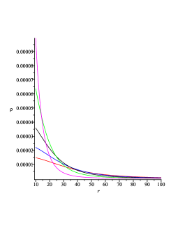
Figure 1: Plot for the variation of $\rho$ vs $r$ (in kpc). Here $R=50,40,30,20,10$ for Red, Blue, Black, Green and Magenta respectively.

The plots (Fig. 1) for variation of density with distance show interesting characteristics for the distribution of mass in galactic halo region. It is influenced by the value of $R$. The parameter $R$ indicates a scaling factor. The plots show that the density in the galactic halo region varies as inverse square of the distance. The observed flat rotation curves in the galactic halo region predict similar behavior in the distribution of masses in the region [58, 5, 6, 8].

In a similar way, from the Eqs. (4), (5) and (6) we get the expressions respectively for radial and tangential pressures in the following forms:

$$p_{r}=\frac{\omega}{8\pi(1+\omega)}\left[\frac{1}{R^{2}}\left(3+\frac{r^{2}}{R^{2}}\right)\left(1+\frac{r^{2}}{R^{2}}\right)^{-2}+\left(1+\frac{r^{2}}{R^{2}}\right)^{-1}\left(\frac{l}{r^{2}}+\frac{1}{r^{2}}\right)-\frac{1}{r^{2}}\right],$$ (16)

and

$$p_{t}=\frac{1}{8\pi}\left[\left(1+\frac{r^{2}}{R^{2}}\right)^{-1}\left\{\frac{l^{2}}{4r^{2}}-\frac{1}{1+\omega}\left(\frac{l+1}{r^{2}}\right)\right\}\right.$$

$$-\left.\frac{1}{R^{2}}\left(1+\frac{r^{2}}{R^{2}}\right)^{-2}\left\{1+\frac{l}{2}+\frac{\omega}{1+\omega}\left(3+\frac{r^{2}}{R^{2}}\right)\right\}+\frac{1}{r^{2}(1+\omega)}\right].$$ (17)

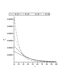
Figure 2: Plot for the variation of $p_{r}$ vs $r$ (in kpc).

Since pressure directly depends on the density of the galactic fluid, its value must be very small in galactic halo region. From Fig. 2 it may be noted that the radial pressure decreases sharply with distance from an initial large value and becomes very small after $50$ kpc. Thus our model predicts that the value of radial pressure must be very small in the galactic halo region. Though cold dark matter (CDM) models predict dark matter to be constituted of weakly interacting massive particles (WIMPS) which offers zero pressure, Bharadwaj and Kar [59] successfully modelled galactic halo considering dark matter having different pressures in radial and transverse directions. Recently Harko and Lobo [60] also proposed a model of galactic halo considering characteristic pressure of dark matter.

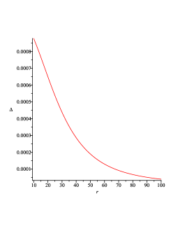
Figure 3: Plot for the variation of $\Delta=(p_{t}-p_{r})$ vs $r~{}(R=40)$ in galactic halo region.

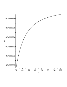
Figure 4: Plot for the variation of $\beta=(1-\frac{p_{t}^{2}}{p_{r}^{2}})$ vs $r~{}(R=30)$ in galactic halo region.

We note, from the Fig. 3, that the anisotropy in the galactic halo region gradually decreases with distance. It indicates possible deviation from spherical symmetry. Dubinsky and Carlberg [61] first observed that the halos of elliptic galaxies are rounder than the shape predicted by cold dark matter simulation. Recently Kazantzidis et al. [62] reported that cosmological simulations with cooling of baryons in the galactic halo region are rounder than the shape obtained in adiabatic simulation. They pointed out that condensation of dark matter in the galactic halo region due to cooling may result in a more spherical distribution of dark matter. In the present model we have taken the galactic halo region dominated by dark matter which is consistent with the observational evidences. Hence the predictions of our model is consistent with the cold dark matter simulations as also mentioned in the Introductory part of the present paper [47, 48, 49, 50, 51, 52, 53].

Let us now find out an expression for the electric field. This can be given by

$$F=\frac{\omega}{R^{2}(1+\omega)}\left(3+\frac{r^{2}}{R^{2}}\right)\left(1+\frac{r^{2}}{R^{2}}\right)^{-2}+\frac{1}{1+\omega}\left[\left(1+\frac{r^{2}}{R^{2}}\right)^{-1}\left(\frac{l}{r^{2}}+\frac{1}{r^{2}}\right)-\frac{1}{r^{2}}\right].$$ (18)

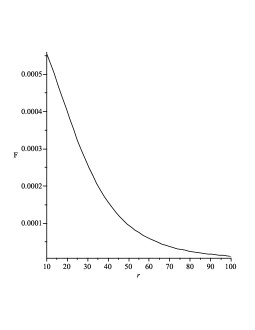
Figure 5: Plot for the variation of $F$ vs $r$ in kpc $(R=40)$ in galactic halo region.

From the Fig. 5 we observe that the electric field in the galactic halo region decreases gradually with distance from the galactic center. The distribution of charge in the galactic halo region can be noted from Fig. 6. The charge density appears to be large near the galactic center and it decreases steadily with the distance (Fig. 7).

3 Stability of orbits of neutral hydrogen clouds

Let a test particle with four velocity $U^{\alpha}=\frac{dx^{\sigma}}{d\tau}$ moving in the region of spacetime metric given in Eq. (14). Assuming $\theta=\pi/2$, the equation $g_{\nu\sigma}U^{\nu}U^{\sigma}=-m_{0}^{2}$ yields

$$\left(\frac{dr}{d\tau}\right)^{2}=E^{2}+V(r),$$ (19)

with

$$V(r)=-\left[E^{2}\left(1-\frac{1}{B_{0}r^{l}(1+\frac{r^{2}}{R^{2}})}\right)+\frac{\left(1+\frac{L^{2}}{r^{2}}\right)}{\left(1+\frac{r^{2}}{R^{2}}\right)}\right].$$ (20)

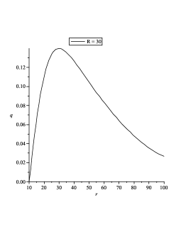
Figure 6: Plot for the total charge integrated from $r_{1}=10$ kpc and $r_{2}$ varied from $10$ kpc to $100$ kpc ($R=30$, $l=10^{-6}$, $\omega=1$) in galactic halo region.

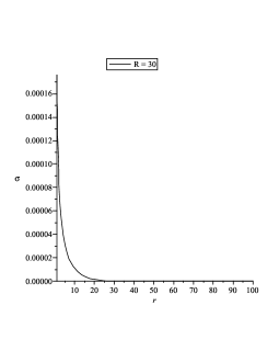
Figure 7: Plot for the variation of $\sigma$ vs $r$ in kpc ($R=30$, $l=10^{-6}$, $\omega=1$) in galactic halo region.

Here the two conserved quantities, namely relativistic energy ($E$) and angular momentum ($L$) per unit rest mass of the test particle respectively are

$$\quad E=\frac{U_{0}}{m_{0}}\quad and\quad L=\frac{U_{3}}{m_{0}}.$$ (21)

If the circular orbits are defined by $r=a$, then $\frac{da_{0}}{d\tau}=0$ and, additionally, $\frac{dV}{dr}\mid_{r=a}=0$. Above two conditions result

$$L=\pm\sqrt{\frac{l}{2-l}}a,$$ (22)

and by using $L$ in $V(a)=-E^{2}$, we get

$$E=\pm\sqrt{\frac{2B_{0}}{2-l}}a^{l/2}.$$ (23)

The orbits will be stable if $\frac{d^{2}V}{dr^{2}}\mid_{r=a}<0$ and unstable if $\frac{d^{2}V}{dr^{2}}\mid_{r=a}>0$.

By putting the expressions for $L$ and $E$ in $\frac{d^{2}V}{dr^{2}}\mid_{r=a}$, finally we get

$$\frac{d^{2}V}{dr^{2}}\mid_{r=a}=-\frac{R^{2}}{B_{0}\left(R^{2}+a^{2}\right)^{3}a^{4}}\left(-E^{2}a^{(2-l)}l^{2}R^{4}-2E^{2}a^{4-l}l^{2}R^{2}-E^{2}a^{(6-l)}l^{2}\right.$$

$$-\left.6E^{2}a^{(4-l)}lR^{2}-5E^{2}a^{(6-l)}l-E^{2}a^{(2-l)}lR^{4}6E^{2}a^{(6-l)}+2E^{2}a^{(4-l)}R^{2}\right.$$

$$+\left.6L^{2}B_{0}R^{4}+18L^{2}B_{0}R^{2}a^{2}+20L^{2}B_{0}a^{4}+6a^{6}B_{0}-2B_{0}a^{4}R^{2}\right).$$ (24)

The second derivative of the gravitational potential function is plotted for different values of the parameters $E$, $l$, $R$, $B_{0}$ and $L$. The plots are given in Figs.(8), (9) and (10). The plots show that the second derivative is negative for arbitrary ranges of $r$. So the orbits of neutral hydrogen cloud must be stable in galactic halo region. The plots reveal an important relationship between angular momentum per unit mass of the test particles and the stability of the orbits. For $L=1$ (Fig. 9) the orbits are unstable up to the distance of nearly $10$ kpc. However, for comparatively large values of $L$, the orbits are stable in the range from $10$ kpc to $300$ kpc.

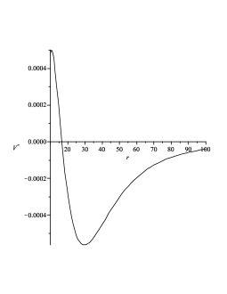
Figure 8: Plot for the variation of $V^{\prime\prime}$ vs $r$ [$L=1$, $R=30$, $l=10^{-6}$, $E=10^{-4}$, $B_{0}=100$].

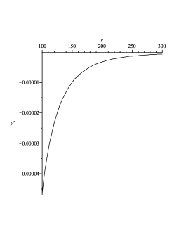
Figure 9: Plot for the variation of $V^{\prime\prime}$ vs $r$ [$L=20$, $R=30$, $l=10^{-6}$, $E=10^{-4}$, $B_{0}=100$].

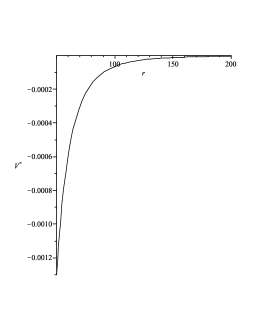
Figure 10: Plot for the variation of $V^{\prime\prime}$ vs $r$ [$L=40$, $R=30$, $l=10^{-6}$, $E=10^{-4}$, $B_{0}=100$].

4 Motion of test particles in galactic halo region

Since the observations indicate that gravity in the galactic scale would be attractive, therefore, it is interesting to check whether the particles are being accelerated towards the galactic center. Geodesic study will help to see this important characteristic.

Now we study the geodesic equation for a test particle that has been “placed” at some radius $r_{0}$ and is given by

$$\frac{d^{2}x^{\alpha}}{d\tau^{2}}+\Gamma_{\alpha}^{\mu\gamma}\frac{dx^{\mu}}{d\tau}\frac{dx^{\gamma}}{d\tau}=0.$$ (25)

This yields the radial equation

$$\frac{d^{2}r}{d\tau^{2}}=-\frac{1}{2}\left(1+\frac{r^{2}}{R^{2}}\right)^{-1}\left[\frac{d}{dr}\left(1+\frac{r^{2}}{R^{2}}\right)\left(\frac{dr}{d\tau}\right)^{2}+\frac{d}{dr}B_{0}r^{l}\left(\frac{dt}{d\tau}\right)^{2}\right].$$ (26)

Since $\left(\frac{dr}{d\tau}\right)_{r=r_{0}}=0$ for a stable orbit, we find from equation (26)

$$\frac{d^{2}r}{d\tau^{2}}=-\frac{1}{2}\frac{1}{\left(1+\frac{r^{2}}{R^{2}}\right)}B_{0}lr^{l-1}\left(\frac{dt}{d\tau}\right)^{2}<0.$$ (27)

Thus particles are attracted towards the center. Interestingly, since we are considering the rotation of neutral hydrogen clouds, the electric field will have no direct effect on the motion. However, the electric field contributes to the energy-momentum tensor of the system which in turn influences the geometry of the space-time. Thus, the electric field indirectly affects the motion of the neutral hydrogen clouds.

5 The total gravitational energy

We try to find out the total gravitational energy $E_{G}$ between two fixed radii, say, $r_{1}$ and $r_{2}$ which is given by

$$E_{G}=M-E_{M}=4\pi\int_{r_{1}}^{r_{2}}\left[1-\sqrt{\left(1-\frac{r^{2}}{R^{2}}\right)}\right]\rho r^{2}dr.$$

This study will be interesting as positive energy density does not always lead to attractive gravity [16]. According to Misner, Thorne and Wheeler [63] and Nandi et al. [16] the total gravitational energy in the halo region should be negative.

Now, plugging $\rho$ from Eq. (15), we get for the total gravitational energy $E_{G}$ as follows:

$$E_{G}=4\pi\int_{r_{1}}^{r_{2}}\left[1-\sqrt{\left(1-\frac{r^{2}}{R^{2}}\right)}\right]\times$$

$$\left[\frac{1}{8\pi(1+\omega)}\left\{\frac{1}{R^{2}}\left(3+\frac{r^{2}}{R^{2}}\right)\left(1+\frac{r^{2}}{R^{2}}\right)^{-2}+\left(1+\frac{r^{2}}{R^{2}}\right)^{-1}\left(\frac{l+1}{r^{2}}\right)-\frac{1}{r^{2}}\right\}\right]r^{2}dr,$$ (28)

where

$$M=\left(\frac{1}{2(1+\omega)}\right)\int_{r_{1}}^{r_{2}}\left[\frac{1}{R^{2}}\left(3+\frac{r^{2}}{R^{2}}\right)\left(1+\frac{r^{2}}{R^{2}}\right)^{-2}\right.$$

$$+\left.\left(1+\frac{r^{2}}{R^{2}}\right)^{-1}\left(\frac{l+1}{r^{2}}\right)-\frac{1}{r^{2}}\right]r^{2}dr,$$ (29)

i.e. the Newtonian mass can be expressed as

$$M=\frac{1}{8(1+\omega)}\left[R(l+1)\tan^{-1}\left(\frac{r}{R}\right)-R^{2}\left(\frac{r}{R^{2}+r^{2}}\right)\right]_{r{1}}^{r{2}}.$$ (30)

Thus we get the total gravitational energy as follows:

$$E_{G}=\frac{1}{2(1+\omega)}\left[R(l+1)\tan^{-1}\left(\frac{r}{R}\right)-\frac{R^{2}r}{r^{2}+R^{2}}-R(l+2)\log|r+\sqrt{R^{2}+r^{2}}|\right.$$

$$+\left.\frac{2Rr}{\sqrt{R^{2}+r^{2}}}\right]_{r_{1}}^{r_{2}}.$$ (31)

Figs. (11) and (12) show that the total gravitational energy in the galactic halo region is negative for arbitrary choice of positive values of $r_{1}$ and $r_{2}$. It may be noted this is consistent with the present day observations.

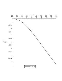
Figure 11: Plot for the total gravitational energy $E_{g}$ vs $r$ in Kpc.

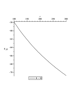
Figure 12: Plot for the total gravitational energy $E_{g}$ vs $r$ in Kpc.

6 The observed equation of state

From the gravitational lensing measurements and the gravitational potential and total mass-energy inferred from the rotational curves we can approximately obtain a dimensionless parameter which gives the rough measure of the equation of state of the fluid in the galactic halo region [64]. But first of all let us rewrite the metric of static, spherically symmetric spacetime as given in Eq. (1), in the following form:

$$ds^{2}=-e^{2\phi(r)}dt^{2}+\frac{1}{1-2m(r)/r}dr^{2}+r^{2}d\Omega_{2}^{2},$$ (32)

where $m(r)$ and $\phi(r)$ are two functions which determine the metric uniquely. Comparing the above metric (32) with the metric (1), we get

$$\phi(r)=\frac{1}{2}\left[\ln B_{0}+l\ln r\right],$$ (33)

and

$$m(r)=\frac{1}{2}\left[\frac{r^{3}}{R^{2}+r^{2}}\right].$$ (34)

From the Einstein’s field equations for the metric (32), $m(r)$ can be interpreted as the total mass-energy within a spherical distribution of radius $r$ and $\phi(r)$ is the gravitational potential. From the Fig. 13 we can note that function $m(r)$ increases with $r$. The plot resembles the plot of cumulative mass versus radius in the paper of van Albada et al. [65].

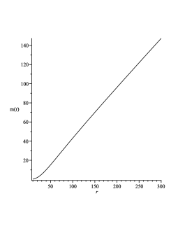
Figure 13: Plot for the variation of $m(r)$ vs $r$ in Kpc.

Now, let us define $\Phi(r)_{RC}$ as the gravitational potential obtained from the measurements of rotational curves. Since the test particles moving in the galactic halo region are governed by the general relativistic potential $\Phi(r)$, therefore one can conclude $\Phi(r)=\Phi_{RC}(r)$. Similarly, $m_{RC}(r)$ is defined as the mass obtained from the rotational curve measurements. As given by Faber and Visser [64], the values of these functions are:

$$\phi_{RC}=\phi(r)=\frac{l}{2r},$$ (35)

and

$$m_{RC}=r^{2}\Phi^{\prime}(r)=\frac{1}{2}lr.$$ (36)

The primes denote the derivatives with respect to $r$. The quantity $m_{RC}$ represents the mass estimate from the rotational curves. It is interesting to note from the aforementioned equation that $m_{RC}\propto r$ (Fig. 14). This is in conformity with the observational evidences.

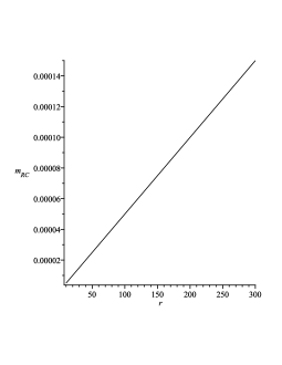
Figure 14: Plot for the variation of $m_{RC}$ vs $r$ in Kpc.

As discussed in Nandi et al. [16], the functions are determined indirectly from certain lensing measurements defined by

$$\Phi_{lens}=\frac{\Phi(r)}{2}+\frac{1}{2}\int\frac{m(r)}{r^{2}}dr=\frac{\ln B_{0}}{4}+\frac{l\ln r}{4}+\frac{\ln(r^{2}+R^{2})}{8},$$ (37)

and

$$m_{lens}=\frac{1}{2}r^{2}\Phi^{\prime}(r)+\frac{1}{2}m(r)=\frac{lr}{4}+\frac{r^{3}}{4\left(R^{2}+r^{2}\right)}.$$ (38)

Of particular interest to us is the dimensionless quantity

$$\omega(r)=\frac{2}{3}\frac{m_{RC}^{\prime}-m_{lens}^{\prime}}{2m_{lens}^{\prime}-m_{RC}^{\prime}},$$ (39)

due to Faber and Visser [64]. In the above expression the subscript $RC$ refers to the rotation curve. Thus, the resulting expression is

$$\omega(r)=\frac{2}{3}\frac{m_{RC}^{\prime}-m_{lens}^{\prime}}{2m_{lens}^{\prime}-m_{RC}^{\prime}}=\frac{l\left(R^{2}+r^{2}\right)^{2}}{3\left(3r^{2}R^{2}+r^{4}\right)}.$$ (40)

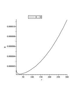
Figure 15: Variation of observed equation of state parameter $\omega(r)$ with $r$ in kpc. $R=30$

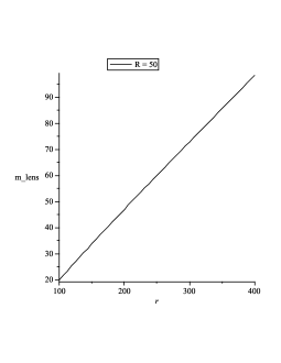
Figure 16: Variation of $m_{lens}$ with $r$ in kpc. $R=50$, $B_{0}=100$

As we can note from the Fig. 15 that the observed equation of state parameter in the galactic halo region is always positive. This indicates that the matter content in the galactic halo region must be normal matter. This is in confirmation with the earlier works of Rahaman et al. [19].

On the other hand, small variation of observed equation of state parameter with distance is shown in the plot (Fig. 16). The parameter $m_{lens}$ represents pseudo mass in the galactic halo region contributing to lensing potential, $\Phi_{lens}$ [64]. The Fig. 16 shows steady increase in $m_{lens}$ in the galactic halo region $\left(m_{lens}\propto r\right)$. We should remember that $m_{lens}$ is the mass to be observed in the halo region. The observations also predict linear increase in mass in the galactic halo $\left(M(r)\propto r\right)$. Thus the predictions of the model is supported by observational evidences.

7 Post Newtonian mass in galactic halo region

In Newtonian regime the pressures of galactic fluids are to be negligible [64]. We have calculated the Newtonian mass of the galactic fluid in Eq. (30). The post Newtonian mass of the galactic fluid is given by the following equation

$$M_{pN}=4\pi\int_{r_{1}}^{r_{2}}(\rho+p_{r}+2p_{t})r^{2}dr.$$

Thus, after plugging the parameters $\rho$, $p_{r}$, $p_{t}$ and performing integration, we get the post Newtonian mass of the galactic fluid in the following form:

$$M_{pN}=\left[\frac{1}{2}\left\{R(l+1)\tan^{-1}\left(\frac{r}{R}\right)-\frac{rR^{2}}{r^{2}+R^{2}}\right\}+\left(\frac{l^{2}-l-2}{4}-\frac{l+1}{\omega+1}\right)R\tan^{-1}\left(\frac{r}{R}\right)\right.$$

$$+\left.\left(\frac{l+2}{4}+\frac{\omega}{1+\omega}\right)\frac{R^{2}r^{2}}{R^{2}+r^{2}}-\frac{\omega r}{1+\omega}\right]_{r_{1}}^{r_{2}}.$$ (41)

As can be noted from the plots of Newtonian and post Newtonian mass (Figs. 16-19), both increases linearly with distance from $100$ kpc to $300$ kpc. The Figs. 17 and 18 show that the Newtonian mass increases nonlinearly up to $60$ kpc from the galactic center. Beyond that the increase becomes linear with distance.

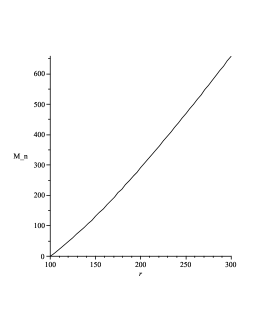
Figure 17: Plot for the Newtonian mass $M_{N}$ vs $r$ (in kpc) in galactic halo region with different range.

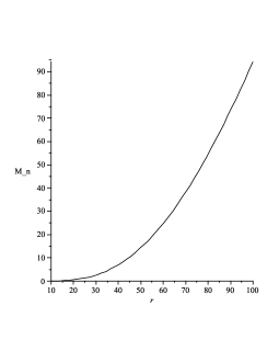
Figure 18: Plot for the Newtonian mass $M_{N}$ vs $r$ (in kpc) in galactic halo region with different range.

On the other hand, the increase of post Newtonian mass becomes linear from $30$ kpc from galactic center (Figs. 19 and 20). This implies that in the halo region Newtonian as well as post Newtonian mass is proportional to $r$. The observational predictions from the rotational curves in the galactic halo region are also in accordance with this result. From numerical simulation we found that the ratio of post Newtonian to Newtonian mass of galactic fluid in the range $100$ kpc to $300$ kpc is nearly $659.7984402$. In the range $10$ kpc to $100$ kpc the post Newtonian mass is nearly $1125.448032$ times larger than Newtonian mass. Since the post Newtonian mass indicates the relativistic effect, one can note from the figures that relativistic effects are considerable in the galactic halo region.

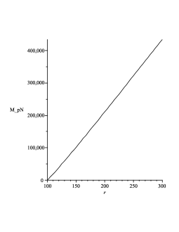
Figure 19: Plot for the post Newtonian mass $M_{pN}$ vs $r$ (in kpc) in galactic halo region with different range.

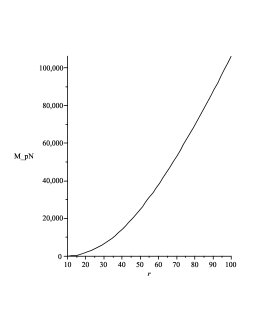
Figure 20: Plot for the post Newtonian mass $M_{pN}$ vs $r$ (in kpc) in galactic halo region with different range.

8 Concluding Remarks

In the foregoing, we have proposed a model of galactic halo with electric field. The motivation behind such proposal is that only Einstein’s General Theory of Relativity fail to explain the observed phenomena of the rotation curves of spiral galaxies. Researchers need to hypothesize the existence of some non luminous dark matter of unknown properties to be responsible for this peculiar phenomena. The assumption that ‘mass increases with radial distance’ may support the observed result, however, luminous mass distribution does not follow this behavior. We have proposed the model of galactic halo with electric field rather considering the unknown nature of the dark matter.

Different cosmological models (e.g. SCDM, $\Lambda$-CDM etc.) predict attractive gravity in galactic halo region and beyond. We have confirmed the existence of attractive gravity in the halo region (Sec. 5). The orbits of revolving particles are found to be stable in the halo. However, in the region within $10$ kpc from galactic center, the orbits are unstable for particles of comparatively small angular momentum per unit mass. For Milky way galaxy this region belongs to the stellar halo region.

The geometry of the halo region is calculated from the observational constraint. The results of the present paper show that being considered as a fluid, possibly, dark matter is not exotic in nature. However, from the point of view of particle physics what dark matter is constituted of is yet to be resolved. Our results has nothing to remark on the particle aspect of the dark matter. The pressure of dark matter as predicted in SCDM paradigm is negligible. We have confirmed this theoretical prediction in our results. The observational features predicted here (Sec. 6) are also in agreement with the present observational evidences regarding galactic halo.

The present model indicates that in the halo region Newtonian as well as post Newtonian mass is proportional to $r$. The observational predictions from the rotational curves in the galactic halo region are also in accordance with this result. From numerical simulation we found that the ratio of post Newtonian to Newtonian mass of galactic fluid in the range $100$ kpc to $300$ kpc is nearly $659$. Though the post Newtonian mass indicates the relativistic effect, taking into consideration the large distance scale in the galactic halo, one can note that relativistic effects will not be appreciably high in the galactic halo region. Thus interestingly, we find in our model that $M_{pN}\approx 659M(r)$ in contrast to the well known scalar field model $M_{pN}=10^{6}M(r)$ [66]. As per observational evidences, the interaction cross-section of dark matter with normal baryonic matter must be very small. Commonly referred dark matter particle candidates like WIMP, axions etc. also supports the prediction [67]. Since we have taken the baryonic matter content in the galactic halo region negligible compared to the dark matter, the present model predicts that the role of electric field in anisotropy of galactic halo must be very weak.

A proper relativistic model of galactic halo with electric field must be based on electrohydrodynamics. However, ours is a simpler model in which we have assumed the motion of charged particles within the galactic halo insignificant. Also, the magnetic field is assumed much less than the electric field. Commonly, magnetic field is regarded as significant in halos. However, with the assumptions aforementioned, it is shown that the model predicts successfully some of the observational features regarding galactic halo. This model can be extended farther with the help of electro-hydrodynamics and electromagneto-hydrodynamics.

The present work may be extended by considering magnetic field along with the electric field. A more realistic model of galactic halo may be thought of with the superposition of halo with galactic disc [70, 71, 72] or central black hole [73, 74, 75].

References

- [1] Oort, J.: Bull. Astron. Inst. Neth. VI 249, 249 (1932)
- [2] Zwicky, F.: Helvet. Phys. Acta 6, 110 (1933)
- [3] Zwicky, F.: ApJ 86, 217 (1937)
- [4] Freeman, K.C.: ApJ 160, 881 (1970)
- [5] Roberts, M.S., Rots, A.H.: Astron. Astrophys. 26, 483 (1973)
- [6] Ostriker, P., Peebles, P.J.E., Yahill, A.: ApJ 193, L1 (1974)
- [7] Einasto, J., Kaasik, A., Saar, E.: Nat. 250, 309 (1974)
- [8] Rubin, V.C., Thonnard, N., Ford Jr., W.K.: ApJ 225 L107 (1978)
- [9] Sofue, Y., Rubin, V.: Ann. Rev. Astron. Astrophys. 39, 137 (2001)
- [10] Jugman, G., Kamionkowski, M., Griest, K.: Phys. Rep. 267, 195 (1996)
- [11] Efstathiou, G., Sutherland, W., Madox, S.J.: Nature 348, 705 (1990)
- [12] Pope, A.C., et al.: ApJ 607, 655 (2004)
- [13] Tegmark, M., et al.: Phys. Rev. D 69, 103501 (2004)
- [14] Tegmark, M., et al.: ApJ 606, 702 (2004)
- [15] Rahaman, F., Kalam, M., DeBenedictis, A., Usmani, A., Ray, S.: MNRAS 389, 27 (2008)
- [16] Nandi, K.K., Filippov, A.I., Rahaman, F., Ray, S., Usmani, A.A., Kalam, M., DeBenedictis, A.: MNRAS 399, 2079 (2009)
- [17] Rahaman, F., Kuhfittig, P.K.F., Amin, R., Mandal, G., Ray, S., Islam, N.: Phys. Lett. B 714, 131 (2012)
- [18] Rahaman, F., Kuhfittig, P.K.F., Ray, S., Islam, N.: Eur. Phys. J. C 74, 2750 (2014)
- [19] Rahaman, F., Nandi, K.K., Bhadra, A., Kalam, M., Chakraborty, K.: Phys. Lett. B 694, 10 (2010)
- [20] Pannekoek, A.: Bull. Astron. Inst. Neth. 1, 107 (1922)
- [21] Rosseland, S.: MNRAS 84, 720 (1924)
- [22] Eddington, A.S.: The Internal Constitution of the Stars, Cambridge University Press, New York (1926)
- [23] Cowling, T.G.: MNRAS 90, 140 (1929)
- [24] Shvartsman, V.F.: Sov. Phys. JETP 33, 475 (1971)
- [25] Neslus̆an, L.: Astron. Astrophys. 372, 913 (2001)
- [26] Hall, L.J.: ’86 Massive Neutrinos in Astrophysics and in Particle Physics, Proceedings of the 6th Moriond Workshop, Tignes, Savoie, France, January 25-February 1st, 1986 (Ed. O. Fackler and J. Tran Thanh Van. Gif-sur-Yvette: Editions Frontieres, 1986., p.93)
- [27] Berezhiani, Z., Dolgov, A.D., Tkachev, I.I.: Eur. Phys. J. C 73, 2620 (2013)
- [28] Harari, D., Mollerach, S., Roulet, E.: JCAP 11, 033 (2010)
- [29] Lake, K.: Phys. Rev. D 80, 064039 (2009)
- [30] Herrera, L., Barreto, W.: Phys. Rev. D 88, 084022 (2013)
- [31] Herrera, L., Ospino, J., Di Prisco, A.: arXiv:0712.0713v3 [gr-qc] (2008)
- [32] Nguyen, P.H., Lingam, M.: MNRAS 436, 2014 (2013)
- [33] Sgró, M.A., Paz, D.J., Merchán, M.: arXiv:1305.0563v1 [astro-ph.CO], DOI: 10.1093/mnras/stt773 (2013)
- [34] Nguyen, P.H., Pedraza, J.F.: Phys. Rev. D 88, 064020 (2013)
- [35] Howk, J.C., Consiglio, S.M.: ApJ 759, 97 (2012)
- [36] Meiksin, A.A.: Rev. Mod. Phys. 81, 1405 (2009)
- [37] Tripp, T.M., Savage, B.D., Jenkins, E.B.: ApJ 534, L1 (2000)
- [38] Savage, B.D., et al.: ApJ Supple. 146, 125 (2003)
- [39] Yao, Y.S., Wang, Q.D.: ApJ 624, 751 (2005)
- [40] Lehner, N., Savage, B.D., Walker, B.P., Sembach, K.P., Tripp, T.M.: ApJ 164, 1 (2006)
- [41] Yao, Y.S., Wang, Q.D.: ApJ 658, 1088 (2007)
- [42] Tripp, T.M., et al.: ApJ Supple 177, 39 (2008)
- [43] Yao, Y.S., Wang, Q.D., Hagihara, T., Mitsuda, K., McCamon, D., Yamasaki, N.Y.: ApJ 690, 143 (2009)
- [44] Yao, Y.S., Wang, Q.D., Penton, S.V., Shull, J.M., Strocke, J.T.: ApJ 716, 1514 (2010)
- [45] Danforth, C.W., Shull, J.M., Rosenberg, J.L., Strocke, J.T.: ApJ 640, 716 (2006)
- [46] Fraternali, F., Binney, J., Oosterloo, T., Sancisi, R.: ApJ 653, 1517 (2006)
- [47] Navaro, J.F., Frenk, C.S., White, S.D.M.: ApJ 462, 563 (1996)
- [48] Navaro, J.F., Frenk, C.S., White, S.D.M.: ApJ 490, 493 (1997)
- [49] Fukushinge, T., Makino, J.: ApJ 477, L9 (1997)
- [50] Fukushinge, T., Makino, J.: ApJ 577, 533 (2001)
- [51] Jing, Y.P.: ApJ 535, 30 (2000)
- [52] Jing, Y.P., Suto, Y.: ApJ 574, 538 (2002)
- [53] Lux, H., Read, J.I., Lak, G., Johnston, K.V.: MNRAS 424, L16 (2012)
- [54] Finch, M.R., Skea, J.E.F.: 1989, Class. Quant. Grav. 6, 467 (1989)
- [55] Jotania, K., Tikekar, R.: Int. J. Mod. Phys. D 15, 1175 (2006)
- [56] Landau, L.D., Lifshitz, E.M.: Classical Theory of Fields, Butterworth-Heineman (1998)
- [57] Nucamendi, U., Salgado, M., Sudarsky, D.: Phys. Rev. D 63, 125016 (2001)
- [58] Rubin, V.C., Ford Jr., W.K.: ApJ 159, 379 (1970)
- [59] Bharadwaj, S., Kar, S.: Phys. Rev. D 68, 023516 (2003)
- [60] Harko, T., Lobo, F.S.N.: Astropart. Phys. 35, 547 (2012)
- [61] Dubinsky, J., Carlberg, R.G.: ApJ 378, 496 (1991)
- [62] Kazantzidis, S., Kravtsov, A.V., Zentner, A.R., Allgood, B.: ApJ 611, L73 (2004)
- [63] Misner, C.W., Thorne, K.S., Wheeler, J.A.: Gravitation, Freeman, San Franscisco (1973)
- [64] Faber, T., Visser, M.: MNRAS 372, 136 (2006)
- [65] van Albada, T.S., Bahcall, J.N., Begeman, K., Sanscisi, R.: ApJ 295, 305 (1985)
- [66] Matos, T., Guzman, S.F.: Phys. Rev. D 62, 061301 (2000)
- [67] Overduin, J.M., Wesson, P.S.: Phys. Repts. 402, 267 (2004)
- [68] Bally, J., Harrison, E.R.: ApJ, 220, 743 (1978)
- [69] de Diego, J.A., Dultzin-Hacyan, D., Trejo, J.G., Núnez, D.: arXiv: astro-ph/0405237v1 (2004)
- [70] Vogt, D., Letelier, P.S.: Phys. Rev. D 68, 084010 (2003)
- [71] Lora-Clavijo, F.D., Ospina-Henao, P.A., Pedraza, J.F.: Phys. Rev. D 82, 084005 (2010)
- [72] Gutiérrez, A.C., González, G.A., Quevedo, H.: arXiv:1211.4941v2 [gr-qc] (2012)
- [73] Semerák, O.: Gravitation: Following the Prague Inspiration (To celebrate the 60th birthday of Jiri Bicak), Eds. Semerak, O., Podolsky, J., Zofka, M. (World Scientific, Singapore 2002), p. 111, arXiv:gr-qc/0204025v1 (2002)
- [74] Vogt, D.: Phys. Rev. D 71, 044009 (2005)
- [75] Guitiérrez-Piñeres, AC., García-Reyes, G., Gozález, G.A.: Int. J. Mod. Phys. D 23 1450010-1 (2013)