Time stretching of the GeV emission of GRBs: Fermi-LAT data vs geometrical model

Abstract

It is known that the high energy $(>100\,\mathrm{MeV})$ emission of gamma-ray bursts is delayed with respect to the low energy emission. However, the dependence of light curves on energy has not been studied for the high energy bands. In this paper we consider the bursts observed by Fermi LAT from 2008 August 4 to 2011 August 1, for which at least $10$ photons were observed with the energy greater than $1\,\mathrm{GeV}$. These include $4$ bursts: GRB 080916C, GRB 090510, GRB 090902B, and GRB 090926A. We use the Kolmogorov-Smirnov test to compare the light curves in the two bands, $100\,\mathrm{MeV}<E<1\,\mathrm{GeV}$ and $E>1\,\mathrm{GeV}$. For GRB 080916C and GRB 090510 the light curves in the two bands are statistically compatible. However, for GRB 090926A, the higher-energy light curve is stretched compared to the lower-energy one with a statistical significance of $3.3\sigma$ and, for GRB 090902B, on the contrary, the lower-energy curve is stretched with $2.3\sigma$ significance. We argue that the observed diversity of stretching factors may be explained in a simple geometrical model. The model assumes that the jet opening angle depends on the emission energy in a way that the most energetic photons are radiated near the axis of the jet. All the bursts are considered equivalent in their rest frames and the observed light curves differ only due to different redshifts and view directions. The model conforms to the total burst energy constraint and matches the Fermi-LAT observations of the fraction of GRBs visible in $100\,\mathrm{MeV}<E<1\,\mathrm{GeV}$ band, which may be observed at higher energies. The model predicts the distribution of observable stretching factors, which may be tested in the future data. Finally, we propose a method to estimate observer’s off-axis angle based on the stretching factor and the fraction of the high-energy photons. The code for modeling is open source and is publicly available on GitHub (https://github.com/maxitg/GammaRays).

1 Introduction and summary

Gamma-ray bursts (GRBs) are among the most energetic events in the Universe. Therefore, the studies of the emission mechanism and phenomenology of GRBs may provide the new knowledge in particle physics. Moreover, the GRBs are observed from cosmological distances and therefore bear an imprint of the late-time evolution of the Universe. An extensive studies of these explosions led to a number of interesting results, see [1, 2] for a review. In particular, the total energy emitted in gamma-rays during a burst was found to be similar for the different GRBs within an order of magnitude [3]. This indicates that the most of the bursts have similar energetics in their rest frames. Moreover, the high energy radiation of GRBs is shown to follow the predictions of the synchrotron radiation scenario [4]. Several observations are related to the temporal variations of spectra. This way, the spectral lags were found between different low energy bands [5] and the very-high-energy radiation was discovered to be extended relative to the x-ray emission [6, 7, 1]. In this paper we go further and compare the temporal extension of GRB gamma-ray radiation in the two energy bands $100\,\mathrm{MeV}<E<1\,\mathrm{GeV}$ and $E>1\,\mathrm{GeV}$ (hereafter, low and high-energy bands) using the data from the Large Area Telescope (LAT) of the Fermi satellite [8, 9].

We start with the location, time and duration of bursts from the Fermi-LAT Gamma-Ray Burst Catalog [10]. The photons during the burst and the photons for 24 hours before the burst are downloaded from the LAT Data Server . The latter are used for the background estimation in both energy bands with the technique introduced in [11]. In order to have enough statistics we require that at least 10 photons are detected with the energy greater than $1\,\mathrm{GeV}$. This leaves us with the four bursts for the time span of the Fermi-LAT Gamma-Ray Burst Catalog. Namely, GRB 080916C [12], GRB 090510 [13], GRB 090902B [14] and GRB 090926A [15]. For these bursts we stretch the high energy light curve by the arbitrary factor and compare with the low energy light curve using the Kolmogorov-Smirnov (KS) test. Within the $95\%$ confidence level the stretching factor is compatible to $1$ (no stretching) for the GRB 080916C and GRB 090510. For the other two bursts the stretching factor of 1 is, however, excluded. For GRB 090902B it should be smaller than 1, so the low energy light curve is stretched with respect to the high energy one, see fig. 5. Even more significant deviation from the stretching factor of 1 in the opposite direction is observed for the GRB 090926A. The high energy light curve of GRB 090926A is stretched with respect to the low energy one by a factor of at least 1.99 (see fig. 6). The stretching of the GRB 090926A high energy light is found with $3.3\sigma$ significance. All the observed stretching factors are summarized in Table 2, and the detailed procedure for their calculation is described in Section 2.

We propose that the observed energy dependence of the time profiles may be explained without introduction of the new effects. We argue that the stretching may originate from the effects of the jet geometry called curvature effects. These effects were explored by multiple authors [16, 17, 18]. These studies concerned x-ray radiation, and considered the homogeneous distribution of radiation sources throughout the jet. Our model is based on the reverse assumption that the highest energy radiators are concentrated near the axis of the jet and consequently the jet opening angle depends on energy. The latter is motivated by observations if all bursts are considered equivalent. In this case the energy dependence of the jet opening angle resolves the contradiction between the small fraction of GRBs visible above GeV and the hard spectrum.

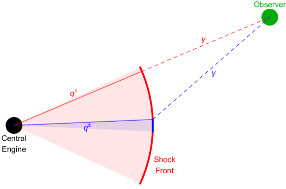
Figure 1: Model Overview. The red and blue cones represent the regions through which low and high energy charged particles propagate. In the case shown the observer’s off-axis angle is smaller than the opening angle of the low energy jet, so, due to the relativistic beaming effect, the most of the observable low energy photons will travel along the straight line from the central engine. Also, the observer’s off-axis angle is larger that the opening angle of the high energy jet, but the high energy radiation will still originate near the center of the jet as this is the only place where the high energy radiators are located. The observation time of a photon is a sum of two terms. First, the time interval spent in plasma as a radiator which approximately equals to the distance from the central engine to the point of emission. Second, the time interval from emission to detection which equals to the distance from the point of emission to the observer’s location. For the given position of the observer the sum is larger for high energy photons. Therefore, the high energy emission will be observed later throughout the burst duration and the high energy light curve will be stretched.

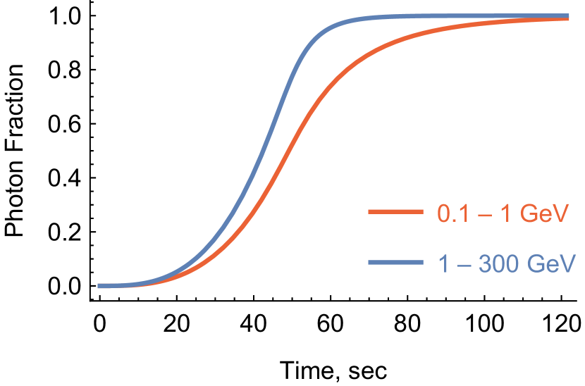
(a) Stretching factor $\kappa=0.819$, redshift $z=1.82$, off-axis angle $\chi=0$.

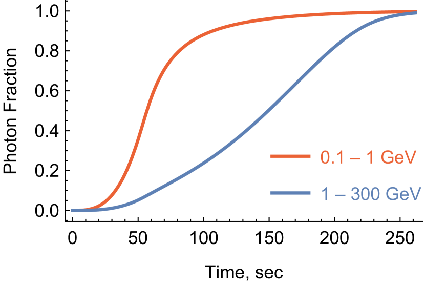
(b) Stretching factor $\kappa=2.43$, redshift $z=2.106$, off-axis angle $\chi=5.90\times 10^{-3}$.

Figure 2: High and low energy light curves produced by the geometrical model. Burst parameter values are the same as discussed in Section 5.1.

The basic idea of the model is illustrated in Figure 1. The model explains both the stretching factors lower and higher than 1 with the difference of the position of the observer with respect to the burst. The sample light curves are shown in Figure 2. The detailed calculations show that the stretching factors of GRB 090902B and GRB 090926A appear naturally in the model. The predicted distribution of stretching factors is shown in Figure 7.

The rest of the paper is organized as follows. We describe the Fermi LAT data and the analysis procedures in Section 2. The model and the details on calculations are explained in Section 3. The Section 4 introduces three phenomenological tests for the model. The parameters of the model and the new method for estimating the jet observation angles are shown in Section 5. The code for modeling is open source and is publicly available on GitHub (https://github.com/maxitg/GammaRays).

2 Data analysis

2.1 Fermi-LAT Photon Selection

GRB	$\mathrm{GBM\ Trigger\ Time}$	$\mathrm{R.A.}$	$\mathrm{Dec.}$	$\mathrm{Location\ Error}$	$T_{05}$	$T_{95}$
Name	$\mathrm{MET,\ sec}$	$\mathrm{J2000,\ deg}$	$\mathrm{J2000,\ deg}$	$\mathrm{deg}$	$\mathrm{sec}$	$\mathrm{sec}$
name	time	location.ra	location.dec	location.err	startOffset	endOffset
080825C	$241\,366\,429.105$	$233.9$	$-4.5$	$0.75$	$3.2$	$29.4$
080916C	$243\,216\,766.614$	$119.85$	$-56.64$	$0.0001$	$5.0$	$209.8$
081006	$244\,996\,175.173$	$136.32$	$-62.05$	$0.52$	$0.7$	$115.0$
081024B	$246\,576\,161.864$	$322.95$	$21.2$	$0.22$	$0.1$	$191.0$
090217	$256\,539\,404.560$	$204.83$	$-8.42$	$0.35$	$6.2$	$68.0$
090323	$259\,459\,364.630$	$190.71$	$17.053$	$0.0001$	$15.9$	$293.9$
090328	$259\,925\,808.510$	$90.67$	$-41.715$	$0.0002$	$18.8$	$652.9$
090510	$263\,607\,781.971$	$333.55$	$-26.583$	$0.0004$	$0.6$	$45.6$
090626	$267\,683\,530.880$	$170.03$	$-33.49$	$0.22$	$52.2$	$299.9$
090902B	$273\,582\,310.313$	$264.94$	$27.324$	$0.001$	$7.7$	$825.0$
090926A	$275\,631\,628.990$	$353.4$	$-66.32$	$0.01$	$5.5$	$225.0$
091003	$276\,237\,347.585$	$251.52$	$36.625$	$0.0005$	$3.9$	$452.6$
091031	$278\,683\,230.850$	$71.49$	$-57.65$	$0.23$	$3.1$	$206.2$
100116A	$285\,370\,262.240$	$305.01$	$14.43$	$0.17$	$3.0$	$141.0$
100414A	$292\,904\,423.990$	$192.11$	$8.693$	$0.0005$	$17.4$	$288.6$
110120A	$317\,231\,981.230$	$61.5$	$-12.0$	$0.36$	$0.5$	$112.8$
110428A	$325\,675\,112.410$	$5.59$	$64.849$	$0.000\,01$	$10.7$	$407.6$
110721A	$332\,916\,465.760$	$333.2$	$-38.5$	$0.20$	$0.1$	$239.0$
110731A	$333\,803\,371.954$	$280.504$	$-28.537$	$0.0001$	$3.0$	$24.1$

Table 1: Burst data used in our study taken from [10]. The third row contains the corresponding GRBurst class variable names of the software package https://github.com/maxitg/GammaRays/blob/master/GRObservations/bursts

First, we download the Pass 7REP (V15) “SOURCE” class photons from the Fermi-LAT data server [8, 9]. In order to define the regions of interest we use the catalog [10], which contains all the bright gamma-ray bursts seen by the Fermi LAT since 2008 August 4 to 2011 August 1. Specifically, we take 4 pieces of information from the tables 2 and 4 of Ref. [10]:

• GBM trigger time. It is used as a reference point for the GRB time.

• Location of the GRB. The burst locations are used to filter out photons coming from the other sources.

• Location error. Location errors are used to improve the accuracy of filtering, specifically to avoid losing statistics by filtering too much.

• $T_{05}$ – $T_{95}$ interval of the LAT-detected emission. The beginning of the interval is used as a fixed point of stretching. The Fermi-LAT photons are downloaded for the period extended in time by $50\%$ towards both past and future compared to this interval.

The data are summarized in Table 1. For the background estimation, we also download observational data for 24 hours before the burst. The analysis is performed with the Fermi Science Tools v9r33p0 package  following the guidelines . We require Earth zenith angle to be below $100^{\circ}$ to remove the Earth limb emission. After the basic filtering by gtselect and gtmktime tools is done we perform more elaborate selection using the point spread function of Fermi LAT, calculated with gtpsf tool. We use 300 energy bins from 100 MeV to 300 GeV, and 300 angular bins with maximal angle being $30\degree$. The gtltcube tool is used to compute required livetime maps. Note, that we calculate PSFs separately for both conversion types: front and back. We define $\mathrm{PSF}_{95}$ as an angular distance from the source containing 95% of the emitted photons. We require that the photon is closer than $\mathrm{PSF}_{95}+\texttt{location.err}$ to the location of the GRB (see Table 1). The details of the data request and analysis are given in appendix A.

The set will be used for the analysis with the reservation that it unavoidably contains some background photons. We consider the background flux constant in time and estimate it using the data for 24 hours before the burst. In order to calculate the number of background photons we need an exposure map, which will be discussed in the following section.

2.2 Exposure Maps and Background Estimation

The exposure map is computed with the gtexpcube2 tool. We compute it with 300 energy bins from 100 MeV to 300 GeV. The produced expcube files contain exposures as functions of energy and location on the sky. We use trilinear interpolation to compute exposures for all energies and locations. Knowing the exposures, we use the method introduced in the appendix of [11] to estimate the background for low and high-energy bands. Note, that the “TRANSIENT” class photons are not included in the analysis due to the strong dependence of the background on the spacecraft position.

2.3 KS-test

Before applying the KS-test we subtract the background, which is considered linear for the duration of the burst :

$$\Phi_{i}\left(t\right)=\frac{p_{i}\left(T_{1},t\right)-b_{i}\frac{t-T_{1}}{T_{2}-T_{1}}}{p_{i}\left(T_{1},T_{2}\right)-b_{i}}$$ (1)

Here $\left(T_{1},T_{2}\right)$ is the time range of observations, $p_{i}\left(t_{1},t_{2}\right)$ is the number of photons observed in the time range $t_{1}$ to $t_{2}$ in the $i$’s energy band ($i$ is either low or high for the low and high-energy bands respectively), and $b_{i}$ is the estimated number of background photons for the time range $T_{1}$ to $T_{2}$ in the $i$’s energy band.

The number of degrees of freedom used as an input for the KS-test is $p_{i}\left(T_{1},T_{2}\right)-b_{i}$. This is lower than the number of independent photons and therefore we are conservative when estimating the probability and significance of the effect. The KS-probabilities are computed for pairs $\Phi_{\text{low}}\left(t\right),\Phi_{\text{high}}\left(\kappa t\right)$ to obtain the allowed ranges for stretching factors $\kappa$ for a given confidence level.

2.4 Stretching factors

Out of 19 bursts studied, only 4 have at least 10 high energy events remaining after the filtering, and thus eligible for computing the stretching factors. The results of this computation are shown in Figures 3, 4, 5, 6 and Table 2.

Out of these 4 bursts, two (GRB 080916C and GRB 090510) have stretching factors compatible with $\kappa=1$ within $2\sigma$ range.

GRB 090926A has, however, high energy radiation stretched with respect to low energy radiation (that is $\kappa>1$). In contrast to that, GRB 090902B has low energy radiation stretched with respect to high energy radiation ($\kappa<1$).

Therefore we obtained an indication that the stretching factors for observable bursts may take values both larger and smaller than $1$.

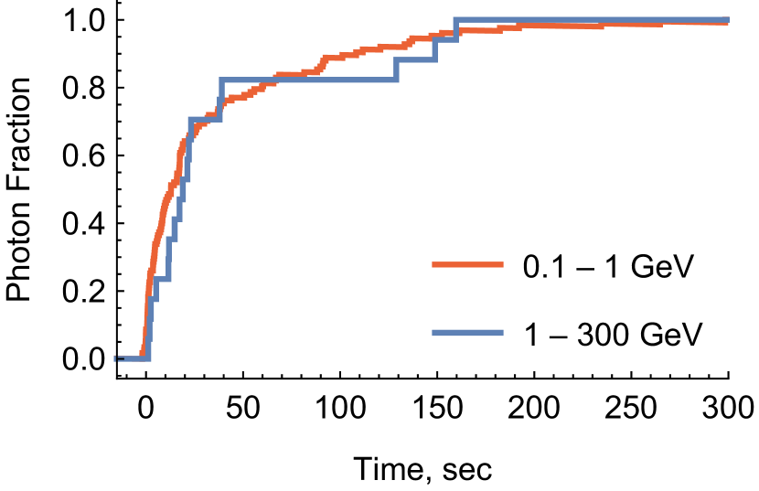
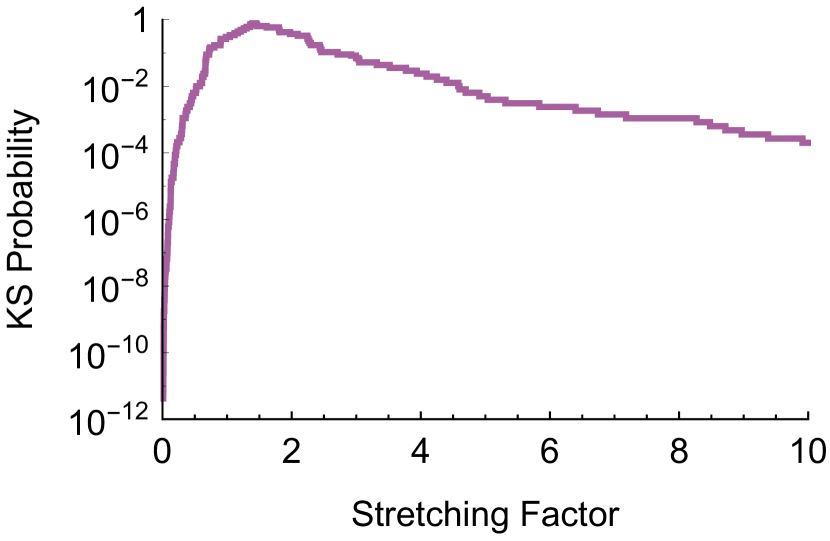
Figure 3: GRB 080916C light curves. Stretching factor is compatible with $\kappa=1$ within $2\sigma$.

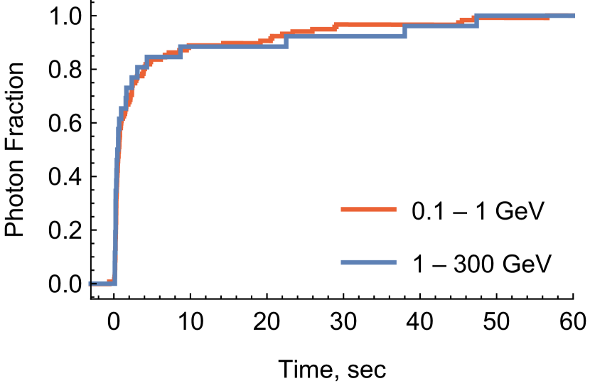
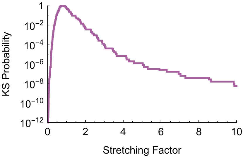
Figure 4: GRB 090510 light curves. Stretching factor is compatible with $\kappa=1$ within $1\sigma$.

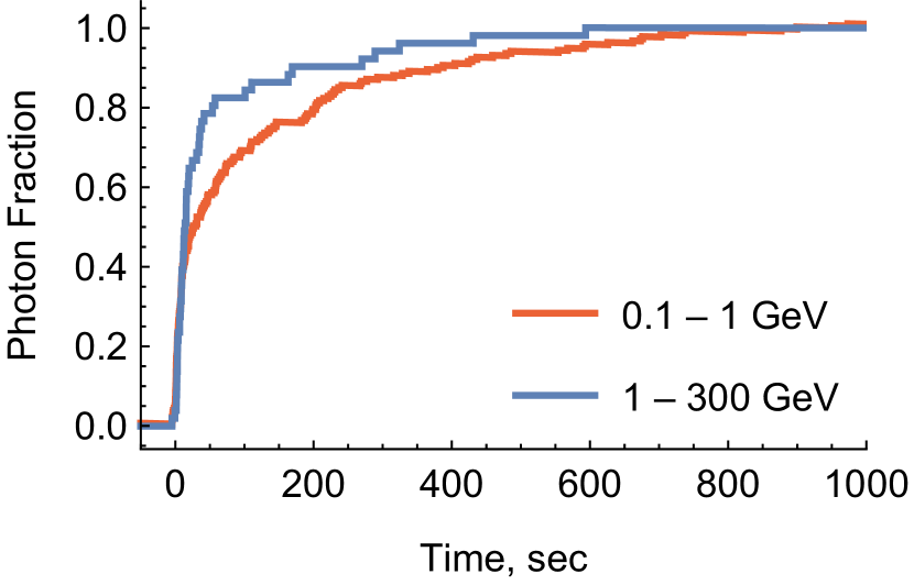
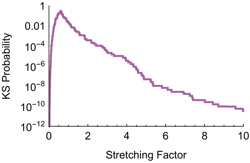
Figure 5: GRB 090902B light curves. Low energy radiation is stretched ($\kappa<1$) with significance of $2.3\sigma$.

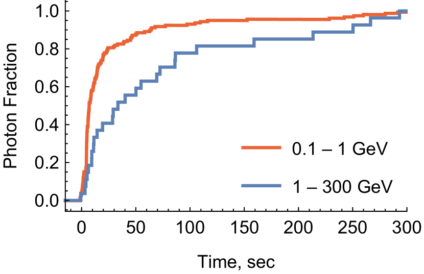
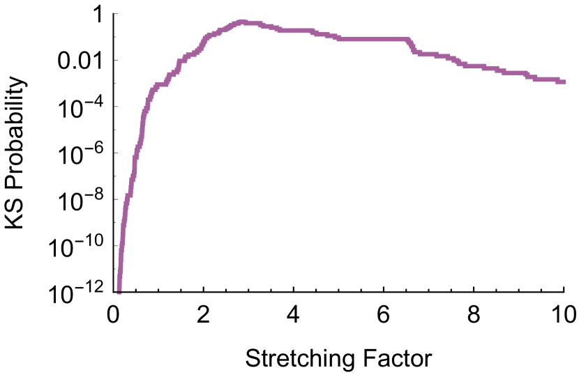
Figure 6: GRB 090926A light curves. High energy radiation is stretched ($\kappa>1$) with significance of $3.3\sigma$.

GRB	$1\sigma$		$2\sigma$		$3\sigma$		$4\sigma$		$5\sigma$
080916C	$1.04$  –	$2.24$	$0.67$  –	$3.32$	$0.42$  –	$5.83$	$0.19$  –	$14.9$	$0.087$  –	$35.7$
090501	$0.58$  –	$1.1$	$0.43$  –	$1.61$	$0.32$  –	$2.29$	$0.22$  –	$3.03$	$0.17$  –	$5.11$
090902B	$0.604$  –	$0.613$	$0.35$  –	$0.89$	$0.22$  –	$1.53$	$0.13$  –	$2.86$	$0.078$  –	$4.49$
090926A	$2.61$  –	$3.33$	$1.99$  –	$6.62$	$1.34$  –	$9.15$	$0.73$  –	$13.5$	$0.48$  –	$19.4$

Table 2: The ranges of allowed stretching factors for multiple levels of significance for the GRBs studied.

3 Model

The main idea behind our model is to assume that the burst opening angle depends on the energy of emitted photons, or, equivalently, that the most energetic plasma particles are concentrated near the axis of the jet, while low energy particles are on the periphery. As it’s seen in Figure 1 this leads to a time stretching effect due to relativistic beaming.

Although the details of the exact mechanism of the GRB are not known there are arguments in support of our model.

First of all, there are around 750 GRBs detected by GBM, half of which are in the LAT field of view at the moment of observation [1]. However, only about 30 of them were detected by the LAT, and only 4 of them were bright in the high energy band. If one extrapolates the uniform jet model to the very high energies, this observation would mean that these groups of bursts are internally different: some of them produce VHE radiation, while the others do not. These differences are hard to explain given that the burst energetics are similar [3]. These differences in burst counts find natural explanation in our model, in which the opening angle of a jet is inversely proportional to the energy of the photons it radiates. Therefore the most common scenario is that the off-axis angle of an observer is smaller than the low energy jet opening angle, but much larger than the opening angle of a high energy jet. Due to that, most of the bursts can only be seen at low energies. The 4 bursts we study in this paper were seen, according to our model, from the lowest off-axis angles.

Another argument comes from consideration of processes happening in jets, specifically the scattering of particles near the jet boundary. While plasma particles scatter, they simultaneously lose energy, and change directions, sometimes propagating beyond the jet boundary, and therefore increasing the jet opening angle. So, the processes of energy loss and increase of jet size are correlated, therefore the low energy particles should be closer to the jet boundary.

First, let us list the assumptions of the model:

1. Time $t=0$, a spherical shell of plasma is emitted. The center is called the central engine.

2. The shell points propagate with a constant velocity $v=\frac{\sqrt{\gamma^{2}-1}}{\gamma}\sim 1$, so at the time $t$ the radius of the shall is $vt$.

3. Each point of the shell is an isotropic radiator in its rest frame.

4. The radiation intensity is a function of the radiator position and the radiation frequency:

   $$\eta\left(r,\theta,\omega\right)=\frac{\eta_{0}}{1+\left(\frac{r}{r_{0}}\right)^{n}}\exp\left(-\left(\frac{\theta}{\theta_{0}}\right)^{2}\left(\frac{\omega}{\omega_{0}}\right)^{-2k}\right)\left(\frac{\omega}{\omega_{0}}\right)^{\alpha}$$ (2)

   $\eta$ is a number of particles emitted per volume per solid angle per frequency. It is a function of the distance $r$ from the central engine, of the off-axis angle $\theta$, and of the radiation frequency $\omega$.

The burst is fully defined by the following set of parameters:

• $\gamma$, the relativistic factor of the shell, $\gamma\gg 1$.

• $\eta_{0}$, which defines the luminosity scale.

• $r_{0}$, the characteristic jet length; $r_{0}\ll\frac{1}{H\left(0\right)}$, $H\left(t\right)$ is the Hubble parameter;

• $n$, which determines the sharpness of the jet end, $n>3$;

• $\omega_{0}$, a characteristic radiation frequency;

• $\theta_{0}$, the opening angle of the jet for radiation with frequency $\omega_{0}$, $\theta_{0}\ll 1$;

• $k$, which determines how much the opening angle changes with frequency, $k<0$;

• $\alpha$, the bare spectral index, $\alpha<-2k-1$

In the next step we calculate the observed light curves, and the stretching factors.

3.1 Photon observation time

We begin with computing a time at which some particular photon is observed. This time is a function of the radiator location $\left(r,\theta,\phi\right)$, as well as the observer location $\left(d,\chi,0\right)$ with respect to the burst center (we choose the coordinates so that the rotation angle of the observer is $0$.) We assume for now that the observer is too far from the jet to resolve its geometry, yet close enough so that the expansion of space is negligible. The latter assumption is made for simplicity of presentation. The cosmological expansion effect will be restored at the end of this section.

The observation time is a sum of two terms: the time interval from $t=0$ to the photon emission (the plasma time), and the time interval between the emission and the observation (the photon time):

$$t\left(r,\theta,\phi,d,\chi\right)=t_{\text{plasma}}\left(r\right)+t_{\text{photon}}\left(r,\theta,\phi,d,\chi\right)$$

$t_{\text{plasma}}$ is easy to compute since plasma moves with uniform velocity:

$$t_{\text{plasma}}\left(r\right)=\frac{r}{v}$$

$t_{\text{photon}}$ is a distance between the radiator and the observer:

$$t_{\text{photon}}\left(r,\theta,\phi,d,\chi\right) =\sqrt{\left(d\cos\chi-r\cos\theta\right)^{2}+\left(d\sin\chi-r\sin\theta\cos\phi\right)^{2}+\left(r\sin\theta\sin\phi\right)^{2}}$$

$$=d\sqrt{\left(\cos\chi-\frac{r}{d}\cos\theta\right)^{2}+\left(\sin\chi-\frac{r}{d}\sin\theta\cos\phi\right)^{2}+\left(\frac{r}{d}\sin\theta\sin\phi\right)^{2}}$$

$$\sim d\sqrt{\cos^{2}{\chi}-2\frac{r}{d}\cos\theta\cos\chi+\sin^{2}\chi-2\frac{r}{d}\sin\theta\cos\phi\sin\chi}$$

$$\sim d\left(1-\frac{r}{d}\left(\cos\theta\cos\chi+\sin\theta\cos\phi\sin\chi\right)\right)$$

$$=d-r\left(\cos\theta\cos\chi+\sin\theta\cos\phi\sin\chi\right)$$

Combining these expressions together, we get:

$$t\left(r,\theta,\phi,d,\chi\right)=d+r\left(\frac{1}{v}-\cos\theta\cos\chi-\sin\theta\cos\phi\sin\chi\right)$$

Since no photon can reach the observer faster than the speed of light, and the photons emitted at $t=0$ reach the observer at $t=d$, this time $t=d$ is the start of the observer’s light curve. So we can define a more convenient time origin:

$$\tau\left(r,\theta,\phi,\chi\right)=t\left(r,\theta,\phi,d,\chi\right)-d=r\left(\frac{1}{v}-\cos\theta\cos\chi-\sin\theta\cos\phi\sin\chi\right)$$

Finally, one can use the spherical law of cosines to write this in terms of the great-circle distance $\sigma\left(\theta,\phi,\chi\right)$ between the points $\left(\theta,\phi\right)$ and $\left(\chi,0\right)$:

$$\tau\left(r,\theta,\phi,\chi\right)=r\left(\frac{1}{v}-\cos\sigma\left(\theta,\phi,\chi\right)\right)$$ (3)

Note that $\tau$ doesn’t depend on $d$ anymore. But this is only true if we did not account for cosmology, or if the scale factor did not change from emission to observation. For a distant observer it will change, however, which will stretch the distances between photons:

$$\tau\left(r,\theta,\phi,z,\chi\right)=r\left(\frac{1}{v}-\cos\sigma\left(\theta,\phi,\chi\right)\right)\left(1+z\right)$$ (4)

Here $z$ is the redshift of the burst from the point of view of the observer.

3.2 Light curve

We now know enough to compute the observable quantity – the number of observed photons $p$. For that we need to integrate the radiation intensity $\eta$ over the four groups of variables. Two groups are burst-related: radiator position $\left(r,\theta,\phi\right)$ and frequency at emission $\omega^{\prime}$. The other two variables are related to observer: observation time $\tau$ and frequency at observation $\omega$. We relate the first two and the second two with the delta functions:

$$p\left(z,\chi;\tau_{1},\tau_{2};\omega_{1},\omega_{2}\right) =\frac{A_{\text{det}}}{A_{\text{ph}}\left(z\right)}\int_{0}^{\infty}\operatorname{d\!}r\int_{0}^{\pi}r\operatorname{d\!}\theta\int_{0}^{2\pi}r\sin{\theta}\operatorname{d\!}\phi\int_{0}^{\infty}\operatorname{d\!}\omega^{\prime}\int_{\tau_{1}}^{\tau_{2}}\operatorname{d\!}\tau\int_{\omega_{1}}^{\omega_{2}}\operatorname{d\!}\omega\,\eta\left(r,\theta,\omega^{\prime}\right)$$

$$\qquad{}\times\underbrace{\frac{1}{\gamma^{2}\left(1-v\cos\sigma\left(\theta,\phi,\chi\right)\right)^{2}}}_{\text{aberration}}\underbrace{\frac{1}{\gamma\left(1-v\cos\sigma\left(\theta,\phi,\chi\right)\right)}}_{\text{time dilation}}$$

$$\qquad{}\times\delta\left(\frac{\omega^{\prime}}{\underbrace{\gamma\left(1-v\cos\sigma\left(\theta,\phi,\chi\right)\right)}_{\text{relativistic shift}}\underbrace{\left(1+z\right)}_{\text{cosmological shift}}}-\omega\right)$$

$$\qquad{}\times\delta\left(\tau-r\left(\frac{1}{v}-\cos\sigma\left(\theta,\phi,\chi\right)\right)\left(1+z\right)\right)$$ (5)

Here $A_{\text{det}}$ is the effective area of the detector, and $A_{\text{ph}}$ is an area of the sphere over which photons emitted in the burst are spread (see appendix B for derivation). We have taken account for four relativistic effects, which affect intensities and frequencies of the radiators: relativistic aberration; time dilation of the radiators relative to the observer; relativistic blue/redshift; and cosmological redshift.

We integrate over $\omega^{\prime}$ and $r$ using the delta functions. For that we transform them as follows:

$$\delta\left(\frac{\omega^{\prime}}{\gamma\left(1-v\cos\sigma\right)\left(1+z\right)}-\omega\right) =\delta\left(\frac{1}{\gamma\left(1-v\cos\sigma\right)\left(1+z\right)}\left(\omega^{\prime}-\gamma\left(1-v\cos\sigma\right)\left(1+z\right)\omega\right)\right)$$

$$=\gamma\left(1-v\cos\sigma\right)\left(1+z\right)\delta\left(\omega^{\prime}-\gamma\left(1-v\cos\sigma\right)\left(1+z\right)\omega\right)$$

$$\delta\left(\tau-r\left(\frac{1}{v}-\cos\sigma\right)\left(1+z\right)\right) =\delta\left(\left(\frac{1}{v}-\cos\sigma\right)\left(1+z\right)\left(r-\frac{\tau}{\left(\frac{1}{v}-\cos\sigma\right)\left(1+z\right)}\right)\right)$$

$$=\frac{1}{\left(\frac{1}{v}-\cos\sigma\right)\left(1+z\right)}\delta\left(r-\frac{\tau}{\left(\frac{1}{v}-\cos\sigma\right)\left(1+z\right)}\right)$$

After the transformations expression for $p$ takes the following form:

$$p\left(z,\chi;\tau_{1},\tau_{2};\omega_{1},\omega_{2}\right) =\frac{A_{\text{det}}}{A_{\text{ph}}\left(z\right)}\int_{0}^{\pi}\operatorname{d\!}\theta\int_{0}^{2\pi}\operatorname{d\!}\phi\int_{\tau_{1}}^{\tau_{2}}\operatorname{d\!}\tau\int_{\omega_{1}}^{\omega_{2}}\operatorname{d\!}\omega$$

$$\qquad{}\times\eta\left(\frac{\tau}{\left(\frac{1}{v}-\cos\sigma\left(\theta,\phi,\chi\right)\right)\left(1+z\right)},\theta,\gamma\left(1-v\cos\sigma\left(\theta,\phi,\chi\right)\right)\left(1+z\right)\omega\right)$$

$$\qquad{}\times\frac{\tau^{2}\sin\theta}{\left(\frac{1}{v}-\cos\sigma\left(\theta,\phi,\chi\right)\right)^{3}\left(1+z\right)^{2}\gamma^{2}\left(1-v\cos\sigma\left(\theta,\phi,\chi\right)\right)^{2}}$$

$$=\frac{A_{\text{det}}}{A_{\text{ph}}\left(z\right)}\frac{1}{v^{2}\gamma^{2}\left(1+z\right)^{2}}\int_{\tau_{1}}^{\tau_{2}}\operatorname{d\!}\tau\,\tau^{2}\int_{0}^{\frac{\pi}{2}}\operatorname{d\!}\theta\int_{0}^{2\pi}\operatorname{d\!}\phi\int_{\omega_{1}}^{\omega_{2}}\operatorname{d\!}\omega\frac{\sin\theta}{\left(\frac{1}{v}-\cos\sigma\left(\theta,\phi,\chi\right)\right)^{5}}$$

$$\qquad{}\times\eta\left(\frac{\tau}{\left(\frac{1}{v}-\cos\sigma\left(\theta,\phi,\chi\right)\right)\left(1+z\right)},\theta,\gamma\left(1-v\cos\sigma\left(\theta,\phi,\chi\right)\right)\left(1+z\right)\omega\right)$$ (6)

Furthermore, one may integrate over $\omega$ and $\tau$ after using an explicit form for $\eta$ Eq. 2:

$$p\left(z,\chi;\tau_{1},\tau_{2};\omega_{1},\omega_{2}\right) =\frac{A_{\text{det}}}{A_{\text{ph}}\left(z\right)}\frac{1}{v^{2}\gamma^{2}\left(1+z\right)^{2}}\int_{0}^{\pi}\operatorname{d\!}\theta\int_{0}^{2\pi}\operatorname{d\!}\phi\int_{\omega_{1}}^{\omega_{2}}\operatorname{d\!}\omega\int_{\tau_{1}}^{\tau_{2}}\operatorname{d\!}\tau\,\tau^{2}\frac{\sin\theta}{\left(\frac{1}{v}-\cos\sigma\left(\theta,\phi,\chi\right)\right)^{5}}$$

$$\qquad{}\times\frac{\eta_{0}}{1+\left(\frac{\tau}{r_{0}\left(\frac{1}{v}-\cos\sigma\left(\theta,\phi,\chi\right)\right)\left(1+z\right)}\right)^{n}}$$

$$\qquad{}\times\exp\left(-\left(\frac{\theta}{\theta_{0}}\right)^{2}\left(\frac{\omega\gamma\left(1-v\cos\sigma\left(\theta,\phi,\chi\right)\right)\left(1+z\right)}{\omega_{0}}\right)^{-2k}\right)$$

$$\qquad{}\times\left(\frac{\omega\gamma\left(1-v\cos\sigma\left(\theta,\phi,\chi\right)\right)\left(1+z\right)}{\omega_{0}}\right)^{\alpha}$$

$$=\frac{A_{\text{det}}}{A_{\text{ph}}\left(z\right)}\frac{\eta_{0}}{\left(v\gamma\left(1+z\right)\right)^{2-\alpha}}\int_{0}^{\pi}\operatorname{d\!}\theta\int_{0}^{2\pi}\operatorname{d\!}\phi\frac{\sin\theta}{\left(\frac{1}{v}-\cos\sigma\left(\theta,\phi,\chi\right)\right)^{5-\alpha}}$$

$$\qquad{}\times\int_{\omega_{1}}^{\omega_{2}}\operatorname{d\!}\omega\exp\left(-\left(\frac{\theta}{\theta_{0}}\right)^{2}\left(\frac{\omega\gamma\left(1-v\cos\sigma\left(\theta,\phi,\chi\right)\right)\left(1+z\right)}{\omega_{0}}\right)^{-2k}\right)\left(\frac{\omega}{\omega_{0}}\right)^{\alpha}$$

$$\qquad{}\times\int_{\tau_{1}}^{\tau_{2}}\operatorname{d\!}\tau\,\tau^{2}\frac{1}{1+\left(\frac{\tau}{r_{0}\left(\frac{1}{v}-\cos\sigma\left(\theta,\phi,\chi\right)\right)\left(1+z\right)}\right)^{n}}$$

$$=\frac{A_{\text{det}}}{A_{\text{ph}}\left(z\right)}\frac{\eta_{0}}{\left(v\gamma\left(1+z\right)\right)^{2-\alpha}}\int_{0}^{\pi}\operatorname{d\!}\theta\int_{0}^{2\pi}\operatorname{d\!}\phi\frac{\sin\theta}{\left(\frac{1}{v}-\cos\sigma\left(\theta,\phi,\chi\right)\right)^{5-\alpha}}$$

$$\qquad{}\times\left(I\left(z,\chi,\omega_{2};\theta,\phi\right)-I\left(z,\chi,\omega_{1};\theta,\phi\right)\right)\left(J\left(z,\chi,\tau_{2};\theta,\phi\right)-J\left(z,\chi,\tau_{1};\theta,\phi\right)\right)$$ (7)

Here $I$ and $J$ are indefinite integrals over $\omega$ and $\tau$:

$$I\left(z,\chi,\omega;\theta,\phi\right) =\frac{\omega\left(\frac{\omega}{\omega_{0}}\right)^{\alpha}E_{\frac{\alpha+1}{2k}+1}\left(\left(\frac{\theta}{\theta_{0}}\right)^{2}\left(\frac{\omega}{\omega_{0}}\right)^{-2k}\left(\gamma\left(1-v\cos\sigma\left(\theta,\phi,\chi\right)\right)\left(1+z\right)\right)^{-2k}\right)}{2k}$$ (8)

$$J\left(z,\chi,\tau;\theta,\phi\right) =\frac{\tau^{3}}{3}\,_{2}F_{1}\left(1,\frac{3}{n};\frac{n+3}{n};-\left(\frac{\tau}{r_{0}\left(\frac{1}{v}-\cos\sigma\left(\theta,\phi,\chi\right)\right)\left(1+z\right)}\right)^{n}\right)$$ (9)

where exponential integral function $E_{n}\left(x\right)=\int_{1}^{\infty}\frac{e^{-xt}\operatorname{d\!}t}{t^{n}}$.

The remaining integrals over $\theta$ and $\chi$ are hard to do symbolically, so we compute them numerically. To optimize this computation we can use the assumption of small $\theta$ and $\chi$, so that:

$$\sin\theta \sim\theta$$

$$\cos\sigma\left(\theta,\phi,\chi\right) =\cos\theta\cos\chi+\sin\theta\sin\chi\cos\phi\sim 1-\frac{\theta^{2}}{2}-\frac{\chi^{2}}{2}+\theta\chi\cos\phi$$

Using this assumption, and the evenness of the integral as a function of $\theta$, we arrive to the optimized expressions for $p$, $I$ and $J$:

$$p\left(z,\chi;\tau_{1},\tau_{2};\omega_{1},\omega_{2}\right) =\frac{A_{\text{det}}}{A_{\text{ph}}\left(z\right)}\frac{2\eta_{0}}{\left(v\gamma\left(1+z\right)\right)^{2-\alpha}}\int_{0}^{\infty}\operatorname{d\!}\theta\int_{0}^{\pi}\operatorname{d\!}\phi\frac{\theta}{\left(\frac{1}{v}-1+\frac{\theta^{2}}{2}+\frac{\chi^{2}}{2}-\theta\chi\cos\phi\right)^{5-\alpha}}$$

$$\qquad{}\times\left(I\left(z,\chi,\omega_{2};\theta,\phi\right)-I\left(z,\chi,\omega_{1};\theta,\phi\right)\right)\left(J\left(z,\chi,\tau_{2};\theta,\phi\right)-J\left(z,\chi,\tau_{1};\theta,\phi\right)\right)$$ (10)

$$I\left(z,\chi,\omega;\theta,\phi\right) =\frac{\omega\left(\frac{\omega}{\omega_{0}}\right)^{\alpha}E_{\frac{\alpha+1}{2k}+1}\left(\left(\frac{\theta}{\theta_{0}}\right)^{2}\left(\frac{\omega}{\omega_{0}}\right)^{-2k}\left(v\gamma\left(1+z\right)\left(\frac{1}{v}-1+\frac{\theta^{2}}{2}+\frac{\chi^{2}}{2}-\theta\chi\cos\phi\right)\right)^{-2k}\right)}{2k}$$ (11)

$$J\left(z,\chi,\tau;\theta,\phi\right) =\frac{\tau^{3}}{3}\,_{2}F_{1}\left(1,\frac{3}{n};\frac{n+3}{n};-\left(\frac{\tau}{r_{0}\left(\frac{1}{v}-1+\frac{\theta^{2}}{2}+\frac{\chi^{2}}{2}-\theta\chi\cos\phi\right)\left(1+z\right)}\right)^{n}\right)$$ (12)

Finally, we need to compute the limits of $p$ for $\omega_{2}\rightarrow\infty$ and $\tau_{2}\rightarrow\infty$. It requires us to know the limit of $I$ for $\omega\rightarrow\infty$ (here we assume that $k<0$):

$$I\left(z,\chi,\infty;\theta,\phi\right)=\lim_{\omega\rightarrow\infty}I\left(z,\chi,\omega;\theta,\phi\right)=0$$ (13)

and the limit of $J$ for $\tau\rightarrow\infty$ ($n>3$ by assumption):

$$J\left(z,\chi,\infty;\theta,\phi\right)=\lim_{\tau\rightarrow\infty}J\left(z,\chi,\tau;\theta,\phi\right)=\left(r_{0}\left(\frac{1}{v}-1+\frac{\theta^{2}}{2}+\frac{\chi^{2}}{2}-\theta\chi\cos\phi\right)\left(1+z\right)\right)^{3}\frac{\pi}{n\sin\frac{3\pi}{n}}$$ (14)

The following quantities of phenomenological importance may be computed with the use of $p$:

• the total number of particles observed in a given energy range, $p_{\infty}\left(z,\chi;\omega_{1},\omega_{2}\right)=p\left(z,\chi;0,\infty;\omega_{1},\omega_{2}\right)$;

• the fraction of photons observed during a given time interval, $\Phi\left(z,\chi;\tau_{1},\tau_{2};\omega_{1},\omega_{2}\right)=\frac{p\left(z,\chi;\tau_{1},\tau_{2};\omega_{1},\omega_{2}\right)}{p_{\infty}\left(z,\chi;\omega_{1},\omega_{2}\right)}$;

• the duration of the burst $T_{f}\left(z,\chi;\omega_{1},\omega_{2}\right)$, that is the time by which the fraction $f$ of photons is observed. One may compute it by solving the following equation for $T_{f}$: $p\left(z,\chi;0,T_{f};\omega_{1},\omega_{2}\right)=fp_{\infty}\left(z,\chi;\omega_{1},\omega_{2}\right)$;

• the stretching factor, which will be discussed in the next section.

3.3 Stretching factor

The stretching factor for a continuous light curve is defined exactly like the stretching factor for a discrete one. It is the value of $\kappa$ which makes the KS-distance minimal:

$$\kappa\left(z,\chi;\omega_{1},\omega_{2},\omega_{3}\right)=\operatorname*{argmin}_{\kappa}\max_{\tau}\left|\Phi\left(z,\chi;0,\tau;\omega_{1},\omega_{2}\right)-\Phi\left(z,\chi;0,\kappa\tau;\omega_{2},\omega_{3}\right)\right|$$ (15)

The maximum of an absolute value is not differentiable, so the computation of $\kappa$ by the given definition is complicated. One may instead rewrite this expression in terms of a positive and a negative KS-distances:

$$D_{+}\left(z,\chi;\kappa;\omega_{1},\omega_{2},\omega_{3}\right) =\max_{\tau}\left(\Phi\left(z,\chi;0,\tau;\omega_{1},\omega_{2}\right)-\Phi\left(z,\chi;0,\kappa\tau;\omega_{2},\omega_{3}\right)\right)$$

$$D_{-}\left(z,\chi;\kappa;\omega_{1},\omega_{2},\omega_{3}\right) =\min_{\tau}\left(\Phi\left(z,\chi;0,\tau;\omega_{1},\omega_{2}\right)-\Phi\left(z,\chi;0,\kappa\tau;\omega_{2},\omega_{3}\right)\right)$$

$$\kappa\left(z,\chi;\omega_{1},\omega_{2},\omega_{3}\right) =\operatorname*{argmin}_{\kappa}\max\left(D_{+}\left(z,\chi;\kappa;\omega_{1},\omega_{2},\omega_{3}\right),-D_{-}\left(z,\chi;\kappa;\omega_{1},\omega_{2},\omega_{3}\right)\right)$$

Take note that $\Phi$ monotonously increases with $\tau$. It implies that $D_{+}$ and $D_{-}$ monotonously decrease with $\kappa$, so as $D_{+}+D_{-}$. So there is a single value of $\kappa$, for which

$$D_{+}\left(z,\chi;\kappa;\omega_{1},\omega_{2},\omega_{3}\right)=-D_{-}\left(z,\chi;\kappa;\omega_{1},\omega_{2},\omega_{3}\right)$$ (16)

And this value of $\kappa$ also makes the $\max\left({D_{+},-D_{-}}\right)$ minimal, since $D_{+}$ monotonously decrease, and $\left(-D_{-}\right)$ monotonously increase with $\kappa$.

So we arrive at a simpler way to compute $\kappa$ by solving an equation instead of computing the minimum.

Being able to compute the stretching factor, we could now compare our model predictions with observations given the position of an observer. We don’t know the observer’s off-axis angle $\chi$, however, so we cannot check the stretching factor prediction on the burst-to-burst basis. Instead, we focus on a series of tests, which will ensure that our model doesn’t contradict to existing observations. Namely the test of the total energy and comparison with Fermi-LAT data of the distribution of the stretching factors and the fraction of the high-energy bursts. These tests will be discussed in the following section.

4 Observational tests

4.1 Total energy

In the first test we compute the total energy radiated from the burst, and ensure that it doesn’t exceed the mass of the star from which the burst originated.

To compute the total energy, we need to multiply the radiation intensity by frequency, and integrate it over frequencies $\omega$, volume $\left(r,\theta,\phi\right)$, and observer positions $\left(\sigma,\xi\right)$. We assume $\theta\ll 1$, and have taken into account the same relativistic effects as we did in the observed particle count computation:

$$E =\int_{0}^{\infty}\operatorname{d\!}\omega\int_{0}^{\infty}\operatorname{d\!}r\int_{0}^{\infty}r\operatorname{d\!}\theta\int_{0}^{2\pi}r\,\theta\operatorname{d\!}\phi\int_{0}^{\infty}\operatorname{d\!}\sigma\int_{0}^{2\pi}\sin\sigma\operatorname{d\!}\xi$$

$$\quad{}\times\eta\left(r,\theta,\omega\right)\underbrace{\frac{1}{\gamma\left(1-v\cos\sigma\right)}}_{\text{time dilation}}\underbrace{\frac{1}{\gamma^{2}\left(1-v\cos\sigma\right)^{2}}}_{\text{aberration}}\underbrace{\frac{\omega}{\gamma\left(1-v\cos\sigma\right)}}_{\text{relativistic shift}}$$ (17)

$$=\frac{4\pi^{2}}{\gamma^{4}}\int_{0}^{\infty}\operatorname{d\!}\omega\,\omega\int_{0}^{\infty}\operatorname{d\!}r\,r^{2}\int_{0}^{\infty}\operatorname{d\!}\theta\,\theta\,\eta\left(r,\theta,\omega\right)\int_{0}^{\infty}\operatorname{d\!}\sigma\frac{\sin\sigma}{\left(1-v\cos\sigma\right)^{4}}$$

An integral over $\sigma$ is computable analytically:

$$\int_{0}^{\infty}\operatorname{d\!}\sigma\frac{\sin\sigma}{\left(1-v\cos\sigma\right)^{4}}=\frac{2\left(3+v^{2}\right)}{3\left(1-v^{2}\right)^{3}}=\frac{2}{3}\gamma^{6}\left(4-\frac{1}{\gamma^{2}}\right)$$

Substituting this result into the expression for $E$ we get:

$$E=\frac{32\pi^{2}}{3}\left(\gamma^{2}-\frac{1}{4}\right)\int_{0}^{\infty}\operatorname{d\!}\omega\,\omega\int_{0}^{\infty}\operatorname{d\!}r\,r^{2}\int_{0}^{\infty}\operatorname{d\!}\theta\,\theta\,\eta\left(r,\theta,\omega\right)$$ (18)

Now we can use the expression for $\eta$ to do the remaining integrals:

$$E=\frac{32\pi^{2}\eta_{0}}{3}\left(\gamma^{2}-\frac{1}{4}\right)\int_{0}^{\infty}\operatorname{d\!}\omega\,\omega\left(\frac{\omega}{\omega_{0}}\right)^{\alpha}\int_{0}^{\infty}\operatorname{d\!}r\,\frac{r^{2}}{1+\left(\frac{r}{r_{0}}\right)^{n}}\int_{0}^{\infty}\operatorname{d\!}\theta\,\theta\,\exp\left(-\left(\frac{\theta}{\theta_{0}}\right)^{2}\left(\frac{\omega}{\omega_{0}}\right)^{-2k}\right)$$

The integrals over $r$ and $\theta$ can be computed symbolically:

$$\int_{0}^{\infty}\operatorname{d\!}r\,\frac{r^{2}}{1+\left(\frac{r}{r_{0}}\right)^{n}}=\frac{\pi}{n\sin\left(\frac{3\pi}{n}\right)}r_{0}^{3}$$

$$\int_{0}^{\infty}\operatorname{d\!}\theta\,\theta\,\exp\left(-\left(\frac{\theta}{\theta_{0}}\right)^{2}\left(\frac{\omega}{\omega_{0}}\right)^{-2k}\right)=\frac{1}{2}\theta_{0}^{2}\left(\frac{\omega}{\omega_{0}}\right)^{2k}$$

Now we have only one integral left:

$$E=\frac{16\pi^{3}}{3n\sin\left(\frac{3\pi}{n}\right)}\left(\gamma^{2}-\frac{1}{4}\right)\,\eta_{0}\,r_{0}^{3}\,\theta_{0}^{2}\int_{0}^{\infty}\operatorname{d\!}\omega\,\omega\left(\frac{\omega}{\omega_{0}}\right)^{2k+\alpha}$$ (19)

Note, however, that since $\alpha<-2k-1$ this integral diverges for $\omega\rightarrow 0$. This is not a problem as long as our model is not expected to describe low-energy radiation of the burst. One should ensure that the total energy of the high-energy radiation is not too large. For this test, we integrate only over those radiators which emission is observed by Fermi LAT, that is over the frequencies greater than $\frac{\omega_{1}}{\gamma}$, where $\omega_{1}$ is the smallest observable photon frequency. Now we compute the last integral and get the final expression for $E$:

$$E\left(\omega_{1}\right) =\frac{16\pi^{3}}{3n\sin\left(\frac{3\pi}{n}\right)}\left(\gamma^{2}-\frac{1}{4}\right)\,\eta_{0}\,r_{0}^{3}\,\theta_{0}^{2}\int_{\frac{\omega_{1}}{\gamma}}^{\infty}\operatorname{d\!}\omega\,\omega\left(\frac{\omega}{\omega_{0}}\right)^{2k+\alpha}$$

$$=\frac{16\pi^{3}}{3n\sin\left(\frac{3\pi}{n}\right)}\left(\gamma^{2}-\frac{1}{4}\right)\,\eta_{0}\,r_{0}^{3}\,\theta_{0}^{2}\frac{\omega_{1}^{2}\left(\frac{\omega_{1}}{\gamma\omega_{0}}\right)^{2k+\alpha}}{\gamma^{2}(-2k-\alpha-2)}$$

$$=\frac{16\pi^{3}}{3n\left(-2k-\alpha-2\right)\sin\left(\frac{3\pi}{n}\right)}\gamma^{-2k-\alpha}\left(1-\frac{1}{4\gamma^{2}}\right)\,\eta_{0}\,r_{0}^{3}\,\theta_{0}^{2}\frac{\omega_{0}^{-2k-\alpha}}{\omega_{1}^{-2k-\alpha-2}}$$ (20)

This energy should not exceed a typical mass $M_{s}$ of a massive star. So, finally, we arrive at the first constraint for the burst parameters:

$$\frac{16\pi^{3}}{3n\left(-2k-\alpha-2\right)\sin\left(\frac{3\pi}{n}\right)}\gamma^{-2k-\alpha}\left(1-\frac{1}{4\gamma^{2}}\right)\,\eta_{0}\,r_{0}^{3}\,\theta_{0}^{2}\frac{\omega_{0}^{-2k-\alpha}}{\omega_{1}^{-2k-\alpha-2}}<M_{s}$$ (21)

4.2 Distribution of stretching factors

The second test is to calculate the distribution of stretching factors of observable bursts, and to compare it to observations.

The computation of the exact and precise distribution is technically hard and computationally intensive because stretching factor is not a monotonic function of neither redshift nor off-axis angles. We do not compute the distribution directly. Instead, we use the Monte-Carlo method to produce a large representative sample of stretching factors. Then, we calculate an empirical CDF of this sample, which can be compared with observations using the KS-test. Since one may compute much larger sample than that of observations, there is no precision loss due to this simplification.

We still have one ingredient missing though – the evolution of the bursts density. We assume that the bursts density is roughly proportional to the stars density, and the latter is roughly proportional to the matter density, which changes with $z$ as $\left(1+z\right)^{3}$. It is clear, however, that since no stars existed at very small redshifts, the burst density should decline there, so we add an exponential cutoff to it:

$$\rho=\rho_{0}\left(1+z\right)^{3}\exp\left(-\frac{z}{z_{c}}\right)\,$$ (22)

where $\rho_{0}$ is a normalization factor, and $z_{c}$ is a redshift scale, after which the density is cut off.

For the modeling we first need to define the range of redshifts and off-axis angles. The range should include all the observable jet positions, but one should keep the range as small as possible in order to avoid production of too many points corresponding to invisible bursts. For simplicity we consider the rectangular region.

We start with selecting a range for redshifts. Ideally, one would expect that this range starts with $z=0$. Then, however, there will be visible jets for all possible off-axis angles, which will make our angles range too large. Note also, that since the bursts count increases with redshift as $z^{3}$, the probability to observe a low-redshift burst is very small. So instead of selecting the smallest redshift to be $0$, we select it to be a small number $z_{\text{min}}=0.1$.

$z_{\text{max}}$ is defined by the farthest jet, which can be observed. Since the burst observability $p_{\infty}\left(z,\chi;\omega_{2},\omega_{3}\right)$ decreases with both redshift and $\chi$, we can find the maximum redshift by solving the following equation:

$$p_{\infty}\left(z_{\text{max}},0;\omega_{2},\omega_{3}\right)=p_{\text{min}}\,,$$ (23)

where $p_{\text{min}}$ is the minimum number of particles required to claim an observation.

The observability declines with $z$ and $\chi$, so the observable burst with the largest $\chi$ should be located at the redshift $z_{\text{min}}$. We can find this angle by solving the similar equation, as we did for the redshifts:

$$p_{\infty}\left(z_{\text{min}},\chi_{\text{max}};\omega_{2},\omega_{3}\right)=p_{\text{min}}$$ (24)

The simulation is performed by repetition of the following 3 steps before the required number of bursts is attained:

1. First, the random redshift is generated following the distribution 22. This may be done with the Inverse transform sampling method. The CDF of the distribution of redshifts is a ratio of redshift counts in different space volumes:

   $$\Phi_{z}\left(z\right)=\frac{\int_{z_{\text{min}}}^{z}\rho\left(z^{\prime}\right)\operatorname{d\!}V\left(z^{\prime}\right)}{\int_{z_{\text{max}}}^{z_{\text{max}}}\rho\left(z^{\prime}\right)\operatorname{d\!}V\left(z^{\prime}\right)}$$ (25)

   where $\operatorname{d\!}V\left(z^{\prime}\right)$ is the volume of the infinitesimal shell surrounding a sphere over which bursts at redshift $z^{\prime}$ are distributed (see appendix B for derivation).

   To generate a redshift, one should uniformly select a value of $\Phi_{z}$, and solve the corresponding equation for $z$:

   $$\Phi_{z}\left(z\right)=x$$ (26)

   where $x$ is a random variable uniformly distributed in the range $0$ to $1$.

2. The random off-axis angle may be then generated with a similar method. The CDF of the angles distribution is a ratio of spherical areas:

   $$\Phi_{\chi}\left(\chi\right)=\frac{\int_{0}^{\chi}\sin\chi^{\prime}\operatorname{d\!}\chi^{\prime}}{\int_{0}^{\chi_{\text{max}}}\sin\chi^{\prime}\operatorname{d\!}\chi^{\prime}}\approx\frac{\int_{0}^{\chi}\chi^{\prime}\operatorname{d\!}\chi^{\prime}}{\int_{0}^{\chi_{\text{max}}}\chi^{\prime}\operatorname{d\!}\chi^{\prime}}=\left(\frac{\chi}{\chi_{\text{max}}}\right)^{2}\,.$$ (27)

   As with redshifts, we get a properly distributed $\chi$ by solving the equation:

   $$\Phi_{\chi}\left(\chi\right)=\left(\frac{\chi}{\chi_{\text{max}}}\right)^{2}=y\,,$$ (28)

   $$\chi=\chi_{\text{max}}\sqrt{y}\,,$$ (29)

   where $y$ is an another independent random variable uniformly distributed in the range $0$ to $1$.

3. Now we check, whether the burst in a selected position may be observed: $p_{\infty}\left(z,\chi;\omega_{2},\omega_{3}\right)>p_{\text{min}}$. If it is, add $\kappa\left(z,\chi\right)$ to the sample.

With this algorithm, we arrive to the stretching factor distribution which may be compared with the observed one.

4.3 High energy bursts fraction

Our final test is based on the answer to the following question: given the bursts observed in the whole energy range $\left(\omega_{1},\omega_{3}\right)$, which fraction of them may also be observed in the high energy range $\left(\omega_{2},\omega_{3}\right)$?

To calculate this ratio, one needs to compute the number of bursts visible in a given energy range, which is the integral over space and jet directions:

$$b\left(\omega_{1},\omega_{2}\right) =\int_{0}^{z_{\text{max}}\left(\omega_{1},\omega_{2}\right)}\operatorname{d\!}V\left(z\right)\rho\left(z\right)\int_{0}^{\chi_{\text{max}}\left(z,\omega_{1},\omega_{2}\right)}2\pi\sin\chi\operatorname{d\!}\chi$$

$$\approx 2\pi\int_{0}^{z_{\text{max}}\left(\omega_{1},\omega_{2}\right)}\operatorname{d\!}V\left(z\right)\rho\left(z\right)\int_{0}^{\chi_{\text{max}}\left(z,\omega_{1},\omega_{2}\right)}\chi\operatorname{d\!}\chi=\pi\int_{0}^{z_{\text{max}}\left(\omega_{1},\omega_{2}\right)}\operatorname{d\!}V\left(z\right)\rho\left(z\right)\chi^{2}_{\text{max}}\left(z,\omega_{1},\omega_{2}\right)\,,$$ (30)

where $z_{\text{max}}\left(\omega_{1},\omega_{2}\right)$ and $\chi_{\text{max}}\left(z,\omega_{1},\omega_{2}\right)$ are the same values we used in the previous section: the maximum redshift from which a burst can be observed in a given energy range, and the maximum off-axis angle with which the burst at redshift $z$ can be observed.

The required fraction is the ratio of these integrals:

$$f\left(\omega_{1},\omega_{2},\omega_{3}\right)=\frac{b\left(\omega_{2},\omega_{3}\right)}{b\left(\omega_{1},\omega_{3}\right)}=\frac{\int_{0}^{z_{\text{max}}\left(\omega_{2},\omega_{3}\right)}\operatorname{d\!}V\left(z\right)\rho\left(z\right)\chi^{2}_{\text{max}}\left(z,\omega_{2},\omega_{3}\right)}{\int_{0}^{z_{\text{max}}\left(\omega_{1},\omega_{3}\right)}\operatorname{d\!}V\left(z\right)\rho\left(z\right)\chi^{2}_{\text{max}}\left(z,\omega_{1},\omega_{3}\right)}\,.$$ (31)

Our 3rd test is the comparison of the obtained ratio with the observed value.

5 Results

5.1 Parameter fit

For now we have discussed how to compute various observables of the model, and how to test the model against the data from observations. Now we come to the discussion of specific values for the parameters of the burst.

First of all, we need to determine, which parameters to fit. At most, the observables of a particular burst depend on 10 parameters: 8 of the burst $\left(\gamma,\eta_{0},r_{0},n,\omega_{0},\theta_{0},k,\alpha\right)$, and 2 of the observer’s position related to the burst $\left(z,\chi\right)$. However, some of these parameters only change observables trivially, and, also, there are transformations of variables, which do not change observables at all (see equation 3.2):

• The number of photons $p$ depends linearly on $\eta_{0}$, so $\eta_{0}$ doesn’t affect other observables like duration, or stretching factor. One can easily fit $\eta_{0}$ to match the observed photon count.

• If we make a simultaneous transformation of $r_{0}\rightarrow\lambda r_{0}$ and $\eta_{0}\rightarrow\frac{1}{\lambda^{3}}\eta_{0}$, where $\lambda$ is a parameter of transformation, only duration of the burst will change. Other observables, like the total number of photons, or stretching factor, will not be affected.

• Finally, if we make a following transformation: $\omega_{0}\rightarrow\lambda\omega_{0}$, $\theta_{0}\rightarrow\lambda^{k}\theta_{0}$, $\eta_{0}\rightarrow\lambda^{\alpha}\eta_{0}$, where $\lambda$ is another transformation parameter, no observables will change whatsoever.

Given these transformations, one can reduce the number of parameters for fit to 7: $\left(\gamma,n,\theta_{0},k,\alpha,z,\chi\right)$.

Also, some of these parameters are known from observations:

• Redshifts $z$ of many bursts have been measured [10].

• We know that relativistic factors $\gamma$ are on the order of magnitude of $\gamma=300$ [19].

This knowledge allows us to reduce the number of parameters to minimize against to just 5: $\left(n,\theta_{0},k,\alpha,\chi\right)$.

The best fit parameters are found by minimizing the cost function $C\left(n,\theta_{0},k,\alpha,\chi\right)$ which should satisfy the following objectives:

• Total energy of the burst is finite (that is $k+\frac{\alpha}{2}+1<0$) and smaller than $6\times 10^{53}\,\mathrm{GeV}\approx 10^{51}\,\mathrm{erg}$ [2].

• The stretching factor of the burst should be compatible with the value for the GRB 090926A.

• The ratio of photons with high energies and low energies should be compatible with the value for the GRB 090926A, $\frac{p_{\infty}\left(z,\chi;1\,\mathrm{GeV},\infty\right)}{p_{\infty}\left(z,\chi;0.1\,\mathrm{GeV},1\,\mathrm{GeV}\right)}=0.057$.

• The burst should not be too faint compared to other bursts from the sample. In other words, the total number of observed photons should approximately equal to the median among the sample.

• We assume that all bursts have the same burst parameters $\left(\gamma,\eta_{0},r_{0},n,\omega_{0},\theta_{0},k,\alpha\right)$ and require that bursts with small stretching factors like GRB 090902B should be possible to observe. So we require that bursts with the stretching factor of GRB 090902B or lower appear in random samples by varying $z$ and $\chi$ (sampling is done the same way as in Section 4.2). Note that this requirement unlike others applies to an ensemble of simulated bursts.

The cost function is then computed by the following procedure:

1. Set $\gamma=300$, $\omega_{0}=1\,\mathrm{GeV}$, $z=2.1062$ (which is the redshift of GRB 090926A)

2. Set $\eta_{0}$ and $r_{0}$ such that the duration of the burst, and the total number of observed photons are compatible with GRB 090926A, $T_{0.99}\left(z,\chi;0.1\,\mathrm{GeV},\infty\right)=219.5\,\mathrm{sec}$ and $p_{\infty}\left(z,\chi;0.1\,\mathrm{GeV},\infty\right)=179.996$

3. If $k+\frac{\alpha}{2}+1<0$, or the energy of the burst $E\left(0.1\,\mathrm{GeV}\right)>6\times 10^{53}\,\mathrm{GeV}$, the cost function equals to the penalization factor: $C\left(n,\theta_{0},k,\alpha,\chi\right)=400$.

4. Compute the small sample of 10 bursts (we will need stretching factors and total photon counts) with the same fixed burst parameters $\left(\gamma,\eta_{0},r_{0},n,\omega_{0},\theta_{0},k,\alpha\right)$, and with $z$ and $\chi$ representatively distributed (as discussed in Section 4.2).

5. Compute the cost due to the stretching factor:

   $$C_{\kappa}=\frac{\log{\kappa\left(z,\chi;0.1\,\mathrm{GeV},1\,\mathrm{GeV},\infty\right)}-\log{\kappa_{\text{GRB090926A}}}}{\Delta\log\kappa_{\text{GRB090926A}}}$$ (32)

   Here $\log\kappa_{\text{GRB090926A}}=\frac{1}{2}\left(\log\left(6.62\right)+\log\left(1.99\right)\right)$ and $\Delta\log\kappa_{\text{GRB090926A}}=\frac{1}{2}\left(\log\left(6.62\right)-\log\left(1.99\right)\right)$.

6. Compute the cost due to the fraction of high and low energy photon counts:

   $$C_{f}=\frac{\log{\frac{p_{\infty}\left(z,\chi;1\,\mathrm{GeV},\infty\right)}{p_{\infty}\left(z,\chi;0.1\,\mathrm{GeV},1\,\mathrm{GeV}\right)}}-\log f_{\text{GRB090926A}}}{\log(10)}$$ (33)

   Here $f_{\text{GRB090926A}}=0.0570003$.

7. Compute the cost due to the brightness of the burst compared to the median:

   $$C_{b}=\frac{\log{\frac{p_{\infty}\left(z,\chi;0.1\,\mathrm{GeV},\infty\right)}{p_{\text{med}}}}-0}{\log(10)}$$ (34)

   Here $p_{\text{med}}$ is the median number of observed photons among the sample computed in the step 4.

8. Compute the cost due to the minimal stretching factor from the sample:

   $$C_{\kappa\text{min}}=\max\left(0,\frac{\log{\kappa_{\text{min}}}-\log{\kappa_{\text{GRB090902B}}}}{\Delta\log\kappa_{\text{GRB090902B}}}\right)$$ (35)

   Here $\kappa_{\text{min}}$ is the minimal stretching factor from the sample computed in the step 4, $\log\kappa_{\text{GRB090902B}}=\frac{1}{2}\left(\log\left(0.89\right)+\log\left(0.35\right)\right)$ and $\Delta\log\kappa_{\text{GRB090902B}}=\frac{1}{2}\left(\log\left(0.89\right)-\log\left(0.35\right)\right)$.

9. Finally, the value of the cost function is the sum of squares of the four:

   $$C=C_{\kappa}^{2}+C_{f}^{2}+C_{b}^{2}+C_{\kappa\text{min}}^{2}$$ (36)

$\mathrm{n}$	$\mathrm{\theta_{0}}$	$\mathrm{k}$	$\mathrm{\alpha}$	$\mathrm{\chi}$
$22.1525$	$\mathrm{2.16424\times 10^{-4}}$	$-0.417\,021$	$-1.351\,630\,0$	$\mathrm{7.04982\times 10^{-3}}$
$25.8640$	$\mathrm{4.90222\times 10^{-8}}$	$-2.908\,750$	$3.538\,010\,0$	$\mathrm{2.86570\times 10^{-4}}$
$17.5380$	$\mathrm{1.46284\times 10^{-3}}$	$-2.133\,600$	$-2.133\,600\,0$	$\mathrm{1.52624\times 10^{-3}}$
$17.9736$	$\mathrm{4.52631\times 10^{-6}}$	$-1.402\,620$	$-0.011\,413\,2$	$\mathrm{3.25900\times 10^{-4}}$
$5.0000$	$\mathrm{1.12535\times 10^{-7}}$	$-0.200\,000$	$-2.000\,000\,0$	$\mathrm{4.73795\times 10^{-3}}$
$7.0000$	$\mathrm{2.00000\times 10^{-12}}$	$-3.000\,000$	$-3.000\,000\,0$	$\mathrm{1.73795\times 10^{-3}}$

Table 3: Initial points used for minimization procedure from Section 5.1.

We use the Nelder-Mead (downhill simplex) method for the minimization procedure. Initial points were chosen to include the areas in parameter space where each cost is close to $0$ (first $4$ points correspondingly), and to cover the large fraction of the parameter space. You can see the values in Table 3.

The minimization converged to the following parameter values:

• $\gamma=300$

• $\eta_{0}=4.629640817921788\times 10^{34}\,\mathrm{sec^{-3}GeV^{-1}}$

• $r_{0}=3.142715108207946\times 10^{6}\,\mathrm{sec}$

• $\bm{n=22.9977}$

• $\omega_{0}=1\,\mathrm{GeV}$

• $\bm{\theta_{0}=7.93393\times 10^{-5}}$

• $\bm{k=-0.65356}$

• $\bm{\alpha=-0.724394}$

• $z=2.1062$

• $\bm{\chi=0.00590163}$

Note, that these parameter values (except for $z$ and $\chi$) are universal, and they may describe the whole population of observed bursts, as will be shown in the next section.

5.2 Results of the tests

As was discussed in the previous section our model can reproduce both stretching factors smaller than $1$ (like of GRB 090902B) and larger than $1$ (like of GRB 090926A) depending on redshift and observer’s off-axis angle (see fig. 2).

Below are the results of the tests of Section 4:

• The total energy emitted in $100\,\mathrm{MeV}$ and more energetic gamma rays $E<5.89\times 10^{53}\,\mathrm{GeV}$, which is in agreement with [2].

• The distribution of observable bursts’ stretching factors is shown in Fig. 7. This distribution does not contradict to the values of stretching factors obtained in Section 2.

• The fraction of bursts observable in low energy band, which are also observed in high energy band is $f_{m}=0.110$. The Fermi-LAT catalog contains $35$ bursts out of which $4$ can be observed in high energy band. Therefore the observed value $f_{o}=0.11\pm 0.05$ (error from binomial distribution) agrees with the model.

Therefore the model successfully explains the variety of the stretching factors observed by the Fermi LAT.

6 Discussion

The are some caveats and possible directions of improvement of the model. First of all, as it’s seen in Fig. 8 the stretching factor of GRB 090926A is higher that the model prediction. More data are needed to understand whether this requires a refinement of the model or is a statistical fluctuation.

Second, the shapes of light curves produced by the model (see fig. 2) differ considerably from observed ones (e.g. fig. 5). In particular, the slope of light curves produced by the model is zero at $t=0$, while the slope of the observed light curves at $t=0$ appears to have a maximum.

Third, the assumption of plasma energy dependence on off-axis angle should be better justified. This might probably be done using hydrodynamic simulation of the jet.

We note, that even though it appears that bursts are similar in their rest frames, this may be considered only as a first approximation. The differences in masses, metallicities, angular momenta of progenitor stars, and the differences in local conditions around them might account for differences in light curves of GRBs (or, even, for especially large stretching factor of GRB 090926A). This means that the minor variations of the model parameters might be necessary.

It seems, however, that all the issues above may be addressed by refining the model without changing it’s main assumptions.

Our study can be summarized with 3 main conclusions.

First, the time stretching of GRB light curves between different VHE (in particular $100\,\mathrm{MeV}<E<1\,\mathrm{GeV}$ and $E>1\,\mathrm{GeV}$) bands is discovered with the statistical significance of $3.3\sigma$. Depending on the burst the stretching factor may be higher or lower than 1, that is the higher or the lower-energy light curve is stretched.

Second, the time stretching may be explained with curvature effects, that is the effects of jet geometry. There is no need to introduce any new spectral components.

Finally, one may assume that all GRBs are the same in their rest frames. The internal burst parameters (such as $\gamma$, $\eta_{0}$, $r_{0}$, $n$, $\omega_{0}$, $\theta_{0}$, $k$ and $\alpha$) might stay the same for all bursts, and this assumption is more or less consistent with existing observations.

We note, that the model predicts a correlation between the fraction of the high energy photons, the stretching factor and the observer’s off-axis angle (see fig. 8). This may be used as a method to estimate the observer’s off-axis angle.

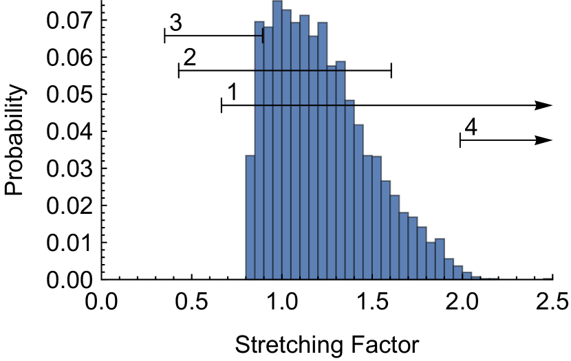
(a) Histogram (blue) obtained from the model. Black error bars show observed stretching factors.

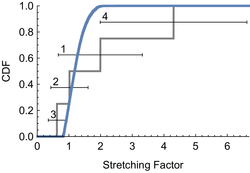
(b) CDF (blue) obtained from the model. Gray curve and black error bars show observed stretching factors.

Figure 7: Stretching factors histogram and CDF produced by our model. The sample contains $4096$ bursts. Numbered error bars correspond to GRB 080916C, GRB 090510, GRB 090902B and GRB 090926A (in this order).

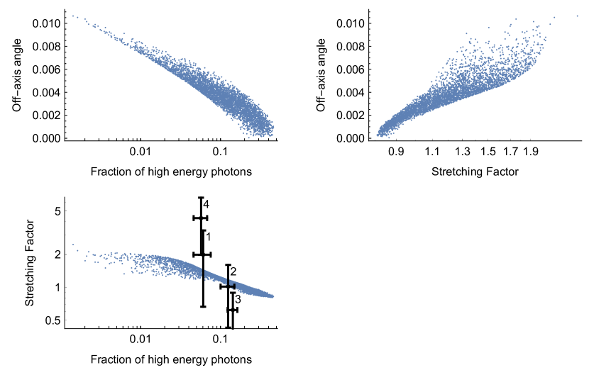
Figure 8: Correlations between off-axis angles, stretching factors and high to low energy photon count ratios found in the sample produced by our model. The sample contains $4096$ bursts. Numbered black crosses show data for GRB 080916C, GRB 090510, GRB 090902B and GRB 090926A (in this order) with $2\sigma$ error bars. This correlation allows one to estimate off-axis angles of observed bursts.

Acknowledgments. We thank A. Gruzinov, M. Pshirkov and S. Troitsky for comments and inspiring discussions. The work was supported by Russian Science Foundation grant 14-12-01340. The analysis is based on data and software provided by the Fermi Science Support Center (FSSC). The numerical part of the work was done at the cluster of the Theoretical Division of INR RAS. G.R. acknowledges the fellowship of the Dynasty foundation.

Appendix A Details of using Fermi Science tools

This appendix contains the details on using the Fermi-LAT data. Namely, the exact values passed to the web form on the Fermi-LAT data server and the code used to run the Fermi tools including the full list of options.

Parameters that are passed to the web form of the Fermi-LAT data server to download the bursts data are the following:

• Object name or coordinates. Coordinates are filled from the Table 1.

• Coordinate system. J2000.

• Search radius (degrees). $60$. Events are filtered by location separately by using the point spread functions (PSFs) of the LAT (as described in Section 2.1).

• Observation dates. To have a decent safety margin, we extend the duration of the burst by $50\%$ to both past and future relative to the Table 1 time ranges. So, we fill in the following values:

  $$\texttt{time}+\texttt{startOffset} -0.5\left(\texttt{endOffset}-\texttt{startOffset}\right),$$

  $$\texttt{time}+\texttt{endOffset} +0.5\left(\texttt{endOffset}-\texttt{startOffset}\right)$$

• Time system. MET.

• Energy range (MeV). $100,\,300000$. This includes our both energy ranges.

• LAT data type. Extended.

• Spacecraft data. Checked. It is required for both events filtering, and calculation of the PSFs and exposure maps.

For background, all the parameters are the same, except for the time ranges, which are the following:

$$\texttt{time}+\texttt{startOffset} -0.5\left(\texttt{endOffset}-\texttt{startOffset}\right)-86400,$$

$$\texttt{time}+\texttt{startOffset} -0.5\left(\texttt{endOffset}-\texttt{startOffset}\right)$$

The commands we use to run the Fermi Science Tools are the following:

⬇

gtselect infile=[eventFile] outfile=filtered.fits

ra=INDEF dec=INDEF rad=180 tmin=INDEF tmax=INDEF emin=100 emax=300000

zmax=100 evclass=2 convtype=-1 evtable=EVENTS

Here [eventFile] is the file downloaded from the Fermi-LAT data server.

⬇

gtmktime scfile=[spacecraft] sctable=SC_DATA

filter="DATA_QUAL>0 && LAT_CONFIG==1" roicut=yes

evfile=filtered.fits evtable=EVENTS outfile=timed.fits

apply_fiter=yes

where [spacecraft] is the FITS file containing the spacecraft data (also downloaded from the Fermi-LAT data server).

⬇

gtltcube evfile=timed.fits evtable=EVENTS scfile=[spacecraft] sctable=SC_DATA

outfile=ltcube.fits

dcostheta=0.025 binsz=1 phibins=0 tmin=0 tmax=0 zmax=100 zmin=0

⬇

gtpsf expcube=ltcube.fits outfile=psf_[IrfName].fits outtable=PSF irfs=[IrfName]

ra=[RA] dec=[DEC] emin=100 emax=300000 nenergies=41 thetamax=30 ntheta=300

[RA] and [DEC] here are the coordinates of the burst, and [IrfName] is the Instrument Response Function, which depends on photon’s event class (“SOURCE” in our case) and conversion type (back or front). The list of IRF names is obtained with the gtirfs tool.

⬇

gtexpcube2 infile=ltcube.fits cmap=none outfile=expcube_[IrfName].fits irfs=[IrfName]

nxpix=360 nypix=180 binsz=1 coordsys=CEL xref=0 yref=0 axisrot=0

proj=CAR ebinalg=log emin=100 emax=300000 enumbins=40

ebinfile=NONE bincalc=EDGE ignorephi=no thmax=180 thmin=0 table=Exposure

Note, that R.A. coordinates in the expcube FITS files are indexed in reverse order and start from 180. For example, $\texttt{ra[0]}=180$, $\texttt{ra[1]}=179$, and so on.

Appendix B Cosmological distances

This appendix contains a few formulas related to the cosmological distances. In particular, it provides formula for the area of a photon sphere $A_{\text{ph}}\left(z\right)$, a sphere over which photons emitted in a particular burst at redshift $z$ are spread; and the volume of the infinitesimal shell surrounding a burst sphere $\operatorname{d\!}V\left(z\right)$, a sphere over which bursts at redshift $z$ are distributed.

First of all, the metric of the expanding Universe:

$$\operatorname{d\!}s^{2}=-\operatorname{d\!}t^{2}+a^{2}\left(t\right)\operatorname{d\!}r^{2}+a^{2}\left(t\right)r^{2}\operatorname{d\!}\Omega_{2}$$ (37)

We define $a\left(t_{\text{obs}}\right)=1$, where $t_{\text{obs}}$ is the observation time.

We need to understand how the scale factor changes with time. For that we assume that the energy content of the Universe consists of matter $\Omega_{m}$ and vacuum energy $\Omega_{\Lambda}$ only, so that the Friedmann equation takes the following form:

$$\left(\frac{\dot{a}\left(t\right)}{a\left(t\right)}\right)^{2} =\Omega_{m}H_{\text{obs}}^{2}\frac{1}{a^{3}\left(t\right)}+H_{\text{obs}}^{2}\Omega_{\Lambda}$$

$$\dot{a}\left(t\right) =a\left(t\right)H_{\text{obs}}\sqrt{\Omega_{m}\frac{1}{a^{3}\left(t\right)}+\Omega_{\Lambda}}$$

$$\operatorname{d\!}t =\frac{\operatorname{d\!}a}{a\left(t\right)H_{\text{obs}}\sqrt{\Omega_{m}\frac{1}{a^{3}\left(t\right)}+\Omega_{\Lambda}}}$$

Here $H_{\text{obs}}=H\left(t_{\text{obs}}\right)=\frac{\dot{a}\left(t_{\text{obs}}\right)}{a\left(t_{\text{obs}}\right)}=\dot{a}\left(t_{\text{obs}}\right)$ is the Hubble parameter at the observation time.

We also need to know the areas of two spheres: the photon sphere, a sphere over which photons emitted in a particular burst are spread; and the bursts sphere, a sphere over which bursts at a particular redshift are distributed. These two spheres have the same radii – a distance from the observer to the burst, but different centers: the photon sphere is centered on the burst, while the bursts sphere is centered on the observer. Also, they have different areas, because the scale factor differs at the time of emission and observation.

Let us begin with the photon sphere. This sphere has the origin at $r=0$ and $t=0$, at the central engine of a particular burst. Taking $\operatorname{d\!}s=0$ and $\operatorname{d\!}\Omega_{2}=0$ in the equation for metric, we get:

$$\operatorname{d\!}r=\frac{\operatorname{d\!}t}{a\left(t\right)}$$

And now we integrate over time to find the observer’s position:

$$r\left(t_{\text{obs}}\right) =\int_{0}^{t_{\text{obs}}}\frac{\operatorname{d\!}t}{a\left(t\right)}$$

$$=\int_{a\left(0\right)}^{1}\frac{\operatorname{d\!}a}{a^{2}\left(t\right)H_{\text{obs}}\sqrt{\Omega_{m}\frac{1}{a^{3}\left(t\right)}+\Omega_{\Lambda}}}$$

$$=\frac{\,{}_{2}F_{1}\left(\frac{1}{3},\frac{1}{2};\frac{4}{3};-\frac{\Omega_{m}}{a^{3}\left(0\right)\Omega_{\Lambda}}\right)-a\left(0\right)\,_{2}F_{1}\left(\frac{1}{3},\frac{1}{2};\frac{4}{3};-\frac{\Omega_{m}}{\Omega_{\Lambda}}\right)}{a\left(0\right)H_{\text{obs}}\sqrt{\Omega_{\Lambda}}}$$

Here ${}_{2}F_{1}\left(a,b;c;z\right)=\frac{\Gamma\left(c\right)}{\Gamma\left(b\right)\Gamma\left(c-b\right)}\int_{0}^{1}\frac{t^{b-1}\left(1-t\right)^{c-b-1}}{\left(1-tz\right)^{a}}\operatorname{d\!}t$ is a hypergeometric function. We then substitute $a\left(0\right)=\frac{1}{1+z}$ and finally arrive at

$$r\left(z\right)=\frac{\left(1+z\right)\,_{2}F_{1}\left(\frac{1}{3},\frac{1}{2};\frac{4}{3};-\frac{\Omega_{m}}{\Omega_{\Lambda}}\left(1+z\right)^{3}\right)-\,_{2}F_{1}\left(\frac{1}{3},\frac{1}{2};\frac{4}{3};-\frac{\Omega_{m}}{\Omega_{\Lambda}}\right)}{H_{\text{obs}}\sqrt{\Omega_{\Lambda}}}$$ (38)

The area of the photon sphere is then:

$$A_{\text{ph}}\left(z\right)=4\pi a^{2}\left(t_{\text{obs}}\right)r^{2}\left(z\right)=4\pi r^{2}\left(z\right)$$ (39)

The second sphere is the bursts sphere. It has its origin at the observer’s position, and the radius the same as the photon sphere. Therefore, its area is:

$$A_{\text{b}}\left(z\right)=4\pi a^{2}\left(0\right)r^{2}\left(z\right)=\frac{4\pi r^{2}\left(z\right)}{\left(1+z\right)^{2}}$$ (40)

It’s helpful to calculate one more quantity related to the bursts sphere – the volume of the infinitesimal shell surrounding it. For that we again use the metric:

$$\operatorname{d\!}V\left(z\right) =-A_{\text{b}}\left(z\right)a\left(0\right)\operatorname{d\!}r$$

$$=-A_{\text{b}}\left(z\right)a\left(0\right)\frac{\operatorname{d\!}a}{a^{2}\left(0\right)H_{\text{obs}}\sqrt{\Omega_{m}\frac{1}{a^{3}\left(t\right)}+\Omega_{\Lambda}}}$$

$$=A_{\text{b}}\left(z\right)\frac{\frac{1}{\left(1+z\right)^{2}}\operatorname{d\!}z\left(1+z\right)}{H_{\text{obs}}\sqrt{\Omega_{m}\frac{1}{a^{3}\left(t\right)}+\Omega_{\Lambda}}}$$

$$=\frac{4\pi r^{2}\left(z\right)}{\left(1+z\right)^{3}}\frac{\operatorname{d\!}z}{H_{\text{obs}}\sqrt{\Omega_{m}\left(1+z\right)^{3}+\Omega_{\Lambda}}}$$ (41)

References

- [1] G. Vianello, “Observations of Gamma-ray Bursts in the Fermi era,” eConf, vol. C121028, p. 325, 2012, 1304.5570.
- [2] N. Gehrels and S. Razzaque, “Gamma Ray Bursts in the Swift-Fermi Era,” Front.Phys.China., vol. 8, pp. 661–678, 2013, 1301.0840.
- [3] J. S. Bloom, D. Frail, and S. Kulkarni, “GRB energetics and the GRB Hubble diagram: Promises and limitations,” Astrophys.J., vol. 594, pp. 674–683, 2003, astro-ph/0302210.
- [4] X.-Y. Wang, R.-Y. Liu, and M. Lemoine, “On the origin of GeV photons in gamma-ray burst afterglows,” 2013, vol. 771, p. L33, ApJ, 1305.1494.
- [5] T.-F. Yi, E.-W. Liang, Y.-P. Qin, and R.-J. Lu, “On the spectral lags of the short gamma-ray bursts,” Mon.Not.Roy.Astron.Soc., vol. 367, pp. 1751–1756, 2006, astro-ph/0512270.
- [6] G. Castignani, D. Guetta, E. Pian, L. Amati, S. Puccetti, et al., “Time delays between Fermi LAT and GBM light curves of GRBs,” Astron.Astrophys., vol. 565, p. A60, 2014, 1403.1199.
- [7] J. Lange and M. Pohl, “The average GeV-band Emission from Gamma-Ray Bursts,” Astron.Astrophys., vol. 551, p. A89, 2013, 1301.2914.
- [8] W. B. Atwood, A. A. Abdo, M. Ackermann, W. Althouse, B. Anderson, M. Axelsson, L. Baldini, J. Ballet, D. L. Band, G. Barbiellini, and et al., “The Large Area Telescope on the Fermi Gamma-Ray Space Telescope Mission,” Astrophys.J., vol. 697, pp. 1071–1102, June 2009, 0902.1089.
- [9] M. Ackermann et al., “The Fermi Large Area Telescope On Orbit: Event Classification, Instrument Response Functions, and Calibration,” Astrophys.J.Suppl., vol. 203, p. 4, 2012, 1206.1896.
- [10] M. Ackermann, M. Ajello, K. Asano, M. Axelsson, L. Baldini, et al., “The First Fermi-LAT Gamma-Ray Burst Catalog,” Astrophys.J.Suppl., vol. 209, p. 11, 2013, 1303.2908.
- [11] G. Rubtsov, M. Pshirkov, and P. Tinyakov, “GRB observations by Fermi LAT revisited: new candidates found,” Mon.Not.Roy.Astron.Soc.Lett., vol. 421, pp. L14–L18, 2012, 1104.5476.
- [12] H. Tajima, “Fermi Observations of high-energy gamma-ray emissions from GRB 080916C,” 2009, 0907.0714.
- [13] M. Ackermann et al., “Fermi Observations of GRB 090510: A Short Hard Gamma-Ray Burst with an Additional, Hard Power-Law Component from 10 keV to GeV Energies,” Astrophys.J., vol. 716, pp. 1178–1190, 2010, 1005.2141.
- [14] A. Abdo et al., “Fermi Observations of GRB 090902B: A Distinct Spectral Component in the Prompt and Delayed Emission,” Astrophys.J., vol. 706, pp. L138–L144, 2009, 0909.2470.
- [15] M. Ackermann et al., “Detection of a spectral break in the extra hard component of GRB 090926A,” Astrophys.J., vol. 729, p. 114, 2011, 1101.2082.
- [16] T. Nakamura and K. Ioka, “Peak luminosity-spectral lag relation caused by the viewing angle of the collimated gamma-ray bursts,” Astrophys.J., vol. 554, p. L163, 2001, astro-ph/0105321.
- [17] R.-F. Shen, L.-M. Song, and Z. Li, “Spectral lags and the energy dependence of pulse width in gamma-ray bursts: Contributions from the relativistic curvature effect,” Mon.Not.Roy.Astron.Soc., vol. 362, pp. 59–65, 2005, astro-ph/0505276.
- [18] A. Shenoy, E. Sonbas, C. Dermer, L. Maximon, K. Dhuga, et al., “Probing Curvature Effects in the Fermi GRB 110920,” Astrophys.J., vol. 778, p. 3, 2013, 1304.4168.
- [19] G. Ghirlanda, L. Nava, G. Ghisellini, A. Celotti, D. Burlon, et al., “Gamma Ray Bursts in the comoving frame,” Mon.Not.Roy.Astron.Soc., vol. 420, p. 483, 2012, 1107.4096.