Bayesian inference of CMB gravitational lensing

Ethan Anderes11affiliationmark: Department of Statistics, University of California, Davis CA 95616, USA. Benjamin D. Wandelt22affiliationmark: Guilhem Lavaux22affiliationmark: Sorbonne Universités, UPMC Univ Paris 06 & CNRS, UMR7095, Institut d’Astrophysique de Paris, F-75014, Paris, France
Abstract

The Planck satellite, along with several ground based telescopes, have mapped the cosmic microwave background (CMB) at sufficient resolution and signal-to-noise so as to allow a detection of the subtle distortions due to the gravitational influence of the intervening matter distribution. A natural modeling approach is to write a Bayesian hierarchical model for the lensed CMB in terms of the unlensed CMB and the lensing potential. So far there has been no feasible algorithm for inferring the posterior distribution of the lensing potential from the lensed CMB map. We propose a solution that allows efficient Markov Chain Monte Carlo sampling from the joint posterior of the lensing potential and the unlensed CMB map using the Hamiltonian Monte Carlo technique. The main conceptual step in the solution is a re-parameterization of CMB lensing in terms of the lensed CMB and the “inverse lensing” potential. We demonstrate a fast implementation on simulated data including noise and a sky cut, that uses a further acceleration based on a very mild approximation of the inverse lensing potential. We find that the resulting Markov Chain has short correlation lengths and excellent convergence properties, making it promising for application to high resolution CMB data sets of the future.

Subject headings:
CMB – gravitational lensing – Bayesian – Gibbs sampler –ancillary Gibbs chain – Sufficient Gibbs chain

I. Introduction

Over the past few years, data from ground based telescopes (ACT, SPT, Polarbear) and the Planck satellite have resulted in an unprecedented detection of weak gravitational lensing of the cosmic microwave background (CMB) (Das et al., 2011; Engelen et al., 2012; Planck Collaboration, 2014; The Polarbear Collaboration: P. A. R. Ade et al., 2014; Planck Collaboration, 2015). Upcoming high resolution, high signal-to-noise experiments are poised to make the gravitational lensing distortion a powerful probe of cosmology, dark matter, and neutrino physics. The state-of-the-art estimator of CMB gravitational lensing, the quadratic estimator developed by Hu and Okomoto (Hu, 2001; Hu and Okamoto, 2002), works in part through a delicate cancellation of terms in an infinite Taylor expansion of the lensing effect on the CMB. The effect of this cancellation is particularly sensitive to foreground contaminants and sky masking, which if not fully accounted for, limits the statistical inferential power of this new data.

Possibly the most promising alternative to the quadratic estimator is Bayesian lensing. It has been known for some time that the quadratic estimator is suboptimal for high signal-to-noise, high resolution experiments and that a full Bayesian treatment can overcome this limitation (Hirata and Seljak, 2003a, b). Indeed, Bayesian techniques applied to the lensed CMB observations have the potential to drastically change the way lensing is estimated and used for inference. Current frequentist estimators of the unknown lensing potential treat the unlensed CMB as a source of shape noise which is marginalized out. Conversely, a Bayesian lensing posterior treats the lensing potential and the unlensed CMB as joint unknowns, whereby obtaining scientific constrains jointly rather than marginally. Moreover, the posterior distribution is easier to interpret and sequentially update with additional data. From the geometry of weak lensing, most of the lensing power comes from matter at high redshift z2similar-to𝑧2z\sim 2. At these distances the matter distribution on large scales is well approximated by Gaussian density fluctuations. In addition, the unlensed CMB is, at present, indistinguishable from an isotropic Gaussian random field. From a statistical perspective, this is a perfect scenario for Bayesian methods in that both the observations and the unknown lensing potential are physically predicted to be Gaussian random fields.

Physicists have known, for some time, that Bayesian methods could potentially provide next-generation lensing estimates. In their seminal review Lewis and Challinor (2006) discuss the possibility of obtaining posterior draws from the lensing potential and the unlensed CMB jointly. However, they acknowledge the main obstacle for naive Gibbs implementations:

“… given a particular lensing potential the delensed sky is given essentially by a delta function. This means that naive Gibbs iterations will not converge within a reasonable time. At the time of writing there are no known practical methods for sampling from the full posterior distribution.”

In this paper we show that, indeed, there does exist a practical way to obtain Gibbs iterations which converge quickly. The solution is through a re-parameterization of CMB lensing problem. Instead of treating the lensing potential as unknown we work with inverse-lensing or what we call anti-lensing. Surprisingly, the slowness of naive Gibbs translates to fast convergence of the re-parameterized Gibbs chain.

In Section III we motivate our re-parameterization by analyzing a simple two parameter statistical problem. The concepts are then applied to the Bayesian lensing problem in Section IV. The two conditional distributions in our Gibbs implementation are discussed in Section V and Section VI. We finish with some simulation examples in Section VII.

All the code presented in this paper is written in the language Julia (Bezanson et al., 2012) and is publicly available through the on-line repository https://github.com/EthanAnderes/BayesianCmbLensing.

II. Weak lensing primer and a Bayesian challenge

The effect of weak lensing is to simply remap the CMB, preserving surface brightness. Up to leading order, the remapping displacements are given by ϕitalic-ϕ\nabla\phi, where ϕitalic-ϕ\phi denotes the lensing potential and is the planar projection of the three dimensional gravitational potential (see Dodelson (2003), for example). Therefore the lensed CMB can be written T(x+ϕ(x))𝑇𝑥italic-ϕ𝑥T(x+\nabla\phi(x)) where T(x)𝑇𝑥T(x) denotes the unlensed CMB temperature fluctuations and x𝑥x represents an observational direction on the unit sphere. For this paper we will be focusing on the small angle limit so that x𝑥x is assumed to vary in a small patch of 2superscript2\mathbb{R}^{2}. However, we do not expect the fast convergence properties of our algorithm to be sensitive to the small angle approximation and the methodology presented here should hold for a full treatment on the sphere. The lensed CMB is observed with additive noise (denoted n(x)𝑛𝑥n(x)) to result in data of the form

data(x)=T(x+ϕ(x))+n(x).data𝑥𝑇𝑥italic-ϕ𝑥𝑛𝑥\text{data}(x)=T(x+\nabla\phi(x))+n(x). (1)

The goal of weak lensing surveys is to use the data in (1) to estimate ϕitalic-ϕ\phi, T𝑇T and possibly the spectral densities of T𝑇T and ϕitalic-ϕ\phi.

A natural approach to develop a Bayesian lensing estimator is to generate posterior samples through a Gibbs algorithm which iteratively samples from the two conditionals: P(T|ϕ,data)𝑃conditional𝑇italic-ϕdataP(T|\phi,\text{data}) and P(ϕ|T,data)𝑃conditionalitalic-ϕ𝑇dataP(\phi|T,\text{data}). Sampling from P(T|ϕ,data)𝑃conditional𝑇italic-ϕdataP(T|\phi,\text{data}) is simply a Gaussian random field prediction problem since conditioning on ϕitalic-ϕ\phi models the data as

data(x)=T(x+ϕ(x)known obs locations)+n(x).data𝑥𝑇subscript𝑥italic-ϕ𝑥known obs locations𝑛𝑥\text{data}(x)=T(\!\!\!\underbrace{x+\nabla\phi(x)}_{\text{\tiny known obs locations}}\!\!\!)+n(x).

In other words, the data is a noisy version of T𝑇T observed on an irregular grid. Conversely, when sampling from P(ϕ|T,data)𝑃conditionalitalic-ϕ𝑇dataP(\phi|T,\text{data}) the data is of the form

data(x)=Tknown(x+ϕ(x))+n(x).data𝑥subscript𝑇known𝑥italic-ϕ𝑥𝑛𝑥\text{data}(x)=\underbrace{\!\!T\!\!}_{\text{\tiny known}}(x+\nabla\phi(x))+n(x).

To see how one might approximate this conditional notice first that the CMB field T(x)𝑇𝑥T(x) is very smooth. Indeed, Silk damping predicts a exponentially decaying power spectrum. Therefore a linear Taylor approximation, data(x)T(x)+T(x)ϕ(x)+n(x)data𝑥𝑇𝑥𝑇𝑥italic-ϕ𝑥𝑛𝑥\text{data}(x)\approx T(x)+\nabla T(x)\cdot\nabla\phi(x)+n(x), may be useful. In fact, the derivation of the quadratic estimator explicitly uses this linear approximation. If one is willing to use this linear approximation then the conditional P(ϕ|T,data)𝑃conditionalitalic-ϕ𝑇dataP(\phi|T,\text{data}) is simply a Bayesian regression problem since T𝑇T (and thus T𝑇\nabla T) are both known with a Gaussian prior on ϕitalic-ϕ\nabla\phi.

Unfortunately, the structure of both of these conditionals make the Gibbs very slow to converge. The case is exacerbated in the situation when noise level is small. For example, in the second conditional, if T𝑇T is known and fixed, the extent of the likely ϕitalic-ϕ\phi’s under P(ϕ|T,data)𝑃conditionalitalic-ϕ𝑇dataP(\phi|T,\text{data}) is very small compared to the likely ϕitalic-ϕ\phi’s under P(ϕ,T|data)𝑃italic-ϕconditional𝑇dataP(\phi,T|\text{data}). This suggests a highly dependent posterior P(ϕ,T|data)𝑃italic-ϕconditional𝑇dataP(\phi,T|\text{data}).

III. Two parameter analogy

To motivate our solution to the Bayesian lensing problem we start with a simple two parameter statistical problem. This system has two unknown parameters t,φ𝑡𝜑t,\varphi with a single data point given by

data=t+φ+ndata𝑡𝜑𝑛\text{data}=t+\varphi+n

where n𝑛n denotes additive noise. In the Bayesian setting, the posterior distribution is computed as

P(t,φ|data)P(data|t,φ)P(t,φ)proportional-to𝑃𝑡conditional𝜑data𝑃conditionaldata𝑡𝜑𝑃𝑡𝜑P(t,\varphi|\text{data})\propto P(\text{data}|t,\varphi)P(t,\varphi) (2)

where P(data|t,φ)𝑃conditionaldata𝑡𝜑P(\text{data}|t,\varphi) denotes the likelihood of the data given t,φ𝑡𝜑t,\varphi and P(t,φ)𝑃𝑡𝜑P(t,\varphi) denotes the prior on t,φ𝑡𝜑t,\varphi. The Gibbs sampler is a widely used algorithm for generating (asymptotic) samples from P(t,φ|data)𝑃𝑡conditional𝜑dataP(t,\varphi|\text{data}). The algorithm generates a Markov chain of parameter values (t1,φ1),(t2,φ2),superscript𝑡1superscript𝜑1superscript𝑡2superscript𝜑2(t^{1},\varphi^{1}),(t^{2},\varphi^{2}),\ldots generated by iteratively sampling from the conditional distributions:

ti+1superscript𝑡𝑖1\displaystyle t^{i+1} P(t|φi,data)similar-toabsent𝑃conditional𝑡superscript𝜑𝑖data\displaystyle\sim P(t|\varphi^{i},\text{data})
φi+1superscript𝜑𝑖1\displaystyle\varphi^{i+1} P(φ|ti+1,data).similar-toabsent𝑃conditional𝜑superscript𝑡𝑖1data\displaystyle\sim P(\varphi|t^{i+1},\text{data}).

A useful heuristic for determining the convergence rate of a Gibbs chain is the extent to which the two parameters t𝑡t and φ𝜑\varphi are dependent in P(t,φ|data)𝑃𝑡conditional𝜑dataP(t,\varphi|\text{data}). A highly dependent posterior P(t,φ|data)𝑃𝑡conditional𝜑dataP(t,\varphi|\text{data}) leads to a slow Gibbs chain, near independence leads to a fast Gibbs chain. Indeed, exact independence gives a sample of the posterior after one Gibbs step. A technique for accelerating the convergence of a Gibbs sampler is to find a re-parameterization of t𝑡t and φ𝜑\varphi in a way which makes the posterior less dependent. In the remainder of this section we discuss a specific re-parameterization which, by analogy, can be applied to Bayesian lensing.

The relevant situation for Bayesian lensing is the case that t𝑡t and φ𝜑\varphi are highly negatively correlated in P(t,φ|data)𝑃𝑡conditional𝜑dataP(t,\varphi|\text{data}). This motivates re-parameterizing (t,φ)𝑡𝜑(t,\varphi) to (t~,φ)~𝑡𝜑(\widetilde{t},\varphi) where t~t+φ~𝑡𝑡𝜑\widetilde{t}\equiv t+\varphi so that

data =t~+n.absent~𝑡𝑛\displaystyle=\widetilde{t}+n.

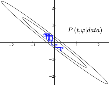
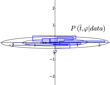
In the statistics literature, (t,φ)𝑡𝜑(t,\varphi) has been referred to as an ancillary parameterization whereas (t~,φ)~𝑡𝜑(\widetilde{t},\varphi) is referred to as a sufficient parameterization. We note that the terms ancillary and sufficient parameterization have been used interchangeably with the nomenclature non-centered and centered parameterizations, respectively, in the statistics literature Roberts et al. (2003); Gelfand et al. (1995); Papaspiliopoulos and Roberts (2008); Papaspiliopoulos et al. (2007); Yu and Meng (2011). Figure 1 illustrates the difference between an ancillary versus sufficient posterior distribution for our simple two parameter model. The left plot shows the posterior density contours for the ancillary parameterization (t,φ)𝑡𝜑(t,\varphi), along with 20 steps of a Gibbs sampler. Conversely, the right plot shows the posterior density contours for the sufficient chain (t~,φ)~𝑡𝜑(\widetilde{t},\varphi) with 20 Gibbs steps. Notice that negative correlation in the ancillary parameterization manifests in near independence for the sufficient chain. Indeed, the slower the ancillary chain the faster the sufficient chain and vice-versa.
Refer to caption
Refer to caption
Figure 1.— Left: density contours of the ancillary chain P(t,φ|data)𝑃𝑡conditional𝜑dataP(t,\varphi|\text{data}) with 20 steps of a Gibbs sampler. Right: density contours of the sufficient chain P(t~,φ|data)𝑃~𝑡conditional𝜑dataP(\widetilde{t},\varphi|\text{data}) with 20 steps of a Gibbs sampler. This illustrates the general heuristic that a slowly converging ancillary chain translates to a quickly converging the sufficient chain.

IV. Ancillary versus sufficient parameters for the lensed CMB

The ancillary parameterization presented in the previous section is analogous to the lensed CMB problem as follows

data(x)data𝑥\displaystyle\text{data}(x) =T(x+ϕ(x))+n(x)analogous todata=t+φ+nformulae-sequenceabsent𝑇𝑥italic-ϕ𝑥𝑛𝑥analogous todata𝑡𝜑𝑛\displaystyle=T(x+\nabla\phi(x))+n(x)\quad\text{\bf\em analogous to}\quad\text{data}=t+\varphi+n

where the unlensed CMB temperature field T𝑇T and the lensing potential ϕitalic-ϕ\phi are the two unknown parameters. As was discussed in Section II the Gibbs chain based on the ancillary parameters T(x)𝑇𝑥T(x) and ϕ(x)italic-ϕ𝑥\phi(x) is exceedingly slow. This clearly motivates the following re-parameterization to sufficient parameters for the lensed CMB problem

data(x)data𝑥\displaystyle\text{data}(x) =T~(x)+n(x)analogous todata=t~+nformulae-sequenceabsent~𝑇𝑥𝑛𝑥analogous todata~𝑡𝑛\displaystyle=\widetilde{T}(x)+n(x)\quad\text{\bf\em analogous to}\quad\text{data}=\widetilde{t}+n

where now T~~𝑇\widetilde{T} denotes the lensed CMB temperature field with no noise or beam. The sufficient chain then proceeds as

T~i+1superscript~𝑇𝑖1\displaystyle\widetilde{T}^{i+1} P(T~|ϕi,data)similar-toabsent𝑃conditional~𝑇superscriptitalic-ϕ𝑖data\displaystyle\sim P(\widetilde{T}|\phi^{i},\text{data}) (3)
ϕi+1superscriptitalic-ϕ𝑖1\displaystyle\phi^{i+1} P(ϕ|T~i+1,data).similar-toabsent𝑃conditionalitalic-ϕsuperscript~𝑇𝑖1data\displaystyle\sim P(\phi|\widetilde{T}^{i+1},\text{data}). (4)

In Section VI we adapt an iterative message passing algorithm, originally developed in Elsner and Wandelt (2013); Jasche and Lavaux (2015), for Wiener filtering and sampling from (3). In Section V we derive a Hamiltonian Markov Chain algorithm to sample from (4). Our Hamiltonian Markov Chain algorithm relies on an approximation—motivated again by the two parameter system—we call anti-lensing.

IV.1. Anti-lensing approximation

In the two parameter analogy from Section III, the relation between the sufficient parameter t~~𝑡\widetilde{t} and the ancillary parameter t𝑡t is given by t~φ=t~𝑡𝜑𝑡\widetilde{t}-\varphi=t. The corresponding relation for CMB lensing we refer to as anti-lensing:

T~(xϕ(x)anti-lensing)T(x).~𝑇subscript𝑥italic-ϕ𝑥anti-lensing𝑇𝑥\widetilde{T}(\,\underbrace{x-\nabla\phi(x)}_{\text{\small anti-lensing}}\,)\approx T(x). (5)

We distinguish between inverse lensing and anti-lensing. Inverse lensing denotes the true coordinate displacement which, when applied to T~~𝑇\widetilde{T}, recovers the unlensed T𝑇T. Conversely, anti-lensing is given by ϕitalic-ϕ-\nabla\phi and approximates inverse lensing.

To examine the difference between anti-lensing and inverse lensing notice that an extra divergence-free potential is needed to model the inverse lensing displacement field. Indeed, let f(x):=x+ϕ(x)assign𝑓𝑥𝑥italic-ϕ𝑥f(x):=x+\nabla\phi(x) denote the lensing map. With this notation we have

T~(x)=T(f(x)) and T(x)=T~(f1(x))formulae-sequence~𝑇𝑥𝑇𝑓𝑥 and 𝑇𝑥~𝑇superscript𝑓1𝑥\widetilde{T}(x)=T(f(x))\quad\text{ and }\quad T(x)=\widetilde{T}(f^{-1}(x))

where f1superscript𝑓1f^{-1} is the inverse lensing map that satisfies x=f1(f(x))𝑥superscript𝑓1𝑓𝑥x=f^{-1}(f(x)). Now let d(x)𝑑𝑥d(x) denote the displacement vector field for inverse lensing so that f1(x)=x+d(x)superscript𝑓1𝑥𝑥𝑑𝑥f^{-1}(x)=x+d(x). Therefore x=f1(f(x))=f(x)+d(f(x))𝑥superscript𝑓1𝑓𝑥𝑓𝑥𝑑𝑓𝑥x=f^{-1}(f(x))=f(x)+d(f(x)). In particular d(f(x))=xf(x)=ϕ(x)𝑑𝑓𝑥𝑥𝑓𝑥italic-ϕ𝑥d(f(x))=x-f(x)=-\nabla\phi(x) which gives

d(x)=ϕ(f1(x)).𝑑𝑥italic-ϕsuperscript𝑓1𝑥d(x)=-\nabla\phi(f^{-1}(x)).

This implies that the inverse lensing displacement is modeled as a warped version of the curl-free vector field ϕitalic-ϕ-\nabla\phi (warped by f1superscript𝑓1f^{-1}). This warping introduces a non-zero divergence-free term (just as lensing adds non-zero B-mode power in the CMB polarization).

To illustrate the expected magnitudes of the divergence-free and curl-free terms, start with a Helmholtz decomposition of the inverse lensing displacement: d(x)=ϕinv(x)ψinv(x),𝑑𝑥superscriptitalic-ϕinv𝑥superscriptperpendicular-tosuperscript𝜓inv𝑥d(x)=-\nabla\phi^{\text{inv}}(x)-\nabla^{\perp}\psi^{\text{inv}}(x), where (y,x)\nabla^{\perp}\equiv\bigr{(}-\frac{\partial}{\partial y},\frac{\partial}{\partial x}\bigl{)} and ψinvsuperscript𝜓inv\psi^{\text{inv}} denotes a stream function potential which models a field rotation so that

T~(xϕinv(x)ψinv(x)inverse lensing)~𝑇subscript𝑥superscriptitalic-ϕinv𝑥superscriptperpendicular-tosuperscript𝜓inv𝑥inverse lensing\displaystyle\widetilde{T}\bigl{(}\,\underbrace{x-\nabla\phi^{\text{inv}}(x)-\nabla^{\perp}\psi^{\text{inv}}(x)}_{\text{\small inverse lensing}}\,\bigr{)} =T(x).absent𝑇𝑥\displaystyle=T(x).

Due to the fact that the expected size of the inverse lensing displacement d(x)𝑑𝑥d(x) is on the order of arcmin but the correlation length scale of ϕitalic-ϕ\phi is on the order of degrees we claim that ϕ(f1(x))italic-ϕsuperscript𝑓1𝑥-\nabla\phi(f^{-1}(x)) is well approximated by ϕ(x)italic-ϕ𝑥-\nabla\phi(x). In particular, the divergence-free term ψinvsuperscriptperpendicular-tosuperscript𝜓inv-\nabla^{\perp}\psi^{\text{inv}} is small and

ϕitalic-ϕ\displaystyle-\nabla\phi ϕinvϕinvψinv=d.absentsuperscriptitalic-ϕinvsuperscriptitalic-ϕinvsuperscriptperpendicular-tosuperscript𝜓inv𝑑\displaystyle\approx-\nabla\phi^{\text{inv}}\approx-\nabla\phi^{\text{inv}}-\nabla^{\perp}\psi^{\text{inv}}=d. (6)

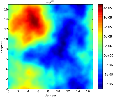
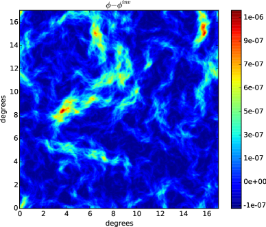
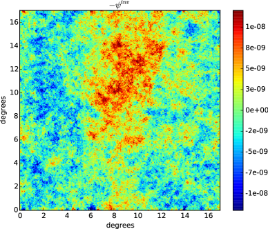
Figure 2 illustrates the magnitudes of the above terms. The anti-lensing potential ϕitalic-ϕ-\phi is shown (upper-left) along with the corresponding inverse lensing potential ϕinvsuperscriptitalic-ϕinv-\phi^{\text{inv}} (upper-right). The difference ϕϕinvitalic-ϕsuperscriptitalic-ϕinv\phi-\phi^{\text{inv}} is also shown (bottom left) along with the stream function ψinvsuperscript𝜓inv-\psi^{\text{inv}} (bottom-right). Clearly, the magnitude of the difference ϕinvϕsuperscriptitalic-ϕinvitalic-ϕ\phi^{\text{inv}}-\phi and ψinvsuperscript𝜓inv-\psi^{\text{inv}} is sub-dominant to estimation error expected in current lensing experimental conditions.

Refer to caption
Refer to caption
Refer to caption
Refer to caption
Figure 2.— The difference between anti-lensing and inverse lensing. Upper left: anti-lensing potential ϕitalic-ϕ-\phi. Upper right: The inverse lensing potential ϕinvsuperscriptitalic-ϕinv-\phi^{\text{inv}}. Bottom left: The difference ϕinvϕsuperscriptitalic-ϕinvitalic-ϕ\phi^{\text{inv}}-\phi. Bottom right: The inverse lensing stream function ψinvsuperscript𝜓inv-\psi^{\text{inv}}.

V. Hamiltonian Monte Carlo sampler for P(ϕ|T~,data)𝑃conditionalitalic-ϕ~𝑇dataP(\phi|\widetilde{T},\text{\rm data})

The Hamiltonian Monte Carlo (HMC) algorithm is an iterative sampling algorithm designed to mitigate the low-acceptance rate of the Metropolis-Hastings algorithm when working in high dimension. A nice review of HMC can be found in Neal (2011). For applications of HMC in cosmology see Hajian (2007); Taylor et al. (2008); Elsner and Wandelt (2010); Jasche et al. (2010); Jasche and Wandelt (2012); Jasche and Wandelt (2013a, b). In the present case we utilize the HMC algorithm to produce samples of ϕitalic-ϕ\phi from P(ϕ|T~,data)𝑃conditionalitalic-ϕ~𝑇dataP(\phi|\widetilde{T},\text{\rm data}). The key to making HMC work for lensing is to parameterize ϕitalic-ϕ\phi in terms of it’s Fourier transform. One can then utilize Claim 1, presented below, to efficiently compute the gradient of the log conditional density of P(ϕ|T~,data)𝑃conditionalitalic-ϕ~𝑇dataP(\phi|\widetilde{T},\text{\rm data}), which is a necessary computation for the HMC algorithm.

Notation: Throughout the remainder of this paper, the Fourier transform of any function f(x)𝑓𝑥f(x) will be denoted by flsubscript𝑓𝑙f_{l} or fksubscript𝑓𝑘f_{k} so that fl=2eixlf(x)dx2πsubscript𝑓𝑙subscriptsuperscript2superscript𝑒𝑖𝑥𝑙𝑓𝑥𝑑𝑥2𝜋f_{l}=\int_{\mathbb{R}^{2}}e^{-ix\cdot l}f(x)\frac{dx}{2\pi} and f(x)=2eixlfldl2π𝑓𝑥subscriptsuperscript2superscript𝑒𝑖𝑥𝑙subscript𝑓𝑙𝑑𝑙2𝜋f(x)=\int_{\mathbb{R}^{2}}e^{ix\cdot l}f_{l}\frac{dl}{2\pi} where l2𝑙superscript2l\in\mathbb{R}^{2} is a two dimensional frequency vector and x2𝑥superscript2x\in\mathbb{R}^{2} is a two dimensional spatial coordinate.

To describe the HMC algorithm let ϕbold-italic-ϕ\boldsymbol{\phi} denote the concatenation of the real and imaginary parts of ϕlsubscriptitalic-ϕ𝑙\phi_{l} as l𝑙l ranges through discrete frequencies l𝑙l ranging up to a pre-specified |l|maxsubscript𝑙𝑚𝑎𝑥|l|_{max} (but excluding half of the Fourier frequencies due to the Hermitian symmetry associated with the Fourier transform of a real field). Note that ϕbold-italic-ϕ\boldsymbol{\phi} is a vector of real numbers. Let P(ϕ|T~,data)𝑃conditionalbold-italic-ϕ~𝑇dataP(\boldsymbol{\phi}|\widetilde{T},\text{data}) denote the density of ϕbold-italic-ϕ\boldsymbol{\phi} given T~~𝑇\widetilde{T} and the data. Let 𝒑𝒑\boldsymbol{p} denote a ‘momentum’ vector and 𝒎𝒎\boldsymbol{m} denote a ‘mass’ vector, which are both the same length as ϕbold-italic-ϕ\boldsymbol{\phi}. The Hamiltonian is a function of ϕbold-italic-ϕ\boldsymbol{\phi} and 𝒑𝒑\boldsymbol{p} and is defined as follows

H(ϕ,𝒑):=logP(ϕ|T~,data)+k𝒑k22𝒎k2.assign𝐻bold-italic-ϕ𝒑𝑃conditionalbold-italic-ϕ~𝑇datasubscript𝑘superscriptsubscript𝒑𝑘22superscriptsubscript𝒎𝑘2H(\boldsymbol{\phi},\boldsymbol{p}):=-\log P(\boldsymbol{\phi}|\widetilde{T},\text{data})+\sum_{k}\frac{\boldsymbol{p}_{k}^{2}}{2\boldsymbol{m}_{k}^{2}}.

This Hamiltonian generates a time-dependent evolution of ϕbold-italic-ϕ\boldsymbol{\phi} and 𝒑𝒑\boldsymbol{p} given by

dϕtdt𝑑superscriptbold-italic-ϕ𝑡𝑑𝑡\displaystyle\frac{d\boldsymbol{\phi}^{t}}{dt} =𝒑H(ϕt,𝒑t)absentsubscript𝒑𝐻superscriptbold-italic-ϕ𝑡superscript𝒑𝑡\displaystyle=\phantom{-}\nabla_{\boldsymbol{p}}H(\boldsymbol{\phi}^{t},\boldsymbol{p}^{t})
d𝒑tdt𝑑superscript𝒑𝑡𝑑𝑡\displaystyle\frac{d\boldsymbol{p}^{t}}{dt} =ϕH(ϕt,𝒑t).absentsubscriptbold-italic-ϕ𝐻superscriptbold-italic-ϕ𝑡superscript𝒑𝑡\displaystyle=-\nabla_{\boldsymbol{\phi}}H(\boldsymbol{\phi}^{t},\boldsymbol{p}^{t}).

The HMC is a discrete version of this time-dynamic equation, using a leapfrog method, which produces a Markov chain (ϕ1,𝒑1),(ϕ2,𝒑2),subscriptbold-italic-ϕ1subscript𝒑1subscriptbold-italic-ϕ2subscript𝒑2(\boldsymbol{\phi}_{1},\boldsymbol{p}_{1}),(\boldsymbol{\phi}_{2},\boldsymbol{p}_{2}),\ldots where the ithsuperscript𝑖thi^{\text{th}} iteration is given by Algorithm 1 below.

Algorithm 1 ithsuperscript𝑖thi^{\text{th}} step of the Hamiltonian Markov Chain
1:Set ϕ0:=ϕi1assignsuperscriptbold-italic-ϕ0subscriptbold-italic-ϕ𝑖1\boldsymbol{\phi}^{0}:=\boldsymbol{\phi}_{i-1} and simulate 𝒑0𝒩(0,Λm)similar-tosuperscript𝒑0𝒩0subscriptΛ𝑚\boldsymbol{p}^{0}\sim\mathcal{N}(0,\Lambda_{m}) where ΛmsubscriptΛ𝑚\Lambda_{m} is diagonal with diag(Λm)=𝒎𝑑𝑖𝑎𝑔subscriptΛ𝑚𝒎diag(\Lambda_{m})=\boldsymbol{m}.
2:Recursively compute ϕkϵsuperscriptbold-italic-ϕ𝑘italic-ϵ\boldsymbol{\phi}^{k\epsilon} and 𝒑kϵsuperscript𝒑𝑘italic-ϵ\boldsymbol{p}^{k\epsilon} for k=1,,n𝑘1𝑛k=1,\ldots,n using the following equations:
ϕt+ϵsuperscriptbold-italic-ϕ𝑡italic-ϵ\displaystyle\boldsymbol{\phi}^{t+\epsilon} :=ϕt+ϵΛm1[𝒑tϵ2ϕH(ϕt,𝒑t)],assignabsentsuperscriptbold-italic-ϕ𝑡italic-ϵsuperscriptsubscriptΛ𝑚1delimited-[]superscript𝒑𝑡italic-ϵ2subscriptbold-italic-ϕ𝐻superscriptbold-italic-ϕ𝑡superscript𝒑𝑡\displaystyle:=\boldsymbol{\phi}^{t}+\epsilon\Lambda_{m}^{-1}\left[\boldsymbol{p}^{t}-\frac{\epsilon}{2}\nabla_{\boldsymbol{\phi}}H(\boldsymbol{\phi}^{t},\boldsymbol{p}^{t})\right],
𝒑t+ϵsuperscript𝒑𝑡italic-ϵ\displaystyle\boldsymbol{p}^{t+\epsilon} :=𝒑tϵ2[ϕH(ϕt,𝒑t)+ϕH(ϕt+ϵ,𝒑t)].assignabsentsuperscript𝒑𝑡italic-ϵ2delimited-[]subscriptbold-italic-ϕ𝐻superscriptbold-italic-ϕ𝑡superscript𝒑𝑡subscriptbold-italic-ϕ𝐻superscriptbold-italic-ϕ𝑡italic-ϵsuperscript𝒑𝑡\displaystyle:=\boldsymbol{p}^{t}-\frac{\epsilon}{2}\Bigl{[}\nabla_{\boldsymbol{\phi}}H(\boldsymbol{\phi}^{t},\boldsymbol{p}^{t})+\nabla_{\boldsymbol{\phi}}H(\boldsymbol{\phi}^{t+\epsilon},\boldsymbol{p}^{t})\Bigr{]}.
3:Simulate u𝒰(0,1)similar-to𝑢𝒰01u\sim\mathcal{U}(0,1), and define p:=min(1,eH(ϕnϵ,𝒑nϵ)/eH(ϕ0,𝒑0))assign𝑝1superscript𝑒𝐻superscriptbold-italic-ϕ𝑛italic-ϵsuperscript𝒑𝑛italic-ϵsuperscript𝑒𝐻superscriptbold-italic-ϕ0superscript𝒑0p:=\min\left(1,{e^{-H(\boldsymbol{\phi}^{n\epsilon},\boldsymbol{p}^{n\epsilon})}}/{e^{-H(\boldsymbol{\phi}^{0},\boldsymbol{p}^{0})}}\right).
4:If u<p𝑢𝑝u<p, set ϕi:=ϕnϵassignsubscriptbold-italic-ϕ𝑖superscriptbold-italic-ϕ𝑛italic-ϵ\boldsymbol{\phi}_{i}:=\boldsymbol{\phi}^{n\epsilon}, otherwise set ϕi:=ϕi1assignsubscriptbold-italic-ϕ𝑖subscriptbold-italic-ϕ𝑖1\boldsymbol{\phi}_{i}:=\boldsymbol{\phi}_{i-1}.

The HMC algorithm is notoriously sensitive to tuning parameters. The prevailing wisdom (see Neal (2011) page 22, for example) is that one should set 𝒎𝒎\boldsymbol{m} to match the reciprocal of the posterior variance of ϕbold-italic-ϕ\boldsymbol{\phi}. For the simulation presented in Section VII we simply set 𝒎l1subscriptsuperscript𝒎1𝑙\boldsymbol{m}^{-1}_{l} to be nearly proportional to Clϕϕsuperscriptsubscript𝐶𝑙italic-ϕitalic-ϕC_{l}^{\phi\phi} with a slight attenuation at low wavenumber. In particular, we set 𝒎l1:=2×10²[34+14tanh(|l|1500200)]Clϕϕδ0assignsuperscriptsubscript𝒎𝑙12superscript102delimited-[]3414𝑙1500200superscriptsubscript𝐶𝑙italic-ϕitalic-ϕsubscript𝛿0\boldsymbol{m}_{l}^{-1}:=2\times 10^{2}\bigl{[}\frac{3}{4}+\frac{1}{4}\tanh(\frac{|l|-1500}{200})\bigr{]}C_{l}^{\phi\phi}\delta_{0} where δlsubscript𝛿𝑙\delta_{l} is a discrete dirac in Fourier space. This choice was motivated by the fact that the high frequency terms ϕlsubscriptitalic-ϕ𝑙\phi_{l} are not well constrained by the posterior distribution which results in a posterior variance closely matching Clϕϕsuperscriptsubscript𝐶𝑙italic-ϕitalic-ϕC_{l}^{\phi\phi}. The remaining parameters of Algorithm 1 are set to n=30𝑛30n=30 and ϵ=2×10³uitalic-ϵ2superscript103𝑢\epsilon=2\times 10^{-3}u where u𝑢u is a uniform (0,1)01(0,1) random variable sampled anew at each pass of Algorithm 1 (the use of random ϵitalic-ϵ\epsilon is designed to avoid resonant frequencies, as advocated in Taylor et al. (2008)).

The key difficulty in using Algorithm 1 is the computation of the ϕH(ϕt,𝒑t)subscriptbold-italic-ϕ𝐻superscriptbold-italic-ϕ𝑡superscript𝒑𝑡\nabla_{\boldsymbol{\phi}}H(\boldsymbol{\phi}^{t},\boldsymbol{p}^{t}), or equivalently the computation of ϕlogP(ϕ|T~,data)subscriptbold-italic-ϕ𝑃conditionalbold-italic-ϕ~𝑇data\nabla_{\boldsymbol{\phi}}\log P(\boldsymbol{\phi}|\widetilde{T},\text{data}). The number of frequencies is extremely large and therefore, any slow computation of the gradients will present a serious bottleneck. The follow claim shows that the gradient of the log density of P(ϕ|T~,data)𝑃conditionalitalic-ϕ~𝑇dataP(\phi|\widetilde{T},\text{data}), with respect to the Fourier basis of ϕitalic-ϕ\phi, can be computed quickly with Fourier and inverse Fourier transforms.

Claim 1.

Under the anti-lensing approximation (5) for any nonzero frequency vector l(l1,l2)2𝑙subscript𝑙1subscript𝑙2superscript2l\equiv(l_{1},l_{2})\in\mathbb{R}^{2}

ϕllogP(ϕ|T~,data)ϕlClϕϕq=1,2ilq2eixlAq(x)B(x)dx2πproportional-tosubscriptitalic-ϕ𝑙𝑃conditionalitalic-ϕ~𝑇datasubscriptitalic-ϕ𝑙subscriptsuperscript𝐶italic-ϕitalic-ϕ𝑙subscript𝑞12𝑖subscript𝑙𝑞subscriptsuperscript2superscript𝑒𝑖𝑥𝑙superscript𝐴𝑞𝑥𝐵𝑥𝑑𝑥2𝜋\frac{\partial}{\partial\phi_{l}}\log P(\phi|\widetilde{T},\text{\rm data})\propto-\frac{\phi_{l}}{C^{\phi\phi}_{l}}-\sum_{q=1,2}il_{q}\int_{\mathbb{R}^{2}}e^{-ix\cdot l}A^{q}(x)B(x)\frac{dx}{2\pi} (7)

where ϕl= reϕl+i imϕlsubscriptitalic-ϕ𝑙 resubscriptitalic-ϕ𝑙𝑖 imsubscriptitalic-ϕ𝑙\phi_{l}=\text{\,\rm re}\phi_{l}+i\text{\,\rm im}\phi_{l}, ϕl reϕl+i imϕlsubscriptitalic-ϕ𝑙 resubscriptitalic-ϕ𝑙𝑖 imsubscriptitalic-ϕ𝑙\frac{\partial}{\partial\phi_{l}}\equiv\frac{\partial}{\partial\text{\,\rm re}\phi_{l}}+i\frac{\partial}{\partial\text{\,\rm im}\phi_{l}} and

Blsubscript𝐵𝑙\displaystyle B_{l} 1ClTTeixlT~(xϕ(x))dx2πabsent1superscriptsubscript𝐶𝑙𝑇𝑇superscript𝑒𝑖𝑥𝑙~𝑇𝑥italic-ϕ𝑥𝑑𝑥2𝜋\displaystyle\equiv\frac{1}{C_{l}^{TT}}\int e^{-ix\cdot l}\widetilde{T}(x-\nabla\phi(x))\frac{dx}{2\pi} (8)
Aq(x)superscript𝐴𝑞𝑥\displaystyle A^{q}(x) T~xq(xϕ(x)).absent~𝑇subscript𝑥𝑞𝑥italic-ϕ𝑥\displaystyle\equiv\frac{\partial\widetilde{T}}{\partial x_{q}}\bigl{(}x-\nabla\phi(x)\bigr{)}. (9)

An important fact used in the derivation of (7) is that the lensing and anti-lensing operator is invertible. For example, if ϕ(x)italic-ϕ𝑥\phi(x) and T~(x)~𝑇𝑥\widetilde{T}(x) are known at all pixel locations x𝑥x, then it is possible to perfectly reconstruct T(x)𝑇𝑥T(x). This implies that the anti-lensing operation (which is a linear action on the CMB) can be represented as an infinitesimal permutation matrix. Therefore, the determinant of the anti-lensing operator det(dT~ϕ/dT~)𝑑superscript~𝑇italic-ϕ𝑑~𝑇\det(d\widetilde{T}^{\phi}/d\widetilde{T}) equals 111, where T~ϕ(x)T~(xϕ(x))superscript~𝑇italic-ϕ𝑥~𝑇𝑥italic-ϕ𝑥\widetilde{T}^{\phi}(x)\equiv\widetilde{T}(x-\nabla\phi(x)). Now, to compute the likelihood surface P(ϕ|T~,data)𝑃conditionalitalic-ϕ~𝑇dataP(\phi|\widetilde{T},\text{\rm data}) as a function of ϕitalic-ϕ\phi we obtain the following formula:

P(ϕ|T~,data)𝑃conditionalitalic-ϕ~𝑇data\displaystyle P(\phi|\widetilde{T},\text{\rm data}) =P(ϕ|T~)absent𝑃conditionalitalic-ϕ~𝑇\displaystyle=P(\phi|\widetilde{T})
P(T~|ϕ)P(ϕ)proportional-toabsent𝑃conditional~𝑇italic-ϕ𝑃italic-ϕ\displaystyle\propto P(\widetilde{T}|\phi)P(\phi)
=|det(dT~ϕ/dT~)|=1P(T~ϕ|ϕ)P(ϕ)absentsubscript𝑑superscript~𝑇italic-ϕ𝑑~𝑇absent1𝑃conditionalsuperscript~𝑇italic-ϕitalic-ϕ𝑃italic-ϕ\displaystyle=\underbrace{|\det(d\widetilde{T}^{\phi}/d\widetilde{T})|}_{=1}P(\widetilde{T}^{\phi}|\phi)P(\phi)

where P(T~ϕ|ϕ)𝑃conditionalsuperscript~𝑇italic-ϕitalic-ϕP(\widetilde{T}^{\phi}|\phi) represents the likelihood that T~ϕsuperscript~𝑇italic-ϕ\widetilde{T}^{\phi} is statistically unlensed by ϕitalic-ϕ\phi. In other words, P(T~ϕ|ϕ)𝑃conditionalsuperscript~𝑇italic-ϕitalic-ϕP(\widetilde{T}^{\phi}|\phi) measures the likelihood that T~ϕsuperscript~𝑇italic-ϕ\widetilde{T}^{\phi} is an isotropic Gaussian random field with spectral density ClTTsuperscriptsubscript𝐶𝑙𝑇𝑇C_{l}^{TT}. This explains the following characterization of the log likelihood of ϕitalic-ϕ\phi given T~~𝑇\widetilde{T} and the data:

logP(ϕ|T~,data)=c122[|T~kϕ|2CkTT+|ϕk|2Ckϕϕ]𝑑k𝑃conditionalitalic-ϕ~𝑇data𝑐12subscriptsuperscript2delimited-[]superscriptsuperscriptsubscript~𝑇𝑘italic-ϕ2superscriptsubscript𝐶𝑘𝑇𝑇superscriptsubscriptitalic-ϕ𝑘2superscriptsubscript𝐶𝑘italic-ϕitalic-ϕdifferential-d𝑘\displaystyle\log P(\phi|\widetilde{T},\text{\rm data})=c-\frac{1}{2}\int_{\mathbb{R}^{2}}\left[\frac{\bigl{|}\widetilde{T}_{k}^{\phi}\bigr{|}^{2}}{C_{k}^{TT}}+\frac{|\phi_{k}|^{2}}{C_{k}^{\phi\phi}}\right]dk (10)

where c𝑐c is a constant which does not depend on ϕitalic-ϕ\phi. The remaining details of the derivation of Claim 1 is left to the appendix.

It is instructive to compare the gradient calculation (7) with the quadratic estimate of ϕitalic-ϕ\phi developed in Hu (2001); Hu and Okamoto (2002). The quadratic estimate, applied to observations of the form T~(x)+n(x)~𝑇𝑥𝑛𝑥\widetilde{T}(x)+n(x), is given by

ϕ^l=Nlq=1,2ilq2eixlAq(x)B(x)dx2πsubscript^italic-ϕ𝑙subscript𝑁𝑙subscript𝑞12𝑖subscript𝑙𝑞subscriptsuperscript2superscript𝑒𝑖𝑥𝑙superscript𝐴𝑞𝑥𝐵𝑥𝑑𝑥2𝜋\hat{\phi}_{l}=-N_{l}\sum_{q=1,2}il_{q}\int_{\mathbb{R}^{2}}e^{-ix\cdot l}A^{q}(x)B(x)\frac{dx}{2\pi} (11)

where Bl[ClT~T~+Clnn]1[T~l+nl]subscript𝐵𝑙superscriptdelimited-[]superscriptsubscript𝐶𝑙~𝑇~𝑇superscriptsubscript𝐶𝑙𝑛𝑛1delimited-[]subscript~𝑇𝑙subscript𝑛𝑙B_{l}\equiv\bigl{[}C_{l}^{\widetilde{T}\widetilde{T}}+C_{l}^{nn}\bigr{]}^{-1}\bigl{[}\widetilde{T}_{l}+n_{l}\bigr{]}, Alqilq[ClTT][ClT~T~+Clnn]1[T~l+nl]subscriptsuperscript𝐴𝑞𝑙𝑖subscript𝑙𝑞delimited-[]superscriptsubscript𝐶𝑙𝑇𝑇superscriptdelimited-[]superscriptsubscript𝐶𝑙~𝑇~𝑇superscriptsubscript𝐶𝑙𝑛𝑛1delimited-[]subscript~𝑇𝑙subscript𝑛𝑙A^{q}_{l}\equiv il_{q}\bigl{[}C_{l}^{TT}\bigr{]}\bigl{[}C_{l}^{\widetilde{T}\widetilde{T}}+C_{l}^{nn}\bigr{]}^{-1}\bigl{[}\widetilde{T}_{l}+n_{l}\bigr{]} and

Nl1122(l(k+l)Ck+lTTlkCkTT)2(Ck+lT~T~+Ck+lnn)(CkT~T~+Cknn)dk(2π)2.superscriptsubscript𝑁𝑙112subscriptsuperscript2superscript𝑙𝑘𝑙subscriptsuperscript𝐶𝑇𝑇𝑘𝑙𝑙𝑘subscriptsuperscript𝐶𝑇𝑇𝑘2subscriptsuperscript𝐶~𝑇~𝑇𝑘𝑙superscriptsubscript𝐶𝑘𝑙𝑛𝑛subscriptsuperscript𝐶~𝑇~𝑇𝑘superscriptsubscript𝐶𝑘𝑛𝑛𝑑𝑘superscript2𝜋2N_{l}^{-1}\equiv\frac{1}{2}\int_{\mathbb{R}^{2}}\frac{\bigl{(}l\cdot(k+l)C^{TT}_{k+l}-l\cdot kC^{TT}_{k}\bigr{)}^{2}}{\bigl{(}C^{\widetilde{T}\widetilde{T}}_{k+l}+C_{k+l}^{nn}\bigr{)}\bigl{(}C^{\widetilde{T}\widetilde{T}}_{k}+C_{k}^{nn}\bigr{)}}\frac{dk}{(2\pi)^{2}}.

The term Nlsubscript𝑁𝑙N_{l} is radially symmetric in frequency l𝑙l and corresponds to a normalization which makes the quadratic estimate unbiased up to first order. After substituting ClT~T~+ClnnClTTsuperscriptsubscript𝐶𝑙~𝑇~𝑇superscriptsubscript𝐶𝑙𝑛𝑛superscriptsubscript𝐶𝑙𝑇𝑇C_{l}^{\widetilde{T}\widetilde{T}}+C_{l}^{nn}\rightarrow C_{l}^{TT} and nl0subscript𝑛𝑙0n_{l}\rightarrow 0 in the formula for the quadratic estimate, one obtains

ϕllogP(ϕ|T~,data)|ϕ=0=ϕ^lNl.evaluated-atsubscriptitalic-ϕ𝑙𝑃conditionalitalic-ϕ~𝑇dataitalic-ϕ0subscript^italic-ϕ𝑙subscript𝑁𝑙\frac{\partial}{\partial\phi_{l}}\log P(\phi|\widetilde{T},\text{\rm data})\bigr{|}_{\phi=0}=\frac{\hat{\phi}_{l}}{N_{l}}.

Indeed, an approximate Newton step, using (7), is an accurate approximation to the quadratic estimate ϕ^lsubscript^italic-ϕ𝑙\hat{\phi}_{l}. This illustrates how the parameterization (T~,ϕ)~𝑇italic-ϕ(\widetilde{T},\phi) results in Gibbs iterations which make drastic moves, on the order of the size of the quadratic estimate.

One of the features of the quadratic estimate is that the fast Fourier transform (FFT) and inverse fast Fourier transform (IFFT) can be used to compute ϕ^lsubscript^italic-ϕ𝑙\hat{\phi}_{l} for all frequencies l𝑙l. Naively computing the quadratic form of the quadratic estimate requires O(n2)𝑂superscript𝑛2O(n^{2}) flops, rather than the O(nlogn)𝑂𝑛𝑛O(n\log n) flops obtained by the FFT/IFFT method, where n𝑛n denotes the number of pixels. We note that Claim 1 establishes that the gradient computation inherits a similar FFT/IFFT characterization to compute ϕllogP(ϕ|T~,data)subscriptitalic-ϕ𝑙𝑃conditionalitalic-ϕ~𝑇data\frac{\partial}{\partial\phi_{l}}\log P(\phi|\widetilde{T},\text{\rm data}) at all frequencies l𝑙l, in O(nlogn)𝑂𝑛𝑛O(n\log n) flops. Since this gradient computation needs to be embedded in a Hamiltonian Markov step within a Gibbs Chain, the computation efficiency gained by the FFT/IFFT is absolutely crucial.

VI. Iterative message passing algorithm for P(T~|ϕ,data)𝑃conditional~𝑇italic-ϕdataP(\widetilde{T}|\phi,\text{\rm data})

There are two natural ways to model the lensed CMB T~~𝑇\widetilde{T}. If one marginalizes out ϕitalic-ϕ\phi, then T~~𝑇\widetilde{T} is modeled as a non-Gaussian but isotropic random field. Conversely, if one conditions on ϕitalic-ϕ\phi the field T~~𝑇\widetilde{T} is modeled as a non-isotropic but Gaussian random field. The latter case is relevant for sampling from P(T~|ϕ,data)𝑃conditional~𝑇italic-ϕdataP(\widetilde{T}|\phi,\text{\rm data}) which is, therefore, simply a Gaussian conditional simulation problem. Unfortunately, the non-isotropic (indeed, non-stationary) nature of the conditional distribution of T~~𝑇\widetilde{T} presents serious computational challenges. In what follows we utilize a new iterative algorithm developed in Elsner and Wandelt (2013) for Gaussian conditional expectation when the signal is diagonalized in harmonic space that the noise is diagonalized in pixel space. The method we present here is similar to the Gibbs sampling adaptation of Jasche and Lavaux (2015).

Start by transforming each pixel location x𝑥x by the lensing operation x+ϕ(x)𝑥italic-ϕ𝑥x+\nabla\phi(x), while simultaneously preserving the data associated with that pixel. This effectively de-lenses data(x)=T(x+ϕ(x))+n(x)data𝑥𝑇𝑥italic-ϕ𝑥𝑛𝑥\text{data}(x)=T(x+\nabla\phi(x))+n(x) but produces observations on an irregular grid. In particular, one may switch to the lensed coordinates y=x+ϕ(x)𝑦𝑥italic-ϕ𝑥y=x+\nabla\phi(x) so that

(x+ϕ(x), data(x))(pixel, data) tuplesubscript𝑥italic-ϕ𝑥 data𝑥(pixel, data) tuple\displaystyle\underbrace{(x+\nabla\phi(x),\,\text{ data}(x))}_{\text{(pixel, data) tuple}} =(y,T(y)+n~(y))absent𝑦𝑇𝑦~𝑛𝑦\displaystyle=(y,\,T(y)+\tilde{n}(y))

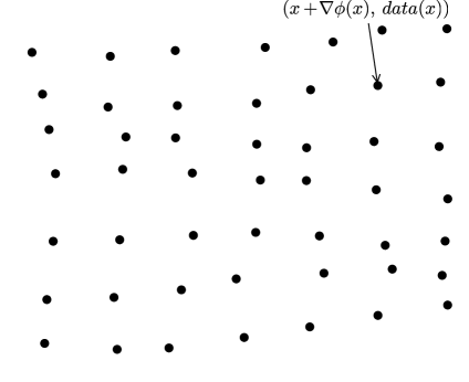
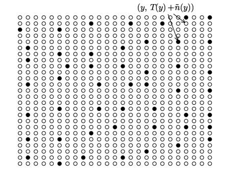
where n~(x+ϕ(x))=n(x)~𝑛𝑥italic-ϕ𝑥𝑛𝑥\tilde{n}(x+\nabla\phi(x))=n(x). Now the data (y,T(y)+n~(y))𝑦𝑇𝑦~𝑛𝑦(y,\,T(y)+\tilde{n}(y)) is arranged on an irregular grid in y𝑦y. This irregular grid is then embedded into a high resolution regular grid by nearest neighbor interpolation. The points y𝑦y which do not get assigned an observation T(y)+n~(y)𝑇𝑦~𝑛𝑦T(y)+\tilde{n}(y) under the interpolation we consider to be masked. Figure 3 illustrates this situation. The left hand plot shows the irregularly sampled data (x+ϕ(x), data(x))𝑥italic-ϕ𝑥 data𝑥(x+\nabla\phi(x),\,\text{ data}(x)) and the right hand plot shows the grid embedding. The filled dots represent observations of T(y)+n~(y)𝑇𝑦~𝑛𝑦T(y)+\tilde{n}(y) whereas the empty dots correspond to a masked observation of T(y)𝑇𝑦T(y). Finally we extend the definition of n~(y)~𝑛𝑦\tilde{n}(y) to have infinite variance over the masked region, whereby producing data T(y)+n~(y)𝑇𝑦~𝑛𝑦T(y)+\tilde{n}(y) over a dense regular grid in y𝑦y.

Refer to caption
Refer to caption
Figure 3.— This graphic illustrates how knowledge of ϕ(x)italic-ϕ𝑥\phi(x), used when sampling from the Gibbs step P(T~|ϕ,data)𝑃conditional~𝑇italic-ϕdataP(\widetilde{T}|\phi,\text{data}), converts white noise corrupted gridded observations of the lensed CMB into masked observations of the unlensed CMB on a more dense grid. The data associated with the original grid, indexed by x𝑥x, is moved via advection to the lensed grid x+ϕ(x)𝑥italic-ϕ𝑥x+\nabla\phi(x) seen at left. The right panel shows the lensed grid embedded into a higher resolution grid. The data, indexed by the dense regular grid on the right panel, is of the form T(y)+n~(y)𝑇𝑦~𝑛𝑦T(y)+\tilde{n}(y) where T(y)𝑇𝑦T(y) denotes the unlensed CMB and n~(y)~𝑛𝑦\tilde{n}(y) denotes the noise. The unobserved locations, represented by open circles, are characterized with an infinite variance for n~(y)~𝑛𝑦\tilde{n}(y).

As a intermediate step in producing a sample from P(T~|ϕ,data)𝑃conditional~𝑇italic-ϕdataP(\widetilde{T}|\phi,\text{\rm data}) we produce a conditional sample of T(y)𝑇𝑦T(y) given the observations T(y)+n~(y)𝑇𝑦~𝑛𝑦T(y)+\tilde{n}(y). The difficulty of this step is that n~(y)~𝑛𝑦\tilde{n}(y) is non-homogeneous noise—from the masking and any inhomogeneity in n(x)𝑛𝑥n(x)—and therefore it is not decorrelated by the Fourier transform. To handle this situation we adapted a new method for Gaussian conditional expectation developed in Elsner and Wandelt (2013). This method works particularly well for observations with large amounts of irregular masking, as in our case. The algorithm utilizes a messenger field which effectively behaves as a latent—signal plus white noise—model which is amenable to Gibbs sampling (Jasche and Lavaux, 2015).

The delensing algorithm described in this paper requires the capability to do fast constrained realization of non-lensed CMB. The embedding illustrated in Figure 3 means that each constrained realization needs to be computed on a mask with a great deal of structure on the scale of the pixels of dense grid. Several algorithms exist in the literature to solve the general problem of constrained Gaussian random field on a given mask and power spectrum: the conjugate gradient method (Wandelt et al., 2004; Eriksen et al., 2004), the multiscale conjugate gradient method (Smith et al., 2007), the multigrid method (Seljebotn et al., 2014), the Messenger algorithm (Elsner and Wandelt, 2013) and its variant the Gibbs-Messenger (Jasche and Lavaux, 2015).

Since the lensing potential changes from each iteration to the next, every constrained realization of non-lensed CMB needs to be computed for a different set of active points in the embedding grid. This effectively means that the solution is done for a different mask at every iteration. This rules out linear solvers that require expensive pre-computations, e.g. of pre-conditioners, that depend on the coefficient matrix of the system since that depends on the mask. We also require exact acceptance and higher speed than direct or standard iterative methods. This reduces the possibilities to either the Messenger algorithm or the Gibbs-Messenger.

The Gibbs-Messenger generates very fast constrained realizations that converge to the correct distribution in a statistical sense without iterating to a numerical solution (thus obviating the need to specify a colling schedule in Algorithm 2) for the price of losing independence between subsequent samples. In contrast the Messenger algorithm simulates independent constrained realisations, but requires iteration of the linear system. To ensure a numerically accurate solution implies a conservative choice of cooling schedule in Algorithm 2 (though this is still much faster than the alternatives described in the previous paragraph).

We adopt a hybrid approach where we occasionally generate an independent sample using the Messenger algorithm, and then generate many quick samples using the Gibbs-Messenger approach. The detailed choices for the cooling schedule and the number of samples between full Messenger solutions will be described in Section VII.

Algorithm 2 Algorithm for sampling from P(T|data)𝑃conditional𝑇dataP(T|\text{data}) where data(y)=T(y)+n~(y)data𝑦𝑇𝑦~𝑛𝑦\text{data}(y)=T(y)+\tilde{n}(y)
1:Set cooling schedule λ1λnsubscript𝜆1subscript𝜆𝑛\lambda_{1}\geq\ldots\geq\lambda_{n} where λn=1subscript𝜆𝑛1\lambda_{n}=1.
2:Decompose n~(y)~𝑛𝑦\tilde{n}(y) into a homogeneous part with variance σ¯2superscript¯𝜎2\bar{\sigma}^{2} and a non-homogeneous part with variance σ~2(y)superscript~𝜎2𝑦\tilde{\sigma}^{2}(y) so that

var(n~(y))=σ¯2+σ~2(y)var~𝑛𝑦superscript¯𝜎2superscript~𝜎2𝑦\text{var}(\tilde{n}(y))=\bar{\sigma}^{2}+\tilde{\sigma}^{2}(y)

where σ~2(y)=superscript~𝜎2𝑦\tilde{\sigma}^{2}(y)=\infty on all masked pixels y𝑦y. Notice that the spectral density of the homogeneous part is given by σ¯2dysuperscript¯𝜎2𝑑𝑦\bar{\sigma}^{2}dy where dy𝑑𝑦dy denotes the pixel grid area.
3:Initialize the fields M(y)𝑀𝑦M(y) and T(y)𝑇𝑦T(y) to be zero at all pixel locations y𝑦y.
4:Recursively update fields M(y)𝑀𝑦M(y) and T(y)𝑇𝑦T(y) by iterating the following steps for j=1,,n𝑗1𝑛j=1,\ldots,n:
  • \bullet

    Simulate a mean zero Gaussian random field Z(y)𝑍𝑦Z(y) which is independent across pixels and with pointwise variance (1λjσ¯2+1σ~2(y))1superscript1subscript𝜆𝑗superscript¯𝜎21superscript~𝜎2𝑦1\bigl{(}\frac{1}{\lambda_{j}\bar{\sigma}^{2}}+\frac{1}{\tilde{\sigma}^{2}(y)}\bigr{)}^{-1}.

  • \bullet

    Update M(y)data(y)λjσ¯2λjσ¯2+σ~2(y)+T(y)σ~2(y)λjσ¯2+σ~2(y)+Z(y)𝑀𝑦data𝑦subscript𝜆𝑗superscript¯𝜎2subscript𝜆𝑗superscript¯𝜎2superscript~𝜎2𝑦𝑇𝑦superscript~𝜎2𝑦subscript𝜆𝑗superscript¯𝜎2superscript~𝜎2𝑦𝑍𝑦M(y)\leftarrow\text{data}(y)\displaystyle\frac{\lambda_{j}\bar{\sigma}^{2}}{\lambda_{j}\bar{\sigma}^{2}+\tilde{\sigma}^{2}(y)}+T(y)\frac{\tilde{\sigma}^{2}(y)}{\lambda_{j}\bar{\sigma}^{2}+\tilde{\sigma}^{2}(y)}+Z(y).

  • \bullet

    Simulate a mean zero Gaussian random field, W(y)𝑊𝑦W(y), with spectral density WlWl=δll(1ClTT+1λjσ¯2dy)1delimited-⟨⟩subscript𝑊𝑙superscriptsubscript𝑊superscript𝑙subscript𝛿𝑙superscript𝑙superscript1subscriptsuperscript𝐶𝑇𝑇𝑙1subscript𝜆𝑗superscript¯𝜎2𝑑𝑦1\langle W_{l}W_{l^{\prime}}^{*}\rangle=\delta_{l-l^{\prime}}\bigl{(}\frac{1}{C^{TT}_{l}}+\frac{1}{\lambda_{j}\bar{\sigma}^{2}dy}\bigr{)}^{-1}

  • \bullet

    Update TlMlClTTClTT+λjσ¯2dy+Wlsubscript𝑇𝑙subscript𝑀𝑙subscriptsuperscript𝐶𝑇𝑇𝑙subscriptsuperscript𝐶𝑇𝑇𝑙subscript𝜆𝑗superscript¯𝜎2𝑑𝑦subscript𝑊𝑙T_{l}\leftarrow M_{l}\displaystyle\frac{C^{TT}_{l}}{C^{TT}_{l}+\lambda_{j}\bar{\sigma}^{2}dy}+W_{l}.

5:Return T(x)𝑇𝑥T(x).

The following algorithm describes the use of Algorithm 2 to produce a sample from P(T~|ϕ,data)𝑃conditional~𝑇italic-ϕdataP(\widetilde{T}|\phi,\text{\rm data}).

Algorithm 3 Sampling from P(T~|ϕ,data)𝑃conditional~𝑇italic-ϕdataP(\widetilde{T}|\phi,\text{\rm data})
1:Embedded the pixel/data pairs (x,data(x))𝑥data𝑥(x,\text{data}(x)) into observations of the form (y,T(y)+n~(y))𝑦𝑇𝑦~𝑛𝑦(y,T(y)+\tilde{n}(y)) where y𝑦y ranges over a high resolution regular grid as illustrated in the right plot of Figure 3.
2:Use Algorithm 2 to produce a sample TP(T|T+n~)similar-to𝑇𝑃conditional𝑇𝑇~𝑛T\sim P(T\,|\,T+\tilde{n}).
3:Return T~(x)=T(x+ϕ(x))~𝑇𝑥𝑇𝑥italic-ϕ𝑥\widetilde{T}(x)=T(x+\nabla\phi(x)).

At present, algorithms 2 and 3 are designed for the situation that the pixels are sufficiently small compared to the magnitude of ϕ(x)italic-ϕ𝑥\nabla\phi(x) and the noise is approximately white on these scales. Indeed, our goal is to explore the low noise and small beam experimental conditions where the quadratic estimate is known to be suboptimal (see Hirata and Seljak (2003a, b)). That being said, the only change needed to incorporate other experimental details in the Bayesian lensing methodology presented here, including foreground contaminants, is how one samples from P(T~|ϕ,data)𝑃conditional~𝑇italic-ϕdataP(\widetilde{T}|\phi,\text{\rm data}). Algorithms 2 and 3 take advantage of the special lensed-grid structure of the data when conditioning on ϕitalic-ϕ\phi to accomplish this goal. Adding different/new experimental details to the data will still result in a Gaussian constrained realization problem. We acknowledged that more complicated modeling of the data will most certainly introduce additional computational challenges. However, we consider these computational challenges to be sub-dominant to the fundamental bottleneck for Bayesian lensing which was the extremely slow mixing time of the original Gibbs formulation. Moreover, the structure of the new Gibbs formulation isolates all experimental details to the Gibbs step (4) where conditioning on the lensing potential ϕitalic-ϕ\phi results in a classic Gaussian constrained realization problem.

VII. Simulation example

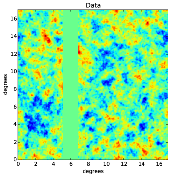
In this section we present a simulation to illustrate the methodology presented above. The simulated lensing potential used in this section, shown at left in Figure 5, is generated on a flat sky with periodic boundary conditions. The data, shown upper-left in Figure 6, is generated on 2 arcmin pixels with independent additive noise and masking. The noise level is set to 8.08.08.0 μK𝜇𝐾\mu K arcmin and the masking covers approximately 10% of the pixels. The parameters of the Bayesian lensing procedure are the Fourier modes of T~~𝑇\widetilde{T} and ϕitalic-ϕ\phi. For the lensing potential we set |l|maxsubscript𝑙max|l|_{\text{max}} to 460460~{}460. For this sky coverage the scale-resolution in Fourier space Δl=21Δ𝑙21\Delta l=21 yields 150015001500 unknown Fourier coefficients for ϕlsubscriptitalic-ϕ𝑙\phi_{l}. The |l|maxsubscript𝑙max|l|_{\text{max}} of 270027002700 for the unlensed temperature T𝑇T is set in Algorithm 2 and corresponds to half of the Nyquist limit at 222 arcmin pixels.

Refer to caption
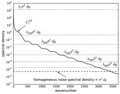
Figure 4.— This figure shows values of the cooling parameter λjsubscript𝜆𝑗\lambda_{j} for j=1,100,300,500,700,900𝑗1100300500700900j=1,100,300,500,700,900 used in Algorithm 2. This schedule is applied every 100thsuperscript100th100^{\text{th}} step in the Gibbs algorithm. In Algorithm 2, the value of λjσ¯2dysubscript𝜆𝑗superscript¯𝜎2𝑑𝑦\lambda_{j}\bar{\sigma}^{2}dy serves as the spectral density of artificial additive white noise in the latent field M(x)𝑀𝑥M(x). Therefore setting λjsubscript𝜆𝑗\lambda_{j} greater than 111, encourages fast mixing of Tlsubscript𝑇𝑙T_{l} at all frequency vectors l𝑙l such that ClTTλjσ¯2dyless-than-or-similar-tosuperscriptsubscript𝐶𝑙𝑇𝑇subscript𝜆𝑗superscript¯𝜎2𝑑𝑦C_{l}^{TT}\lesssim\lambda_{j}\bar{\sigma}^{2}dy. The cooling schedule shown above is an attempt to let λjsubscript𝜆𝑗\lambda_{j} approach 111 in such a way as to encourage all frequency vectors up to |l|maxsubscript𝑙max|l|_{\text{max}} to mix quickly.

We ran 101010 parallel Gibbs chains for a total of 250025002500 steps. The timings for each Gibbs iteration averaged approximately 200 seconds using a Dual Intel Xeon E5-2690 2.90GHz processor. Each chain was initially warmed up by replacing the HMC draws in the first 555 iterations with a gradient ascent. A burn-in of approximately 550550550 runs were discarded and the remaining runs were thinned by 100100100. The result is a total of 200200200 posterior samples. The cooling schedule for the iterative message passing algorithm was selected by numerical experimentation. Most of the Gibbs iterations set the cooling terms (λ1,,λ400)(1,,1)subscript𝜆1subscript𝜆40011(\lambda_{1},\ldots,\lambda_{400})\equiv(1,\ldots,1) in Algorithm 2. However, we did find it advantageous to periodically run a nontrivial 100010001000-step cooling schedule every 100thsuperscript100th100^{\text{th}} pass of the Gibbs algorithm. This nontrivial cooling schedule for λjsubscript𝜆𝑗\lambda_{j} is plotted in Figure 4 and is set in an attempt to encourage fast mixing of the Fourier modes Tlsubscript𝑇𝑙T_{l} up to |l|maxsubscript𝑙max|l|_{\text{max}}.

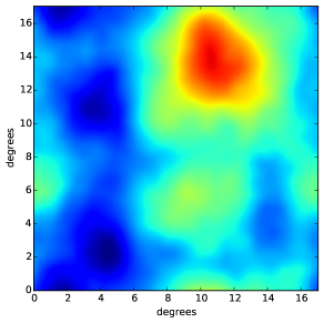
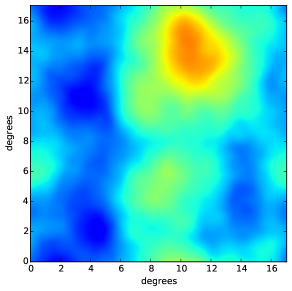
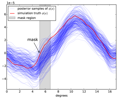
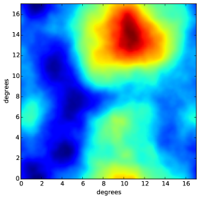
The best Bayesian estimate of ϕ(x)italic-ϕ𝑥\phi(x) corresponds to the posterior mean E(ϕ(x)|data)𝐸conditionalitalic-ϕ𝑥dataE(\phi(x)|\text{data}). This quantity is approximated by the average of the 200200200 draws from the Gibbs chain and is shown in the middle plot of Figure 5. The right plot of Figure 5 shows the quadratic estimate of ϕ(x)italic-ϕ𝑥\phi(x) for comparison. However, due to the difficulty when using the quadratic estimate in the presence of sky cuts, the quadratic estimate shown uses all of the data—including the pixels which are masked—in producing the estimate of ϕitalic-ϕ\phi. In general, one can see good agreement with E(ϕ(x)|data)𝐸conditionalitalic-ϕ𝑥dataE(\phi(x)|\text{data}) and ϕ(x)italic-ϕ𝑥\phi(x). Indeed, the effect of masking is visually undetectable as compared to the quadratic estimate. To get a better visualization of the individual draws from the posterior, the left plot in Figure 7 shows a horizontal cross section of the posterior draws of ϕ(x)italic-ϕ𝑥\phi(x) taken at vertical degree mark 12.7osuperscript12.7𝑜12.7^{o}.

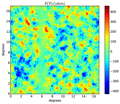
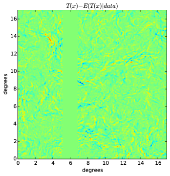
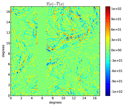
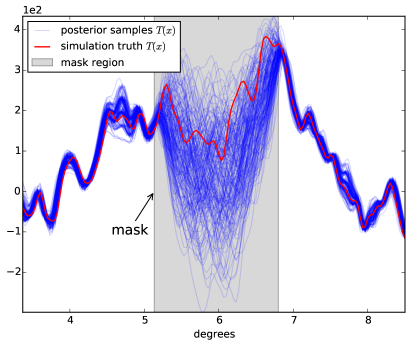
The Gibbs methodology presented here yields samples of the lensed CMB T~(x)~𝑇𝑥\widetilde{T}(x) and the lensing potential ϕ(x)italic-ϕ𝑥\phi(x) conditional on the data. Moreover, as a byproduct of Algorithm 3, we also obtain samples of the unlensed T(x)𝑇𝑥T(x) given the data. By averaging 200200200 draws from the Gibbs chain one can construct an approximation to E(T(x)|data)𝐸conditional𝑇𝑥dataE(T(x)|\text{data}), shown in the upper-right plot of Figure 6. In the bottom-left plot of Figure 6 we show the difference T(x)E(T(x)|data)𝑇𝑥𝐸conditional𝑇𝑥dataT(x)-E(T(x)|\text{data}). When compared to the nominal difference between lensed and unlensed CMB T(x)T~(x)𝑇𝑥~𝑇𝑥T(x)-\widetilde{T}(x), shown bottom-right in Figure 6, one can see that the Gibbs methodology is successful at delensing the observed CMB. To get a better visualization of the individual draws from the posterior, the right plot in Figure 7 shows a horizontal cross section of the posterior draws of T(x)𝑇𝑥T(x) taken at vertical degree mark 12.7osuperscript12.7𝑜12.7^{o} and is magnified near the masking region for better visual inspection.
Refer to caption
Refer to caption
Refer to caption
Figure 5.— Left: simulation truth ϕ(x)italic-ϕ𝑥\phi(x). Middle: posterior mean E(ϕ(x)|data)𝐸conditionalitalic-ϕ𝑥dataE(\phi(x)|\text{data}). Right: The quadratic estimate. To avoid difficulties associated with masked data when using the quadratic estimate, the estimate shown at right is applied to the full data set with the masked region removed. In contrast, the data used for the Bayesian methodology is masked as shown in Figure 6.
Refer to caption
Refer to caption
Refer to caption
Refer to caption
Figure 6.— Upper left: simulated lensed CMB data with masking and additive white noise (at level 8.08.08.0 μK𝜇𝐾\mu K arcmin). Upper right: posterior mean E(T(x)|data)𝐸conditional𝑇𝑥dataE(T(x)|\text{data}). Lower left: This plot shows T(x)E(T(x)|data)𝑇𝑥𝐸conditional𝑇𝑥dataT(x)-E(T(x)|\text{data}) and probes the ability of the Bayesian methodology to delense the observations. This plot should be compared with the nominal difference between the simulation truth unlensed CMB and the lensed CMB, T(x)T~(x)𝑇𝑥~𝑇𝑥T(x)-\widetilde{T}(x), shown bottom right.
Refer to caption
Refer to caption
Figure 7.— Here we plot one dimensional slices of the posterior draws from P(ϕ(x)|data)𝑃conditionalitalic-ϕ𝑥dataP(\phi(x)|\text{data}) and P(T(x)|data)𝑃conditional𝑇𝑥dataP(T(x)|\text{data}). For reference, these slices are taken from the horizontal regions at vertical degree mark 12.7osuperscript12.7𝑜12.7^{o} in Figures 6 and 5.

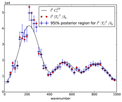
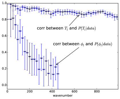
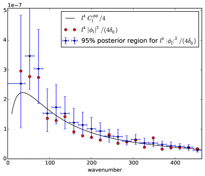
In Figures 8 and 9 we summarize the posterior draws for ϕitalic-ϕ\phi and T𝑇T in the Fourier domain. The left plot of Figure 8 shows 95%percent9595\% posterior regions for l4|ϕl|2/(4δ0)superscript𝑙4superscriptsubscriptitalic-ϕ𝑙24subscript𝛿0l^{4}|\phi_{l}|^{2}/(4\delta_{0}) averaged over l𝑙l in wavenumber bins. For comparison the simulation true values of l4|ϕl|2/(4δ0)superscript𝑙4superscriptsubscriptitalic-ϕ𝑙24subscript𝛿0l^{4}|\phi_{l}|^{2}/(4\delta_{0}) are shown in red and the spectral density l4Clϕϕ/4superscript𝑙4subscriptsuperscript𝐶italic-ϕitalic-ϕ𝑙4l^{4}C^{\phi\phi}_{l}/4 is plotted in the black solid line. The same quantities are shown for l2|Tl|2/(δ0)superscript𝑙2superscriptsubscript𝑇𝑙2subscript𝛿0l^{2}|T_{l}|^{2}/(\delta_{0}) in the right plot of Figure 8. Finally, in Figure 9 we show the empirical cross correlation of the posterior draws over wavenumber bins between the simulation truth and the posterior samples of ϕlsubscriptitalic-ϕ𝑙\phi_{l} and Tlsubscript𝑇𝑙T_{l}. In particular, samples were generated from 1clΔlϕlsimϕl1𝑐subscript𝑙Δ𝑙subscriptsuperscriptitalic-ϕsim𝑙subscriptsuperscriptitalic-ϕ𝑙\frac{1}{c}\sum_{l\in\Delta l}\phi^{\text{sim}}_{l}\phi^{*}_{l} and 1clΔlTlsimTl1𝑐subscript𝑙Δ𝑙subscriptsuperscript𝑇sim𝑙subscriptsuperscript𝑇𝑙\frac{1}{c}\sum_{l\in\Delta l}T^{\text{sim}}_{l}T^{*}_{l} where ΔlΔ𝑙\Delta l is a frequency wavenumber bin, ϕlsubscriptitalic-ϕ𝑙\phi_{l} and Tlsubscript𝑇𝑙T_{l} are the simulation truth, ϕlsimsubscriptsuperscriptitalic-ϕsim𝑙\phi^{\text{sim}}_{l} and Tlsimsubscriptsuperscript𝑇sim𝑙T^{\text{sim}}_{l} are sampled from the Gibbs algorithm presented here and c𝑐c is a normalization constant which transforms to a correlation scale. Notice that the plotted correlations trend to 00 for larger wavenumber. This is what one would expect since larger wavenumber have correspondingly less information which causes the posterior to revert back to the prior.

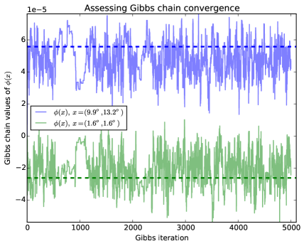
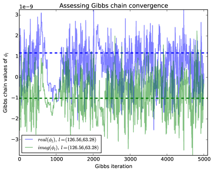
In Figure 10 we show the Gibbs chain correlation length scale and the speed of mixing for different statistics of the lensing potential. The left plot shows the Gibbs chain for ϕ(x)italic-ϕ𝑥\phi(x) where x=(9.9o,13.2o)𝑥superscript9.9𝑜superscript13.2𝑜x=(9.9^{o},13.2^{o}) and x=(1.6o,1.6o)𝑥superscript1.6𝑜superscript1.6𝑜x=(1.6^{o},1.6^{o}) in the same degree coordinates given in Figures 6 and 5. The right plot shows the real and imaginary parts of ϕlsubscriptitalic-ϕ𝑙\phi_{l} where the frequency vector l𝑙l is set to (126.56,63.28)126.5663.28(126.56,63.28). Each dashed line represents the corresponding simulation truth parameters. These plots suggest that the Gibbs chain is mixing well and that the correlation length scale is small enough so that thinning by 100100100 is sufficient to yield relatively uncorrelated samples.
Refer to caption
Refer to caption
Figure 8.— Estimates of l4|ϕl|2/4superscript𝑙4superscriptsubscriptitalic-ϕ𝑙24l^{4}|\phi_{l}|^{2}/4 and l2|Tl|2superscript𝑙2superscriptsubscript𝑇𝑙2l^{2}|T_{l}|^{2} (shown in blue), scaled to the units of the corresponding spectral density. The red dots show l4|ϕl|2/4superscript𝑙4superscriptsubscriptitalic-ϕ𝑙24l^{4}|\phi_{l}|^{2}/4 and l2|Tl|2superscript𝑙2superscriptsubscript𝑇𝑙2l^{2}|T_{l}|^{2} for the simulation truth (similarly scaled). The discrepancy between the red dots and the spectral densities, shown in black, is exclusively due to cosmic variance. The confidence bars show 95%percent9595\% probability regions from the posterior distributions P(l4|ϕl|2/4|data)𝑃conditionalsuperscript𝑙4superscriptsubscriptitalic-ϕ𝑙24dataP(l^{4}|\phi_{l}|^{2}/4\,|\,\text{data}) and P(l2|Tl|2|data)𝑃conditionalsuperscript𝑙2superscriptsubscript𝑇𝑙2dataP(l^{2}|T_{l}|^{2}\,|\,\text{data}).
Refer to caption
Figure 9.— This plot summaries the correlation, in ΔlΔ𝑙\Delta l wavenumber bins, between the simulation truth and their corresponding posterior samples. In particular, samples were generated from 1clΔlϕlsimϕl1𝑐subscript𝑙Δ𝑙subscriptsuperscriptitalic-ϕsim𝑙subscriptsuperscriptitalic-ϕ𝑙\frac{1}{c}\sum_{l\in\Delta l}\phi^{\text{sim}}_{l}\phi^{*}_{l} and 1clΔlTlsimTl1𝑐subscript𝑙Δ𝑙subscriptsuperscript𝑇sim𝑙subscriptsuperscript𝑇𝑙\frac{1}{c}\sum_{l\in\Delta l}T^{\text{sim}}_{l}T^{*}_{l} where ΔlΔ𝑙\Delta l is a frequency wavenumber bin, ϕlsubscriptitalic-ϕ𝑙\phi_{l} and Tlsubscript𝑇𝑙T_{l} are the simulation truth, ϕlsimsubscriptsuperscriptitalic-ϕsim𝑙\phi^{\text{sim}}_{l} and Tlsimsubscriptsuperscript𝑇sim𝑙T^{\text{sim}}_{l} is sampled from the Gibbs algorithm presented here and c𝑐c is a normalization constant which transforms to a correlation scale. Recall that |l|maxsubscript𝑙max|l|_{\text{max}} for the lensing potential is 460similar-toabsent460\sim 460 and is 2700similar-toabsent2700\sim 2700 for the unlensed CMB, which explains why the correlation for ϕlsubscriptitalic-ϕ𝑙\phi_{l} only extends to 460460460. Notice that the plotted correlations trend to 00 for larger wavenumber. This is what one would expect from the Bayesian posterior. Indeed, the data is less informative at larger wavenumber. This causes the Bayesian posterior to revert to the prior, which will be uncorrelated with the simulation truth.
Refer to caption
Refer to caption
Figure 10.— This plot illustrates the Gibbs chain correlation length scale and the speed of mixing for different statistics of the lensing potential. The left plot shows the Gibbs chain for ϕ(x)italic-ϕ𝑥\phi(x) where x=(9.9o,13.2o)𝑥superscript9.9𝑜superscript13.2𝑜x=(9.9^{o},13.2^{o}) and x=(1.6o,1.6o)𝑥superscript1.6𝑜superscript1.6𝑜x=(1.6^{o},1.6^{o}) in the same degree coordinates given in Figures 6 and 5. The right plot shows the real and imaginary parts of ϕlsubscriptitalic-ϕ𝑙\phi_{l} where the frequency vector l𝑙l is set to (126.56,63.28)126.5663.28(126.56,63.28). Each dashed line represents the corresponding simulation truth parameters. Recall that the algorithm is initialized with a zero lensing potential.

VIII. Concluding remarks

In this paper we construct a prototype algorithm which establishes that it is possible to construct a fast Gibbs sampler of the Bayesian posterior for the unknown lensing potential and the de-noised CMB temperature map. This prototype solves one of the fundamental obstacles in a Gibbs implementation of the Bayesian lensing problem: the naive parameterization (T,ϕ)𝑇italic-ϕ(T,\phi) is extremely slow. We identify the ancillary and sufficient parametrization duality for this problem and notice that the slowness of the Gibbs chain for the ancillary parametrization (T,ϕ)𝑇italic-ϕ(T,\phi) translates to a fast chain for the sufficient parametrization (T~,ϕ)~𝑇italic-ϕ(\widetilde{T},\phi). This observation is one of the main contributions of this paper. The second contribution is the use of the anti-lensing approximation along with Claim 1 which makes feasible the development of a Hamiltonian Markov Chain algorithm for sampling from P(ϕ|T~)𝑃conditionalitalic-ϕ~𝑇P(\phi|\widetilde{T}). Without the Fourier transform characterization in Claim 1 the HMC would be computational prohibitive. The third contribution of this paper is to recognize that a new messenger algorithm Elsner and Wandelt (2013); Jasche and Lavaux (2015) can be adapted for high resolution conditional Gaussian sampling under the irregular sampling scenario needed for P(T~|ϕ,data)𝑃conditional~𝑇italic-ϕdataP(\widetilde{T}|\phi,\text{data}).

Notice that both sampling steps P(ϕ|T~)𝑃conditionalitalic-ϕ~𝑇P(\phi|\widetilde{T}) and P(T~|ϕ,data)𝑃conditional~𝑇italic-ϕdataP(\widetilde{T}|\phi,\text{data}) in our algorithm utilize a high resolution embedding for T~~𝑇\widetilde{T}. This high resolution embedding is most likely the dominant bottleneck for scaling the current prototype implementation presented here. In this paragraph we discuss what is needed to avoid using this embedding for scaling up this algorithm. When sampling from the conditional P(ϕ|T~)𝑃conditionalitalic-ϕ~𝑇P(\phi|\widetilde{T}), the main challenge is to compute Aq(x)superscript𝐴𝑞𝑥A^{q}(x) and B(x)𝐵𝑥B(x), as defined in Claim 1. Within the HMC algorithm, a proposed lensing potential ϕitalic-ϕ\phi changes iteratively. A each iteration one requires a new computation of Aq(x)superscript𝐴𝑞𝑥A^{q}(x) and B(x)𝐵𝑥B(x). In our prototype, a spline interpolation performs the task of fast anti-lensing required for Aq(x)superscript𝐴𝑞𝑥A^{q}(x) and B(x)𝐵𝑥B(x). It is an open problem how to compute this fast anti-lensing without the need for a high resolution T~~𝑇\widetilde{T}. Simulating from P(T~|ϕ,data)𝑃conditional~𝑇italic-ϕdataP(\widetilde{T}|\phi,\text{data}) also requires a high resolution embedding in our prototype. This simply expresses the fact that given ϕitalic-ϕ\phi the field T~~𝑇\widetilde{T} is modeled as a non-stationary random field. To circumvent this difficulty we transform to lensed coordinates as illustrated in Figure 3. The challenge when avoiding this high resolution embedding, then, is to directly generate conditional simulations of the non-stationary T~~𝑇\widetilde{T} given data(x)=T~(x)+n(x)data𝑥~𝑇𝑥𝑛𝑥\text{data}(x)=\widetilde{T}(x)+n(x) and the lensing potential ϕ(x)italic-ϕ𝑥\phi(x).

Acknowledgments

BW acknowledges funding through his Chaire dÕExcellence from the Agence Nationale de la Recherche (ANR-10-CEXC-004-01). This work has been done within the Labex ILP (reference ANR-10-LABX-63) part of the Idex SUPER, and received financial state aid managed by the Agence Nationale de la Recherche, as part of the programme Investissements d’avenir under the reference ANR-11-IDEX-0004-02. EA acknowledges grant support from NSF CAREER DMS-1252795.

References

  • Das et al. (2011) S. Das et al., Physical Review Letters 107, 021301 (2011).
  • Engelen et al. (2012) V. Engelen et al., The Astrophysical Journal 756, 142 (2012).
  • Planck Collaboration (2014) Planck Collaboration, A&A 571, A17 (2014), eprint 1303.5077.
  • The Polarbear Collaboration: P. A. R. Ade et al. (2014) The Polarbear Collaboration: P. A. R. Ade, Y. Akiba, A. E. Anthony, K. Arnold, M. Atlas, D. Barron, D. Boettger, J. Borrill, S. Chapman, Y. Chinone, et al., ApJ 794, 171 (2014), eprint 1403.2369.
  • Planck Collaboration (2015) Planck Collaboration, ArXiv e-prints (2015), eprint 1502.01591.
  • Hu (2001) W. Hu, The Astrophysical Journal Letters 557, L79 (2001).
  • Hu and Okamoto (2002) W. Hu and T. Okamoto, The Astrophysical Journal 574, 566 (2002).
  • Hirata and Seljak (2003a) C. M. Hirata and U. c. v. Seljak, Phys. Rev. D 67, 043001 (2003a), URL http://link.aps.org/doi/10.1103/PhysRevD.67.043001.
  • Hirata and Seljak (2003b) C. M. Hirata and U. c. v. Seljak, Phys. Rev. D 68, 083002 (2003b), URL http://link.aps.org/doi/10.1103/PhysRevD.68.083002.
  • Lewis and Challinor (2006) A. Lewis and A. Challinor, Physics Reports 429, 1 (2006), ISSN 0370-1573, URL http://www.sciencedirect.com/science/article/pii/S0370157306000810.
  • Bezanson et al. (2012) J. Bezanson, S. Karpinski, V. Shah, and A. Edelman, arXiv preprint arXiv:1209.5145 (2012).
  • Dodelson (2003) S. Dodelson, Modern cosmology (Academic press, 2003).
  • Roberts et al. (2003) G. Roberts, O. Papaspiliopoulos, and M. Sköld, in Bayesian Statistics 7: Proceedings of the Seventh Valencia International Meeting (Oxford University Press, USA, 2003), p. 307.
  • Gelfand et al. (1995) A. Gelfand, S. Sahu, and B. Carlin, Biometrika 82, 479 (1995).
  • Papaspiliopoulos and Roberts (2008) O. Papaspiliopoulos and G. Roberts, The Annals of Statistics pp. 95–117 (2008).
  • Papaspiliopoulos et al. (2007) O. Papaspiliopoulos, G. Roberts, and M. Sköld, Statistical Science pp. 59–73 (2007).
  • Yu and Meng (2011) Y. Yu and X.-L. Meng, Journal of Computational and Graphical Statistics 20, 531 (2011).
  • Elsner and Wandelt (2013) F. Elsner and B. D. Wandelt, A&A 549, A111 (2013), eprint 1210.4931.
  • Jasche and Lavaux (2015) J. Jasche and G. Lavaux, MNRAS 447, 1204 (2015), eprint 1402.1763.
  • Neal (2011) R. M. Neal, Handbook of Markov Chain Monte Carlo 2 (2011).
  • Hajian (2007) A. Hajian, Phys. Rev. D 75, 083525 (2007), URL http://link.aps.org/doi/10.1103/PhysRevD.75.083525.
  • Taylor et al. (2008) J. F. Taylor, M. A. J. Ashdown, and M. P. Hobson, Monthly Notices of the Royal Astronomical Society 389, 1284 (2008).
  • Elsner and Wandelt (2010) F. Elsner and B. Wandelt, The Astrophysical Journal 724, 1262 (2010).
  • Jasche et al. (2010) J. Jasche, F. S. Kitaura, C. Li, and T. A. Enßlin, Monthly Notices of the Royal Astronomical Society 409, 355 (2010), eprint 0911.2498.
  • Jasche and Wandelt (2012) J. Jasche and B. Wandelt, Monthly Notices of the Royal Astronomical Society 425, 1042 (2012), eprint 1106.2757.
  • Jasche and Wandelt (2013a) J. Jasche and B. Wandelt, Monthly Notices of the Royal Astronomical Society p. stt449 (2013a).
  • Jasche and Wandelt (2013b) J. Jasche and B. Wandelt, The Astrophysical Journal 779, 15 (2013b).
  • Wandelt et al. (2004) B. D. Wandelt, D. L. Larson, and A. Lakshminarayanan, Phys. Rev. D 70, 083511 (2004), eprint astro-ph/0310080.
  • Eriksen et al. (2004) H. K. Eriksen, I. J. O’Dwyer, J. B. Jewell, B. D. Wandelt, D. L. Larson, K. M. Górski, S. Levin, A. J. Banday, and P. B. Lilje, ApJS 155, 227 (2004), eprint astro-ph/0407028.
  • Smith et al. (2007) K. M. Smith, O. Zahn, and O. Doré, Phys. Rev. D 76, 043510 (2007), eprint 0705.3980.
  • Seljebotn et al. (2014) D. S. Seljebotn, K.-A. Mardal, J. B. Jewell, H. K. Eriksen, and P. Bull, ApJS 210, 24 (2014), eprint 1308.5299.

Before we proceed to the proofs we briefly discuss notation. First, we do not differentiate, notationally, a random field with periodic boundary conditions on (L/2,L/2]2superscript𝐿2𝐿22(-L/2,L/2]^{2} and the case where L𝐿L\rightarrow\infty so that the Fourier series l2πLeixlfl2π/L2πsubscript𝑙2𝜋𝐿superscript𝑒𝑖𝑥𝑙subscript𝑓𝑙2𝜋𝐿2𝜋\sum_{l\in\frac{2\pi}{L}\mathbb{Z}}e^{ix\cdot l}f_{l}\frac{2\pi/L}{2\pi} converges to the continuous Fourier transform 2eixlfldl2πsubscriptsuperscript2superscript𝑒𝑖𝑥𝑙subscript𝑓𝑙𝑑𝑙2𝜋\int_{\mathbb{R}^{2}}e^{ix\cdot l}f_{l}\frac{dl}{2\pi}. For example, at times we will refer to an infinitesimal area element dl𝑑𝑙dl or dk𝑑𝑘dk in Fourier space, which simply equals (2π/L)2superscript2𝜋𝐿2(2\pi/L)^{2} for large L𝐿L. In this case, δlsubscript𝛿𝑙\delta_{l} denotes a discrete dirac delta function which we equate with 1/dl1𝑑𝑙1/dl when l=0𝑙0l=0 and zero otherwise. Secondly, for any function f(x)𝑓𝑥f(x) let fϕ(x)=f(xϕ(x))superscript𝑓italic-ϕ𝑥𝑓𝑥italic-ϕ𝑥f^{\phi}(x)=f(x-\nabla\phi(x)) denote anti-lensing of f𝑓f and flϕsubscriptsuperscript𝑓italic-ϕ𝑙f^{\phi}_{l} denote the Fourier transform of fϕ(x)superscript𝑓italic-ϕ𝑥f^{\phi}(x).

Proof of Claim 1.

Since T~~𝑇\widetilde{T} is sufficient for the unknown ϕitalic-ϕ\phi we have that

P(ϕ|T~,data)𝑃conditionalitalic-ϕ~𝑇data\displaystyle P(\phi|\widetilde{T},\text{\rm data}) =P(ϕ|T~)P(T~|ϕ)P(ϕ).absent𝑃conditionalitalic-ϕ~𝑇proportional-to𝑃conditional~𝑇italic-ϕ𝑃italic-ϕ\displaystyle=P(\phi|\widetilde{T})\propto P(\widetilde{T}|\phi)P(\phi).

Since ϕ(x)italic-ϕ𝑥\phi(x) is an isotropic random field with spectral density Clϕϕsuperscriptsubscript𝐶𝑙italic-ϕitalic-ϕC_{l}^{\phi\phi} we have that E(ϕlϕl)=δllClϕϕ𝐸subscriptsuperscriptitalic-ϕabsent𝑙superscriptsubscriptitalic-ϕsuperscript𝑙subscript𝛿𝑙superscript𝑙superscriptsubscript𝐶𝑙italic-ϕitalic-ϕE(\phi^{\phantom{*}}_{l}\phi_{l^{\prime}}^{*})=\delta_{l-l^{\prime}}C_{l}^{\phi\phi}. Therefore E(ϕlϕl)=δ0Clϕϕ𝐸superscriptsubscriptitalic-ϕ𝑙absentsuperscriptsubscriptitalic-ϕ𝑙subscript𝛿0superscriptsubscript𝐶𝑙italic-ϕitalic-ϕE(\phi_{l}^{\phantom{*}}\phi_{l}^{*})=\delta_{0}C_{l}^{\phi\phi} and E(ϕlϕl)=0𝐸subscriptitalic-ϕ𝑙subscriptitalic-ϕ𝑙0E(\phi_{l}\phi_{l})=0 implies that the random variables  reϕl resubscriptitalic-ϕ𝑙\text{\,\rm re}\phi_{l},  imϕl imsubscriptitalic-ϕ𝑙\text{\,\rm im}\phi_{l} are independent 𝒩(0,12δ0Clϕϕ)𝒩012subscript𝛿0superscriptsubscript𝐶𝑙italic-ϕitalic-ϕ\mathcal{N}(0,\frac{1}{2}\delta_{0}C_{l}^{\phi\phi}) for each fixed l𝑙l. Moreovoer ϕ(x)italic-ϕ𝑥\phi(x) takes values in \mathbb{R} so that ϕl=ϕlsubscriptitalic-ϕ𝑙superscriptsubscriptitalic-ϕ𝑙\phi_{l}=\phi_{-l}^{*}. This implies that ϕlsubscriptitalic-ϕ𝑙\phi_{l} and are independent random variables over all l𝑙l which are restricted to the Hermitian half of the Fourier grid, denoted \mathbb{H} here. In particular, if we exclude the zero frequency l=0𝑙0l=0 we get

logP(ϕ)c1𝑃italic-ϕsubscript𝑐1\displaystyle\log P(\phi)-c_{1} =12k{0}[( reϕk)212δ0Ckϕϕ+( imϕk)212δ0Ckϕϕ]=122|ϕk|2Ckϕϕ𝑑kabsent12subscript𝑘0delimited-[]superscript resubscriptitalic-ϕ𝑘212subscript𝛿0superscriptsubscript𝐶𝑘italic-ϕitalic-ϕsuperscript imsubscriptitalic-ϕ𝑘212subscript𝛿0superscriptsubscript𝐶𝑘italic-ϕitalic-ϕ12subscriptsuperscript2superscriptsubscriptitalic-ϕ𝑘2superscriptsubscript𝐶𝑘italic-ϕitalic-ϕdifferential-d𝑘\displaystyle=-\frac{1}{2}\sum_{k\in\mathbb{H}\setminus\{0\}}\left[\frac{(\text{\,\rm re}\phi_{k})^{2}}{\frac{1}{2}\delta_{0}C_{k}^{\phi\phi}}+\frac{(\text{\,\rm im}\phi_{k})^{2}}{\frac{1}{2}\delta_{0}C_{k}^{\phi\phi}}\right]=-\frac{1}{2}\int_{\mathbb{R}^{2}}\frac{|\phi_{k}|^{2}}{C_{k}^{\phi\phi}}dk (1)
logP(T~|ϕ)c2𝑃conditional~𝑇italic-ϕsubscript𝑐2\displaystyle\log P(\widetilde{T}|\phi)-c_{2} =12k{0}[( reT~kϕ)212δ0CkTT+( imT~kϕ)212δ0CkTT]=122|T~kϕ|2CkTT𝑑kabsent12subscript𝑘0delimited-[]superscript resuperscriptsubscript~𝑇𝑘italic-ϕ212subscript𝛿0superscriptsubscript𝐶𝑘𝑇𝑇superscript imsuperscriptsubscript~𝑇𝑘italic-ϕ212subscript𝛿0superscriptsubscript𝐶𝑘𝑇𝑇12subscriptsuperscript2superscriptsuperscriptsubscript~𝑇𝑘italic-ϕ2superscriptsubscript𝐶𝑘𝑇𝑇differential-d𝑘\displaystyle=-\frac{1}{2}\sum_{k\in\mathbb{H}\setminus\{0\}}\left[\frac{(\text{\,\rm re}\widetilde{T}_{k}^{\phi})^{2}}{\frac{1}{2}\delta_{0}C_{k}^{TT}}+\frac{(\text{\,\rm im}\widetilde{T}_{k}^{\phi})^{2}}{\frac{1}{2}\delta_{0}C_{k}^{TT}}\right]=-\frac{1}{2}\int_{\mathbb{R}^{2}}\frac{\bigl{|}\widetilde{T}_{k}^{\phi}\bigr{|}^{2}}{C_{k}^{TT}}dk (2)

where c1subscript𝑐1c_{1} and c2subscript𝑐2c_{2} are constants and T~ϕ(x)T~(xϕ(x))superscript~𝑇italic-ϕ𝑥~𝑇𝑥italic-ϕ𝑥\widetilde{T}^{\phi}(x)\equiv\widetilde{T}(x-\nabla\phi(x)).

Taking derivatives in (1) gives

ϕllogP(ϕ)=2(dl)ϕlClϕϕ.subscriptitalic-ϕ𝑙𝑃italic-ϕ2𝑑𝑙subscriptitalic-ϕ𝑙subscriptsuperscript𝐶italic-ϕitalic-ϕ𝑙\frac{\partial}{\partial\phi_{l}}\log P(\phi)=-2(dl)\frac{\phi_{l}}{C^{\phi\phi}_{l}}. (3)

Taking derivatives in (2) gives

 reϕllogP(T~|ϕ) resubscriptitalic-ϕ𝑙𝑃conditional~𝑇italic-ϕ\displaystyle\frac{\partial}{\partial\text{\,\rm re}\phi_{l}}\log P(\widetilde{T}|\phi) = re2T~kϕ reϕlT~kϕCkTT𝑑kabsent resubscriptsuperscript2superscriptsubscript~𝑇𝑘italic-ϕ resubscriptitalic-ϕ𝑙superscriptsubscript~𝑇𝑘superscriptitalic-ϕsuperscriptsubscript𝐶𝑘𝑇𝑇differential-d𝑘\displaystyle=-\text{\,\rm re}\int_{\mathbb{R}^{2}}\frac{\partial\widetilde{T}_{k}^{\phi}}{\partial\text{\,\rm re}\phi_{l}}\,\frac{\widetilde{T}_{k}^{\phi^{*}}}{C_{k}^{TT}}\,dk (4)
 imϕllogP(T~|ϕ) imsubscriptitalic-ϕ𝑙𝑃conditional~𝑇italic-ϕ\displaystyle\frac{\partial}{\partial\text{\,\rm im}\phi_{l}}\log P(\widetilde{T}|\phi) = re2T~kϕ imϕlT~kϕCkTT𝑑k.absent resubscriptsuperscript2superscriptsubscript~𝑇𝑘italic-ϕ imsubscriptitalic-ϕ𝑙superscriptsubscript~𝑇𝑘superscriptitalic-ϕsuperscriptsubscript𝐶𝑘𝑇𝑇differential-d𝑘\displaystyle=-\text{\,\rm re}\int_{\mathbb{R}^{2}}\frac{\partial\widetilde{T}_{k}^{\phi}}{\partial\text{\,\rm im}\phi_{l}}\,\frac{\widetilde{T}_{k}^{\phi^{*}}}{C_{k}^{TT}}\,dk. (5)

Taking linear combinations of the two equalities in Lemma 1 below we get

T~kϕ reϕlsubscriptsuperscript~𝑇italic-ϕ𝑘 resubscriptitalic-ϕ𝑙\displaystyle\frac{\partial\widetilde{T}^{\phi}_{k}}{\partial\text{\,\rm re}\phi_{l}} =12T~kϕϕl+12T~kϕϕl=dk2πq=1,2ilq{[(qT~)ϕ]kl[(qT~)ϕ]k+l}absent12subscriptsuperscript~𝑇italic-ϕ𝑘subscriptitalic-ϕ𝑙12subscriptsuperscript~𝑇italic-ϕ𝑘subscriptsuperscriptitalic-ϕ𝑙𝑑𝑘2𝜋subscript𝑞12𝑖subscript𝑙𝑞subscriptdelimited-[]superscriptsuperscript𝑞~𝑇italic-ϕ𝑘𝑙subscriptdelimited-[]superscriptsuperscript𝑞~𝑇italic-ϕ𝑘𝑙\displaystyle=\frac{1}{2}\frac{\partial\widetilde{T}^{\phi}_{k}}{\partial\phi_{l}}+\frac{1}{2}\frac{\partial\widetilde{T}^{\phi}_{k}}{\partial\phi^{*}_{l}}=\frac{dk}{2\pi}\sum_{q=1,2}il_{q}\left\{[(\nabla^{q}\widetilde{T})^{\phi}]_{k-l}-[(\nabla^{q}\widetilde{T})^{\phi}]_{k+l}\right\} (6)
T~kϕ imϕlsubscriptsuperscript~𝑇italic-ϕ𝑘 imsubscriptitalic-ϕ𝑙\displaystyle\frac{\partial\widetilde{T}^{\phi}_{k}}{\partial\text{\,\rm im}\phi_{l}} =i2T~kϕϕl+i2T~kϕϕl=dk2πq=1,2lq{[(qT~)ϕ]kl[(qT~)ϕ]k+l}.absent𝑖2subscriptsuperscript~𝑇italic-ϕ𝑘subscriptitalic-ϕ𝑙𝑖2subscriptsuperscript~𝑇italic-ϕ𝑘subscriptsuperscriptitalic-ϕ𝑙𝑑𝑘2𝜋subscript𝑞12subscript𝑙𝑞subscriptdelimited-[]superscriptsuperscript𝑞~𝑇italic-ϕ𝑘𝑙subscriptdelimited-[]superscriptsuperscript𝑞~𝑇italic-ϕ𝑘𝑙\displaystyle=\frac{-i}{2}\frac{\partial\widetilde{T}^{\phi}_{k}}{\partial\phi_{l}}+\frac{i}{2}\frac{\partial\widetilde{T}^{\phi}_{k}}{\partial\phi^{*}_{l}}=\frac{dk}{2\pi}\sum_{q=1,2}l_{q}\left\{-[(\nabla^{q}\widetilde{T})^{\phi}]_{k-l}-[(\nabla^{q}\widetilde{T})^{\phi}]_{k+l}\right\}. (7)

Now the above two equations establish, by Lemma 2 below, that both integrals 2T~kϕ reϕlT~kϕCkTT𝑑ksubscriptsuperscript2superscriptsubscript~𝑇𝑘italic-ϕ resubscriptitalic-ϕ𝑙superscriptsubscript~𝑇𝑘superscriptitalic-ϕsuperscriptsubscript𝐶𝑘𝑇𝑇differential-d𝑘\int_{\mathbb{R}^{2}}\frac{\partial\widetilde{T}_{k}^{\phi}}{\partial\text{\,\rm re}\phi_{l}}\,\frac{\widetilde{T}_{k}^{\phi^{*}}}{C_{k}^{TT}}\,dk and 2T~kϕ imϕlT~kϕCkTT𝑑ksubscriptsuperscript2superscriptsubscript~𝑇𝑘italic-ϕ imsubscriptitalic-ϕ𝑙superscriptsubscript~𝑇𝑘superscriptitalic-ϕsuperscriptsubscript𝐶𝑘𝑇𝑇differential-d𝑘\int_{\mathbb{R}^{2}}\frac{\partial\widetilde{T}_{k}^{\phi}}{\partial\text{\,\rm im}\phi_{l}}\,\frac{\widetilde{T}_{k}^{\phi^{*}}}{C_{k}^{TT}}\,dk are real which implies

ϕllogP(T~|ϕ)subscriptitalic-ϕ𝑙𝑃conditional~𝑇italic-ϕ\displaystyle\frac{\partial}{\partial\phi_{l}}\log P(\widetilde{T}|\phi) =2T~kϕϕlT~kϕCkTT𝑑kabsentsubscriptsuperscript2superscriptsubscript~𝑇𝑘italic-ϕsubscriptitalic-ϕ𝑙superscriptsubscript~𝑇𝑘superscriptitalic-ϕsuperscriptsubscript𝐶𝑘𝑇𝑇differential-d𝑘\displaystyle=-\int_{\mathbb{R}^{2}}\frac{\partial\widetilde{T}_{k}^{\phi}}{\partial\phi_{l}}\,\frac{\widetilde{T}_{k}^{\phi^{*}}}{C_{k}^{TT}}\,dk
=dkπq=1,2ilq2[(qT~)ϕ]k+lT~kϕCkTT𝑑kabsent𝑑𝑘𝜋subscript𝑞12𝑖subscript𝑙𝑞subscriptsuperscript2subscriptdelimited-[]superscriptsuperscript𝑞~𝑇italic-ϕ𝑘𝑙superscriptsubscript~𝑇𝑘superscriptitalic-ϕsuperscriptsubscript𝐶𝑘𝑇𝑇differential-d𝑘\displaystyle=-\frac{dk}{\pi}\sum_{q=1,2}il_{q}\int_{\mathbb{R}^{2}}[(\nabla^{q}\widetilde{T})^{\phi}]_{k+l}\,\frac{\widetilde{T}_{k}^{\phi^{*}}}{C_{k}^{TT}}\,dk
=i2(dk)q=1,2lq2[(qT~)ϕ]k+lT~kϕCkTTdk2πabsent𝑖2𝑑𝑘subscript𝑞12subscript𝑙𝑞subscriptsuperscript2subscriptdelimited-[]superscriptsuperscript𝑞~𝑇italic-ϕ𝑘𝑙superscriptsubscript~𝑇𝑘superscriptitalic-ϕsuperscriptsubscript𝐶𝑘𝑇𝑇𝑑𝑘2𝜋\displaystyle=-i2(dk)\sum_{q=1,2}l_{q}\int_{\mathbb{R}^{2}}[(\nabla^{q}\widetilde{T})^{\phi}]_{k+l}\,\frac{\widetilde{T}_{k}^{\phi^{*}}}{C_{k}^{TT}}\,\frac{dk}{2\pi}
=i2(dk)q=1,2lq2eixlAq(x)B(x)dx2π,by Lemma 3 belowabsent𝑖2𝑑𝑘subscript𝑞12subscript𝑙𝑞subscriptsuperscript2superscript𝑒𝑖𝑥𝑙superscript𝐴𝑞𝑥𝐵𝑥𝑑𝑥2𝜋by Lemma 3 below\displaystyle=-i2(dk)\sum_{q=1,2}l_{q}\int_{\mathbb{R}^{2}}e^{-ix\cdot l}A^{q}(x)\,B(x)\,\frac{dx}{2\pi},\quad\text{by Lemma \ref{conv} below}

where Aq(x)(qT~)ϕ(x)superscript𝐴𝑞𝑥superscriptsuperscript𝑞~𝑇italic-ϕ𝑥A^{q}(x)\equiv(\nabla^{q}\widetilde{T})^{\phi}(x) and Bk(T~kϕ)/CkTTsubscript𝐵𝑘superscriptsuperscriptsubscript~𝑇𝑘italic-ϕsuperscriptsubscript𝐶𝑘𝑇𝑇B_{k}\equiv(\widetilde{T}_{k}^{\phi})^{*}/C_{k}^{TT}. ∎

Lemma 1.
T~kϕϕlsubscriptsuperscript~𝑇italic-ϕ𝑘subscriptitalic-ϕ𝑙\displaystyle\frac{\partial\widetilde{T}^{\phi}_{k}}{\partial\phi_{l}} =dkπq=1,2ilq[(qT~)ϕ]k+labsent𝑑𝑘𝜋subscript𝑞12𝑖subscript𝑙𝑞subscriptdelimited-[]superscriptsuperscript𝑞~𝑇italic-ϕ𝑘𝑙\displaystyle=\frac{dk}{\pi}\sum_{q=1,2}\phantom{-}il_{q}[(\nabla^{q}\widetilde{T})^{\phi}]_{k+l} (8)
T~kϕϕlsubscriptsuperscript~𝑇italic-ϕ𝑘subscriptsuperscriptitalic-ϕ𝑙\displaystyle\frac{\partial\widetilde{T}^{\phi}_{k}}{\partial\phi^{*}_{l}} =dkπq=1,2ilq[(qT~)ϕ]klabsent𝑑𝑘𝜋subscript𝑞12𝑖subscript𝑙𝑞subscriptdelimited-[]superscriptsuperscript𝑞~𝑇italic-ϕ𝑘𝑙\displaystyle=\frac{dk}{\pi}\sum_{q=1,2}-il_{q}[(\nabla^{q}\widetilde{T})^{\phi}]_{k-l} (9)

where qT~T~xqsuperscript𝑞~𝑇~𝑇subscript𝑥𝑞\nabla^{q}\widetilde{T}\equiv\frac{\partial\widetilde{T}}{\partial x_{q}}.

Proof.

First notice

 reϕlϕ(x)xq resubscriptitalic-ϕ𝑙italic-ϕ𝑥subscript𝑥𝑞\displaystyle\frac{\partial}{\partial\text{\,\rm re}\phi_{l}}\frac{\partial\phi(x)}{\partial x_{q}} =2ikqeixkϕk reϕldk2π=[ilqeixlilqeixl]dk2πabsentsubscriptsuperscript2𝑖subscript𝑘𝑞superscript𝑒𝑖𝑥𝑘subscriptitalic-ϕ𝑘 resubscriptitalic-ϕ𝑙𝑑𝑘2𝜋delimited-[]𝑖subscript𝑙𝑞superscript𝑒𝑖𝑥𝑙𝑖subscript𝑙𝑞superscript𝑒𝑖𝑥𝑙𝑑𝑘2𝜋\displaystyle=\int_{\mathbb{R}^{2}}ik_{q}e^{ix\cdot k}\frac{\partial\phi_{k}}{\partial\text{\,\rm re}\phi_{l}}\frac{dk}{2\pi}=\left[il_{q}e^{ix\cdot l}-il_{q}e^{-ix\cdot l}\right]\frac{dk}{2\pi} (10)
 imϕlϕ(x)xq imsubscriptitalic-ϕ𝑙italic-ϕ𝑥subscript𝑥𝑞\displaystyle\frac{\partial}{\partial\text{\,\rm im}\phi_{l}}\frac{\partial\phi(x)}{\partial x_{q}} =2ikqeixkϕk imϕldk2π=[lqeixllqeixl]dk2π.absentsubscriptsuperscript2𝑖subscript𝑘𝑞superscript𝑒𝑖𝑥𝑘subscriptitalic-ϕ𝑘 imsubscriptitalic-ϕ𝑙𝑑𝑘2𝜋delimited-[]subscript𝑙𝑞superscript𝑒𝑖𝑥𝑙subscript𝑙𝑞superscript𝑒𝑖𝑥𝑙𝑑𝑘2𝜋\displaystyle=\int_{\mathbb{R}^{2}}ik_{q}e^{ix\cdot k}\frac{\partial\phi_{k}}{\partial\text{\,\rm im}\phi_{l}}\frac{dk}{2\pi}=\left[-l_{q}e^{ix\cdot l}-l_{q}e^{-ix\cdot l}\right]\frac{dk}{2\pi}. (11)

This implies

T~kϕϕlsubscriptsuperscript~𝑇italic-ϕ𝑘subscriptitalic-ϕ𝑙\displaystyle\frac{\partial\widetilde{T}^{\phi}_{k}}{\partial\phi_{l}} =ϕl2eixkT~(xϕ(x))dx2πabsentsubscriptitalic-ϕ𝑙subscriptsuperscript2superscript𝑒𝑖𝑥𝑘~𝑇𝑥italic-ϕ𝑥𝑑𝑥2𝜋\displaystyle=\frac{\partial}{\partial\phi_{l}}\int_{\mathbb{R}^{2}}e^{-ix\cdot k}\widetilde{T}(x-\nabla\phi(x))\frac{dx}{2\pi}
=q=1,22eixkqT~(xϕ(x))[ reϕlϕ(x)xqi imϕlϕ(x)xq]dx2πabsentsubscript𝑞12subscriptsuperscript2superscript𝑒𝑖𝑥𝑘superscript𝑞~𝑇𝑥italic-ϕ𝑥delimited-[] resubscriptitalic-ϕ𝑙italic-ϕ𝑥subscript𝑥𝑞𝑖 imsubscriptitalic-ϕ𝑙italic-ϕ𝑥subscript𝑥𝑞𝑑𝑥2𝜋\displaystyle=\sum_{q=1,2}\int_{\mathbb{R}^{2}}e^{-ix\cdot k}\nabla^{q}\widetilde{T}(x-\nabla\phi(x))\left[-\frac{\partial}{\partial\text{\,\rm re}\phi_{l}}\frac{\partial\phi(x)}{\partial x_{q}}-i\frac{\partial}{\partial\text{\,\rm im}\phi_{l}}\frac{\partial\phi(x)}{\partial x_{q}}\right]\frac{dx}{2\pi}
=q=1,2ilqdkπ2eix(k+l)qT~(xϕ(x))dx2π,by (10) and (11)absentsubscript𝑞12𝑖subscript𝑙𝑞𝑑𝑘𝜋subscriptsuperscript2superscript𝑒𝑖𝑥𝑘𝑙superscript𝑞~𝑇𝑥italic-ϕ𝑥𝑑𝑥2𝜋by (10) and (11)\displaystyle=\sum_{q=1,2}\frac{il_{q}dk}{\pi}\int_{\mathbb{R}^{2}}e^{-ix\cdot(k+l)}\nabla^{q}\widetilde{T}(x-\nabla\phi(x))\frac{dx}{2\pi},\quad\text{by (\ref{partial1}) and (\ref{partial2})}
=q=1,2ilqdkπ[(qT~)ϕ]k+labsentsubscript𝑞12𝑖subscript𝑙𝑞𝑑𝑘𝜋subscriptdelimited-[]superscriptsuperscript𝑞~𝑇italic-ϕ𝑘𝑙\displaystyle=\sum_{q=1,2}\frac{il_{q}dk}{\pi}[(\nabla^{q}\widetilde{T})^{\phi}]_{k+l} (12)

Similarly

T~kϕϕlsubscriptsuperscript~𝑇italic-ϕ𝑘subscriptsuperscriptitalic-ϕ𝑙\displaystyle\frac{\partial\widetilde{T}^{\phi}_{k}}{\partial\phi^{*}_{l}} =q=1,2ilqdkπ[(qT~)ϕ]kl.absentsubscript𝑞12𝑖subscript𝑙𝑞𝑑𝑘𝜋subscriptdelimited-[]superscriptsuperscript𝑞~𝑇italic-ϕ𝑘𝑙\displaystyle=\sum_{q=1,2}\frac{-il_{q}dk}{\pi}[(\nabla^{q}\widetilde{T})^{\phi}]_{k-l}. (13)

Lemma 2.

If A(x)𝐴𝑥A(x) and B(x)𝐵𝑥B(x) are real scalar fields then the two integrals, 2i{AklAk+l}Bk𝑑ksubscriptsuperscript2𝑖subscript𝐴𝑘𝑙subscript𝐴𝑘𝑙subscriptsuperscript𝐵𝑘differential-d𝑘\int_{\mathbb{R}^{2}}i\bigl{\{}A_{k-l}-A_{k+l}\bigr{\}}B^{*}_{k}dk and 2{Akl+Ak+l}Bk𝑑ksubscriptsuperscript2subscript𝐴𝑘𝑙subscript𝐴𝑘𝑙subscriptsuperscript𝐵𝑘differential-d𝑘\int_{\mathbb{R}^{2}}\bigl{\{}A_{k-l}+A_{k+l}\bigr{\}}B^{*}_{k}dk, are both real numbers.

Proof.

By a simple change of variables it is clear that 2(i{AklAk+l}Bk)𝑑k=2i{AklAk+l}Bk𝑑ksubscriptsuperscript2superscript𝑖subscript𝐴𝑘𝑙subscript𝐴𝑘𝑙subscriptsuperscript𝐵𝑘differential-d𝑘subscriptsuperscript2𝑖subscript𝐴superscript𝑘𝑙subscript𝐴superscript𝑘𝑙superscriptsubscript𝐵superscript𝑘differential-dsuperscript𝑘\int_{\mathbb{R}^{2}}\left(i\bigl{\{}A_{k-l}-A_{k+l}\bigr{\}}B^{*}_{k}\right)^{*}dk=\int_{\mathbb{R}^{2}}i\bigl{\{}A_{k^{\prime}-l}-A_{k^{\prime}+l}\bigr{\}}B_{k^{\prime}}^{*}dk^{\prime} and 2({Akl+Ak+l}Bk)𝑑k=2{Akl+Ak+l}Bk𝑑ksubscriptsuperscript2superscriptsubscript𝐴𝑘𝑙subscript𝐴𝑘𝑙subscriptsuperscript𝐵𝑘differential-d𝑘subscriptsuperscript2subscript𝐴superscript𝑘𝑙subscript𝐴superscript𝑘𝑙superscriptsubscript𝐵superscript𝑘differential-dsuperscript𝑘\int_{\mathbb{R}^{2}}\left(\bigl{\{}A_{k-l}+A_{k+l}\bigr{\}}B^{*}_{k}\right)^{*}dk=\int_{\mathbb{R}^{2}}\bigl{\{}A_{k^{\prime}-l}+A_{k^{\prime}+l}\bigr{\}}B_{k^{\prime}}^{*}dk^{\prime}.

The following lemma is equivalent to the so-called Convolution Theorem. We state it here for reference.

Lemma 3.

If A(x)𝐴𝑥A(x) and B(x)𝐵𝑥B(x) are real scalar fields then 2Ak+lBkdk2π=2eixlA(x)B(x)dx2πsubscriptsuperscript2subscript𝐴𝑘𝑙subscriptsuperscript𝐵𝑘𝑑𝑘2𝜋subscriptsuperscript2superscript𝑒𝑖𝑥𝑙𝐴𝑥𝐵𝑥𝑑𝑥2𝜋\int_{\mathbb{R}^{2}}A_{k+l}B^{*}_{k}\frac{dk}{2\pi}=\int_{\mathbb{R}^{2}}e^{-ix\cdot l}A(x)B(x)\frac{dx}{2\pi}.