Blind system identification
using kernel-based methods^⋆

Abstract

We propose a new method for blind system identification (BSI). Resorting to a Gaussian regression framework, we model the impulse response of the unknown linear system as a realization of a Gaussian process. The structure of the covariance matrix (or kernel) of such a process is given by the stable spline kernel, which has been recently introduced for system identification purposes and depends on an unknown hyperparameter. We assume that the input can be linearly described by few parameters. We estimate these parameters, together with the kernel hyperparameter and the noise variance, using an empirical Bayes approach. The related optimization problem is efficiently solved with a novel iterative scheme based on the Expectation-Maximization (EM) method. In particular, we show that each iteration consists of a set of simple update rules. We show, through some numerical experiments, very promising performance of the proposed method.

1 Introduction

In many engineering problems where data-driven modeling of dynamical systems is required, the experimenter may not have access to the input data. In these cases, standard system identification tools such as PEM [1] cannot be applied and specific methods, namely blind system identification (BSI) methods (or blind deconvolution, if one is mainly interested in the input), need be employed [2].

BSI finds applications in a wide range of engineering areas, such as image reconstruction [3], biomedical sciences  [4] and in particular communications [5, 6], for which literally hundreds of methods have been developed. It would be impossible to give a thorough literature review here.

Clearly, the unavailability of the input signal makes BSI problems generally ill-posed. Without further information on the input sequence or the structure of the system, it is impossible to retrieve a unique description of the system [7]. To circumvent (at least partially) this intrinsic non-uniqueness issue, we shall assume some prior knowledge on the input. Following the framework of [8] and [9], we describe the input sequence using a number of parameters considerably smaller than the length of the input sequence; see Section 2 for details and applications.

The main contribution of this paper is to propose a new BSI method. Our system modeling approach relies upon the kernel-based methods for linear system identification recently introduced in a series of papers [10, 11, 12, 13]. The main advantage of these methods, compared to standard parametric methods [1], is that the user is not required to select the model structure and order of the system, an operation that might be difficult if little is known about the dynamics of the system. Thus, we model the impulse response of the unknown system as a realization of a Gaussian random process, whose covariance matrix, or kernel, is given by the so called stable spline kernel [10, 14], which encodes prior information on BIBO stability and smoothness. Such a kernel depends on a hyperparameter which regulates the exponential decay of the generated impulse responses.

In the kernel-based framework, the estimate of the impulse response can be obtained as its Bayes estimate given the output data. However, when applied to BSI problems, such an estimator is a function of the kernel hyperparameter, the parameters characterizing the input and the noise variance. All these parameters need to be estimated from data. In this paper, using empirical Bayes arguments, we estimate such parameters by maximizing the marginal likelihood of the output measurements, obtained by integrating out the dependence on the system. In order to solve the related optimization problem, which is highly non-convex, involving a large number of variables, we propose a novel iterative solution scheme based on the Expectation-Maximization method [15]. We show that each iteration of such a scheme consists of a sequence of simple updates which can be performed using little computational efforts. Notably, our method is completely automatic, since the user is not required to tune any kind parameter. This in contrast with the BSI methods recently proposed in [8, 9], where, although the system is retrieved via a convex optimization problem, the user is required to select some regularization parameters and the model order. The method derived in this paper follows the same approach used in [16], where a novel method for Hammerstein system identification is described.

The paper is organized as follows. In the next section, we introduce the BSI problem and we state our working assumptions. In Section 3, we give a background on kernel-based methods, while in Section 4 we describe our approach to BSI. Section 5 presents some numerical experiments, and some conclusions end the paper.

2 Blind system identification

We consider a SISO linear time-invariant discrete-time dynamic system (see Figure 1)

$$y_{t}=\sum_{i=0}^{+\infty}g_{i}u_{t-i}+v_{t}\,,$$ (1)

where ${\{g_{t}\}}_{t=0}^{+\infty}$ is a strictly causal transfer function (i.e., $g_{0}=0$) representing the dynamics of the system, driven by the input $u_{t}$. The measurements of the output $y_{t}$ are corrupted by the process $v_{t}$, which is zero-mean white Gaussian noise with unknown variance $\sigma^{2}$. For the sake of simplicity, we will also hereby assume that the system is at rest until $t=0$.

Figure 1: Block scheme of the system identification scenario.

We assume that $N$ samples of the output measurements are collected, and denote them by ${\{y_{t}\}}_{t=1}^{N}$. The input $u(t)$ is not directly measurable and only some information about it is available. More specifically, we assume we know that the input, restricted to the $N$ time instants ${\{u_{t}\}}_{t=0}^{N-1}$, belongs to a certain subspace of $\mathbb{R}^{N}$ and thus can be written as

$$u=Hx\,,$$ (2)

where $u=\begin{bmatrix}u_{0}&\cdots&u_{N-1}\end{bmatrix}^{T}$. In the above equation, $H\in\mathbb{R}^{N\times p}$ is a known matrix with full column rank and $x\in\mathbb{R}^{p}$, $p\leq N$, is an unknown vector characterizing the evolution of $u(t)$. Below we report two examples of inputs generated in this way.

Piecewise constant inputs with known switching instants

Consider a piecewise constant input signal $u(t)$ with known switching instants $T_{1},T_{2}\dots T_{p}$, with $T_{p}=N$. The levels the input takes in between the switching instants are unknown and collected in the vector $x$. Then, the input signal can be expressed as

$$u=\begin{bmatrix}u_{0}\\ u_{1}\\ \vdots\\ u_{T_{1}-1}\\ u_{T_{1}}\\ \vdots\\ u_{T_{2}-1}\\ \vdots\\ u_{T_{p-1}}\\ \vdots\\ u_{T_{p}}\end{bmatrix}=\begin{bmatrix}1&&&\\ 1&&&\\ \vdots\\ 1&&&\\ &1&&\\ &\vdots&&\\ &1&&\\ &&\ddots&\\ &&&1\\ &&&\vdots\\ &&&1\end{bmatrix}\begin{bmatrix}x_{1}\\ x_{2}\\ \vdots\\ x_{p}\end{bmatrix}=Hx\,.$$ (3)

with

$$H=\mathrm{diag}\,\{\mathbf{1}_{T_{1}},\,\mathbf{1}_{T_{2}-T_{1}},\,\ldots,\,\mathbf{1}_{T_{p}-T_{p-1}}\}\,,H\in\mathbb{R}^{N\times p}$$ (4)

where $\mathbf{1}_{m}$ denotes a column vector of length $m$ with all entries equal to 1:

The vector $x$ needs to be estimated from output data. Applications of BSI with piecewise constant inputs are found in room occupancy estimation [17] and nonintrusive appliance load monitoring (NIALM) [18, 19].

Combination of known sinusoids

Assume that $u$ is composed by the sum of $p$ sinusoids with unknown amplitude and known frequencies $\omega_{1},\,\ldots,\,\omega_{p}$. Then in this case we have

$$H=\begin{bmatrix}\sin(\omega_{1})&\cdots&\sin(\omega_{p})\\ \vdots&&\vdots\\ \sin(N\omega_{1})&\cdots&\sin(N\omega_{p})\end{bmatrix}\,,$$ (5)

with $\omega_{1},\,\ldots,\,\omega_{p}$ such that $H$ is full column rank. The vector $x$ represents the amplitude of the sinusoids. Applications of this setting are found in blind channel estimation [9].

2.1 Problem statement

We state our BSI problem as the problem of obtaining an estimate of the impulse response $g_{t}$ for $n$ time instants, namely ${\{g_{t}\}}_{t=1}^{n}$, given ${\{y_{t}\}}_{t=1}^{N}$ and $H$. Recall that, by choosing $n$ sufficiently large, these samples can be used to approximate $g_{t}$ with arbitrary accuracy [1]. To achieve our goal we will need to estimate the input $u=\begin{bmatrix}u_{0}&\cdots&u_{N-1}\end{bmatrix}^{T}$; hence, we might also see our problem as a blind deconvolution problem.

Remark 1

The identification method we propose in this paper can be derived also in the continuous-time setting, using the same arguments as in [10]. However, for ease of exposition, here we focus only on the discrete-time case.

In a condition of complete information, this problem can be solved by least squares [1] or using regularized kernel-based approaches  [10], [11], [12].

2.2 Identifiability issues

It is well-known that BSI problems are not completely solvable (see e.g. [2, 5]). This because the system and the input can be determined up to a scaling factor, in the sense that every pair $(\alpha u,\frac{1}{\alpha}g)$, $\alpha\in\mathbb{R}$, can describe the output dynamics equally well. Hence, we shall consider our BSI problem as the problem of determining the system and the input up to a scaling factor. Another possible way out for this issue is to assume that $\|g\|_{2}$ or $g_{1}$ are known [20].

3 Kernel-based system identification

In this section we briefly review the kernel-based approach introduced in [10, 11] and show how to readapt it to BSI problem.

Let us first introduce the following vector notation

$$u:=\begin{bmatrix}u_{0}\\ \vdots\\ u_{N-1}\end{bmatrix}\,,y:=\begin{bmatrix}y_{1}\\ \vdots\\ y_{N}\end{bmatrix}\,,\,g:=\begin{bmatrix}g_{1}\\ \vdots\\ g_{n}\end{bmatrix},\,v:=\begin{bmatrix}v_{1}\\ \vdots\\ v_{N}\end{bmatrix}$$

and the operator $\mathbf{T}_{n}(\cdot)$ that, given a vector of length $N$, maps it to an $N\times n$ Toeplitz matrix, e.g.

$$\mathbf{T}_{n}(u)=\begin{bmatrix}u_{0}&0&&\cdots&0\\ u_{1}&u_{0}&0&\cdots&0\\ \vdots&\vdots&&\ddots&\vdots\\ u_{N-2}&u_{N-3}&\cdots&u_{N-n+1}&0\\ u_{N-1}&u_{N-2}&\cdots&\cdots&u_{N-n}\end{bmatrix}\,\in\,\mathbb{R}^{N\times n}\,.$$

We shall reserve the symbol $U$ for $\mathbf{T}_{n}(u)$. Then, the input-output relation for the available samples can be written

$$y=Ug+v\,.$$ (6)

In this paper we adopt a Bayesian approach to the BSI problem. Following a Gaussian process regression approach [21], we model the impulse response as follows

$$g\sim\mathcal{N}(0,\lambda K_{\beta})$$ (7)

where $K_{\beta}$ is a covariance matrix whose structure depends on a shaping parameter $\beta$, and $\lambda\geq 0$ is a scaling factor, which regulates the amplitude of the realizations from (7). Given the identifiability issue described in Section 2.2, $\lambda$ can be arbitrarily set to 1. In the context of Gaussian regression, $K_{\beta}$ is usually called a kernel and its structure is crucial in imposing properties on the realizations drawn from (7). An effective choice of kernel for system identification purposes is given by the so-called stable spline kernels [10, 11]. In particular, in this paper we adopt the so-called first-order stable spline kernel (or TC kernel in [12]), which is defined as

$${\{K_{\beta}\}}_{i,j}:=\beta^{\max(i,j)}\,,$$ (8)

where $\beta$ is a scalar in the interval $[0,\,1)$. Such a parameter regulates the decaying velocity of the generated impulse responses.

Recall the assumption introduced in Section 2 on the Gaussianity of noise. Due to this assumption, the joint distribution of the vectors $y$ and $g$ is Gaussian, provided that the vector $x$ (and hence the input $u$), the noise variance $\sigma^{2}$ and the parameter $\beta$ are given. Let us introduce the vector

$$\theta:=\begin{bmatrix}x^{T}&\sigma^{2}&\beta\end{bmatrix}\quad\in\mathbb{R}^{p+2}\,,$$ (9)

which we shall call hyperparameter vector. Then we can write

$$p\left(\left.\begin{bmatrix}y\\ g\end{bmatrix}\right|\theta\right)\sim\mathcal{N}\left(\begin{bmatrix}0\\ 0\end{bmatrix},\begin{bmatrix}\Sigma_{y}&\Sigma_{yg}\\ \Sigma_{gy}&K_{\beta}\end{bmatrix}\right)\,,$$ (10)

where $\Sigma_{yg}=\Sigma_{gy}^{T}=UK_{\beta}$ and $\Sigma_{y}=UK_{\beta}U^{T}+\sigma^{2}I$. It follows that the posterior distribution of $g$ given $y$ (and $\theta$) is Gaussian, namely

$$p(g|y,\,\theta)=\mathcal{N}\left(Cy,\,P\right)\,,$$ (11)

where

$$P={\left(\frac{U^{T}U}{\sigma^{2}}+K_{\beta}^{-1}\right)}^{-1}\quad,\quad C=P\frac{U^{T}}{\sigma^{2}}\,.$$ (12)

From (11), the impulse response estimator can be derived as the Bayesian estimator [22]

$$\hat{g}=\mathbb{E}[g|y,\,\theta]=Cy\,.$$ (13)

Clearly, such an estimator is a function of $\theta$, which needs to be determined from the available data $y$ before performing the estimation of $g$. Thus, the BSI algorithm we propose in this paper consists of the following steps.

1. Estimate the hyperparameter vector $\theta$.

2. Obtain $\hat{g}$ by means of (13).

In the next section, we discuss how to efficiently compute the first step of the algorithm.

4 Estimation of the hyperparameter vector

An effective approach to choose the hyperparameter vector characterizing the impulse response estimator (13) relies on Empirical Bayes arguments [23]. More precisely, since $y$ and $g$ are jointly Gaussian, an efficient method to choose $\theta$ is given by maximization of the marginal likelihood [24], which is obtained by integrating out $g$ from the joint probability density of $(y,\,g)$. Hence, an estimate of $\theta$ can be computed as follows

$$\hat{\theta}=\arg\max_{\theta}\log p(y|\theta)\,.$$ (14)

Solving (14) in that form can be hard, because it is a nonlinear and non-convex problem involving a large number ($p+2$) of decision variables. For this reason, we propose an iterative solution scheme which resorts to the EM method. To this end, we define the complete likelihood

$$L(y,\,g|\theta):=\log p(y,\,g|\theta)\,,$$ (15)

which depends also on the missing data $g$. Then, the EM method provides $\hat{\theta}$ by iterating the following steps:

(E-step)

Given an estimate $\hat{\theta}^{k}$ after the $k$-th iteration of the scheme, compute

$$\mathcal{Q}(\theta,\,\hat{\theta}^{k}):=\mathbb{E}_{p(g|y,\,\hat{\theta}^{k})}\left[L(y,\,g|\theta)\right]\,;$$ (16)

(M-step)

Compute

$$\hat{\theta}^{k+1}=\arg\max_{\theta}\mathcal{Q}(\theta,\,\hat{\theta}^{k})\,.$$ (17)

The iteration of these steps is guaranteed to converge to a (local or global) maximum of (14) [25], and the iterations can be stopped if $\|\hat{\theta}^{k+1}-\hat{\theta}^{k}\|_{2}$ is below a given threshold.

Assume that, at iteration $k+1$ of the EM scheme, the estimate $\hat{\theta}^{k}$ of $\theta$ is available. Using the current estimate of the hyperparameter vector, we construct the matrices $\hat{C}^{k}$ and $\hat{P}^{k}$ using (12) and, accordingly, we denote by $\hat{g}^{k}$ the estimate of $g$ computed using (13), i.e. $\hat{g}^{k}=\hat{C}^{k}y$ and the linear prediction of $y$ as $\hat{y}^{k}=U\hat{g}^{k}$. Furthermore, let us define

$$\hat{A}^{k} =-H^{T}\mathbf{R}^{T}\left((\hat{P}^{k}+\hat{g}^{k}\hat{g}^{kT})\otimes I_{N}\right)\mathbf{R}H$$

$$\hat{b}^{k} =H^{T}{\mathbf{T}_{N}(\hat{g}^{k})}^{T}y\,,$$ (18)

where $\mathbf{R}\in\mathbb{R}^{Nn\times N}$ is a matrix such that, for any $u\in\mathbb{R}^{N}$:

$$\mathbf{R}u=\mathrm{vec}(\mathbf{T}_{n}(u))\,.$$ (19)

Having introduced this notation, we can state the following theorem, which provides a set of upgrade rules to obtain the hyperparameter vector estimate $\hat{\theta}^{k+1}$.

Theorem 1

Let $\hat{\theta}^{k}$ be the estimate of the hyperparameter vector after the $k$-th iteration of the EM scheme. Then

$$\hat{\theta}^{k+1}=\begin{bmatrix}\hat{x}^{k+1,T}&\hat{\sigma}^{2,k+1}&\hat{\beta}^{k+1}\end{bmatrix}$$ (20)

can be obtained performing the following operations:

• The input estimate is updated computing

  $$\hat{x}^{k+1}=-{(A^{k})}^{-1}b^{k}\,;$$ (21)

• The noise variance is updated computing

  $$\hat{\sigma}^{2,k+1}=\frac{1}{N}\left(\|y-\hat{y}^{k}\|_{2}^{2}+\mathrm{Tr}\left[\hat{U}^{k+1}\hat{P}^{k}\hat{U}^{k+1,T}\right]\right)\,,$$ (22)

  where $\hat{U}^{k+1}$ denotes the Toeplitz matrix of the sequence $\hat{u}^{k+1}=H\hat{x}^{k+1}$;

• The kernel shaping parameter is updated solving

  $$\hat{\beta}^{k+1}=\arg\min_{\beta\in[0,\,1)}\mathcal{Q}(\beta,\hat{\theta}^{k})\,,$$ (23)

  where

  $$\!\!\!\mathcal{Q}(\beta,\hat{\theta}^{k})=\log\det K_{\beta}+\mathrm{Tr}\left[K_{\beta}^{-1}(\hat{P}^{k}+\hat{g}^{k}\hat{g}^{kT})\right].$$ (24)

Hence, the maximization problem (14) reduces to a sequence of very simple optimization problems. In fact, at each iteration of the EM algorithm, the input can be estimated by computing a simple update rule available in closed-form. The same holds for the noise variance, whereas the update of the kernel hyperparameter $\beta$ does not admit any closed-form expression. However, it can be retrieved by solving a very simple scalar optimization problem, which can be solved efficiently by grid search, since the domain of $\beta$ is the interval $[0,\,1)$.

It remains to establish a way to set up the initial estimate $\hat{\theta}^{0}$ for the EM method. This can be done by just randomly choosing the entries of such a vector, keeping the constraints $\hat{\beta}^{0}\in[0,\,1)$, $\hat{\sigma}^{2,0}>0$.

Below, we provide our BSI algorithm.

Algorithm: Bayesian kernel-based EM Blind System Identification
Input: ${\{y_{t}\}}_{t=1}^{N}$, $H$
Output: ${\{\hat{g}\}}_{t=1}^{n}$, ${\{\hat{u}_{t}\}}_{t=1}^{N}$

1. Initialization: randomly set $\hat{\theta}^{0}=\begin{bmatrix}\hat{x}^{0T}&\hat{\sigma}^{2,0}&\hat{\beta}^{0}\end{bmatrix}$

2. Repeat until convergence:

   1. E-step: update $\hat{P}^{k}$, $\hat{C}^{k}$ from (12) and $\hat{g}^{k}$ from (13);

   2. M-step: update the parameters:

      • $\hat{x}^{k+1}$ from (21);

      • $\hat{\sigma}^{k+1}$ from (22),

      • $\hat{\beta}^{k+1}$ from (23)

3. Compute ${\{\hat{g}\}}_{t=1}^{n}$ from (13) and ${\{\hat{u}_{t}\}}_{t=1}^{N}=H\hat{x}$;

5 Numerical experiments

We test the proposed BSI method by means of Monte Carlo experiments. Specifically, we perform 6 groups of simulations where, for each group, 100 random systems and input/output trajectories are generated. The random systems are generated by picking 20 zeros and 20 poles with random magnitude and phase. The zero magnitude is less than or equal to 0.95 and the pole magnitude is no larger than 0.92. The inputs are piecewise constant signals and the number of switching instants is $p=10,\,20,\,30,\,40,\,50,\,60$, depending on the group of experiments. We generate 200 input/output samples per experiment. The output is corrupted by random noise whose variance is such that $\sigma^{2}=\mathrm{var}(Ug)/10$, i.e. the noise variance is ten times smaller than the variance of the noiseless output. The goal of the experiments is to estimate $n=50$ samples of the generated impulse responses. We compare the following three estimators.

• B-KB. This is the proposed Bayesian kernel-based BSI method that estimates the input by marginal likelihood maximization, using an EM-based scheme. The convergence criterion of the EM method is $\|\hat{\theta}^{k+1}-\hat{\theta}^{k}\|_{2}<10^{-3}$.

• NB-LS. This is an impulse response estimator based on the least squares criterion. Here, we assume that the input is known, so the only quantity to be estimated is the system. Hence, this corresponds to an unbiased FIR estimator [1].

• NB-KB. This is the Bayesian kernel-based system identification method introduced in [10] and revisited in [12]. Like the estimator NB-LS, this method has knowledge of the input and in fact corresponds to the estimator B-KB when $x$ is known and not estimated.

The performance of the estimators are evaluated by means of the output fitting score

$$FIT=1-\frac{\|\hat{U}_{i}\hat{g}_{i}-U_{i}g_{i}\|_{2}}{\|U_{i}g_{i}-\overline{U_{i}g_{i}}\|_{2}}\,,$$ (25)

where, at the $i$-th Monte Carlo run, ${U}_{i}$ and $\hat{U}_{i}$ are the Toeplitz matrices of the true and estimated inputs ($\hat{U}_{i}={U}_{i}$ if the method needs not estimate $x$), ${g}_{i}$ and $\hat{g}_{i}$ are the true and estimated systems and $\overline{U_{i}g_{i}}$ is the mean of $U_{i}g_{i}$.

Figure 2 shows the results of the six group of experiments. As expected, the estimator NB-KB, which has access to the true input, gives the best performance for all the values of $p$ and in fact is independent of such a value. Surprisingly, for $p=10$ amd $p=20$, the proposed BSI method outperforms the least squares estimator that knows the true input. An example of one such Monte Carlo experiments in reported in Figure 3.

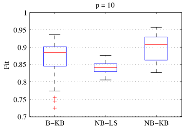
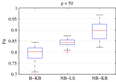
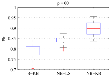
Figure 2: Results of the Monte Carlo simulations for different values of $p$, namely the number of different levels in the input signals.

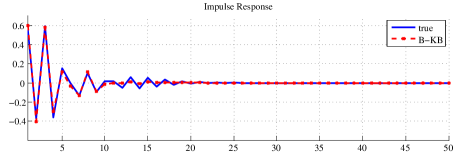
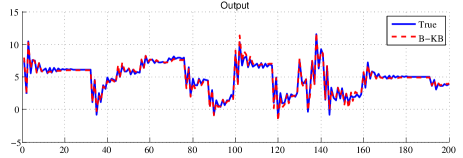
Figure 3: Example of one Monte Carlo realization with $p=20$. Top panel: true vs estimated (normalized) input. Middle panel: true vs estimated (normalized) impulse response. Bottom panel: true vs predicted output.

As one might expect, there is a performance degradation as $p$ increases, since the blind estimator has to estimate more parameters. Figure 4 shows the median of the fitting score of each group of experiments as function of $p$. It appears that, approximately, there is a linear trend in the performance degradation.

Figure 4: Median of the fitting score for each group of Monte Carlo simulations as function of $p$.

6 Conclusions

In this paper we have proposed a novel blind system identification algorithm. Under a Gaussian regression framework, we have modeled the impulse response of the unknown system as the realization of a Gaussian process. The kernel chosen to model the system is the stable spline kernel. We have assumed that the unknown input belongs to a known subspace of the input space. The estimation of the input, together with the kernel hyperparameter and the noise variance, has been performed using an empirical Bayes approach. We have solved the related maximization problem resorting to the EM method, obtaining a set of update rules for the parameters which is simple and elegant, and permits a fast computation of the estimates of the system and the input. We have shown, through some numerical experiments, very promising results.

We plan to extend the current method in two ways. First, a wider class of models of the system, such as the Box-Jenkins model, will be considered. We shall also attempt to remove the assumption on the input belonging to a known subspace by adopting suitable Bayesian models.

Appendix A Proof of Theorem 1

First note that $p(y,\,g|\theta)=p(y|g,\,\theta)p(g|\theta)$. Hence we can write the complete likelihood as

$$L(y,\,g|\theta)=\log p(y|g,\,\theta)+\log p(g|\theta)$$ (26)

and so

$$\begin{split}L(y,\,g|\theta)&=-\frac{N}{2}\log\sigma^{2}-\frac{1}{2\sigma^{2}}\left\|y-Ug\right\|^{2}\\ &\quad-\frac{1}{2}\log\det K_{\beta}-\frac{1}{2}g^{T}K_{\beta}^{-1}g\\ &=-\frac{N}{2}\log\sigma^{2}-\frac{1}{2\sigma^{2}}\left(y^{T}y+g^{T}U^{T}Ug-2y^{T}Ug\right)\\ &\quad-\frac{1}{2}\log\det K_{\beta}-\frac{1}{2}g^{T}K_{\beta}^{-1}g\,.\end{split}$$

We now proceed by taking the expectation of this expression with respect to the random variable $g|y,\hat{\theta}^{k}$. We obtain the following components

$$(a) :\mathbb{E}\left[-\frac{N}{2}\log\sigma^{2}\right]\!=\!-\frac{N}{2}\log\sigma^{2}\allowdisplaybreaks[1]$$

$$(b) :\mathbb{E}\left[-\frac{1}{2\sigma^{2}}y^{T}y\right]\!=\!-\frac{1}{2\sigma^{2}}y^{T}y\allowdisplaybreaks[1]$$

$$(c) :\mathbb{E}\left[-\frac{1}{2\sigma^{2}}g^{T}U^{T}Ug\right]\!=\!\mathrm{Tr}\left[-\frac{1}{2\sigma^{2}}U^{T}U(\hat{P}^{k}\!+\!\hat{g}^{k}\hat{g}^{kT})\right]\allowdisplaybreaks[1]$$

$$(d) :\mathbb{E}\left[\frac{1}{\sigma^{2}}y^{T}Ug\right]\!=\!\frac{1}{\sigma^{2}}y^{T}U\hat{g}^{k}\allowdisplaybreaks[1]$$

$$(e) :\mathbb{E}\left[-\frac{1}{2}\log\det K_{\beta}\right]\!=\!-\frac{1}{2}\log\det K_{\beta}\allowdisplaybreaks[1]$$

$$(f) :\mathbb{E}\left[-\frac{1}{2}g^{T}K_{\beta}^{-1}g\right]=-\frac{1}{2}\mathrm{Tr}\left[K_{\beta}^{-1}(\hat{P}^{k}+\hat{g}^{k}\hat{g}^{kT})\right]$$

It follows that $Q(\theta,\,\hat{\theta}^{k})$ is the summation of the elements obtained above. By inspecting the structure of $Q(\theta,\,\hat{\theta}^{k})$, it can be seen that such a function splits in two independent terms, namely

$$\mathcal{Q}(\theta,\,\hat{\theta}^{k})=\mathcal{Q}_{1}(x,\,\sigma^{2},\,\hat{\theta}^{k})+\mathcal{Q}_{\beta}(\beta,\,\hat{\theta}^{k})\,,$$ (27)

where

$$\mathcal{Q}_{1}(x,\,\sigma^{2},\,\hat{\theta}^{k})=(a)+(b)+(c)+(d)$$ (28)

is function of $x$ and $\sigma^{2}$, while

$$\mathcal{Q}_{\beta}(\beta,\,\hat{\theta}^{k})=(e)+(f)$$ (29)

depends only on $\beta$ and corresponds to (24). We now address the optimization of (28). To this end we write

$$\mathcal{Q}_{1}(x,\sigma^{2},\,\hat{\theta}^{k}) =\frac{1}{\sigma^{2}}\mathcal{Q}_{x}(x,\,\hat{\theta}^{k})+\mathcal{Q}_{\sigma^{2}}(\sigma^{2},\,\hat{\theta}^{k})$$ (30)

$$=\frac{1}{\sigma^{2}}\left(\mathrm{Tr}\left[-\frac{1}{2}U^{T}U(\hat{P}^{k}\!+\!\hat{g}^{k}\hat{g}^{kT})\right]+y^{T}U\hat{g}^{k}\right)$$

$$\quad-\frac{N}{2}\log\sigma^{2}-\frac{1}{2\sigma^{2}}y^{T}y\,.$$

This means that the optimization of $\mathcal{Q}_{1}$ can be carried out first with respect to $x$, optimizing only the term $\mathcal{Q}_{x}$, which is independent of $\sigma^{2}$ and can be written in a quadratic form

$$\mathcal{Q}_{x}(x,\,\hat{\theta}^{k})=\frac{1}{2}x^{T}\hat{A}^{k}x+\hat{b}^{kT}x\,.$$ (31)

To this end, first note that, for all $v_{1}\in\mathbb{R}^{n}$, $v_{2}\in\mathbb{R}^{m}$,

$$\mathbf{T}_{m}(v_{1})v_{2}=\mathbf{T}_{n}(v_{2})v_{1}\,.$$ (32)

Recalling (19), we can write

$$\mathrm{Tr}\left[U^{T}U(\hat{P}^{k}\!\!+\!\!\hat{g}^{k}\hat{g}^{kT})\right]\!\!=\!\!{\mathrm{vec}(U)}^{T}\!((\hat{P}^{k}\!\!+\!\!\hat{g}^{k}\hat{g}^{kT})\otimes I_{N})\mathrm{vec}(U)$$

$$=-\frac{1}{2}u^{T}\mathbf{R}^{T}\left((\hat{P}^{k}+\hat{g}^{k}\hat{g}^{kT})\otimes I_{N}\right)\mathbf{R}u$$ (33)

$$=-\frac{1}{2}x^{T}H^{T}\mathbf{R}^{T}\left((\hat{P}^{k}+\hat{g}^{k}\hat{g}^{kT})\otimes I_{N}\right)\mathbf{R}Hx\,,$$

where the matrix in the middle corresponds to $\hat{A}^{k}$ defined in (4). For the linear term we find

$$y^{T}U\hat{g}^{k}=y^{T}\mathbf{T}_{N}(\hat{g}^{k})u=y^{T}\mathbf{T}_{N}(\hat{g}^{k})Hx\,,$$ (34)

so that the term $\hat{b}^{kT}$ in (4) is retrieved and the maximizer $\hat{x}^{k+1}$ is as in (21). Plugging back $\hat{x}^{k+1}$ into (28) and maximizing with respect to $\sigma^{2}$ we easily find $\hat{\sigma}^{2,k+1}$ corresponding to (22). This concludes the proof.

References

- [1] L. Ljung “System Identification, Theory for the User” Prentice Hall, 1999
- [2] K. Abed-Meraim, W. Qiu and Y. Hua “Blind system identification” In Proc. IEEE 85.8, 1997, pp. 1310–1322 DOI: 10.1109/5.622507
- [3] G. R. Ayers and J. C. Dainty “Iterative blind deconvolution method and its applications” In Opt. Lett. 13.7, 1988, pp. 547 DOI: 10.1364/ol.13.000547
- [4] D. B. McCombie, A. T. Reisner and H. H. Asada “Laguerre-Model Blind System Identification: Cardiovascular Dynamics Estimated From Multiple Peripheral Circulatory Signals” In IEEE Trans. Biomed. Eng. 52.11, 2005, pp. 1889–1901 DOI: 10.1109/tbme.2005.856260
- [5] F. Gustafsson and B. Wahlberg “Blind equalization by direct examination of the input sequences” In IEEE Trans. Commun. 43.7, 1995, pp. 2213–2222 DOI: 10.1109/26.392964
- [6] E Moulines, P Duhamel, J-F Cardoso and S Mayrargue “Subspace methods for the blind identification of multichannel FIR filters” In IEEE Trans. Signal Process. 43.2 Institute of Electrical & Electronics Engineers (IEEE), 1995, pp. 516–525 DOI: 10.1109/78.348133
- [7] L Tong, R-W Liu, V C Soon and Y-F Huang “Indeterminacy and identifiability of blind identification” In IEEE Trans. Circuits Syst. 38.5, 1991, pp. 499–509 DOI: 10.1109/31.76486
- [8] H. Ohlsson, L. J. Ratliff, R. Dong and S. S. Sastry “Blind Identification Via Lifting” In Proc. IFAC World Cong., 2014 DOI: 10.3182/20140824-6-za-1003.02567
- [9] A. Ahmed, B. Recht and J. Romberg “Blind Deconvolution Using Convex Programming” In IEEE Trans. Inform. Theory 60.3, 2014, pp. 1711–1732 DOI: 10.1109/tit.2013.2294644
- [10] Gianluigi Pillonetto and Giuseppe De Nicolao “A new kernel-based approach for linear system identification” In Automatica 46.1 Elsevier, 2010, pp. 81–93 DOI: doi:10.1016/j.automatica.2009.10.031
- [11] Gianluigi Pillonetto, Alessandro Chiuso and Giuseppe De Nicolao “Prediction error identification of linear systems: a nonparametric Gaussian regression approach” In Automatica 47.2 Elsevier, 2011, pp. 291–305 DOI: 10.1016/j.automatica.2010.11.004
- [12] T. Chen, H. Ohlsson and L. Ljung “On the estimation of transfer functions, regularizations and Gaussian processes—Revisited” In Automatica 48.8 Elsevier, 2012, pp. 1525–1535 DOI: 10.1016/j.automatica.2012.05.026
- [13] Gianluigi Pillonetto, Francesco Dinuzzo, Tianshi Chen, Giuseppe De Nicolao and Lennart Ljung “Kernel methods in system identification, machine learning and function estimation: A survey” In Automatica 50.3 Elsevier BV, 2014, pp. 657–682 DOI: 10.1016/j.automatica.2014.01.001
- [14] G. Bottegal and G. Pillonetto “Regularized spectrum estimation using stable spline kernels” In Automatica 49.11 Elsevier, 2013, pp. 3199–3209 DOI: 10.1016/j.automatica.2013.08.010
- [15] A. P. Dempster, N. M. Laird and D. B. Rubin “Maximum likelihood from incomplete data via the EM algorithm” In J. R. Stat. Soc. Ser. B. Stat. Methodol. JSTOR, 1977, pp. 1–38
- [16] Riccardo Sven Risuleo, Giulio Bottegal and Håkan Hjalmarsson “A kernel-based approach to Hammerstein system identication” In Proc. IFAC Symp. System Identification (SYSID) 48.28, 2015, pp. 1011–1016 DOI: doi:10.1016/j.ifacol.2015.12.263
- [17] Afrooz Ebadat, Giulio Bottegal, Damiano Varagnolo, Bo Wahlberg and Karl H. Johansson “Estimation of building occupancy levels through environmental signals deconvolution” In Proc. ACM Workshop Embedded Systems For Energy-Efficient Buildings (BuildSys) Association for Computing Machinery (ACM), 2013 DOI: 10.1145/2528282.2528290
- [18] G.W. Hart “Nonintrusive appliance load monitoring” In Proceedings of the IEEE 80.12 Institute of Electrical & Electronics Engineers (IEEE), 1992, pp. 1870–1891 DOI: 10.1109/5.192069
- [19] Roy Dong, Lillian Ratliff, Henrik Ohlsson and S. Shankar Sastry “A dynamical systems approach to energy disaggregation” In 52nd IEEE Conference on Decision and Control Institute of Electrical & Electronics Engineers (IEEE), 2013 DOI: 10.1109/cdc.2013.6760891
- [20] E. W. Bai and D. Li “Convergence of the iterative Hammerstein system identification algorithm” In IEEE Trans. Autom. Control 49.11 IEEE, 2004, pp. 1929–1940
- [21] C.K. Williams and C.E. Rasmussen “Gaussian processes for machine learning” In the MIT Press, 2006
- [22] B. D. O. Anderson and J. B. Moore “Optimal filtering” Courier Corporation, 2012
- [23] J.S. Maritz and T. Lwin “Empirical bayes methods” ChapmanHall London, 1989
- [24] G. Pillonetto and A. Chiuso “Tuning complexity in kernel-based linear system identification: The robustness of the marginal likelihood estimator” In Proc. European Control Conf. (ECC), 2014, pp. 2386–2391 DOI: 10.1109/ECC.2014.6862629
- [25] G. McLachlan and T. Krishnan “The EM algorithm and extensions” John WileySons, 2007