A robust deuterium abundance; Re-measurement of the absorption system towards the quasar PKS1937-1009
Abstract
The primordial deuterium abundance is an important tracer of the fundamental physics taking place during Big Bang Nucleosynthesis. It can be determined from absorption features along the line of sight to distant quasars. The quasar PKS1937-1009 contains two absorptions systems that have been used to measure the primordial deuterium abundance, the lower redshift one being at . New observations of this absorber are of a substantially higher signal-to-noise and thus permit a significantly more robust estimate of the primordial deuterium abundance, leading to a D i/H i ratio of . Whilst the precision of the new measurement presented here is below that obtained from the recent cosmological parameter measurements by the Planck Surveyor, our analysis illustrates how a statistical sample obtained using similarly high spectral signal-to-noise can make deuterium a competitive and complementary cosmological parameter estimator and provide an explanation for the scatter seen between some existing deuterium measurements.
keywords:
(cosmology:) cosmological parameters, (cosmology:) primordial nucleosynthesis, (galaxies:) quasars: absorption lines, nuclear reactions, nucleosynthesis, abundances1 Introduction
The Standard Model of particle physics successfully describes the elementary particles and the forces binding them together, but it has significant problems with dark matter and neutrinos. The identity of the dark matter remains elusive and the neutrinos are described as exactly massless despite the observed neutrino oscillations which requires mass (Fukuda et al., 1998; Forero et al., 2012; Beringer et al., 2012). Both problems can be solved by the existence of additional and so far unobserved particles (Beringer et al., 2012). Such speculative particles may affect the formation of the light elements during the nucleosynthesis a few minutes after Big Bang (e.g. Steigman, 2012; Nollett & Steigman, 2014; Bœhm et al., 2013; Archidiacono et al., 2014). This would be reflected in the light element abundances we observe today. Precise measurements of the deuterium abundance combined with measurements of the helium abundance (Izotov et al., 2013) provide a constraint on the high value of relativistic degrees of freedom, , preferred by current cosmological observations (Planck Collaboration et al., 2014; Battye & Moss, 2014; Wyman et al., 2014; Riemer-Sørensen et al., 2013) independently of the Cosmic Microwave Background (CMB), allowing us to distinguish between various hypothesised scenarios (Di Valentino et al., 2013; Steigman, 2013).
The deuterium abundance is an excellent “baryometer” sensitive to the number density of baryons, , present in the early universe. This is usually quantified as the ratio between the number densities of baryons and photons
| (1) |
where the photon number density, , is determined from the CMB temperature (e.g. Fixsen, 2009), and is the unit-less Hubble parameter .
The baryon density can also be measured from the CMB, with the Planck Surveyor providing the very precise measurement of at the time of recombination (Planck + WP + High analysis in Planck Collaboration et al., 2014).
The deuterium abundance can be determined from absorption features along the lines of sight to distant quasars. Previous measurements have shown an unnaturally large scatter (Burles & Tytler, 1998b; Pettini & Bowen, 2001; Pettini et al., 2008; Pettini & Cooke, 2012), albeit with some recent improvement (Cooke et al., 2014). The precision with which the nuclear reaction rates can be determined limits the constraints from nucleosynthesis, currently 2-4% (Burles et al., 1999; Coc et al., 2014). Cooke et al. (2014) states that their statistical uncertainty is of the order of 1% while the systematic error from the nuclear rates is 2%.
In this paper, which focuses on the absorber at , we present a new and precise measurement of the deuterium abundance measured in the spectrum along the line of sight to PKS1937-1009 (1950) also known as J193957-100241 (J2000). It was identified as a quasar with emission redshift by Lanzetta et al. (1991). The presence of deuterium was previously identified in two independent absorption systems along the line of sight at (Crighton et al., 2004) and (Burles & Tytler, 1998a). Since those measurements were published, the quasar has been observed extensively with both the Very Large Telescope (VLT) and the Keck Telescope, effectively increasing the observation time by almost an order of magnitude. As a consequence of the dramatically increased signal-to-noise, the new data presented in this paper reveals a far more complex velocity structure in the absorbing gas – Crighton et al. (2004) detected only two components whereas we now detect five.
The observational data is presented in Sec. 2, followed by the details of our analysis in Sec. 3, and results in Sec. 3.4. The best fit model details are given in Appendix A. In Sec. 4 we compare our results to previous measurements and to the Planck measurement of , and discuss the cosmological implications, before concluding in Sec. 5.
All quoted uncertainties are 68 per cent confidence level unless otherwise specified.
2 Observations
We have used observations from the archives of Ultraviolet and Visual Echelle Spectrograph (UVES) at VLT, and both the High Resolution Echelle Spectrometer (HIRES) and the Low Resolution Imaging Spectrometer (LRIS) at the Keck Observatory. The observations are listed in Table 1.
| Date | Primary | Instrument | Setting | Resolving | Resolution | Observation |
|---|---|---|---|---|---|---|
| investigator | (details)11footnotemark: 1 | power | 22footnotemark: 2 | time [ks] | ||
| 1996-08-09 | Songaila | Keck LRIS | w=0.7″ | 1500 | 400 | 2.4 |
| 1997-10-03 | Cowie | Keck HIRES | C5 (1.148″, 3910/6360 Å) | 37000 | 3.5 | 4x2.4 |
| 1997-10-04 | Cowie | Keck HIRES | C5 (1.148″, 3910/6360 Å) | 37000 | 3.5 | 2x2.4 + 1x1.4 |
| 2005-07-01 | Crighton | Keck HIRES | B5 (0.861″, 3630/8090 Å) | 49000 | 3.3 | 6x3.6 |
| 2005-08-12 | Tytler | Keck HIRES | C5 (1.148″, 3790/6730 Å) | 37000 | 3.5 | 2x6.4 + 1x6.0 |
| 2006-04-10 | Carswell33footnotemark: 3 | VLT UVES | DICHR#1 (1.0″, 3900/5800 Å) | 45000 | 2.8 | 1x5.4 |
| 2006-06-01 | Carswell33footnotemark: 3 | VLT UVES | DICHR#1 (1.0″, 3900/5800 Å) | 45000 | 2.8 | 2x5.4 |
| 2006-06-25 | Carswell33footnotemark: 3 | VLT UVES | DICHR#1 (1.0″, 3900/5800 Å) | 45000 | 2.8 | 1x5.4 |
| 2006-07-21 | Carswell33footnotemark: 3 | VLT UVES | DICHR#1 (1.0″, 3900/5800 Å) | 45000 | 2.8 | 1x5.4 |
For Keck LRIS observations the slit width, for Keck HIRES observations the slit width, cross-disperser angle and central wavelength, and for VLT UVES the slit width and central wavelength of blue/red arm.
The resolution in terms of one standard deviation spread in velocity space, , are estimated from the line width of a slit fully illuminated with a Thorium-Argon lamp. The actual value can be up to higher. We have checked that there is no effect on from changing by in individual fit regions.
All VLT UVES observations belong to the ESO programme with ID 077.A-0166(A).
2.1 Keck LRIS observations
The LRIS provides a lower resolution spectrum where the Lyman limit is clearly visible and can be used to constrain the total column density of the system. It consists of a 40 minute exposure from August 1996 with a slit width of 0.7″(Songaila et al., 1997; Crighton et al., 2004). The spectrum was flux calibrated using a standard star observation to recover the quasar emission shape resulting in a coverage of the range Å with a signal to noise of 200 at Å.
2.2 Keck HIRES observations
The Keck HIRES spectra were taken during three separate observing runs in 1997 and 2005 (see Table 1). We obtained the exposures and calibrations for each run from the Keck Observatory Archive111http://www2.keck.hawaii.edu/koa/public/koa.php and reduced them using the purpose written software package MAKEE222http://www.astro.caltech.edu/~tb/makee/. For each exposure, MAKEE subtracts the bias and the sky background, corrects for the echelle blaze and extracts a one-dimensional spectrum for each echelle order. By identifying arc lines it finds a solution for each order and converts pixel number on the CCD to a wavelength scale. A custom-written Python code333Available for download at https://github.com/nhmc/HIRES was used to combine the spectra from each order and exposure into a single spectrum. We estimate the unabsorbed continuum level by fitting spline curves to regions that are judged to be free from absorption. This is a straightforward procedure redward of the QSO Lyman emission line, where many of the metal transitions fall. Bluewards of the QSO Lyman emission however, where the hydrogen and deuterium transitions fall, it is more difficult to estimate the continuum due to line blanketing by the Lyman forest. In section Sec. 3.2.1 we discuss how we account for uncertainties in the continuum.
The individual spectra with similar settings and resolutions were stacked resulting in three final spectra together covering the range Å.
2.3 VLT observations
The VLT UVES observations were taken in April, June and July 2006 (see Table 1). The one-dimensional reduction of the raw data and its calibration was completed using the Common Pipeline Language444http://www.eso.org/sci/software/cpl/ provided by ESO. The post-pipeline reduction process was done using the publicly available UVES_popler555http://astronomy.swin.edu.au/~mmurphy/UVES_popler/ software including rebinning of all spectra to a common vacuum heliocentric wavelength scale, combining the echelle orders, removing leftover cosmic rays by automatic -clipping etc. (procedure described in detail in Bagdonaite et al., 2014). The automatic processing was followed by a visual inspection of pixel values with large discrepancies between the individual orders or exposures and removal of suspicious values, in particular at the edges of each order.
Since the three VLT observations were taken with identical settings, all exposures were stacked resulting in a single spectrum for further analysis. The final spectrum covers the wavelength range 3821 to 6813 Å with a number of gaps666The gaps are at 4520–4781 Å, 4809–4812 Å, 4847–4850 Å, 4923–4928 Å, 5760–5836 Å, 6065–6069 Å. and an average signal to noise of 57 around Lyman and 26 around Lyman .
In order to normalise the spectrum, the continuum was fitted during the post-pipeline processing. The spectrum was divided into overlapping chunks of in the Lyman forest and in the red part, and each chunk was fitted with a low order Chebyshev polynomial (4th order in the forest, and 6th-8th order elsewhere). The chunk fits were subsequently spliced to obtain a smoothly varying low order Chebyshev polynomial rather than a high order polynomial from fitting the entire spectrum simultaneously with a single function. The continuum over the absorption regions was determined by connecting absorption-free regions in the neighbourhood. Since the main aim is to fit a continuum over the entire observed quasar emission and leave out the absorption, the continuum fit had different threshold filters for higher and lower flux values ( above, and below in the forest, and below in the red part). The harsher lower limit reduces the influence of the absorption regions.
There is a problem with the spectral error estimation in the UVES pipeline,777Described in Carswell, R.F. RDGEN http://www.ast.cam.ac.uk/~rfc/rdgen9.5.pdf as well as in King et al. (2012). where the accuracy of the uncertainty estimation is significantly reduced at the base of saturated absorption lines compared to the scatter of the individual measurements. We have followed the steps outlined in King et al. (2012, section 2.1) to rectify the issue.
3 Analysis and results
3.1 Voigt Profiles
The relevant absorption lines are fitted with Voigt profiles (Hjerting, 1938; Carswell et al., 1984) using the software package VPFIT888Version 10, Carswell, R.F. and Webb, J.K. VPFIT - Voigt profile fitting program http://www.ast.cam.ac.uk/~rfc/vpfit.html. It is based on a minimisation process to find the best-fitting redshift (z), column density ( in cm-2) and dynamic line broadening ( in ) for each sub-component of the absorption system. The dynamic broadening is a combination of turbulent motion in the gas and thermal broadening given by
| (2) |
where is the Gaussian velocity dispersion of the gas, is Boltzmann’s constant, is temperature, and is mass of the atomic species. VPFIT gives the option of relating the -parameters of different species under the assumption of purely thermal broadening (the gas temperature determines the broadening), purely turbulent broadening (the gas temperature contribution is negligible), and if several species are available both the thermal and turbulent terms can be evaluated.
3.2 Fitting
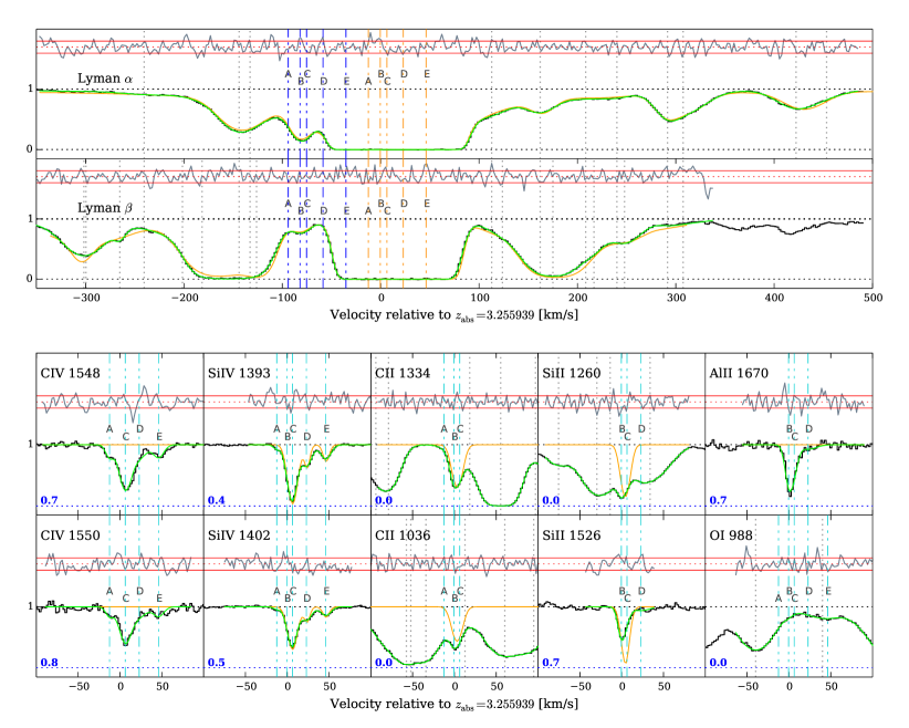
The spectra described in Sec. 2 are kept as independent spectra, rather than combined into one composite spectrum, and the whole set are fitted simultaneously. In total we have 10 metal regions in the system (C iv 1548, C iv 1550, Si iv 1393, Si iv 1402, C ii 1334, C ii 1036, Si ii 1260, Si ii 1526, Al ii 1670, and a Mg ii 2803 blend at ) and two Lyman regions available (Lyman and ). For visualisation we use a weighed stacked spectrum as shown in Fig. 1. Since we only have coverage of the first two Lyman series lines in this absorption system, the hydrogen parameter and column density are not independently well-determined. We explore the consequences of this in Sec. 3.3.1, 3.3.2, 3.3.3.
For all species we vary the summed column densities rather than the individual column densities so as to derive a more accurate estimate of the total column density across the absorption complex. This is achieved by assigning one of the column density parameters to be the column density summed over all components, leaving column density parameters assigned to the remaining individual values. This procedure is beneficial in these circumstances because the summed column density may be well-constrained, whereas the column densities for individual velocity components may not be. We require the ratio of (D i)/(H i) to be identical in all subsystems (velocity components). This equates to assuming the same degree of astration for all components. The overall metalicity of this system is sufficiently low for this to be a reasonable assumption (Sec. 3.5). To check for systematic deviations between the telescopes, we fit each model to the Keck spectra alone, the VLT spectra alone, and to the entire data set including the LRIS data as well.
3.2.1 Continuum and velocity shifts
The spectra are normalised to the quasar emission continuum as part of the initial data processing. There it is assumed that the continuum shape does not change abruptly over small ranges but only varies over long ranges. To allow for any possible local variations, we add a flat continuum to the Voigt profile model around all Lyman lines (and some of the metal lines) to account for any uncertainty in the initial continuum modelling. If the continua slopes are treated as free parameters, the preferred fit values are consistent with zero slope and the the improvement in per degree of freedom () is less than 0.01.
We also allow for a velocity shift between the observations to account for any calibration or slit-centering offsets. The shifts are required to be identical for all regions from the same telescope exposure. The only exception is one of the Si iv regions observed with Keck. The preferred velocity shift differed to the other regions in the same exposure so we introduced that additional free parameter in the fit. We checked that the did not improve by allowing any of the other regions to shift independently. The best fit velocity shifts (given in Table 51) are applied before all spectra are combined for visualisation in Fig. 1.
3.3 Models
The composite spectrum in Fig. 1 clearly shows an absorption line with an off-set of from the centre of the main hydrogen component in both Lyman and . This fits well with the expected off-set of and the lines are clearly narrower than the nearby hydrogen lines and wider than expected for thermally broadened metal lines. These facts strongly suggest that the feature is indeed from D i. It is apparent from the spectrum that Si iv has at least three velocity components, whereas Si ii has a slightly different structure not entirely aligned with that of Si iv. This is not unexpected as Si ii and Si iv have very different ionisation potentials (see Table 2) and are known not always to trace the velocity structure of the lower ionisation species (Wolfe & Prochaska, 2000; Fox et al., 2007). Consequently we group species according to their ionisation potentials and tie line fitting parameters accordingly. We then expect to find the same redshift components in C iv and Si iv, which may not correspond to those seen in C ii, Si ii, and Al ii. All components are linked to a H i component with corresponding D i.
| Element | Atomic mass | |||
|---|---|---|---|---|
| H | 1.01 | 13.60 | — | — |
| D | 2.01 | 14.51 | — | — |
| O | 16.00 | 13.62 | 35.12 | 54.94 |
| C | 12.01 | 11.27 | 24.39 | 64.50 |
| Al | 26.98 | 6.00 | 18.83 | 119.99 |
| Si | 28.09 | 8.16 | 16.34 | 45.14 |
The atomic masses are in units of . is the ionisation energy for the th ionisation level in units of .
The Si iv–C iv complex is best fitted by five components (A, C, D, E, F in Fig. 1), for which the column density of C iv(B) is too low to affect the fit (). An automated model-building software based on genetic algorithms preferred six components, when fitted to Si iv-C iv alone, but the additional component was lost when tying it to H i.
The C ii–Si ii–Al ii complex is fitted by two of the Si iv–C iv components (B, C) as well as one additional component for C ii (A) and one for Si ii–Al ii (D) both sharing redshifts with the Si iv–C iv complex. O i is blended with forest absorption, but we add it to the model tied to the low ionisation group in order to constrain the metallicity (see Sec. 3.5).
3.3.1 Temperature fitting
Most of the components have multiple metals allowing us to fit simultaneously for both temperature and -parameters (see Eqn. 2). This was done for the lower ionisation group, C ii, Si ii, Al ii, H i, D i. The degeneracy between the two parameters depends on the number of available species and their mass differences. By simultaneously solving for temperature we ensure the resulting D i/H i estimate and its error estimate correctly reflect this additional uncertainty in the model. The fitted temperature values and associated error estimates are presented in Table 51.
The ionisation potentials of Si iv and C iv are very different from those of C ii, Si ii, Al ii, H i, D i, and consequently the temperatures for the two groups of gasses should be allowed to vary independently. However, the mass difference between Si iv and C iv is too small to recover both temperature and the turbulent -parameter without additional information, so their -parameters were kept tied. To decide whether the tying should be thermal or turbulent we fitted the entire model with the -parameters un-tied (one fit for each of the components) and compared the preferred values to the ones expected for pure thermal or turbulent broadening. Component A, C, and D were clearly closer to thermal, while E was closer to turbulent. There were no significant differences in the between the models with free parameters and the ones with thermal and turbulent ties, but the tying reduces the number of free parameters and consequently the uncertainty of the D i/H i ratio. However, the stronger physical assumptions about the gas structure may lead to increased systematic uncertainty. Component E was tied turbulently between Si iv, C iv, H i and D i based on a similar reasoning.
3.3.2 Tying everything turbulently
Based on comparison, King et al. (2012) found that approximately 70 per cent of all absorption systems are better fitted by a model with turbulently tied -parameters than one with thermal ties. We examined the -parameters from the baseline model and performed a fit with the -parameters of all subsystems tied turbulently within the ionisation groups. The fit is slightly worse than for temperature fitting (3.3.1) with instead of , but the resulting D i/H i ratio of is completely consistent with the result of the temperature fit of . The reduced number of free parameters leads to very small uncertainties on D i/H i, but at the price of strong assumptions about the gas. Although the majority of systems can be approximated by a turbulent fit, the line broadening is a combined effect of thermal and turbulent broadening and when possible one should fit for both.
3.3.3 All untied
To check that the imposed assumptions on the -parameters are reasonable, we also fitted the baseline model with all -parameters and temperatures untied, allowing each component to have different broadening for each species regardless of which ionisation group it belongs to. However all redshift components were kept tied as for the other models listed, which implies inconsistent physical assumptions - untying b-parameters infers the different species are no longer considered co-spatial, yet keeping redshifts tied maintains the co-spatial assumption. Nonetheless, by obliging VPFIT to maintain the same velocity structure, we get a useful indication of how the final uncertainty estimate on D i/H i in the preferred model benefit from tying the b-parameters in a physically plausible way.
The untying of the -parameters results in a slight decrease of (from 1.13 to 1.12 for 5562 and 5756 degrees of freedom respectively) and a doubling of the D i/H i uncertainty, but with the central values consistent ( and ). The small change in indicates that the baseline model describes the data well, and that little is gained by introducing the extra degrees of freedom by relaxing the physical assumptions of tied temperatures and turbulent flow.
3.3.4 No Si iv and C iv
Due to the large difference in ionisation potential between Si iv-C ivand the lower ions, the Si iv-C iv absorbers do not necessarily contain significant amounts of H i. To check the effect of this assumption we have fitted the base model (3.3.1) excluding the Si iv-C iv regions (varying the continuum normalisations and slopes over Lyman and freely). This results in D i/H i of with a = for degrees of freedom consistent with the base model result.
3.4 Deuterium and hydrogen results
The deuterium and hydrogen column densities and their ratios from the various models are presented in Table 3 with the main result being a D i/H i ratio of from the temperature fit (Sec. 3.3.1). We consider the temperature fit as providing the most realistic parameter error estimates. As Table 3 illustrates, the turbulent model yields a D i/H i error estimate three times smaller, but this error is implausibly small and may be a consequence of the broadening assumptions made and the artificially reduced number of free parameters.
We interpret the consistency across the models as an indication of robust modelling of the absorption system in the sense that relaxing the various assumptions does not alter the final result by more than , but affects the uncertainties as it allows for more freedom in the models. Similarly there is agreement between the analyses of the spectra from the two different telescopes to within .
The quoted uncertainties are purely statistical, but the agreement between the different models and the different data sets suggest a robust measurement.
| Model | Spectra | (D i)) | (H i)) | D i/H i [] | ||
|---|---|---|---|---|---|---|
| Temperature fit (3.3.1) | All | 1.13 | ||||
| Temperature fit (3.3.1) | Keck+LRIS | 1.13 | ||||
| Temperature fit (3.3.1) | VLT+LRIS | 1.02 | ||||
| Turbulent ties (3.3.2) | All | 1.16 | ||||
| All untied (3.3.3) | All | 1.12 | ||||
| No Si iv-C iv (3.3.4) | All | 1.09 |
We have kept three significant figures on the logarithmic parameter errors here merely to illustrate the origin of the final error on our (non-logarithmic) D i/H i ratios in the last column.
3.5 Metallicity
Fields et al. (2001) have explored several chemical evolution models, the simplest of which suggests that for gas with metallicities below 0.1 solar, very little deuterium depletion could have occurred and hence such probes are likely to yield a primordial D i/H i measurement. The same is not true for bimodal star formation models.
The Voigt profile modelling of the observational data yields measurements of the H i, O i, C ii, Al ii, Si ii, C iv and Si iv column densities in individual velocity components across the absorption system. The best-fit parameter results are given in Table 51 (in Appendix A).
We assumed the gas to be in photoionisation equilibrium with the ambient ultraviolet background and used Cloudy (Ferland et al., 2013) to generate gas cloud models whose parameters span an appropriate range for this absorption system. We selected a Haardt-Madau HM05 ultraviolet background999See Section 6.11.8 in http://www.nublado.org/browser/branches/c13_branch/docs/hazy1_c13.pdf to calculate Cloudy models with plane-parallel geometry. Since neither the neutral hydrogen volume density, , nor metallicity, , are known a priori, the initial parameter ranges are kept broad and we computed models in a coarse grid across the particle density range .
O i/H i and Si ii/H i are relatively insensitive to , so a comparison between Cloudymodels and the observed values immediately provides a constraint of approximately . Over this metallicity range, Cloudy models indicate very little sensitivity of the predicted Al ii/Si ii column density ratio to , but strong sensitivity to . Another important ratio is O i/Si ii since these two species are the least susceptible to depletion effects given our system properties. Comparing Cloudy and observed O i/Si ii, we derive an upper limit on the particle density. The lower limit was computed by considering the O i/C ii ratio which gives a conservative range on the allowed range. Fig. 2 shows the determined ranges using several pairs of species. As can be seen, the ionisation pairs agree quite well with one another which leads to the resulting particle density constraint .
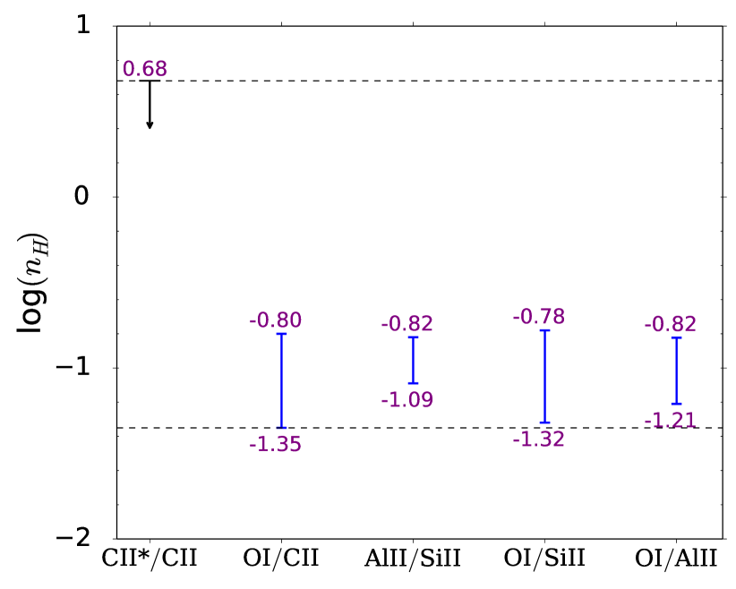
We can compare the range in derived using Cloudy models with that derived using the C ii*/C ii ratio, following the method of detailed balancing using Eqn. 61 in Bahcall & Wolfe (1968). We have ignored the proton collision rate since this should be negligible at the prevailing gas temperature. The electron and hydrogen collision rates were obtained using Eqn. 2 in Blum & Pradhan (1992) and interpolating the values in Tab. 2 of Keenan et al. (1986) respectively. C ii* is not detected in the system but its absence was used to derive an upper limit on the column density. We imposed parameter constraints by assuming the redshifts and -parameters of C ii and corresponding putative C ii* absorption components to be the same. We required N(C ii*) to scale by a common factor to N(C ii) over all corresponding velocity components i. e. N(C ii*) = f N(C ii). VPFIT was then used in an iterative procedure to compute a series of models, for , increasing the value of until the best-fit increased by unity (for , given only one parameter being varied). This procedure yielded independent constraints, and , where is the electron density, which are both consistent with, but considerably less precise than the values derived from the Cloudy models.
Our constraint of may be compared with hydrodynamical simulations of the Lyman- forest; Davé et al. (1998) provide a volume density–column density relation which would suggest a particle density around in our case, inconsistent with our observations. The higher ionisation species C iv and Si iv tend to favour a lower particle density environment and this discrepancy could be resolved by considering single component Cloudy models where these species were detected.
A further consistency check can be derived by comparing the gas temperature returned by the Cloudy models with the temperature estimated during the VPFITing process by solving simultaneously for the turbulent component of the given b-parameter and temperature, using several species. The temperature is estimated as a free parameter for each velocity component in the absorption system. One of the velocity components (B in Fig. 1) which absorbs in all of H i, C ii, Si ii and Al ii yields a reasonably small error estimate for the gas temperature, K (see Appendix A). The other four components have only poorly determined VPFIT temperatures. The Cloudy models relate to the average properties over all five components and gives a temperature in the range K. The apparent VPFIT/Cloudy temperature difference is thus not unexpected.
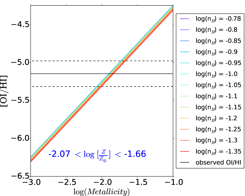
In contrast to Al ii/Si ii, the Cloudy model O i/H i ratio is sensitive to but insensitive to , over the particle density range relevant here. This can be seen from Fig. 3 which indicates an increased sensitivity at lower particle density, however, the constraints developed above enable us to derive a metallicity range of .
4 Discussion
4.1 Line blending
We searched the spectrum for any heavy element absorption systems with commonly found metal lines (Al, Fe, Mg, Si, C) and found tentative systems at 0.56030, 0.56790, 0.60312, 0.89683, 3.00851, 3.09545, 3.25618, 3.29134, 3.45359, 3.55357, 3.57230]. For each of the detected systems we checked whether any metal lines fall in the fitting regions at , i.e. the system we used to measure D i/H i. One blend was identified: Mg ii at falls near H i 1025 in our primary system. To properly account for this we fitted the Mg ii doublet simultaneously in our base model.
4.2 Keck versus VLT
The results from fitting the data from each telescope separately are consistent within albeit the VLT data prefers a lower value of (D i/H i) than the Keck data (D i/H i). Given the difference is well within the statistical uncertainty, the data give us no reason to suspect any kind of systematic explanation, so we ascribe the difference to a random fluctuation.
4.3 Comparison to previous measurements
Crighton et al. (2004) measured the deuterium abundance in the same absorption system to be D i/H i= using a smaller sample of Keck data. This value is below the value obtained here. As shown in Fig. 1 (solid orange) the models appear visually quite similar but there are clear differences. The different D i/H i values are explained by a combination of velocity structure differences and fitting procedures. Compared with Crighton et al. (2004) we increase the observation time by an order of magnitude101010Note we do not include the same data as they used in order to keep the two measurements completely independent. The lower signal-to-noise data revealed fewer velocity components and Crighton et al. (2004) assumed purely thermal broadening between H i and D i, while we have more components and fit for both thermal and turbulent broadening. The re-analysis we present here therefore highlights the importance of high signal-to-noise in deriving a reasonable estimate of the velocity structure in quasar absorption system modelling. The new measurement is closer to the CMB inferred value, but that is not an argument for robustness. Instead the increase in data quality combined with our tests of model assumptions points towards a more robust measurement.
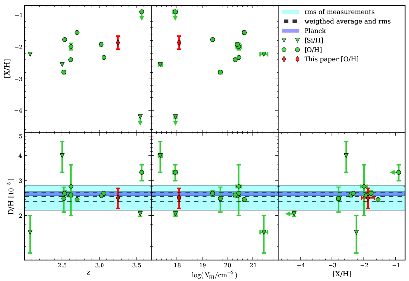
We compare our measurement to the sample from Pettini et al. (2008) plus newer low uncertainty measurements from Fumagalli et al. (2011), Noterdaeme et al. (2012) and Cooke et al. (2014) listed in Table 4. While this is by no means a complete sample, it serves to illustrate the issues and potential of future measurements.
Fig. 4 shows a comparison of the absorption system properties of the measurements given in Table 4. There is no apparent correlation between metallicity, redshift, deuterium or hydrogen column density (rank correlation tests show that the weak anti-correlation between deuterium and column density is not significant).
| Reference | Absorption | H i) | [X/H] | D i/H i | 100 |
| redshift | |||||
| Burles & Tytler (1998a) | 3.572 | <0.9 O | |||
| Burles & Tytler (1998b) | 2.504 | -2.55 Si | |||
| Pettini & Bowen (2001) | 2.076 | -2.23 Si | |||
| Kirkman et al. (2003) | 2.426 | -2.79 O | |||
| Fumagalli et al. (2011) | 3.552 | -4.20 Si | |||
| Noterdaeme et al. (2012) | 2.621 | -1.99 O | |||
| Cooke et al. (2014), Pettini & Cooke (2012) | 3.030 | -1.92 O | |||
| Cooke et al. (2014), O’Meara et al. (2001) | 2.537 | -1.77 O | |||
| Cooke et al. (2014), Pettini et al. (2008) | 2.618 | -2.40 O | |||
| Cooke et al. (2014) | 3.067 | -2.33 O | |||
| Cooke et al. (2014), O’Meara et al. (2006) | 2.702 | -1.55 O | |||
| This work | 3.255 | -1.87 O | |||
| Planck Collaboration et al. (2014)11footnotemark: 1 | — | — | — | — |
Standard flat CDM cosmology for Planck+WP+High
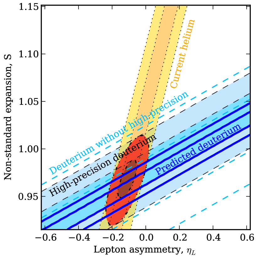
Cooke et al. (2014) presented a new measurement and four re-measurements of the deuterium abundance with very small uncertainties ( per cent) using limiting selection criteria for the absorption systems with , minimum separation of to other absorption systems, at least one unblended optically thin D i transition available, several unblended metal lines with a range of oscillator strength available, high resolution data with resolution and per pixel available) and a “blind” analysis.111111Blind in the sense that no model parameters are viewed until the fitting process has been finalised. This demonstrates the potential of using deuterium as a high-precision probe of cosmological parameters, but the challenge of deciphering the structure of individual systems and the continuum may lead to underestimation of the uncertainties. E.g. the absorption system in Pettini & Cooke (2012, re-analysed in ()) is redshifted so that it falls exactly on top of the Lyman –Nv blend emission from the quasar. To avoid problems like this we need to perform a large number of deuterium measurements and look for a plateau for the primordial value, rather than rely on few values with a possible intrinsic scatter. While the strict criteria of Cooke et al. (2014) do provide high precision measurements, in this paper we have shown that it is possible obtain robust measurements even if we relax the selection criteria and thereby increase the number of usable absorption systems significantly. Fig. 5 shows current and predicted future constraints on non-standard nucleosynthesis from primordial abundances.
4.4 The baryon fraction
D i/H i can be converted to using fitting formulae to Big Bang Nucleosynthesis (BBN) simulations (Simha & Steigman, 2008; Steigman, 2007, 2012)
| (3) |
where is the ratio of the number density of baryons to photons after electron-positron annihilation, the constant depends on the nuclear reaction rates (Steigman, 2012) and the 3 per cent uncertainty reflects the measured uncertainties in the nuclear reaction rates, in particular the D(p,)3He cross section (e.g. Nollett & Holder, 2011). allows for non-standard radiation e.g. such as additional degrees of freedom through the radiation density ,
| (4) |
is the parametrisation of extra radiation in terms of extra neutrino species defined as (see e.g. Riemer-Sørensen et al., 2013). Re-arranging the terms we get
| (5) |
For the standard BBN scenario with the observed values of are given in Table 4.
If D i/H i can be measured to a few percent uncertainty, we will reach a limit where the limiting factor are the nuclear reaction rates. As illustrated in Fig. 5 it will be possible to use D i/H i as a probe of non-standard physics even if this theoretical limit is not improved, if we can beat down the statistical and systematical uncertainty on the observed D i/H i measurements.
5 Conclusions
The presented analysis of high quality spectra from multiple telescopes for the absorption system in J193957-100241 leads to a number of conclusions:
-
•
A D i/H i value of corresponding to = for standard Big Bang nucleosynthesis. The main result was derived with the gas temperature and turbulent broadening as free parameters and fitting for summed column densities. The result is consistent if assuming turbulent broadening only (see Table 3).
-
•
Given the large discrepancy between the previous measurement and the one presented here121212 if naively interpreted as a statistical fluctuation even though it origins in a systematical model difference., we conclude that data quality has a major impact. New and higher quality spectra exist for several of the absorption systems where D i/H i has previously been measured and they should be re-visited.
-
•
We cross check the results between the telescopes and exclude instrument/telescope systematics as a source of scatter in the existing measurements.
-
•
We can obtain high precision measurements from lower column density systems than what is required by Cooke et al. (2014). The spread in column density could be important to understand the scatter among the measurements. Ideally we need a large sample of measurements to identify a plateau of primordial values.
-
•
High-precision measurements of the primordial abundances are a very important cross-check on standard model BBN, and allow us to probe models with non-standard physics. Even though the baryon density can be inferred from high-precision measurements of the CMB, the CMB probes the conditions at the time of recombination (approximately 300,000 years after Big Bang), whereas the primordial abundances probe the epoch of BBN (few minutes) directly. Beyond-standard model physics (e.g. dark matter, extra relativistic particle species etc.) allows for different conditions between the two epochs Steigman (2013), and consequently it is very important to observe both epochs independently.
Acknowledgments
This research is based on observations collected at the European Organisation for Astronomical Research in the Southern Hemisphere, Chile, proposal ID 077.A-0166 obtained by PIs Carswell, Kim, Haehnelt and Zaroubi. It is also based on observations collected with the Keck Observatory Archive (KOA), which is operated by the W. M. Keck Observatory and the NASA Exoplanet Science Institute (NExScI), under contract with the National Aeronautics and Space Administration. The Keck data was obtained by PIs Songaila, Cowie, Crighton and Tytler. We are most grateful to an anonymous referee for a timely and considerate report. MTM thanks the Australian Research Council for Discovery Project grant DP130100568 which supported this work. Parts of this research were conducted by the Australian Research Council Centre of Excellence for All-sky Astrophysics (CAASTRO), through project number CE110001020.
References
- Archidiacono et al. (2014) Archidiacono M., Hannestad S., Sloth Hansen R., Tram T., 2014, ArXiv:1404.5915
- Bagdonaite et al. (2014) Bagdonaite J., Ubachs W., Murphy M. T., Whitmore J. B., 2014, Astrophysical Journal, 782, 10
- Bahcall & Wolfe (1968) Bahcall J., Wolfe R., 1968, Astrophysical Journal, 152
- Battye & Moss (2014) Battye R. A., Moss A., 2014, Physical Review Letters, 112, 051303
- Beringer et al. (2012) Beringer J., et al., 2012, Phys.Rev., D86, 010001
- Blum & Pradhan (1992) Blum R. D., Pradhan A. K., 1992, Astrophysical Journal Supplement, 80, 425
- Bœhm et al. (2013) Bœhm C., Dolan M. J., McCabe C., 2013, Journal of Cosmology and Astroparticle Physics, 8, 41
- Burles et al. (1999) Burles S., Nollett K. M., Truran J. W., Turner M. S., 1999, Physical Review Letters, 82, 4176
- Burles & Tytler (1998a) Burles S., Tytler D., 1998a, Astrophysical Journal, 499, 699
- Burles & Tytler (1998b) Burles S., Tytler D., 1998b, Astrophysical Journal, 507, 732
- Carswell et al. (1984) Carswell R. F., Morton D. C., Smith M. G., Stockton A. N., Turnshek D. A., Weymann R. J., 1984, Astrophysical Journal, 278, 486
- Coc et al. (2014) Coc A., Uzan J.-P., Vangioni E., 2014, Journal of Cosmology and Astroparticle Physics, 10, 50
- Cooke et al. (2014) Cooke R. J., Pettini M., Jorgenson R. A., Murphy M. T., Steidel C. C., 2014, Astrophysical Journal, 781, 31
- Crighton et al. (2004) Crighton N. H. M., Webb J. K., Ortiz-Gil A., Fernández-Soto A., 2004, Monthly Notices of the Royal Astronomical Society, 355, 1042
- Davé et al. (1998) Davé R., Hellsten U., Hernquist L., Katz N., Weinberg D. H., 1998, Astrophysical Journal, 509, 661
- Di Valentino et al. (2013) Di Valentino E., Melchiorri A., Mena O., 2013, Journal of Cosmology and Astroparticle Physics, 11, 18
- Ferland et al. (2013) Ferland G. J., Porter R. L., van Hoof P. A. M., Williams R. J. R., Abel N. P., Lykins M. L., Shaw G., Henney W. J., Stancil P. C., 2013, Revista Mexicana de Astronomía y Astrofísica, 49, 137
- Fields et al. (2001) Fields B. D., Olive K. A., Silk J., Cassé M., Vangioni-Flam E., 2001, Astrophysical Journal, 563, 653
- Fixsen (2009) Fixsen D. J., 2009, Astrophysical Journal, 707, 916
- Forero et al. (2012) Forero D. V., Tórtola M., Valle J. W. F., 2012, Phys. Rev. D, 86, 073012
- Fox et al. (2007) Fox A. J., Ledoux C., Petitjean P., Srianand R., 2007, Astronomy and Astrophysics, 473, 791
- Fukuda et al. (1998) Fukuda Y., Hayakawa T., Ichihara E., et al., 1998, Physical Review Letters, 81, 1562
- Fumagalli et al. (2011) Fumagalli M., O’Meara J. M., Prochaska J. X., 2011, Science, 334, 1245
- Hjerting (1938) Hjerting F., 1938, Astrophysical Journal, 88, 508
- Izotov et al. (2013) Izotov Y. I., Stasińska G., Guseva N. G., 2013, Astronomy and Astrophysics, 558, A57
- Keenan et al. (1986) Keenan F. P., Lennon D. J., Johnson C. T., Kingston A. E., 1986, Monthly Notices of the Royal Astronomical Society, 220, 571
- King et al. (2012) King J. A., Webb J. K., Murphy M. T., Flambaum V. V., Carswell R. F., Bainbridge M. B., Wilczynska M. R., Koch F. E., 2012, Monthly Notices of the Royal Astronomical Society, 422, 3370
- Kirkman et al. (2003) Kirkman D., Tytler D., Suzuki N., O’Meara J. M., Lubin D., 2003, Astrophysical Journal Supplement, 149, 1
- Lanzetta et al. (1991) Lanzetta K. M., Wolfe A. M., Turnshek D. A., Lu L., McMahon R. G., Hazard C., 1991, Astrophysical Journal Supplement, 77, 1
- Nollett & Holder (2011) Nollett K. M., Holder G. P., 2011, ArXiv:1112.2683
- Nollett & Steigman (2014) Nollett K. M., Steigman G., 2014, Phys. Rev. D, 89, 083508
- Noterdaeme et al. (2012) Noterdaeme P., López S., Dumont V., Ledoux C., Molaro P., Petitjean P., 2012, Astronomy and Astrophysics, 542, L33
- O’Meara et al. (2006) O’Meara J. M., Burles S., Prochaska J. X., Prochter G. E., Bernstein R. A., Burgess K. M., 2006, Astrophysical Journal Letters, 649, L61
- O’Meara et al. (2001) O’Meara J. M., Tytler D., Kirkman D., Suzuki N., Prochaska J. X., Lubin D., Wolfe A. M., 2001, Astrophysical Journal, 552, 718
- Pettini & Bowen (2001) Pettini M., Bowen D. V., 2001, Astrophysical Journal, 560, 41
- Pettini & Cooke (2012) Pettini M., Cooke R., 2012, Monthly Notices of the Royal Astronomical Society, 425, 2477
- Pettini et al. (2008) Pettini M., Zych B. J., Murphy M. T., Lewis A., Steidel C. C., 2008, Monthly Notices of the Royal Astronomical Society, 391, 1499
- Planck Collaboration et al. (2014) Planck Collaboration Ade P. A. R., Aghanim N., Armitage-Caplan C., Arnaud M., Ashdown M., Atrio-Barandela F., Aumont J., Baccigalupi C., Banday A. J., et al. 2014, Astronomy and Astrophysics, 571, A16
- Riemer-Sørensen et al. (2013) Riemer-Sørensen S., Parkinson D., Davis T. M., 2013, PASA, 30, 29
- Riemer-Sørensen et al. (2013) Riemer-Sørensen S., Parkinson D., Davis T. M., Blake C., 2013, Astrophysical Journal, 763, 89
- Simha & Steigman (2008) Simha V., Steigman G., 2008, Journal of Cosmology and Astroparticle Physics, 6, 16
- Songaila et al. (1997) Songaila A., Wampler E. J., Cowie L. L., 1997, Nature, 385, 137
- Steigman (2007) Steigman G., 2007, Annual Review of Nuclear and Particle Science, 57, 463
- Steigman (2012) Steigman G., 2012, Advances in High Energy Physics, 268321
- Steigman (2013) Steigman G., 2013, Phys. Rev. D, 87, 103517
- Wolfe & Prochaska (2000) Wolfe A. M., Prochaska J. X., 2000, Astrophysical Journal, 545, 591
- Wyman et al. (2014) Wyman M., Rudd D. H., Vanderveld R. A., Hu W., 2014, Physical Review Letters, 112, 051302
Appendix A Model
| Component | Redshift | Specie | or | [] | |
|---|---|---|---|---|---|
| A | Si iv | 11footnotemark: 1 | — | ||
| C iv | 11footnotemark: 1 | — | |||
| C ii | |||||
| O i | 33footnotemark: 3 | ||||
| H i | |||||
| D i | 33footnotemark: 3 | ||||
| B | Si iv | — | |||
| C ii | |||||
| Si ii | |||||
| Al ii | |||||
| O i | 33footnotemark: 3 | ||||
| H i | |||||
| D i | 33footnotemark: 3 | ||||
| C | Si iv | 11footnotemark: 1 | — | ||
| C iv | 11footnotemark: 1 | — | |||
| C ii | |||||
| Si ii | |||||
| Al ii | |||||
| O i | 33footnotemark: 3 | ||||
| H i | |||||
| D i | 33footnotemark: 3 | ||||
| D | Si iv | 11footnotemark: 1 | — | ||
| C iv | 11footnotemark: 1 | — | |||
| Si ii | |||||
| Al ii | |||||
| O i | 33footnotemark: 3 | ||||
| H i | |||||
| D i | 33footnotemark: 3 | ||||
| E | Si iv | 22footnotemark: 2 | — | ||
| C iv | 22footnotemark: 2 | — | |||
| O i | 33footnotemark: 3 | 22footnotemark: 2 | — | ||
| H i | 22footnotemark: 2 | — | |||
| D i | 33footnotemark: 3 | 22footnotemark: 2 | — | ||
| Summed | Specie | ||||
| Si iv | |||||
| C iv | |||||
| Si ii | |||||
| C ii | |||||
| Al ii | |||||
| O i | |||||
| H i | |||||
| D i |
Thermally tied between C iv and Si iv
22footnotemark: 2Turbulently tied between C iv, Si iv, H i and D i
33footnotemark: 3Ratio tied to H i
The model Blends Redshift Specie b [] C ii 1334 Å 2.62638 H i 13.000 25.07 — 2.62748 H i 14.053 40.42 — 2.62741 H i 13.189 11.71 — 2.62770 H i 13.029 11.32 — 2.62826 H i 12.524 13.40 — 2.62884 H i 13.804 28.45 — 2.62926 H i 13.368 19.32 — 2.63050 H i 14.376 24.45 — C ii 1036 Å 3.67060 H i 12.884 10.31 — 3.67084 H i 13.442 15.46 — 3.67293 H i 14.243 18.73 — 3.67235 H i 13.064 22.47 — 3.67357 H i 12.509 18.84 — 3.67447 H i 14.058 35.56 — 3.67437 H i 13.375 20.72 — 3.67511 H i 13.672 18.31 — Si ii 1526 Å 3.41150 H i 13.062 21.61 — 3.41217 H i 13.586 21.48 — 3.41241 H i 13.290 25.04 — 3.41311 H i 13.499 27.81 — H i 1216 Å 2.59729 H i 12.176 5.67 — 2.59712 H i 12.751 8.83 — 0.56019 Mg ii 11.837 13.73 — 0.56030 Mg ii 13.620 22.00 — 2.59902 H i 12.692 25.43 — 2.58590 H i 12.500 20.27 — 2.58638 H i 12.257 10.18 — 2.58736 H i 13.186 58.58 — 2.58734 H i 13.388 24.43 — 2.58777 H i 12.338 6.03 — 2.58854 H i 13.210 35.19 — 2.58878 H i 13.649 18.10 — 2.58944 H i 13.695 18.54 — 2.59243 H i 12.710 20.65 — 2.59305 H i 14.076 30.07 — 2.59355 H i 12.860 13.58 — 2.59392 H i 13.155 21.44 — H i 1026 Å 3.25253 H i 12.196 29.99 — 3.25405 H i 13.446 47.00 — 3.25390 H i 13.287 21.34 — 3.25754 H i 12.865 23.12 — 3.25824 H i 12.938 19.37 — 3.25889 H i 12.613 34.09 — 3.25935 H i 12.154 17.39 — 3.26008 H i 12.824 14.57 — 3.26030 H i 13.255 28.76 — 3.26193 H i 13.079 25.18 — 3.26238 H i 12.459 22.93 — 3.26368 H i 12.404 5.83 — Velocity shift Data Shift [] setup 2 — setup 5 setup 10 Si iv setup 10 VLT