Study of motion around a static black hole in Einstein and Lovelock gravity

Abstract

We study motion around a static Einstein and pure Lovelock black hole in higher dimensions. It is known that in higher dimensions, bound orbits exist only for pure Lovelock black hole in all even dimensions, $D=2N+2$, where $N$ is degree of Lovelock polynomial action. In particular, we compute periastron shift and light bending and the latter is given by one of transverse spatial components of Riemann curvature tensor. We also consider pseudo-Newtonian potentials and Kruskal coordinates.

I Introduction

Recently Dadhich et al. dadhich showed that pure Lovelock (the equation of motion has only one term corresponding to a fixed $N$) gravity exhibits bound orbits and marginally stable circular orbits around a static black hole in all even $D=2N+2\geq 4$ dimensions, where $N$ is degree of Lovelock polynomial action. This is in contrast to Einstein gravity where bound orbits exist only in $4$ dimensions. Lovelock is the most natural generalization of Einstein gravity and its most remarkable unique property is that inspite of action being polynomial in Riemann curvature, it yields second order equation. It includes Einstein gravity in the linear order $N=1$, Gauss-Bonnet (GB) gravity in the quadratic order $N=2$ and so on.

It would therefore be of interest to study particle and photon orbits around a static Einstein and pure Lovelock (henceforth Lovelock will stand for pure Lovelock) black hole. That is what would be our concern in this paper. For existence of bound orbits what is required is balance between gravitational and centrifugal potentials. The former becomes stronger with dimension for Einstein gravity as it falls off as $1/r^{D-3}$, while the latter always falls off as $1/r^{2}$. Thus for existence of bound orbit what is required is $2>D-3$ and hence no bound orbit exists for $D>4$. On the other hand, Lovelock potential falls off as $1/r^{1/N}$ for even dimensions $D=2N+2$, and since $1/N<2$ for $N\geq 1$, bound orbits will always exist in all even dimensions. Lovelock gravity also exhibits another remarkable property that it is like Einstein in $3$ dimension, kinematic dadhich1 relative to $N$th order Riemann and Ricci curvatures dadhich2 ; dadhich3 . In all odd $D=2N+1$ dimensions gravity is kinematic and there exist analogues of BTZ black holes btz in all odd dimensions. Lovelock gravity is dynamic in even $D=2N+2$ dimensions and that is why bound orbits exist in all even dimensions.

A static spherically symmetric $D$-dimensional metric is defined as

$$ds^{2}=-f(r)dt^{2}+\frac{1}{f(r)}dr^{2}+r^{2}d\Omega_{D-2}^{2},$$ (1)

The effective potential for a test particle moving in such a spherically symmetric space-time is given by

$$V^{2}=f(r)\left(\frac{l^{2}}{r^{2}}+1\right).$$ (2)

For a static black hole in higher dimensional Einstein gravity nuovo we have

$$f(r)=1-\frac{2M}{r^{n}},$$ (3)

while for Lovelock gravity cai

$$f(r)=1-\left(\frac{2M}{r}\right)^{1/N},$$ (4)

where $D=n+3$ and $D=2N+2$, respectively. Here $M$ is an integration constant, which is proportional to the mass ($\mu$) of the black hole and is given by

$$M=\frac{16\pi G\mu}{(D-2)\Omega_{D-2}},$$ (5)

where $G$ is the Newton’s gravitation constant. In particular for $D=4$, $\Omega_{2}=4\pi$ and $M=2G\mu$. Clearly it is the function $f(r)$ that governs motion around the black hole.

In this paper, we wish to explore motion around a static black hole in Lovelock gravity, and compare and contrast it with higher dimensional Einstein gravity. Earlier, geodesic equations in higher dimensional Schwarzschild, Schwarzschild-(anti) de Sitter, Reissner-Nordström and Reissner-Nordström-(anti) de Sitter spacetimes were explored in detail eva . The paper is organized as follows. In the next section we obtain threshold radii for existence, boundedness and stability for circular orbit which is followed by consideration of periastron shift and light bending. In particular light bending turns out to be proportional to one of spatial components of Riemann curvature tensor. Next we obtain the pseudo-Newtonian potential and alternatively obtain the circular orbits threshold radii for boundedness and stability and energy of the marginally stable circular orbit. We also consider Kruskal extension of these black hole metrics and show that only Lovelock metrics accord to the usual form involving exponentials, while for Einstein in higher dimensions there is an additional algebraic factor. We end with a discussion.

II Circular orbits

It is shown in Ref. dadhich that for Einstein gravity bound orbits exist in no other dimension than $4$ while for Lovelock gravity they exist in all even dimensions, $D=2N+2$. We recall the discussion of existence, boundedness and stability of circular orbits in Einstein and Lovelock gravities. The conditions for existence of circular orbits are $\dot{r}=\ddot{r}=0$, bound orbit condition is $E^{2}=1$ and stability is given by the minimum of effective potential, where $r$ and $E$ are the radius of the orbit and specific energy of the test particle, respectively. Photon circular orbit defines the existence threshold.

II.1 Einstein gravity

For the Einstein solution (3), we have

$${E}^{2}=\left(1-\frac{2M}{r^{n}}\right)\left(1+\frac{l^{2}}{r^{2}}\right),$$ (6)

$$\frac{l^{2}}{r^{2}}=\frac{nM}{r^{n}-(n+2)M}.$$ (7)

From these we obtain the existence, stability and boundedness thresholds as

$$r_{ph}=\left((n+2)M\right)^{1/n},$$ (8)

$$r_{s}=\left(\frac{n+2}{2-n}2M\right)^{1/n},$$ (9)

and

$$r_{b}=\left(\frac{4M}{2-n}\right)^{1/n},$$ (10)

respectively. It is clear that bound orbits can exist only for $n=1$ i.e. $D=4$. The energy at the marginally stable circular orbit is given by

$${E_{s}}^{2}=\left(1-\frac{2M}{r_{s}^{n}}\right)\left(1+\frac{l^{2}}{r_{s}^{2}}\right)=\frac{8n}{(n+2)^{2}}.$$ (11)

We get back the Schwarzschild values for $n=1$.

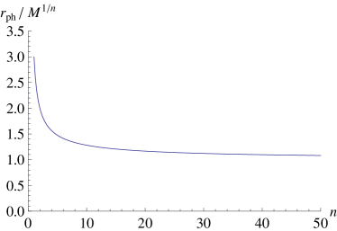
Figure 1: Variation of $r_{ph}$ as a function of $n$ for Einstein gravity.

Figure $1$ shows that the radius of photon orbit gradually decreases with the increase of $n$, because event horizon size also gradually shrinks with increasing $n$.

II.2 Lovelock gravity

The corresponding relations for Lovelock solution (4) are given by

$${E}^{2}=\left(1-\left(\frac{2M}{r}\right)^{1/N}\right)\left(1+\frac{l^{2}}{r^{2}}\right),$$ (12)

$$\frac{l^{2}}{r^{2}}=\frac{(2M)^{1/N}}{r^{1/N}-(2M)^{1/N}},$$ (13)

and

$$r_{ph}=\left(\frac{2N+1}{2N}\right)^{N}2M,$$ (14)

$$r_{s}=\left(\frac{2N+1}{2N-1}\right)^{N}2M,$$ (15)

$$r_{b}=2M\left(\frac{2N}{2N-1}\right)^{N}.$$ (16)

Clearly bound orbits and thereby circular orbits can exist for any $N\geq 1$ in all even dimensions, $D=2N+2$. This is a unique property of (pure) Lovelock gravity.

The energy at the marginally stable circular orbit is given by

$${E_{s}}^{2}=\left(1-\left(\frac{2M}{r_{s}}\right)^{1/N}\right)\left(1+\frac{l^{2}}{r_{s}^{2}}\right)=\frac{8N}{(2N+1)^{2}}.$$ (17)

For $N=1$, it is Einstein gravity and we get back all Schwarzschild values.

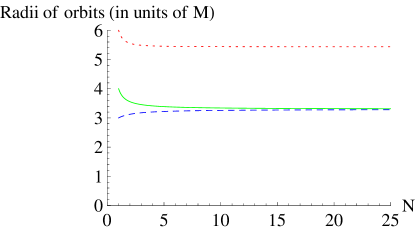
Figure 2: Variations of $r_{ph}$ (dashed line), $r_{b}$ (solid line) and $r_{s}$ (dotted line) as functions of $N$ for pure Lovelock gravity.

Figure $2$ shows that with the increase of $N$, the strength of the potential increases at a given $r$, making $r_{ph}$ merge with $r_{b}$. Increasing strength of gravitational potential decreases $r_{s}$ and $r_{b}$. This is similar to what is observed in Kerr spacetime as compared to Schwarzschild spacetime. Figure $3$ confirms that with increasing $N$, the particle is more bound at $r_{s}$.

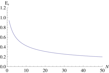
Figure 3: Variation of $E_{s}$ as a function of $N$ for pure Lovelock gravity.

III Light bending and space curvature

It is clear that light cannot feel $\nabla\Phi$ like ordinary massive particles, hence it can only respond to gravity through spacetime curvature. In here we wish to demonstrate that it is infact proportional to transverse component of Riemann curvature. We follow the standard calculations and use the same notations as used in Ref. magnan for the Schwarzschild case.

III.1 Einstein gravity

In spherical symmetry, irrespective of additional angular dimensions, there are two constants of motion. We define them as specific energy $E=\left(1-\frac{2M}{r^{n}}\right)\dot{t}$ and specific angular momentum $l=r^{2}\dot{\phi}$ (which are the same as those for $D=4$ with $\theta=\pi/2$). It then readily follows

$$\left(\frac{1}{r^{2}}\frac{dr}{d\phi}\right)^{2}=\left(\frac{E}{l}\right)^{2}-\left(1-\frac{2M}{r^{n}}\right)\left[\left(\frac{m}{l}\right)^{2}+\frac{1}{r^{2}}\right].$$ (18)

For photon $m=0$ and hence

$$\left(\frac{1}{r^{2}}\frac{dr}{d\phi}\right)^{2}=\left(\frac{E}{l}\right)^{2}-\left(1-\frac{2M}{r^{n}}\right)\frac{1}{r^{2}}.$$ (19)

Let $r=R$, represent the point where photon is closest to the source. Writing $l/E=b$ and at $r=R$, $dr/dt=0$, we have

$$\left(\frac{1}{r^{2}}\frac{dr}{d\phi}\right)^{2}=\left(1-\frac{2M}{R^{n}}\right)\frac{1}{R^{2}}-\left(1-\frac{2M}{r^{n}}\right)\frac{1}{r^{2}}.$$ (20)

We substitute $u=R/r$, such that $u$ lies between $0$ and $1$, and obtain

$$d\phi=\frac{\left(1-u^{2}\right)^{-1/2}du}{\left[1-\frac{2M}{R^{n}}\left(1-u^{n+2}\right)\left(1-u^{2}\right)^{-1}\right]^{1/2}}.$$ (21)

We further put $u=cos\alpha$, where $\alpha$ lies between $0$ and $\pi/2$, and use the approximation for small $M/R$ to obtain

$$\phi=\pi+C_{1}\left(\frac{2M}{R^{n}}\right),$$ (22)

where

$$C_{1}=\int^{\pi/2}_{0}d\alpha[(1-{cos}^{n+2}\alpha){sin}^{-2}\alpha].$$ (23)

Therefore, deflection is given by

$$\Delta\phi=\phi-\pi=C_{1}\left(\frac{2M}{R^{n}}\right).$$ (24)

We find that the value of $C_{1}$ increases with $n$, as given in Table $1$.

III.2 Lovelock gravity

For Lovelock gravity, the metric is given by $(1)$ and $(4)$. Repeating the same calculation, we obtain

$$\phi=\pi+C_{2}\left(\frac{2M}{R}\right)^{1/N},$$ (25)

where,

$$C_{2}=\int^{\pi/2}_{0}d\alpha[(1-{cos}^{2+1/N}\alpha){sin}^{-2}\alpha],$$ (26)

which gives

$$\Delta\phi=C_{2}\left(\frac{2M}{R}\right)^{1/N}.$$ (27)

The value of $C_{2}$ decreases as $N$ increases and it asymptotically converges to $\pi/2$, as given in Table $1$.

III.3 Relation to space curvature

Note that light deflection is proportional to gravitational potential, $M/r^{n}$ and $M/r^{1/N}$ respectively for Einstein and Lovelock black hole. As mentioned before photon can only respond to space curvature, particularly its transverse component, $R^{\theta}{}_{\phi\theta\phi}$, which is the relevant one for deflection and is in fact given by potential and does not involve its derivative. We can thus say that it is space curvature that bends light and its deflection is proportional to transverse space Riemann component.

Table $1$

Variation of $C_{1}$ and $C_{2}$ with spacetime dimension $D$

$D$	$N$	$C_{2}$	$n$	$C_{1}$
4	1	2	1	2
6	2	1.797	3	2.666
10	4	1.687	7	3.657
50	24	1.591	47	8.728
100	49	1.58	97	12.439

IV Bound orbits

As shown in the Introduction, for Einstein gravity bound orbits exist only in $4$ dimensions and none else, while for Lovelock they exist in all even dimensions, $D=2N+2$. We shall consider the two cases of bound orbits corresponding to Lovelock $N=1,2$, that would include usual Schwarzschild case for $N=1$ and $D=4$ and GB case for $N=2$ and $D=6$. We would contrast it with Einstein in $6$ dimensions for $n=3$.

The orbit equation in the usual notation for Einstein in $4$ and $6$ dimensions is given by

$$u^{"}+u=\frac{M}{l^{2}}+3Mu^{2},$$ (28)

$$u^{"}+u=\frac{3Mu^{2}}{l^{2}}+5Mu^{4},$$ (29)

respectively, while for GB it is

$$u^{"}+u=\frac{(2M)^{1/2}u^{-1/2}}{4l^{2}}+\frac{5(2M)^{1/2}u^{3/2}}{4}.$$ (30)

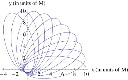
Figure 4: Cartesian plot for Schwarzschild case: $u^{"}+u=1+0.03u^{2}$, where $u=1/r$, using $M=0.01$ and $l=0.1$ and boundary conditions $u(0)=0.1$ and $u^{{}^{\prime}}(0)=0$

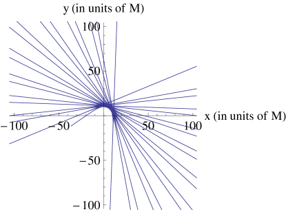
Figure 5: Cartesian plot for Einstein $6D$ case: $u^{"}+u=3u^{2}+0.05u^{4}$, where $u=1/r$, using $M=0.01$ and $l=0.1$ and boundary conditions $u(0)=0.1$ and $u^{{}^{\prime}}(0)=0$

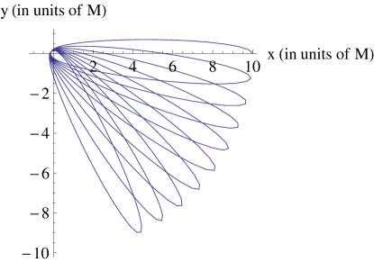
Figure 6: Cartesian plot for Pure Lovelock $6D$ case: $u^{"}+u=3.535u^{-1/2}+0.17675u^{3/2}$, where $u=1/r$, using $M=0.01$ and $l=0.1$ and boundary conditions $u(0)=0.1$ and $u^{{}^{\prime}}(0)=0$

Equation $(28)$ can be solved analytically with some approximations and we obtain a bound orbit which is elliptical in shape with precessing periastron, and it is as given in any textbook, for example, weinberg . However in the other two cases, it is quite difficult to solve the differential equations analytically and we instead solve them numerically.

For Schwarzschild case, we solve $u^{"}+u=1+0.03u^{2}$ by using $M=0.01$ and $l=0.1$. We use the boundary conditions, $u(0)=0.1$ and $u^{{}^{\prime}}(0)=0$. By solving this numerically we obtain elliptical orbits with periastron shifts as expected, shown in Fig. $4$.

For Einstein $6D$ case, $u^{"}+u=3u^{2}+0.05u^{4}$, using $M=0.01$ and $l=0.1$. For boundary conditions $u(0)=0.1$ and $u^{{}^{\prime}}(0)=0$, we see that there does not exist any bound orbit as shown in Fig. $5$. This is consistent with the fact that bound orbits cannot exist in Einstein gravity unless $D=4$ dadhich .

For Lovelock $6D$ case, $u^{"}+u=3.535u^{-1/2}+0.17675u^{3/2}$, using $M=0.01$ and $l=0.1$. For boundary conditions $u(0)=0.1$ and $u^{{}^{\prime}}(0)=0$, we do have bound orbits with precession as exhibited in Fig. $6$. However the orbit is not exactly elliptical and hence shift cannot be called “periastron shift”. Here we have shown that bound orbits exist for $N=2$, similarly they would do so for all $N$ in $D=2N+2$.

V Pseudo-Newtonian potential

The concept of pseudo-Newtonian potential is useful in understanding fluid flow around black holes. Ref. m02 introduces a methodology to evaluate pseudo-Newtonian potential for any metric in general. In the present context, we would like to use it for an alternative computation of circular orbit threshold radii and interestingly it turns out that we obtain the same values as obtained earlier, using general relativity. Note that centrifugal force would go as $1/r^{3}$, while the gradient of pseudo potential would give gravitational force.

Pseudo-Newtonian potential m02 for Einstein and Lovelock cases are given by

$$V=-\frac{M}{r^{n}-2M},$$ (31)

and

$$V=-\frac{(2M)^{1/N}}{2(r^{1/N}-(2M)^{1/N})},$$ (32)

respectively. Then corresponding forces would respectively be given as

$$F=nM\frac{r^{n-1}}{(r^{n}-2M)^{2}},$$ (33)

and

$$F=\frac{(2M)^{1/N}}{2N}\frac{r^{1/N-1}}{(r^{1/N}-(2M)^{1/N})^{2}}.$$ (34)

The Newtonian energy, which is free of rest mass, is defined as

$$\tilde{E}=\frac{v^{2}}{2}+V=\frac{r}{2}\frac{dV}{dr}+V=\frac{r}{2}F+V.$$ (35)

The bound orbit threshold radius would be given by $\tilde{E}=0$, while stability threshold would be given by $dl/dr=0$, and we obtain

$$r_{b}=\left(\frac{4M}{2-n}\right)^{1/n},$$ (36)

and

$$r_{s}=\left(\frac{n+2}{2-n}2M\right)^{1/n},$$ (37)

for the Einstein case, while for Lovelock case,

$$r_{b}=2M\left(\frac{2N}{2N-1}\right)^{N},$$ (38)

and

$$r_{s}=2M\left(\frac{2N+1}{2N-1}\right)^{N}.$$ (39)

These are indeed the same as obtained earlier in Sec II.

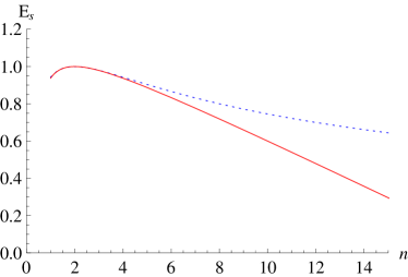
Figure 7: Variation of energy of marginally stable circular orbit for Einstein (dotted line) and pseudo-Newtonian gravity (solid line) with $n$

The energy of marginally stable circular orbit using pseudo-Newtonian potential is given by

$$E_{s}=1+\tilde{E_{s}}=1-\frac{(2N-1)^{2}}{16N}.$$ (40)

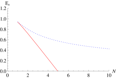
Figure 8: Variation of energy of marginally stable circular orbit for pure Lovelock (dotted line) and pseudo-Newtonian (solid line) gravity with $N$

From Figs. $7$ and $8$, we see that the energy of the marginally stable circular orbit as predicted by the pseudo-Newtonian potential is very close to that of general relativity for the Schwarzschild case i.e. $n=N=1$, but is not so for the higher dimensions. The difference between energies of the last stable circular orbit increases with spacetime dimension for both Einstein and pure Lovelock gravities.

VI Kruskal coordinates

We can carry out Kruskal coordinate transformation for higher dimensional Einstein and Lovelock solutions following the same procedure as that for Schwarzschild metric. We shall perform Kruskal transformation for $D=4,5$ for Einstein and $D=6,8$ for Lovelock black hole.

VI.1 Schwarzschild case ($D=4,n=N=1$)

First we recapitulate the transformation for Schwarzschild metric. We look at null geodesics with $d\theta=d\phi=0$ and use $(3)$ for $n=1$ to obtain

$$dt=\pm\frac{dr}{\left(1-\frac{2M}{r}\right)}.$$ (41)

Integrating $(41)$, we obtain $t=\pm r^{*}+constant$, where $r^{*}$ is the tortoise coordinate given by

$$\small r^{*}=r+2Mlog\left(\frac{r}{2M}-1\right).$$ (42)

The metric then becomes

$$ds^{2}=\left(1-\frac{2M}{r}\right)\left(-dt^{2}+dr^{*2}\right)+r^{2}d\Omega_{2}^{2}.$$ (43)

We further define Eddington-Finkelstein coordinates as $\tilde{u}=t+r^{*}$ and $\tilde{v}=t-r^{*}$. In terms of $\tilde{u}$ and $\tilde{v}$, the metric takes the form

$$ds^{2}=\frac{1}{2}\left(1-\frac{2M}{r}\right)\left(d\tilde{u}d\tilde{v}+d\tilde{v}d\tilde{u}\right)+r^{2}d\Omega_{2}^{2}.$$ (44)

Still $r=2M$ corresponds to either $\tilde{u}=-\infty$ or $\tilde{v}=\infty$, so we further transform coordinates to pull these points to finite coordinate values as

$$u^{{}^{\prime}}=e^{\tilde{u}/4M},\hskip 14.45377ptv^{{}^{\prime}}=e^{-\tilde{v}/4M}.$$ (45)

We thereafter define $u=\frac{1}{2}(u^{{}^{\prime}}-v^{{}^{\prime}})$ and $v=\frac{1}{2}(u^{{}^{\prime}}+v^{{}^{\prime}})$. The metric finally comes to the desired form

$$ds^{2}=\frac{32M^{3}}{r}e^{-r/2M}(du^{2}-dv^{2})+r^{2}d\Omega_{2}^{2}.$$ (46)

The coordinates ($v,u,\theta,\phi$) are the Kruskal coordinates in which metric is regular everywhere except at centre $r=0$, which is the curvature singularity. For constant $r$, $u^{2}-v^{2}=constant$, which is a hyperbola in $u-v$ plane.

VI.2 Einstein gravity ($n=2,3;D=n+3$)

VI.2.1 Einstein 5D $(n=2)$

Using $(3)$ for $n=2$, we write

$$dt=\pm\frac{dr}{\left(1-\frac{2M}{r^{2}}\right)},$$ (47)

which gives $t=\pm r^{*}+constant$, where

$$r^{*}=r+\frac{(2M)^{1/2}}{2}log\left(\frac{r-\sqrt{2M}}{r+\sqrt{2M}}\right)$$ (48)

and the metric reads

$$ds^{2}=\left(1-\frac{2M}{r^{2}}\right)\left(-dt^{2}+dr^{*2}\right)+r^{2}d\Omega_{3}^{2}.$$ (49)

Further to Eddington-Finkelstein coordinates,

$$ds^{2}=\frac{1}{2}\left(1-\frac{2M}{r^{2}}\right)\left(d\tilde{u}d\tilde{v}+d\tilde{v}d\tilde{u}\right)+r^{2}d\Omega_{3}^{2}.$$ (50)

We then transform the coordinates to pull points $\tilde{u}$ and $\tilde{v}$ corresponding to $r=(2M)^{1/2}$ to finite coordinate values as

$$u^{{}^{\prime}}=e^{\tilde{u}/(2M)^{1/2}},\hskip 14.45377ptv^{{}^{\prime}}=e^{-\tilde{v}/(2M)^{1/2}},$$ (51)

and finally we obtain

$$\small ds^{2}=\frac{4M^{2}}{r^{2}}e^{-2r/\sqrt{2M}}\left(\frac{r}{\sqrt{2M}}+1\right)^{2}(-dv^{2}+du^{2})\\ +r^{2}d\Omega_{3}^{2}.$$ (52)

VI.2.2 Einstein 6D $(n=3)$

For $n=3$, we obtain

$$dt=\pm\frac{dr}{\left(1-\frac{2M}{r^{3}}\right)}.$$ (53)

As before, $t=\pm r^{*}+constant$, where

$$\small\begin{split}r^{*}=r+(2M)^{1/3}[\frac{1}{3}log\left(\frac{r}{(2M)^{1/3}}-1\right)\\ -\frac{1}{6}log\left(\frac{r^{2}+(2M)^{1/3}r+(2M)^{2/3}}{(2M)^{2/3}}\right)\\ -\frac{1}{\sqrt{3}}{\tan}^{-1}\left(\frac{2r+(2M)^{1/3}}{\sqrt{3}(2M)^{1/3}}\right)].\end{split}$$ (54)

The forms of the metric in terms of tortoise and Eddington-Finkelstein coordinates are the same as $(49)$ and $(50)$ except for $2M/r^{2}$ replaced by $2M/r^{3}$. We transform the coordinates to pull $\tilde{u}$ and $\tilde{v}$ corresponding to $r=(2M)^{1/3}$ to finite coordinate values as

$$u^{{}^{\prime}}=e^{3\tilde{u}/2(2M)^{1/3}},\hskip 14.45377ptv^{{}^{\prime}}=e^{-3\tilde{v}/2(2M)^{1/3}}.$$ (55)

We then define $u=\frac{1}{2}(u^{{}^{\prime}}-v^{{}^{\prime}})$ and $v=\frac{1}{2}(u^{{}^{\prime}}+v^{{}^{\prime}})$. The metric in terms of $u$ and $v$ is

$$\begin{split}\tiny ds^{2}=\frac{8}{9}\frac{(2M)^{5/3}}{r^{3}}e^{-3r/(2M)^{1/3}}\\ \left(\frac{r^{2}+(2M)^{1/3}r+(2M)^{2/3}}{(2M)^{2/3}}\right)^{3/2}\\ e^{{\sqrt{3}\tan^{-1}(\frac{2r+(2M)^{1/3}}{\sqrt{3}(2M)^{1/3}}})}(du^{2}-dv^{2})+r^{2}d\Omega_{4}^{2}.\end{split}$$ (56)

The coordinate system ($v,u,\theta,\phi$) form the Kruskal coordinate system where $v$ is the time-like coordinate.

VI.3 Lovelock $(N=2,3,D=2N+2)$

We have already considered $N=1$ case for Schwarzschild solution in $D=4$. We would now consider the cases $N=2,3$ and show that proper Kruskal coordinates exist in which metric is free of coordinate singularity.

VI.3.1 Gauss-Bonnet $(N=2,D=6)$

Using $(4)$ for $N=2$, we obtain

$$dt=\pm\frac{dr}{\left(1-(\frac{2M}{r})^{1/2}\right)},$$ (57)

which gives $t=\pm r^{*}+constant$ , where

$$r^{*}=r+(2M)^{1/2}[2\sqrt{r}+2\sqrt{2M}log\left(\frac{\sqrt{r}-\sqrt{2M}}{\sqrt{2M}}\right)].$$ (58)

We follow the same steps as before and first to tortoise coordinates

$$ds^{2}=\left(1-\left(\frac{2M}{r}\right)^{1/2}\right)(-dt^{2}+dr^{*2})+r^{2}d\Omega_{4}^{2},$$ (59)

and then to Eddington-Finkelstein coordinates

$$ds^{2}=\frac{1}{2}\left(1-\left(\frac{2M}{r}\right)^{1/2}\right)\left(d\tilde{u}d\tilde{v}+d\tilde{v}d\tilde{u}\right)+r^{2}d\Omega_{4}^{2}.$$ (60)

Similarly, writing as before

$$u^{{}^{\prime}}=e^{\tilde{u}/8M},\hskip 14.45377ptv^{{}^{\prime}}=e^{-\tilde{v}/8M}.$$ (61)

and defining $u=\frac{1}{2}(u^{{}^{\prime}}-v^{{}^{\prime}})$ and $v=\frac{1}{2}(u^{{}^{\prime}}+v^{{}^{\prime}})$, we obtain the metric in Kruskal coordinates

$$ds^{2}=\frac{32(2M)^{5/2}}{r^{1/2}}e^{-r/4M}e^{-\sqrt{r/2M}}(-dv^{2}+du^{2})+r^{2}d\Omega_{4}^{2}.$$ (62)

VI.3.2 Lovelock $(N=3,D=8)$

Using $(4)$ for $N=3$ gives

$$dt=\pm\frac{dr}{(1-\left(\frac{2M}{r}\right)^{1/3})},$$ (63)

which gives $t=\pm r^{*}+constant$, where

$$\begin{split}r^{*}=r+\frac{3}{2}(2M)^{1/3}r^{2/3}+6Mlog\left(\left(\frac{r}{2M}\right)^{1/3}-1\right)\\ +3(2M)^{2/3}r^{1/3}.\end{split}$$ (64)

The forms of the metric in terms of tortoise and Eddington-Finkelstein coordinates are the same as $(59)$ and $(60)$ except $(2M/r)^{1/2}$ is replaced by $(2M/r)^{1/3}$. We transform the coordinates to pull the points $\tilde{u}$ and $\tilde{v}$ corresponding to $r=2M$ to finite coordinate values as

$$u^{{}^{\prime}}=e^{\tilde{u}/12M},\hskip 14.45377ptv^{{}^{\prime}}=e^{-\tilde{v}/12M}.$$ (65)

The metric in terms of $u$ and $v$ (using the same definition as earlier) is given by

$$\begin{split}ds^{2}=\frac{72(2M)^{7/3}}{r^{1/3}}e^{-r/6M}e^{-\frac{1}{2}(r/2M)^{2/3}}e^{-(r/M)^{1/3}}\\ (-dv^{2}+du^{2})+r^{2}d\Omega_{6}^{2}.\end{split}$$ (66)

As expected, the potential retains its $r^{-k}$ dependence in all the cases. Lovelock case is distinguished from Einstein in that the metric in Kruskal extension always involves exponentials as against additional algebraic factor for Einstein in higher dimensions.

VII Discussion

It is argued in Refs dadhich1 ; dadhich3 that Lovelock gravity has similar behaviour in odd $(2N+1)$ and even $(2N+2)$ dimensions; i.e. similar to Einstein gravity for $N=1$ in $3$ and $4$ dimensions. Here we have employed particle orbits around static black hole and its Kruskal extension to establish this feature. For instance, existence of bound orbits is a universal common feature for Lovelock gravity in all even dimensions. It is also interesting to see that light bending is proportional to transverse spatial Riemann component, $R^{\theta}_{\phi\theta\phi}$. This is to indicate that light does not experience acceleration $\nabla\Phi$, but simply follows the curvature of space. Light bending is in reality space bending which is measured by means of light. For Lovelock black hole, there is always a proper Kruskal extension in all even $D=2N+2$ dimensions in which the metric is free of coordinate singularity similar to $4$-dimensional Schwarzschild solution. In contrast, Einstein metrics in higher dimensions have additional algebraic factor.

Our main aim has been to probe the universal common behaviour of Lovelock gravity by the study of motion around a static black hole, and it has been fully borne out. However one may ask the question, how does the higher dimensional gravitational dynamics affect our observational $4$-dimensional Universe. For instance, in the Kaluza-Klein $5$-dimensional theory, an additional dimension incorporates electromagnetic field. That is, to get higher dimensional effects onto the usual spacetime, some additional prescription has to be imposed like the Kaluza-Klein compactification of extra dimension. For the case of pure Lovelock, the immediate next higher order is quadratic GB, which is topological in $D=4$. It could however be made non-trivial by coupling it with a scalar field — dilaton. There have been extensive studies of dilaton field brax ; cho , however they all refer to Einstein-GB. In line with the viewpoint advocated in this paper and elsewhere dadhich3 ; dadhich1 ; dadhich , it should be pure GB coupled to a scalar field without the Einstein-Hilbert $R$ for probing higher dimensional effects. Very recently, a very interesting and novel inflationary model has been found kgd with a scalar field coupled to pure GB Lagrangian. Another very popular method is brane world gravity randal-sundrum in which curvature of higher dimensional bulk spacetime is employed to make extra dimension small enough. May what all that be, this has not been our concern in this paper.

References

- (1) N. Dadhich, S.G. Ghosh, and S. Jhingan, Phys. Rev. D 88, 124040 (2013).
- (2) N. Dadhich, S.G. Ghosh, and S. Jhingan, Phys. Lett. B 711, 196 (2012).
- (3) N. Dadhich, Pramana 74, 875 (2010).
- (4) N. Dadhich, Gravitational equation in higher dimensions, Proceedings of Relativity and Gravitation: 100 years after Einstein in Prague, June 25-28 (2012).
- (5) M. Bañados, C. Teitelboim, and J. Zanelli, Phys. Rev. Lett. 69, 1849 (1992).
- (6) F.R. Tangherlini, Nuovo Cimento 27, 636 (1963).
- (7) R. Cai and N. Ohta, Phys. Rev. D 74, 064001 (2006); R.-G. Cai, L.-M. Cao, Y.-P. Hu, and S. P. Kim, Phys. Rev. D 78, 124012 (2008); N. Dadhich, Math Today 26, 37 (2011); N. Dadhich, J. M. Pons, and K. Prabhu, Gen. Relativ. Gravit. 45, 1131 (2013).
- (8) E. Hackmann, V. Kagramanova, J. Kunz, and C. Lämmerzahl, Phys. Rev. D 78, 124018 (2008).
- (9) C. Magnan, arXiv:0712.3709v1 [gr-qc].
- (10) S. Weinberg, Gravitation and Cosmology (John Wiley and Sons, New York, 1972).
- (11) B. Mukhopadhyay, Astrophys. J. 581, 427 (2002).
- (12) P. Brax, C. van de Bruck, A.-C. Davis, and D. Shaw, Phys. Rev. D 82, 063519 (2010); P. Kanti, B. Kleihaus, and J. Kunz, Phys. Rev. D 85, 044007 (2012).
- (13) Y.M. Cho, Phys. Rev. Lett. 68, 3133 (1992); T. Damour and K. Nordtvedt, Phys. Rev. D 48, 3436 (1993); T. Damour and K. Nordtvedt, Phys. Rev. Lett. 70, 2217 (1993).
- (14) P. Kanti, R. Gannouji, and N. Dadhich, arXiv:1503.01579v1 [hep-th].
- (15) L. Randall and R. Sundrum, Phys. Rev. Lett. 83, 4690 (1999); L. Randall and R. Sundrum, Phys. Rev. Lett. 83, 3370 (1999).