Einstein-Maxwell gravity coupled to a scalar field in 2+1-dimensions

Abstract

We consider Einstein-Maxwell-self-interacting scalar field theory described by a potential $V\left(\phi\right)$ in $2+1-$dimensions. The self-interaction potential is chosen to be a highly non-linear double-Liouville type. Exact solutions, including chargeless black holes and singularity-free non-black hole solutions are obtained in this model.

I Introduction

Minimally coupled pure scalar field solutions in curved $2+1-$dimensions is severely restricted to admit a variety of solutions 1 . This is in contrast to higher dimensions in which generation of scalar field solutions follow from known vacuum Einstein solutions. The fact that there is no vacuum solution in $2+1-$dimensions makes this method inapplicable. The strategy therefore is followed by adding sources such as cosmological constant 2 ; 3 , electromagnetic (both linear and non-linear) field 4 ; 5 ; 6 and non-minimally coupled scalar fields to couple with such sources 7 ; 8 ; 9 . Self-interacting scalar fields as a potential term in the Lagrangian is also an alternative method to investigate the role / effects of scalar fields 10 ; 11 ; 12 ; 13 ; 14 ; 15 . A well-known class of self-interacting scalar fields for instance is given by global monopole 16 which arises as a result of spontaneous symmetry breaking. The idea is to search for black holes with scalar hairs in analogy with the electromagnetic fields. In this regard scalar fields alone in higher dimensions ($D>3$) creates mostly naked singularities and very rarely black holes. The singular solution by Janis, Newman and Winicour 17 is a prototype in this regard in $3+1-$dimensions. The solution by Bocharova-Bronnikov-Melnikov-Bekenstein (BBMB) provides a black hole solution in the same dimensionality 18 ; 19 . The massive scalar field in three dimensions has been also considered in 20 ; 21 ; 22 .

In this study we consider minimally coupled scalar, Maxwell fields and a self-interaction potential $V\left(\phi\right)$ for the scalar field. Our choice for the potential is in the form of a double-Liouville potential 23 of the form $V\left(\phi\right)=\lambda_{1}e^{\alpha_{1}\phi}+\lambda_{2}e^{\alpha_{2}\phi}$ in which $\lambda_{i}$ and $\alpha_{i}$ are constant parameters. It should be added that this form of potential is not reducible to a single-Liouville potential $V\left(\phi\right)=\lambda e^{\alpha\phi}$ with constant $\lambda$ and $\alpha$. The occurrence of extra parameters doesn’t create redundancy in the problem and as a matter of fact it renders the solution possible. Certain solutions may arise in which some parameters are dispensable. As it will be observed the Liouville-type potential is too strong and creates singularity at the origin. We show that black hole solutions can also be obtained along with the non-black hole solutions in such a model. This happens as a result of tuning our free parameters. With zero electric charge, for instance, the Einstein-Scalar system gives rise to a black hole solution with constant Hawking temperature. More general solutions can be obtained as a result of reduction of the system of equations into a Riccati type. We find as an example chargeless, singularity free solution that at infinity becomes conformal to the BTZ spacetime.

Organization of the paper goes as follows. In Section II we derive the field equations of our model. Exact black hole solutions are represented with zero electric charge in Section III. Non-black hole solutions, both singular and non-singular are given in Section IV. The paper ends with Conclusion in Section V.

II Einstein-Maxwell gravity coupled to a scalar field

The action of Einstein-Maxwell gravity coupled minimally to a scalar field $\phi$ is given by ($16\pi G=c=1$)

$$S=\int d^{3}x\sqrt{-g}\left(\mathcal{R}-2\partial_{\mu}\phi\partial^{\mu}\phi-F^{2}-V\left(\phi\right)\right)$$ (1)

in which $F=F_{\mu\nu}F^{\mu\nu}$ stands for the Maxwell invariant and $V\left(\phi\right)$ is to be chosen (We would like to note that our formalism follows the higher dimensional version of 24 ; 25 ). The Field equations are given by applying the variational principles,

$$d\left({}^{\star}\mathbf{F}\right)=0,$$ (2)

$$\square\phi=\frac{1}{4}\frac{dV}{d\phi},$$ (3)

and

$$G_{\mu}^{\nu}=T_{\mu}^{\nu}$$ (4)

in which

$$T_{\mu}^{\nu}=2\left(F_{\mu\lambda}F^{\nu\lambda}-\frac{1}{4}F_{\alpha\beta}F^{\alpha\beta}\delta_{\mu}^{\nu}\right)+\\ 2\left(\partial_{\mu}\phi\partial^{\nu}\phi-\frac{1}{2}\partial_{\lambda}\phi\partial^{\lambda}\phi\delta_{\mu}^{\nu}\right)-\frac{1}{2}V\left(\phi\right)\delta_{\mu}^{\nu},$$ (5)

and $\square$ stands for the covariant Laplacian. The spacetime under study is static and circularly symmetric with a line element of the form

$$ds^{2}=-U\left(r\right)dt^{2}+\frac{dr^{2}}{U\left(r\right)}+R^{2}\left(r\right)d\theta^{2}$$ (6)

in which $U\left(r\right)$ and $R\left(r\right)$ are the metric functions to be found. The electric field ansatz $2-$form is

$$\mathbf{F}=\frac{q}{R}dt\wedge dr$$ (7)

in which $q$ is the electric charge. Considering this ansatz, we find the following field equations,

$$\left(RU\phi^{\prime}\right)^{\prime}=\frac{R}{4}\frac{dV}{d\phi},$$ (8)

$$\frac{R^{\prime\prime}}{R}=-2\phi^{\prime 2},$$ (9)

$$\left(RU\right)^{\prime\prime}=-3RV-\frac{2q^{2}}{R}$$ (10)

and

$$\left(UR^{\prime}\right)^{\prime}=-\frac{2q^{2}}{R}-RV.$$ (11)

III An exact black hole solution

In this chapter we give an exact solution with the double Liouville potential

$$V\left(\phi\right)=\lambda_{1}e^{\alpha_{1}\phi}+\lambda_{2}e^{\alpha_{2}\phi}$$ (12)

in which $\lambda_{i}$ and $\alpha_{i}$ are some constants. Let us add that the choice of double-potential term can’t be reduced through reparametrization into a single-Liouville potential. The advantage of employing more parameters will be clear subsequently. Our ansatz for $R$ is

$$R=e^{A\phi}$$ (13)

in which $A$ is a constant to be found. Plugging these into the field equations yields the following solution for the scalar field

$$\phi=\frac{A\ln\left(1+\frac{r}{r_{0}}\right)}{A^{2}+2}$$ (14)

in which $r_{0}$ is an integration constant. With $\alpha_{1}=-\frac{4}{A}$ and $\alpha_{2}=-2A$ one also finds

$$U\left(r\right)=C_{1}\left(1+\frac{r}{r_{0}}\right)^{\frac{2}{A^{2}+2}}-\frac{\lambda_{1}r_{0}^{2}\left(A^{2}+2\right)^{2}}{2A^{2}\left(A^{2}-1\right)}\left(1+\frac{r}{r_{0}}\right)^{\frac{2A^{2}}{A^{2}+2}}\\ -\frac{\left(\lambda_{2}+2q^{2}\right)r_{0}^{2}\left(A^{2}+2\right)^{2}}{2A^{2}}\left(1+\frac{r}{r_{0}}\right)^{\frac{4}{A^{2}+2}}$$ (15)

in which $C_{1}$ is another integration constant and the parameter $A$ is given by

$$A^{2}=2\left(1+\frac{2q^{2}}{\lambda_{2}}\right).$$ (16)

We note that the electric charge $q$ and $\lambda_{2}$ must be chosen in such a way that $1+\frac{2q^{2}}{\lambda_{2}}>0$ and $1+\frac{2q^{2}}{\lambda_{2}}\neq\frac{1}{2}.$ This guarantees that $A^{2}\neq 0,1$ and remains positive. The form of the electric field in its closed form reads

$$E=qe^{-A\phi}=q\left(\frac{r_{0}}{r+r_{0}}\right)^{\frac{A^{2}}{A^{2}+2}}.$$ (17)

It should be added that by introducing $\rho=1+\frac{r}{r_{0}}$ and $\tau=r_{0}t$ the line element becomes

$$ds^{2}=-f\left(\rho\right)d\tau^{2}+\frac{d\rho^{2}}{f\left(\rho\right)}+\rho^{\frac{2A^{2}}{A^{2}+2}}d\theta^{2}$$ (18)

in which

$$f\left(\rho\right)=\tilde{C}_{1}\rho^{\frac{2}{A^{2}+2}}-\frac{\lambda_{1}\left(A^{2}+2\right)^{2}}{2A^{2}\left(A^{2}-1\right)}\rho^{\frac{2A^{2}}{A^{2}+2}}-\\ \frac{\left(\lambda_{2}+2q^{2}\right)\left(A^{2}+2\right)^{2}}{2A^{2}}\rho^{\frac{4}{A^{2}+2}}$$ (19)

for $\tilde{C}_{1}=\frac{C_{1}}{r_{0}^{2}}.$ We notice that the case with $A^{2}=2$ yields $q=0,$ $\alpha_{1}=\alpha_{2}=-2\sqrt{2}$ with the metric function

$$f\left(\rho\right)=\tilde{C}_{1}\sqrt{\rho}-4\left(\lambda_{1}+\lambda_{2}\right)\rho$$ (20)

and the line element

$$ds^{2}=-f\left(\rho\right)d\tau^{2}+\frac{d\rho^{2}}{f\left(\rho\right)}+\rho d\theta^{2}.$$ (21)

We set $\rho=x^{2}$ to get

$$ds^{2}=-f\left(x\right)d\tau^{2}+\frac{4x^{2}dx^{2}}{f\left(x\right)}+x^{2}d\theta^{2},$$ (22)

with

$$f\left(x\right)=\tilde{C}_{1}x-4\left(\lambda_{1}+\lambda_{2}\right)x^{2}.$$ (23)

Depending on the sign of $\tilde{C}_{1}$ and $\lambda_{1}+\lambda_{2}$ the corresponding spacetime can be black hole or not. For the case of the black hole we consider $4\left(\lambda_{1}+\lambda_{2}\right)=-\frac{1}{\ell^{2}}$ and $\tilde{C}_{1}=-a$ so that we find

$$f\left(x\right)=\frac{x^{2}}{\ell^{2}}-ax$$ (24)

with an event horizon at $x_{h}=a\ell^{2}$ and line element

$$ds^{2}=-\frac{x}{\ell^{2}}\left(x-x_{h}\right)d\tau^{2}+\frac{4x\ell^{2}dx^{2}}{\left(x-x_{h}\right)}+x^{2}d\theta^{2}.$$ (25)

The Ricci and Kretschmann scalars are found to be singular at $x=0,$ given respectively by

$$\mathcal{R}=-\frac{2x+x_{h}}{4x^{3}\ell^{2}}$$ (26)

and

$$\mathcal{K}=\frac{4x^{2}-4x_{h}x+3x_{h}^{2}}{16x^{6}\ell^{4}}.$$ (27)

The scalar field reads

$$\phi=\frac{\ln x}{\sqrt{2}}$$ (28)

with the potential

$$V\left(\phi\right)=\frac{\lambda_{1}+\lambda_{2}}{x^{2}}.$$ (29)

The corresponding Hawking temperature is found as

$$T_{H}=\left(\frac{-g_{tt}^{\prime}}{4\pi\sqrt{-g_{tt}g_{xx}}}\right)_{x=x_{h}}=\frac{1}{8\pi\ell^{2}},$$ (30)

which is constant. This signals an isothermal Hawking process in analogy with a linear dilaton black hole in $3+1-$dimensions. Using the standard entropy i.e.,

$$S=\pi x_{h}$$ (31)

one finds that the specific heat capacity becomes

$$C_{q}=T_{H}\left(\frac{\partial S}{\partial T_{H}}\right)_{q}=0.$$ (32)

III.1 Exact solution with $A=1.$

As we mentioned before, the case $A=1$ is excluded in the previous section. Here we give the solution separately when $A=1.$ The field equations admit

$$\phi=\frac{\ln r}{3}$$ (33)

and

$$U\left(r\right)=C_{1}r^{2/3}-9q^{2}r^{4/3}-\frac{9\lambda_{2}r^{4/3}}{2}-3\lambda_{1}r^{2/3}\ln r$$ (34)

where $C_{1}$ is an integration constant. The line element may be written as

$$ds^{2}=-U\left(y\right)dt^{2}+\frac{36y^{10}dy^{2}}{U\left(y\right)}+y^{2}d\theta^{2},$$ (35)

in which we set $r^{1/3}=y^{2}$ and

$$U\left(y\right)=y^{4}\left(C_{1}-9\left(q^{2}+\frac{\lambda_{2}}{2}\right)y^{4}-18\lambda_{1}\ln y\right).$$ (36)

We note that the line element (36) can be a black hole or a naked singular spacetime. Its Ricci scalar is given by

$$\mathcal{R}=\frac{-10\lambda_{1}\ln y+11\left(q^{2}+\frac{\lambda_{2}}{2}\right)y^{4}+\frac{5C_{1}}{9}+4\lambda_{1}}{2y^{8}}.$$ (37)

In the case of the black hole with an event horizon at $y=y_{h}\neq 0$ one finds the Hawking temperature

$$T_{H}=-\frac{3\left(\left(2q^{2}+\lambda_{2}\right)y_{h}^{4}+\lambda_{1}\right)}{4\pi y_{h}^{2}}$$ (38)

and heat capacity as

$$C_{q}=\frac{\pi y_{h}\left[y_{h}^{4}\left(2q^{2}+\lambda_{2}\right)+\lambda_{1}\right]}{2\left[y_{h}^{4}\left(2q^{2}+\lambda_{2}\right)-\lambda_{1}\right]}.$$ (39)

A phase change at $y_{h}^{4}\left(2q^{2}+\lambda_{2}\right)-\lambda_{1}=0$ can occur but for the large enough horizon $C_{q}>0$ which indicates the thermodynamical stability of the solution.

IV Construction of the General solution

Next, let us introduce $K=-2\phi^{\prime 2},$ $R=\exp\left(\int Ydr\right)$ and $u=UR$ which transform the field equations into the Riccati form

$$Y^{2}+Y^{\prime}=K,$$ (40)

with

$$u^{\prime\prime}=-3V\exp\left(\int Ydr\right)-2q^{2}\exp\left(-\int Ydr\right),$$ (41)

$$\left(u\phi^{\prime}\right)^{\prime}=\frac{\exp\left(\int Ydr\right)}{4}\frac{dV}{d\phi}$$ (42)

and

$$\left(uY\right)^{\prime}=-2q^{2}\exp\left(-\int Ydr\right)-V\exp\left(\int Ydr\right).$$ (43)

We combine (41) and (43) to eliminate $V$ i.e.,

$$u^{\prime\prime}-3\left(uY\right)^{\prime}=4q^{2}\exp\left(-\int Ydr\right).$$ (44)

An integration implies

$$u^{\prime}-3uY=4q^{2}\int dr\exp\left(-\int Ydr\right)+c_{1}$$ (45)

in which $c_{1}$ is an integration constant. Upon using $Y=\frac{R^{\prime}}{R}$ one finds

$$u=R^{3}\left(\int\frac{1}{R^{3}}\left[4q^{2}\int\frac{dr}{R}+c_{1}\right]dr+c_{2}\right)$$ (46)

in which $c_{2}$ is another integration constant. Having $u$ one finds from (41)

$$V=-\frac{u^{\prime\prime}}{3R}-\frac{2q^{2}}{3R^{2}}.$$ (47)

IV.1 An Explicit Example

To find an explicit solution one has to choose an ansatz for $\phi$ and then by following the results given above, to find the other unknown functions.

IV.1.1 $\phi=\alpha\ln\left(\frac{r}{r_{0}}\right)$

Our choice for $\phi$ is a logarithmic function of the form

$$\phi=\alpha\ln\left(\frac{r}{r_{0}}\right)$$ (48)

in which $\alpha$ and $r_{0}$ are two constants. Upon (48), the Riccati equation becomes

$$Y^{2}+Y^{\prime}=-2\phi^{\prime 2}$$ (49)

with a solution of the form

$$Y=\frac{A}{r}$$ (50)

in which $A$ is a constant, satisfying

$$A^{2}-A+2\alpha^{2}=0.$$ (51)

This condition imposes that $0<A<1.$ Consequently one finds

$$R=\exp\left(\int Ydr\right)=\left(\frac{r}{r_{1}}\right)^{A}$$ (52)

in which $r_{1}$ is an integration constant. Next, we find

$$u=\frac{2q^{2}r_{1}^{2}}{\left(1-A\right)\left(1-2A\right)}\left(\frac{r_{1}}{r}\right)^{A-2}+\\ \frac{c_{1}}{1-3A}r+c_{2}\left(\frac{r}{r_{1}}\right)^{3A}$$ (53)

for $A\neq 1/3,1/2.$ Finally, the potential $V$ is found to be

$$V=\frac{2q^{2}\left(1-A\right)}{3\left(1-2A\right)}\left(\frac{r}{r_{1}}\right)^{-2A}-\\ \frac{c_{2}A\left(3A-1\right)}{r_{1}^{2}}\left(\frac{r}{r_{1}}\right)^{2\left(A-1\right)}.$$ (54)

One can use the inverse transformation to find

$$U=\frac{2q^{2}r_{1}^{2}}{\left(1-A\right)\left(1-2A\right)}R^{\frac{2}{A}-2}+\frac{c_{1}}{1-3A}r_{1}R^{\frac{1}{A}-1}+c_{2}R^{2}$$ (55)

and as a result

$$V\left(\phi\right)=\frac{2q^{2}\left(1-A\right)}{3\left(1-2A\right)}\left(\frac{r_{1}}{r_{0}}\right)^{2A}e^{-2A\phi/\alpha}-\\ \frac{c_{2}A\left(3A-1\right)}{r_{1}^{2}}\left(\frac{r_{1}}{r_{0}}\right)^{2\left(1-A\right)}e^{2\left(1-A\right)\phi/\alpha}.$$ (56)

We note that, $\alpha,$ $A,$ $r_{0},$ $r_{1},$ $c_{1}$ and $c_{2}$ are parameters to be chosen provided the constraint (51) is satisfied. One of the simplest choice of the parameters can be given if we set $q=c_{1}=0$ and $c_{2}=1.$ The line element, hence, becomes

$$ds^{2}=U\left(-dt^{2}+d\theta^{2}\right)+\frac{dr^{2}}{U}$$ (57)

in which $U=\left(\frac{r}{r_{1}}\right)^{2A}.$ The potential, accordingly, reads as

$$V\left(\phi\right)=\frac{A\left(3A-1\right)}{r_{1}^{2}}\left(\frac{r_{1}}{r_{0}}\right)^{2\left(1-A\right)}e^{2\left(1-A\right)\phi/\alpha}$$ (58)

in which $\phi$ is given by (48). It is observed that the case $A=1$ is not included in our solution. The latter case has been found in 7 ; 8 ; 9 . Here in our solution $0<A<1$ and one of the simplest choice of $A$ is $\frac{1}{2}$ which yields $\alpha=\pm\frac{1}{2\sqrt{2}}$, $U=\frac{r}{r_{1}}$ and

$$V\left(\phi\right)=\frac{1}{4r_{0}r_{1}}e^{\pm 2\sqrt{2}\phi}$$ (59)

while $\phi=$ $\pm\frac{1}{2\sqrt{2}}\ln\left(\frac{r}{r_{0}}\right).$ (We note that with $q=c_{1}=0$ the solution for $A=\frac{1}{2}$ (for $q=0$) is the same as (29)). The resulting line element, then, becomes (let’s set $r_{0}=1$)

$$ds^{2}=\left(\frac{r}{r_{1}}\right)\left(-dt^{2}+d\theta^{2}\right)+\left(\frac{r_{1}}{r}\right)dr^{2}.$$ (60)

Schmidt and Singleton found this solution in their work 10 where $U=\left(\frac{r}{\ell}\right)^{2},$ $\phi\sim\ln r$ and $V\left(\phi\right)\sim e^{-2\sqrt{\kappa}\phi}.$

Our new solution which we shall proceed, begins with the case when $c_{1}=0,$ $c_{2}\neq 0$ and $A=\frac{2}{3}.$ The metric function then becomes

$$U=-18q^{2}r_{1}^{2}R+c_{2}R^{2}$$ (61)

for

$$R=\left(\frac{r}{r_{1}}\right)^{\frac{2}{3}}.$$ (62)

This solution is not a black hole since a regular horizon doesn’t exist. The metric function becomes by the choice $c_{2}=18q^{2}r_{1}^{2}$

$$U=\chi r^{\frac{2}{3}}\left(r^{\frac{2}{3}}-r_{1}^{\frac{2}{3}}\right)$$ (63)

in which $\chi=18q^{2}r_{1}^{\frac{2}{3}}.$

IV.2 A bounded regular solution

In this section we set $q=0,$ $\phi=\frac{r}{r_{0}}$ in which for our later convenience we set $r_{0}=\sqrt{2}.$ The Eq. (49) becomes

$$Y^{2}+Y^{\prime}=-1$$ (64)

with the solution given by

$$Y=-\tan r$$ (65)

and consequently

$$R\left(r\right)=\left|\cos r\right|$$ (66)

and

$$u\left(r\right)=\frac{\xi_{1}}{2}\cos r\left(\sin r+\cos^{2}r\ln\left|\sec r+\tan r\right|\right)+\xi_{2}\cos^{3}r.$$ (67)

Finally

$$U\left(r\right)=\frac{\xi_{1}}{2}\left(\sin r+\cos^{2}r\ln\left|\sec r+\tan r\right|\right)+\xi_{2}\cos^{2}r$$ (68)

in which $\xi_{1}$ and $\xi_{2}$ are two integration constants and

$$V\left(r\right)=\xi_{2}\left(-2+3\cos^{2}r\right)+\\ \xi_{1}\left[\frac{3}{2}\sin r+\frac{\left(-2+3\cos^{2}r\right)}{2}\ln\left(\frac{1+\sin r}{\cos r}\right)\right].$$ (69)

With $\xi_{1}=0$ the line element becomes

$$ds^{2}=-\xi_{2}\cos^{2}rdt^{2}+\frac{dr^{2}}{\xi_{2}\cos^{2}r}+\cos^{2}rd\theta^{2}.$$ (70)

Next, we apply the following change of variable

$$x=\cos r$$ (71)

which implies

$$ds^{2}=-\xi_{2}x^{2}dt^{2}+\frac{dx^{2}}{\xi_{2}x^{2}\left(1-x^{2}\right)}+x^{2}d\theta^{2}$$ (72)

with $\left|x\right|<1$ whose scalar curvature and Kretschmann scalar are

$$\mathcal{R}=\xi_{2}\left(10x^{2}-6\right)$$ (73)

and

$$\mathcal{K}=4\xi_{2}^{2}\left(17x^{4}-20x^{2}+6\right).$$ (74)

The potential, becomes

$$V\left(\phi\right)=\xi_{2}\left(-2+3\cos^{2}\left(\sqrt{2}\phi\right)\right)$$ (75)

with the scalar field

$$\phi=\frac{\arccos x}{\sqrt{2}}.$$ (76)

We apply now a new transformation which maps $x\in\left(-1,1\right)$ into $\rho\in\left[0,\infty\right)$ as defined by

$$\rho=\sqrt{\frac{x^{2}}{1-x^{2}}}$$ (77)

with the transformed line element (we note that $\xi_{2}>0$ has no role in the scalars and therefore we set it as $\xi_{2}=1$)

$$ds^{2}=\frac{1}{1+\rho^{2}}\left(-\rho^{2}dt^{2}+\frac{d\rho^{2}}{\rho^{2}}+\rho^{2}d\theta^{2}\right).$$ (78)

Also the scalar field becomes

$$\phi=\frac{\arccos\left(\frac{\rho}{\sqrt{1+\rho^{2}}}\right)}{\sqrt{2}}$$ (79)

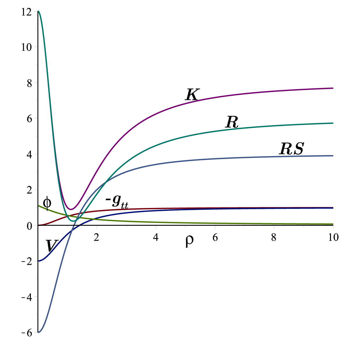
Figure 1: A plot of $V\left(\rho\right),$ $\phi\left(\rho\right),$ $\mathcal{R}$, $\mathcal{RS}$, $\mathcal{K}$ and $-g_{tt}$ with respect to $\rho.$ The astrophysical object is regular everywhere and asymptotically, for $\rho\rightarrow\infty,$ it becomes conformal to the AdS spacetime..

with the potential

$$V\left(\rho\right)=\frac{\rho^{2}-2}{\rho^{2}+1}.$$ (80)

It is observed that the scalars take the forms

$$\mathcal{R}=\frac{2\left(2\rho^{2}-3\right)}{1+\rho^{2}}$$ (81)

$$\mathcal{RS}=R_{\mu\nu}R^{\mu\nu}=\frac{2\left(6-8\rho^{2}+3\rho^{4}\right)}{\left(1+\rho^{2}\right)^{2}}$$

and

$$\mathcal{K}=\frac{4\left(3-4\rho^{2}+2\rho^{4}\right)}{\left(1+\rho^{2}\right)^{2}}.$$ (82)

The spacetime given by (78) is not a black hole and also is not singular. This is a regular object with scalar invariant everywhere in the domain of $\rho\in\left[0,\infty\right).$ In Fig. 1 we plot $V\left(\rho\right)$, $\phi\left(\rho\right)$, $\mathcal{R}$, $\mathcal{RS}$, $\mathcal{K}$ and $-g_{tt}$ in terms of $\rho$ which display the general behavior of the cosmological object in the domain of $\rho.$

V Conclusion

To what extent self-interacting scalar fields play role in lower dimensions such as $2+1$?. Can scalar charge be chosen to imitate the role of electric charge in making of black holes?. These are the problems that we addressed / answered in this paper. We obtained both exact black hole and non-black hole solutions described by potentials of the form $V\left(\phi\right)\sim\lambda_{1}e^{\alpha_{1}\phi}+\lambda_{2}e^{\alpha_{2}\phi}$ with $\lambda_{i}$ and $\alpha_{i}$ constants, coupled to a charged mass / black hole. In particular, we obtain black hole solutions with zero electric charge when the parameters are tuned. The non-black hole solutions give rise to singularities which are strongly naked. The system is described effectively by a Riccati type differential equation. By changing the ansatz for the scalar field our model can be shown to admit different classes of solutions so that the solution space is quite large. As a particular example we present a bounded, completely regular solution which is asymptotically, i.e. for $\rho\rightarrow\infty,$ conformal to the AdS spacetime. This admits a finite potential-well at the origin to attract interest from field theoretical point of view.

References

- (1) K. S. Virbhadra, Pramana 44, 317 (1995).
- (2) M. Bañados, C. Teitelboim, J. Zanelli, Phys. Rev. Lett. 69, 1849 (1992).
- (3) M. Bañados, M. Henneaux, C. Teitelboim and J. Zanelli, Phys. Rev. D 48, 1506 (1993).
- (4) C. Martinez, C. Teitelboim and J. Zanelli, Phys. Rev. D 61, 104013 (2000).
- (5) S. Carlip, Quantum Gravity in 2 + 1 Dimensions, Cambridge University Press, 1998.
- (6) S. Carlip, Living Rev. Rel. 8, 1 (2005).
- (7) E. Ayón-Beato, A. Garcia, A. Macias, J. Perez-Sanchez, Phys. Lett. B 495, 164 (2000).
- (8) E. Ayón-Beato, C. Martínez and Jorge Zanelli, Gen. Rel. Grav. 38, 145 (2006).
- (9) J. Gegenberg, C. Martinez and R. Troncoso, Phys. Rev. D 67, 084007 (2003).
- (10) H-J. Schmidt and D. Singleton, Phys. Lett. B 721, 294 (2013).
- (11) L. Zhao, W. Xu and B. Zhu, Commun. Theor. Phys. 61, 475 (2014).
- (12) W. Xu and L. Zhao, Phys. Rev. D 87, 124008 (2013).
- (13) W. Xu, L. Zhao and D.-C. Zou, arXiv:1406.7153.
- (14) W. Xu and D.-C. Zou, arXiv:1408.1998.
- (15) D.-C. Zou, Y. Liu, B. Wang, and W. Xu, arXiv:1408.2419.
- (16) M. Barriola and A. Vilenkin, Phys. Rev. Lett. 63, 341 (1989).
- (17) A. Janis, E. T. Newman and J. Winicour, Phys. Rev. Lett. 20, 878 (1968).
- (18) N. N. Bocharova, K. A. Bronnikov and V. N. Melrikov, Vestn. Mosk. Univ. Fiz. Astron. 6, 706 (1970).
- (19) J. D. Beknstein, Ann. Phys. 82, 535 (1974).
- (20) G. de Berredo-Peixoto, Class. Quantum Grav. 20, 3983 (2003).
- (21) A. Edery, Phys. Rev. D 75, 105012 (2007).
- (22) N. Cruz and C. Martinez, Class. Quant. Grav. 17, 2867 (2000).
- (23) C. Charmousis, B. Goutéraux and J. Soda, Phys. Rev. D 80, 024028 (2009).
- (24) M. Cadoni, M. Serra and S. Mignemi, Phys. Rev. D 84, 084046 (2011).
- (25) S. H. Mazharimousavi, M. Halilsoy and T. Tahamtan, Eur. Phys. J. C 73, 2264 (2013).