A general estimator for the right endpoint
with an application to supercentenarian women’s records

Abstract

We extend the setting of the right endpoint estimator introduced in Fraga Alves and Neves (Statist. Sinica 24:1811–1835, 2014) to the broader class of light-tailed distributions with finite endpoint, belonging to some domain of attraction induced by the extreme value theorem. This stretch enables a general estimator for the finite endpoint, which does not require estimation of the (supposedly non-positive) extreme value index. A new testing procedure for selecting max-domains of attraction also arises in connection with asymptotic properties of the general endpoint estimator. The simulation study conveys that the general endpoint estimator is a valuable complement to the most usual endpoint estimators, particularly when the true extreme value index stays above $-1/2$, embracing the most common cases in practical applications. An illustration is provided via an extreme value analysis of supercentenarian women data.

KEY WORDS AND PHRASES: Extreme value theory, Semi-parametric estimation, Tail estimation, Regular variation, Monte Carlo simulation, Human lifespan

1 Introduction

The extreme value theorem (with contributions from Fisher and Tippett,, 1928; Gnedenko,, 1943; de Haan,, 1970) and its counterpart for exceedances above a threshold (Balkema and de Haan,, 1974) ascertain that inference about rare events can be drawn on the larger (or lower) observations in the sample. While restricting attention to the large rare events, the theoretical framework provided by the extreme value theorem reads as follows. If a non-degenerate limit $G$ is achieved by the distribution function (d.f.) of the partial maxima $X_{n,n}$ of a sequence $\{X_{n}\}_{n\geq 1}$ of independent and identically distributed (i.i.d.) random variables (r.v.) with common d.f. $F$, and if there exist $a_{n}>0$ and $b_{n}\in{\mathbb{R}}$ such that $\lim_{n\rightarrow\infty}F^{n}(a_{n}\,x+b_{n})=G(x),$ for every continuity point of $G$, then $G$ is one of the three distributions

$$\Lambda(x) = \exp\{-\exp(-x)\},\quad x\in{\mathbb{R}},$$ (1)

$$\Phi_{\alpha}(x) = \exp\{-x^{-\alpha}\},\;x>0,\quad\alpha>0,$$ (2)

$$\Psi_{\alpha}(x) = \exp\{-(-x)^{\alpha}\},\;x<0,\quad\alpha>0.$$

These can be nested in the Generalized Extreme Value (GEV) d.f.

$$G_{\gamma}(x):=\exp\{-(1+\gamma x)^{-1/\gamma}\},\;1+\gamma x>0,\;\gamma\in\mathbb{R}.$$ (3)

We then say that $F$ is in the (max-)domain of attraction of $G_{\gamma}$, for some extreme value index (EVI) $\gamma\in{\mathbb{R}}$ [notation: $F\in\mathcal{D}(G_{\gamma})$]. For $\gamma=0$, the right-hand side of (3) is read as $\exp\left(-e^{-x}\right)$. The theory of regular variation (Bingham et al.,, 1987; de Haan,, 1970; de Haan and Ferreira,, 2006), provides necessary and sufficient conditions for $F\in{\mathcal{D}}(G_{\gamma})$. Let $U$ be the tail quantile function defined by the generalized inverse of $1/(1-F)$, i.e. $U(t):=F^{\leftarrow}\bigl{(}1-1/t\bigr{)}$, for $t>1.$ Then, $F\in{\mathcal{D}}(G_{\gamma})$ if and only if there exists a positive measurable function $a(\cdot)$ such that the condition of extended regular variation

$${\lim_{t\rightarrow{\infty}}}\,\frac{U(tx)-U(t)}{a(t)}=\frac{x^{\gamma}-1}{\gamma},$$ (4)

holds for all $x>0$ [notation: $U\in ERV_{\gamma}$]. The limit in (4) coincides with the $U$-function of the Generalized Pareto distribution (GPD), with distribution function $1+\log G_{\gamma}$. Hence, for extrapolating beyond the range of the available observations, the statistics of extremes will be exclusively focused on those observations over a sufficiently high threshold. Then the excesses above this threshold are expected to behave as observations drawn from the GPD.

The right endpoint of the underlying distribution function $F$ is defined as

$$x^{F}:=\sup\{x:\,F(x)<1\}\leq\infty,$$

which in terms of high quantiles is given by $x^{F}=\lim_{t\rightarrow\infty}U(t)=U(\infty)$. For estimating the right endpoint $x^{F}$ we will follow a semi-parametric approach, that is, our focus is on the domain of attraction rather than on the limiting GEV distribution. We will also assume that $k$ is an intermediate sequence of positive integers $k=k_{n}$ such that $k\rightarrow\infty$ and $k/n\rightarrow 0$, as $n\rightarrow\infty$. This is our large sample assumption for the moment. Other mild yet reasonable conditions in the context of extreme value estimation will come forth in section 3, which essentially convey suitable bounds on the intermediate sequence $k_{n}$.

This paper deals with a unifying semi-parametric approach to the problem of estimating the finite right endpoint $x^{F}$ when $F$ belongs to some domain of attraction where a finite endpoint is admissible, more formally $F\in\mathcal{D}(G_{\gamma})_{\gamma\leq 0}$. We term this estimator $\hat{x}^{F}$ the general endpoint estimator. We will provide evidence that despite $\hat{x}^{F}$ not being asymptotically normal for all values of $\gamma<0$ (a drawback if one wishes to construct confidence intervals) it proves nonetheless to be a valuable tool in terms of applications. One of the most obvious estimators of the right endpoint is the sample maximum. In fact, de Haan and Ferreira, (2006) point out in their Remark 4.5.5 that using the sample maximum $X_{n,n}$ to estimate $x^{F}$ in case $\gamma<-1/2$ is approximately equivalent to using the moment related estimator for the endpoint. The striking feature of the general endpoint estimator is that it avoids the nuisance of changing “tail estimation-goggles” each time we are dealing with yet another sample, possibly from a distribution in a different domain of attraction. We exemplify this point by referring the study by Einmahl and Magnus, (2008), which could well benefit from using the same endpoint estimator at all instances, in all athletic events. This freedom of constraint about $\gamma\leq 0$ motivates the present general estimator, alongside with its preceding application to the long jump records in (Fraga Alves et al.,, 2013).

The outline of the paper is as follows. Section 2 introduces the general estimator $\hat{x}^{F}$ and its theoretical assumptions, aligned with the usual semi-parametric framework. Large sample results for $\hat{x}^{F}$ are presented in Section 3, as well as a new test statistic based on $\hat{x}^{F}$ aimed at selecting max-domains of attraction. Section 4 is dedicated to a comparative study via simulation, involving common parametric and semi-parametric inference approaches in extremes. Section 5 provides an illustration of the exact behaviour of the general endpoint estimator, using the supercentenarian women data set. Here we consider two alternative settings: estimation of the right endpoint with a link to the EVI estimation, estimation of the endpoint when this link to the EVI is broken and finally in Section 6, we list several concluding remarks. Appendix 7 encloses all the proofs of the large sample results in Section 3 and Appendix 8 encompasses the finite sample properties for a consistent reduced bias estimator of the endpoint, for an EVI in $(-1/2,0)$, being compared with POTML and Moment methodologies.

2 Semi-parametric approach to endpoint estimation

We now introduce some notation. Let $F$ be the d.f. of the r.v. $X$ and $X_{1,n}\leq X_{2,n}\leq\ldots\leq X_{n,n}$ be the $n$-th ascending order statistics (o.s.) associated with the sample $X_{1},\ldots,X_{n}$ of $n$ i.i.d. copies of $X$. We assume $F\in\mathcal{D}(G_{\gamma})$, for some $\gamma\leq 0$, and that $x^{F}<\infty$.

Several estimators for the right endpoint $x^{F}$ of a light-tailed distribution attached to an EVI $\gamma<0$ are available in the literature (e.g. Hall,, 1982; Cai et al.,, 2013; de Haan and Ferreira,, 2006). These estimators often bear on the extreme value condition (4) with $x=x(t)\rightarrow\infty$, as $t\rightarrow\infty$: since $\gamma<0$ entails that $\lim_{t\rightarrow\infty}U(t)=U(\infty)$ exists finite, then relation (4) rephrases as

$${\lim_{t\rightarrow{\infty}}}\frac{U(\infty)-U(t)}{a(t)}=-\frac{1}{\gamma}.$$

A valid estimator for the right endpoint $x^{F}=U(\infty)$ thus arises by making $t=n/k$ in the approximate equality $U(\infty)\approx U(t)-a(t)/\gamma\,,$ replacing $U(n/k)$, $a(n/k)$ and $\gamma$ by suitable consistent estimators, i.e.

$$\hat{x}^{*}=\hat{U}\bigl{(}\frac{n}{k}\bigr{)}-\frac{\hat{a}\bigl{(}\frac{n}{k}\bigr{)}}{\hat{\gamma}}$$

(cf. Section 4.5 of de Haan and Ferreira,, 2006). Typically we consider the class of endpoint estimators

$$\hat{x}^{*}=X_{n-k,n}-\frac{\hat{a}\bigl{(}\frac{n}{k}\bigr{)}}{\hat{\gamma}}.$$ (5)

There is however one estimator for the right endpoint $x^{F}$ that does not depend on the estimation of the EVI $\gamma$. This estimator, introduced in Fraga Alves and Neves, (2014), is primarily tailored for distributions with finite right endpoint in the Gumbel domain of attraction. The study of consistency and asymptotic distribution of this same endpoint estimator is the main objective in this paper, while it aims at covering the whole scenario in extremes, thus providing a unified estimation procedure for the right endpoint in the case of $\gamma\leq 0$.

The general right endpoint estimator from Fraga Alves and Neves, (2014) is defined as

$$\hat{x}^{F}:=X_{n,n}+X_{n-k,n}-\frac{1}{\log 2}\sum\limits_{i=0}^{k-1}\log\Bigl{(}1+\frac{1}{k+i}\Bigr{)}X_{n-k-i,n}\,\,.$$ (6)

With $a_{i,k}:=\log\left(\frac{k+i+1}{k+i}\right)/\log 2$, the endpoint estimator $\hat{x}^{F}$ in (6) can be expressed in the equivalent form

$$\hat{x}^{F}:=X_{n,n}+\sum_{i=0}^{k-1}a_{i,k}\,\left(X_{n-k,n}-X_{n-k-i,n}\right)\quad\mbox{ with }\quad\sum_{i=0}^{k-1}a_{i,k}=1.$$ (7)

From the non-negativeness of the weighted spacings in the sum in (7), it is clear that estimator $\hat{x}^{F}$ is greater than $X_{n,n}$, which constitutes a major advantage to the usual semi-parametric right endpoint estimators in the Weibull max-domain of attraction. Therefore, the estimator $\hat{x}^{F}$ defined in (6) can be seen as a real asset in the context of semi-parametric estimation of the finite right endpoint, embracing all distributions connected with a non-positive EVI $\gamma$, which gains by far a broader spectrum of application to the usual alternatives.

3 Endpoint estimation and testing

This section contains the main results of the paper, giving accounts of strong consistency and sometimes asymptotic normality (we will see that the limiting normal distribution is only attained if $\gamma<-1/2$) of the general endpoint estimator $\hat{x}^{F}$ defined in (6). A second order reduced bias version of $\hat{x}^{F}$ is also devised. Additionally, we provide the asymptotic framework for a statistical test aimed at discriminating between max-domains of attraction. The new test statistic builds on the general endpoint estimator $\hat{x}^{F}$. All the proofs are postponed to the Appendix 7.

Proposition 1.

Suppose $x^{F}$ exists finite. Assume that the extended regular variation property (4) holds with $\gamma\leq 0$. If $k=k_{n}\rightarrow\infty$, $k_{n}/n\rightarrow 0$, as $n\rightarrow\infty$, then the following almost sure convergence holds with respect to $\hat{x}^{F}$ defined in (6):

$$\hat{x}^{F}\,\displaystyle{\mathop{\longrightarrow}_{n\rightarrow\infty}^{a.s.}}\,x^{F},$$

then $\hat{x}^{F}$ is a consistent estimator for $x^{F}<\infty$, i.e. $\hat{x}^{F}\,\displaystyle{\mathop{\longrightarrow}_{n\rightarrow\infty}^{p}}\,x^{F}$.

Note that if $F\in{\mathcal{D}}(G_{\gamma})$ with $\gamma>0$, then $\hat{x}^{F}$ converges almost surely to infinity. We now require a second order refinement of condition (4) and auxiliary second order conditions in order to have a grasp at the speed of convergence in (4). In particular, we assume there exists a positive or negative function $A_{0}$ with $\lim_{t\rightarrow\infty}A_{0}(t)=0$ such that for each $x>0$,

$${\lim_{t\rightarrow{\infty}}}\frac{\frac{U(tx)-U(t)}{a_{0}(t)}-\frac{x^{\gamma}-1}{\gamma}}{A_{0}(t)}=\Psi^{\star}_{\gamma,\rho}(x),$$ (8)

where $\rho$ is a non-positive parameter and with

$$\Psi^{\star}_{\gamma,\rho}(x):=\left\{\begin{array}[]{ll}\frac{x^{\gamma+\rho}-1}{\gamma+\rho},&\mbox{ }\gamma+\rho\neq 0,\,\rho<0,\\ \log x,&\mbox{ }\,\gamma+\rho=0,\,\rho<0,\\ \frac{1}{\gamma}\,x^{\gamma}\log x,&\mbox{ }\rho=0\neq\gamma,\\ \frac{1}{2}\,(\log x)^{2},&\mbox{ }\gamma=\rho=0,\end{array}\right.$$

$$a_{0}(t):=\left\{\begin{array}[]{ll}a(t)\bigl{(}1-A_{0}(t)\bigr{)},&\mbox{ }\rho<0,\\ a(t)\bigl{(}1-A_{0}(t)/\gamma\bigr{)},&\mbox{ }\,\rho=0\neq\gamma,\\ a(t),&\mbox{ }\gamma=\rho=0.\end{array}\right.$$

Moreover, $|A_{0}|\in RV_{\rho}$ and

$${\lim_{t\rightarrow{\infty}}}\frac{\frac{a_{0}(tx)}{a_{0}(t)}-x^{\gamma}}{A_{0}(t)}=x^{\gamma}\,\frac{x^{\rho}-1}{\rho},$$ (9)

for all $x>0$ (cf. Theorem 2.3.3 and Corollary 2.3.5 of de Haan and Ferreira,, 2006). Denote $U(\infty):=\lim_{t\rightarrow\infty}U(t)\,\,(=x^{F})$; if (8) holds with $\gamma<0$ then, provided $x=x(t)\rightarrow\infty$,

$${\lim_{t\rightarrow{\infty}}}\frac{\frac{U(\infty)-U(t)}{a_{0}(t)}+\frac{1}{\gamma}}{A_{0}(t)}=\Psi^{\star}_{\gamma,\rho}(\infty):=-\frac{1}{\gamma+\rho}\,I_{\{\rho<0\}}$$ (10)

by similar arguments of Lemma 4.5.4 of de Haan and Ferreira, (2006), with $I_{A}$ denoting the indicator function which is equal to $1$ if $A$ holds true and is equal to zero otherwise.

Theorem 2.

Let $F$ be a d.f. in the Weibull domain of attraction, i.e., $F\in\mathcal{D}(G_{\gamma})$ with $\gamma<0$. Suppose $U$ satisfies condition (8) with $\gamma<0$ and, in this sequence, assume that (10) holds. We define

$$h(\gamma):=\frac{1}{\gamma}\Bigl{(}\frac{2^{-\gamma}-1}{\gamma\,\log 2}+1\Bigr{)}.$$ (11)

If the intermediate sequence $k=k_{n}$ is such that $\sqrt{k_{n}}\,A_{0}(n/k_{n})\rightarrow\lambda^{*}\in{\mathbb{R}}$, then

$$k^{\min(-\gamma,1/2)}\,\Bigl{(}\frac{\hat{x}^{F}-x^{F}}{a_{0}\bigl{(}\frac{n}{k}\bigr{)}}-h(\gamma)\Bigr{)}\,\displaystyle{\mathop{\longrightarrow}_{n\rightarrow\infty}^{d}}\,W\,I_{\{\gamma\geq-1/2\}}+\Bigl{(}N-\lambda^{*}\,b_{\gamma,\rho}\Bigr{)}\,I_{\{\gamma\leq-1/2\}},$$

where $W$ is a max-stable Weibull r.v., with d.f. $\exp\{-(\gamma x)^{-1/\gamma}\}$ for $x<0$, $N$ is a normal r.v. with zero mean and variance given by

$$Var(N)=1+\frac{2}{\gamma\,(\log 2)^{2}}\Bigl{(}\frac{2^{-(2\gamma+1)}-1}{2\gamma+1}-\frac{2^{-(\gamma+1)}-1}{\gamma+1}+\frac{\log 2}{\sqrt{2}}\,(2^{-\gamma}-1)\Bigr{)}.$$ (12)

and $b_{\gamma,\rho}$ is defined as

$$b_{\gamma,\rho}:=\frac{1}{\log 2}\int_{1/2}^{1}\Psi^{\star}_{\gamma,\rho}\bigl{(}\frac{1}{2s}\bigr{)}\,\frac{ds}{s}=\left\{\begin{array}[]{ll}\frac{1}{\gamma+\rho}\Bigl{(}\frac{1}{\log 2}\frac{1-2^{-(\gamma+\rho)}}{\gamma+\rho}-1\Bigr{)},&\mbox{ }\rho<0,\\ \frac{1}{\gamma^{3}\log 2}\Bigl{(}2^{-\gamma}(\log\,2^{\gamma}+1)-1\Bigr{)},&\mbox{ }\rho=0.\end{array}\right.$$

Moreover, the r.v.s $W$ and $N$ are independent.

Remark 3.

The same normalization by $(a_{0}(n/k))^{-1}$, with respect to $\gamma=0$, is obtained in Fraga Alves and Neves, (2014) towards the Gumbel limit.

Corollary 4.

Under the conditions of Theorem 2,

$$\frac{\sqrt{k}\,\Bigl{(}\frac{\hat{x}^{F}-x^{F}}{a_{0}\bigl{(}\frac{n}{k}\bigr{)}}-h(\gamma)\Bigr{)}}{k^{(\gamma+1/2)^{+}}}\,\,\displaystyle{\mathop{\longrightarrow}_{n\rightarrow\infty}^{d}}\,R,$$

where $a^{+}:=\max(a,0)$ and $R$ is a random variable with the following characterization:

1. Case $-1/2<\gamma<0$: $R$ is max-stable Weibull, with d.f. $\exp\{-(\gamma x)^{-1/\gamma}\}$ for $x<0$, with mean $\Gamma(1-\gamma)/\gamma$ and variance equal to $\gamma^{-2}\bigl{(}\Gamma(1-2\gamma)-\Gamma^{2}(1-\gamma)\bigr{)}$. Here and throughout, $\Gamma(.)$ denotes the gamma function, i.e. $\Gamma(a)=\int_{0}^{\infty}t^{a-1}e^{-t}\,dt$, $a>0$.

2. Case $\gamma<-1/2$: $R$ has normal distribution with mean $-\lambda^{*}b_{\gamma,\rho}$ and variance given in (12).

3. Case $\gamma=-1/2$: $R$ is the sum of the two cases above, taken as independent components, which yields a random part with mean $\Gamma(1/2)-\lambda^{*}b_{-1/2,\rho}=\sqrt{\pi}-\lambda^{*}b_{-1/2,\rho}$ and variance $5-\pi+4\bigl{[}1+(1/\sqrt{2}-1)(2+\log 2)/\log 2\bigr{]}/\log 2$.

Remark 5.

The function $h(\gamma)$ is monotone decreasing for all $\gamma<0$. Taking into account the statement of Theorem 2, an adaptive reduced bias estimator based on the general estimator $\hat{x}_{F}$ is given by $\hat{x}^{F}_{RB1}=\hat{x}_{F}\,-\,h(\hat{\gamma})\hat{a}(n/k)$, with consistent estimators $\hat{\gamma}$ and $\hat{a}(n/k)$. The dominant component of the bias comes from the scale function $a(n/k)$ which, in case $\gamma$ is close to $0$, determines a very slow convergence. We have conducted several simulations in this respect, indicating that this bias correction (of first order) has a very limited effect.

In addition, we consider an adaptive second order reduced bias estimator developed on the general estimator $\hat{x}_{F}$ and supported on the asymptotic statement in Theorem 2 for $\gamma\in(-1/2,0)$. The limiting Weibull random variable $W$ has a non-null mean equal to $\Gamma(1-\gamma)/\gamma$. We note that, for small negative values of $\gamma$, the convergence of the normalized general estimator $\hat{x}_{F}$ towards the Weibull limit can be very slow since it is essentially governed by the function $a\in RV_{\gamma}$ and by the power transform $k^{\gamma}$. Formally, the general endpoint estimator $\hat{x}^{F}$ satisfies the distributional representation

$$\hat{x}^{F}=x^{F}+h(\gamma)a_{0}\bigl{(}\frac{n}{k}\bigr{)}\,+\,a_{0}\bigl{(}\frac{n}{k}\bigr{)}k^{\gamma}W+o_{p}\Bigl{(}a_{0}\bigl{(}\frac{n}{k}\bigr{)}k^{\gamma}\Bigr{)}\,,$$

with $h(\gamma)$ defined in (11). We thus develop an adaptive second order reduced bias estimator as follows:

$$\hat{x}^{F}_{RB2}=\hat{x}^{F}_{RB1}\,-\,\frac{\Gamma(1-\hat{\gamma})}{\hat{\gamma}}\,\hat{a}_{0}(\frac{n}{k})\,k^{\hat{\gamma}}$$ (13)

(see Remark 5 for the definition of $\hat{x}^{F}_{RB1}$). Furthermore, an approximated $100(1-\alpha)\%$-confidence upper bound for $x^{F}$ is given by

$$x^{F}\,<\,\hat{x}^{F}-\hat{a}_{0}(\frac{n}{k})\bigl{[}h(\hat{\gamma})+k^{\hat{\gamma}}\,\,q_{\alpha}\bigr{]}\,,$$ (14)

with estimated $\alpha$-quantile of the Weibull limit distribution $q_{\alpha}:=(-\log\alpha)^{-\hat{\gamma}}/\hat{\gamma}$.

In practice, it is often advisable to perform statistical tests on the EVI sign so as to prevent against an actual infinite endpoint. In Section 5, the testing procedures by Neves et al., (2006) and Neves and Fraga Alves, (2007) are applied with independent interest from the particular EVI estimation problem inherent to the endpoint estimation. The hypothesis-testing problem regarding the suggested max-domain of attraction selection is stated as follows:

$$H_{0}:\,F\in{\mathcal{D}}(G_{0})\quad vs\quad H_{1}:\,F\in{\mathcal{D}}(G_{\gamma})_{\gamma\neq 0}.$$ (15)

We will introduce another test statistic for tackling this testing problem. The new statistic $G_{n,k}$ arises in connection with the general endpoint estimator $\hat{x}^{F}$, thus in complete detachment of any extreme value index estimation procedure. It is given by

$$G_{n,k}:={\hat{x}^{F}-X_{n-k,n}\over X_{n-k,n}-X_{n-2k,n}}.$$ (16)

The next Theorem comprises the testing rule and ascertains consistency of the new testing procedure with prescribed significance level $\alpha$.

Theorem 6.

Assume $F\in\mathcal{D}(G_{\gamma})$, for some $\gamma\in{\mathbb{R}}$. Furthermore assume that the tail quantile function $U$ satisfies the second order conditions (8) up to (9). We define

$$G_{n,k}^{*}(0):=\log 2\,G_{n,k}-\bigl{(}\log k+\frac{\log 2}{2}\bigr{)},$$ (17)

where $G_{n,k}$ is given in (16). If $k=k_{n}$ is an intermediate sequence such that $\sqrt{k}\,A_{0}(n/k)\rightarrow\lambda^{*}\in{\mathbb{R}}$, as $n\rightarrow\infty$, then

• $G_{n,k}^{*}(0)\,\displaystyle{\mathop{\longrightarrow}_{n\rightarrow\infty}^{d}}\,Z$, if $\gamma=0$. Here $Z$ has Gumbel distribution function $\Lambda=G_{0}$;

• $G_{n,k}^{*}(0)\,\displaystyle{\mathop{\longrightarrow}_{n\rightarrow\infty}^{P}}\,+\infty$ , if $\gamma>0$;

• $G_{n,k}^{*}(0)\,\displaystyle{\mathop{\longrightarrow}_{n\rightarrow\infty}^{P}}\,-\infty$ , if $\gamma<0$.

Denoting by $\xi_{p}:=-\log(-\log(p))$ the $p$-quantile of the Gumbel distribution, a critical region for the two-sided test postulated in (15), at an approximate $\alpha$-level, is deemed by Theorem 6. The statement is that we reject $H_{0}$ if either $G_{n,k}^{*}(0)\leq\xi_{\alpha/2}$ or $G_{n,k}^{*}(0)\geq\xi_{1-\alpha/2}$. Theorem 6 also allows testing for the one-side counterparts:

• $H_{0}:F\in{\mathcal{D}}(G_{0})\quad vs\quad H_{1}:F\in{\mathcal{D}}(G_{\gamma})_{\gamma>0}$,
  thus rejecting $H_{0}$ in favour of heavy-tailed distributions, if $G_{n,k}^{*}(0)\geq\xi_{1-\alpha}$;

• $H_{0}:F\in{\mathcal{D}}(G_{0})\quad vs\quad H_{1}:F\in{\mathcal{D}}(G_{\gamma})_{\gamma<0}$,
  by rejecting $H_{0}$ in favour of short-tailed distributions, if $G_{n,k}^{*}(0)\leq\xi_{\alpha}$.

Denoting the power function for the testing problem (15) (and subsequent one-sided alternatives) by $\beta_{n}(\gamma):=P_{\gamma}[\mbox{reject }H_{0}]$, it follows immediately from Theorem 6 that all the designed tests are consistent tests since, as $n\rightarrow\infty$, $\beta_{n}(\gamma)|_{\gamma\neq 0}\rightarrow 1$, with an approximate level $\alpha$ given by $\beta_{n}(0)\rightarrow\alpha$.

4 Comparative study via simulation

After dealing with the consistency and asymptotic distribution of the general endpoint estimator $\hat{x}^{F}$ defined in (6), we are now ready to find out how these properties carry over to the finite sample setting. The finite sample properties of the test statistic $G_{n,k}^{*}(0)$, defined in (17), are also investigated, assessing how it performs at either discerning the presence of a heavy-tailed model (with d.f. $F\in{\mathcal{D}}(G_{\gamma})_{\gamma>0}$), or at detecting a short-tailed model (with $F\in{\mathcal{D}}(G_{\gamma})_{\gamma<0}$). Consistency of the estimator (cf. Proposition 1) justifies our belief that a larger sample leads to more accurate estimation about the true value $x^{F}$, whereas consistency of the test (cf. Theorem 6) connects a larger sample with a more powerful testing procedure. Of course how large “sufficiently large” is, in terms of both $k$ and $n$, depends on the particular circumstances. The number of upper order statistics $k^{*}$ (yet to be determined) can be viewed as the effective sample size for extrapolation beyond the range of the available observations. In particular, if $k^{*}$ is too small, then the endpoint estimator tends to have a large variance, whereas if $k^{*}$ is too large, then the bias tends to dominate. This typical feature will be reflected in our simulation results. We argue comparison with other well-known endpoint estimators by means of their estimated absolute bias and mean squared errors.

To this end, we have generated $N=300$ samples from each of the four models listed below, taken as key examples:

• Model 1, with d.f. $F_{1}(x)=1-\left[1+(-x)^{-\tau_{1}}\right]^{-\tau_{2}}$, $x<0$, $\tau_{1},\tau_{2}>0$. The EVI is $\gamma=-1/(\tau_{1}\tau_{2})$ and the endpoint $x^{F_{1}}=0$.
  

• Model 2, with d.f. $F_{2}(x)=1-\int_{-\infty}^{\log(1-1/x)}\lambda^{2}te^{-\lambda t}dt$, $x<0$, $\lambda>0$. The EVI is $\gamma=-1/\lambda$ and the endpoint $x^{F_{2}}=0$. Moreover, $X\displaystyle{\mathop{=}^{d}}-1/(e^{Z}-1)$, where $Z$ is Gamma$(shape=2,rate=\lambda)$ distributed.
  

• Model 3, with d.f. $F_{3}(x)=1-\left[1+(\frac{1}{x}-1)^{-\tau_{1}}\right]^{-\tau_{2}}$, $x\in(0,1)$, $\tau_{1},\tau_{2}>0$. The EVI is $\gamma=-1/(\tau_{1}\tau_{2})$ and the endpoint is $x^{F_{3}}=1$.
  

• Model 4, with d.f. $F_{4}(x)=1-(1-x)^{-1/\gamma}$, $x\in(0,1)$, $\gamma<0$. The EVI is $\gamma$ and the endpoint is $x^{F_{4}}=1$. This corresponds to a $Beta(1,-1/\gamma)$ model.

Each one of these models satisfies the main assumption that $F\in\mathcal{D}(G_{\gamma})$, for some EVI $\gamma<0$, which immediately entails a finite right endpoint $x^{F}$.

Models 1, 2 and 3 are the same ones as in Girard et al., (2011, 2012), although these works only tackle the EVI equal to $-1$. Model 4 is a Beta distribution parameterized in $\gamma<0$. At the present stage we are interested in studying the exact performance of the general endpoint estimator $\hat{x}^{F}$ for different ranges of the negative EVI. The extreme value index $\gamma$ is therefore a design parameter in the present simulation study, albeit under the restriction to $\gamma<0$. The second design parameter is of course the true right endpoint $x^{F}$, thus assumed finite. A number of combinations between model and design factors are assigned in order to obtain distinct values of the negative EVI, particularly $\gamma=-1/2,-1/5$, together with two possibilities for the right endpoint, $x^{F}=0$ and $x^{F}=1$. The case $\gamma=0$ has been extensively studied in Fraga Alves and Neves, (2014), thus being obviated in the present setting.

4.1 Endpoint estimation

The finite sample performance of the general estimator (notation: FAN) is here compared with the naïve maximum estimator $X_{n,n}$ (notation: MAX) and with the estimator $\hat{x}^{*}$ (notation: MOM.inv) introduced in equation (2.21) from Ferreira et al., (2003):

$$\hat{x}^{*}:=X_{n-k,n}-\frac{\hat{a}(n/k)}{\hat{\gamma}_{n,k}^{-}}.$$ (18)

We note that the above estimator evolves from (5) by using the consistent estimators for the EVI and scale function, respectively defined as

$$\hat{\gamma}_{n,k}^{-}:=1-\frac{1}{2}\biggl{\{}1-\frac{\left(N_{n,k}^{(1)}\right)^{2}}{N_{n,k}^{(2)}}\biggr{\}}^{-1}$$ (19)

and

$$\hat{a}(n/k):=N_{n,k}^{(1)}(1-\hat{\gamma}_{n,k}^{-}),$$ (20)

where

$$N_{n,k}^{(r)}:=\frac{1}{k}\sum_{i=0}^{k-1}\left(X_{n-i,n}-X_{n-k,n}\right)^{r},\quad r=1,2.$$ (21)

Note that EVI estimator (19) is shift and scale invariant. The class (5) of estimators for the finite right endpoint has already been applied to a lifespan study by Aarssen and de Haan, (1994) and Ferreira et al., (2003), under the assumptions of a finite endpoint and that the EVI lies between $-1/2$ and $0$. Another method for estimating the right endpoint for negative EVI is via modeling the exceedances over a certain high threshold exactly by a Generalized Pareto distribution (GPD). The result underpinning this parametric approach establishes that $F\in\mathcal{D}(G_{\gamma})$ is equivalent to the relation

$$\lim_{t\uparrow x^{F}}\sup_{0<x<x^{F}-t}\left|\frac{F(t+x)-F(t)}{1-F(t)}-H_{\gamma}\Bigl{(}\frac{x}{\sigma_{t}}\Bigr{)}\right|=0,$$ (22)

where $H_{\gamma}(x):=1+\log G_{\gamma}(x)$ is the GPD (see e.g. de Haan and Ferreira,, 2006). In particular, if $\gamma=0$, the GPD reduces to the exponential d.f. $H_{0}(x):=1-\exp(-x),\,x\geq 0$. In brief, condition (22) states that $F\in{\mathcal{D}}(G_{\gamma})$ if and only if the excesses $Y:=X-t$ above a high threshold $t$ are asymptotically Generalized Pareto distributed. Next to introducing the class of GP distributions, relation (22) also enables to step away from the max-domain of attraction, towards the actual fit of the GPD to the sample excesses, providing a natural entry point to the POT approach. Once selected a high threshold $t$, the POT method deems the shape parameter $\gamma\in{\mathbb{R}}$ (analogue to the EVI) and scale parameter $\sigma_{t}>0$ (which ultimately accommodates the influence of the threshold $t$) as the two indices characterizing the excess distribution function over $t$. Then we can proceed via maximum likelihood (ML), the methodology at the core of the POTML.GPD procedures. We note that, if $\gamma<0$, the parametric GPD fit corresponds to modeling the exceedances $X$ over $t$ by a Beta distribution with finite right endpoint estimated by $\hat{x}^{F}_{POT}=t-\hat{\sigma}^{ML}/\hat{\gamma}^{ML}$, with $\hat{\gamma}^{ML}<0,\,\hat{\sigma}^{ML}>0$. Of course, in the case $\gamma=0$, a finite right endpoint is not allowed while fitting the exponential distribution. References about the POTML.GPD approach are the seminal works by Smith, (1987) and Davison and Smith, (1990).

In the semi-parametric setting, i.e. while working in the domain of attraction rather than dealing with the limiting distribution itself, the upper intermediate o.s. $X_{n-k,n}$ plays the role of the high threshold $t$. For the asymptotic properties of the POTML estimator of the shape parameter $\gamma$ under a semi-parametric approach, see e.g. Drees et al., (2004), Li and Peng, (2010) and Zhou, (2010).

In case $F\in{\mathcal{D}}(G_{\gamma})$ with $\gamma<0$, we have mentioned before endpoint estimators arising from the class (5). Now, let $\{Y_{i}:=X_{n-i+1,n}-X_{n-k,n}\}_{i=1}^{k}$ be the excesses above the supposedly high random threshold $X_{n-k,n}$. Furthermore, and building on the relation above, the sample excesses $\{Y_{i}\}_{i=1}^{n}$ are assumed to follow a GPD. Then, the ML estimator $(\hat{\sigma}^{ML}_{k},\hat{\gamma}^{ML}_{k})$ can be worked out as the solution of

$$\operatorname*{arg\,max}_{\gamma<0,\,\sigma>0}\prod_{i=1}^{k}h_{\gamma}(Y_{i}/\sigma)/\sigma=\operatorname*{arg\,max}_{\gamma<0,\,\sigma>0}\prod_{i=1}^{k}\left(1+\frac{\gamma}{\sigma}Y_{i}\right)^{-(1/\gamma+1)}\sigma^{-k},$$

with $h_{\gamma}(x):=\frac{\partial}{\partial x}H_{\gamma}(x)$ (see p.19 of de Haan and Ferreira,, 2006, for a detailed explanation). The POTML.GPD estimator of the right endpoint is defined as

$$\hat{x}^{F}_{ML}:=X_{n-k,n}-\hat{\sigma}^{ML}_{k}/\hat{\gamma}^{ML}_{k}\,,\,\mbox{ with }\,\hat{\gamma}^{ML}_{k}<0\,\mbox{ and }\,\hat{\sigma}^{ML}_{k}>0,$$ (23)

showing a close similarity with the semi-parametric class (5) of right endpoint estimators. We refer to section 4.5.1 of de Haan and Ferreira, (2006) and Qi and Peng, (2009) for the semi-parametric handling of (23).

The POTML.GPD endpoint estimator relies on the shift and scale invariant ML-estimator of the shape parameter $\gamma<0$, a restriction strictly to ensure that (23) is a valid endpoint estimator. However there is no explicit formula for the ML-estimator. An accumulating literature has pointed out this disadvantage. Maximization of the log-likelihood, reparameterized in $(\tau:=\gamma/\sigma,\gamma)$, has been discussed in Grimshaw, (1993). Although theoretically well determined, even when $\gamma\uparrow 0$, the non-convergence to a ML-solution can be an issue when $\gamma$ is close to zero. There are also irregular cases which may compromise the practical applicability of ML. Theoretical and numerical accounts of these issues can be found in Castillo and Daoudi, (2009) and Castillo and Serra, (2015) and references therein.

Inspired by the numeric examples in Girard et al., (2011, 2012), we have generated $N=300$ replicates of a random sample with size $n=1000$ and computed the average $L^{1}$-error given by

$$E(k^{*}):=\frac{1}{N}\sum_{j=1}^{N}|\varepsilon(j,k^{*})|,\quad\mbox{where}\quad\varepsilon(j,k^{*}):={\hat{x}_{k^{*}}}(j)-x^{F},\,\,\,k^{*}\leq n,$$

where $x_{k^{*}}(j)$ denotes the endpoint estimator evaluated at the $j$-th replicate, for every $k^{*}$.

We borrow models 1-3 from Girard et al., (2011, 2012) and their performance measures but we will not proceed with their proposals for endpoint estimation. Unlike their high order moment estimators, none of the endpoint estimators adopted in the present simulation study (MAX, FAN, MOM.inv, and POTML.GPD) require the knowledge of the original sample size $n$, since these rely on a certain number $k^{*}$ of top o.s. only. For the purpose of simplicity, the number $k^{*}$ will be viewed as the effective sample size. In the sequel, the naïve estimator MAX is attached to $k^{*}=1$ since it coincides with the first top o.s.; the POTML.GPD and MOM.inv endpoint estimators are functions of the $k^{*}=k+1$ upper o.s.; finally, the FAN estimator requires $k^{*}=2k$ top observations. We can also compute the “optimal” values of $k^{*}$ in the sense of minimizing the average $L^{1}$-error, i.e. $k_{0}^{*}:=\arg\min\{E(k^{*}),\,k^{*}\leq n\}$. Since the MAX entails $k^{*}=1$, the associated function $E$ is constant and this optimality criterium has no effect on the naïve estimator. Table 1 displays the simulation results, where we have considered parameter combinations with respect to $\gamma=-0.5,-0.2$ and $x^{F}=0,\,1$. The POTML.GPD endpoint estimates were found by maximizing the log-likelihood over $\gamma<0$.

Table 1: Average $L^{1}$-errors. The lowest values appear in bold.

Model		MAX	FAN	MOM.inv	POTML.GP
Model 1 $(x^{F}=0)$
$(\tau_{1},\tau_{2})=(2,1)$		0.028	0.013	0.024	0.019
$(\tau_{1},\tau_{2})=(5,1)$		0.231	0.041	0.145	0.128
Model 2 $(x^{F}=0)$
$\lambda=2$		0.009	0.005	0.009	0.008
$\lambda=5$		0.173	0.044	0.133	0.133
Model 3 $(x^{F}=1)$
$(\tau_{1},\tau_{2})=(2,1)$		0.027	0.012	0.022	0.014
$(\tau_{1},\tau_{2})=(5,1)$		0.187	0.129	0.120	0.095
Model 4 $(x^{F}=1)$
$\gamma=-1/2$		0.029	0.014	0.029	0.014
$\gamma=-1/5$		0.234	0.171	0.103	0.085

The relative performance of the adopted endpoint estimators on the “optimal” $k_{0}^{*}$ is depicted in the box-plots of Figures 1 and 2, in terms of their associated errors $\varepsilon(j,k^{*}_{0}),\,\,j=1,\ldots,N$, with $N=300$. Apart from the obvious conclusion that the MAX tends to underestimate the true value of the endpoint $x^{F}$, we find that the POTML.GPD, MOM.inv and FAN estimators have distinct behaviors with respect to the optimal levels $k^{*}_{0}$. In particular, FAN estimates are not so spread out as the ones returned by POTML.GPD or by the MOM.inv endpoint estimators, the latter showing larger variability.

Figures 3 and 4 display the plain average $L^{1}$-error (i.e. without the optimality assessment) against the number $k^{*}$ of upper o.s. used in the corresponding estimation process. The pertaining mean squared errors (MSE) are depicted in Figures 5 and 6, respectively. The four models here addressed are set with EVI$=-1/2,-1/5$. From these results, it is clear that the MOM.inv and POTML.GPD endpoint estimators are very unstable for small values of $k^{*}$ ($k^{*}\leq 100$), contrasting with the small variance of the proposed FAN estimator along the entire trajectory. On the other hand, both MOM.inv and FAN estimators show increasing $L^{1}$-error with increasing of $k^{*}$, a common feature to extreme semi-parametric estimators. The FAN estimator seems to perform best in those regions where other estimators exhibit high volatility, which may range from small to moderately large values of $k^{*}$. This feature is more severe when $\gamma=-0.2$ (see second row of Figures 3 and 4), where the instability persists until an impressive $k^{*}=300$ is reached. Once attained a plateau of stability, the POTML.GPD tends to perform very well in general. The best way to apply MOM.inv seems to dwell in a precise choice of $k^{*}$, which should be selected at the very end of the very erratic path, just before bias sets in. The general endpoint estimator (FAN) tends to return values with a low average $L^{1}$-error and low MSE. In fact, Figures 3 up to 6 not only provide us with a snapshot for this specific choice of EVI values ($-1/2$ and $-1/5$), but also allow to foresee the estimates behavior with respect to other EVIs in between, once we screen the plots from the top to the bottom in each Figure. The boxplots in Figures 1 and 2 already suggested this possibility: the outliers marked in these boxplots seem to move from lower to larger values of optimal bias $\varepsilon(\cdot,k^{*}_{0})$ as we progress on increasing EVI.

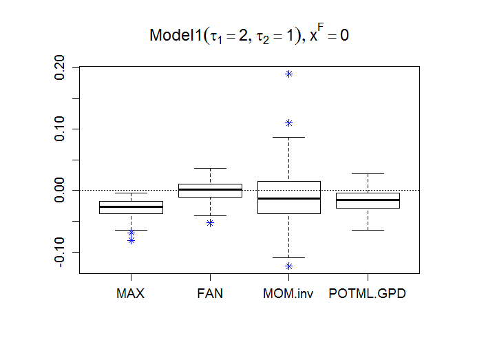
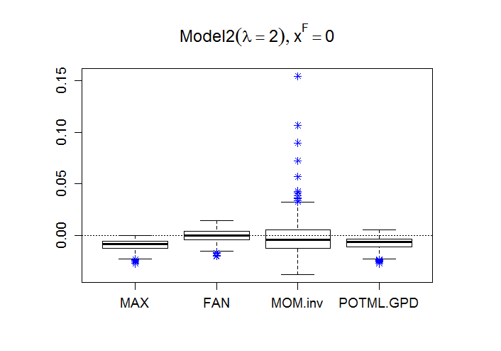
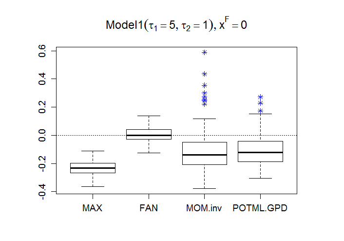
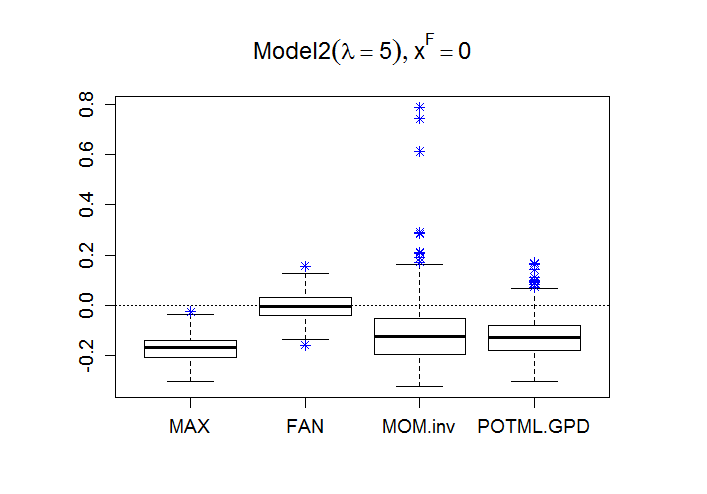
Figure 1: Boxplots of the optimal bias $\varepsilon(j,k^{*}_{0}),\,\,j=1,\ldots,N$, with $N=300$. Endpoint estimates are drawn from Model 1 (left) and Model 2 (right), with true value $x^{F}=x^{F_{1}}=x^{F_{2}}=0$.

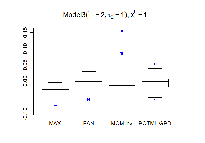
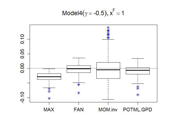
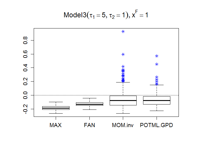
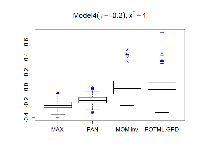
Figure 2: Boxplots of the optimal bias $\varepsilon(j,k^{*}_{0}),\,\,j=1,\ldots,N$, with $N=300$. Endpoint estimates are drawn from Model 3 (left) and Model 4 (right), with true value $x^{F}=x^{F_{3}}=x^{F_{4}}=1$.

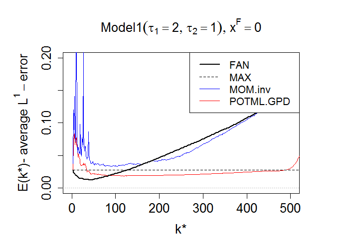
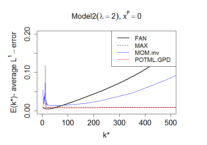
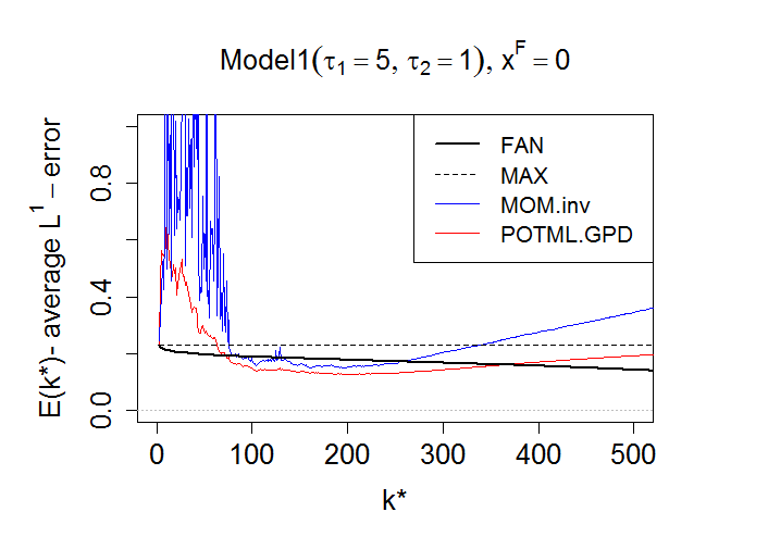
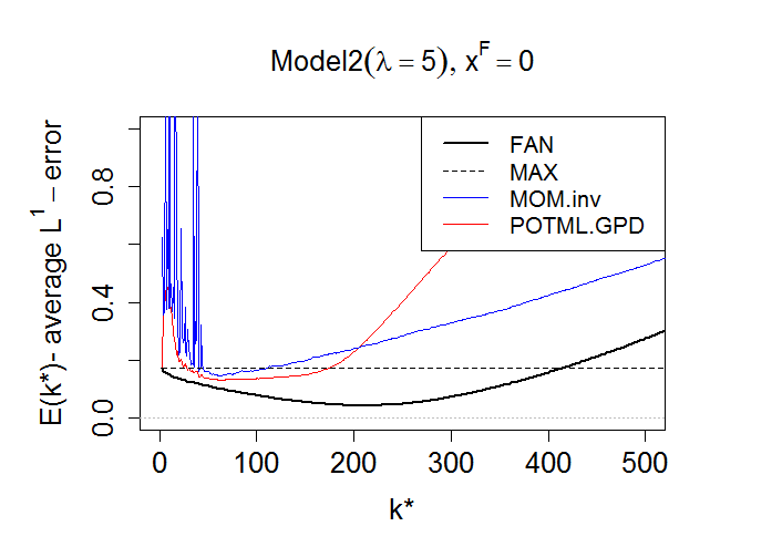
Figure 3: Average $L^{1}$-error, $E(k^{*})$, plotted against $k^{*}\leq n/2$. Endpoint estimates are drawn from Model 1 (left) and Model 2 (right), with true value $x^{F}=x^{F_{1}}=x^{F_{2}}=0$.

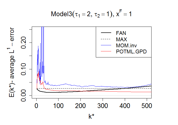
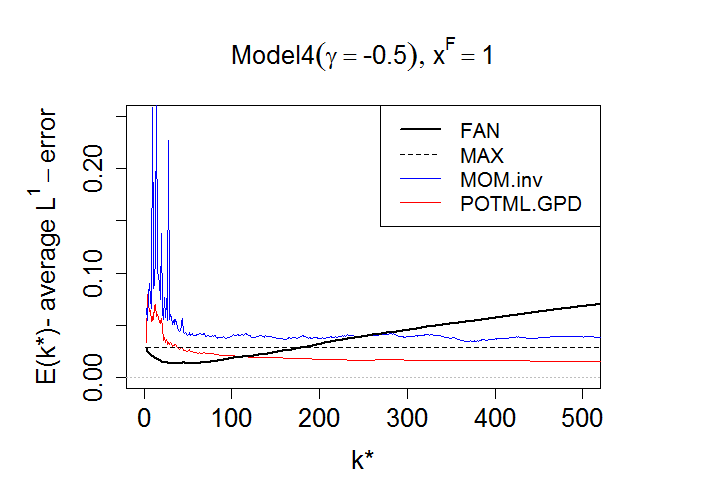
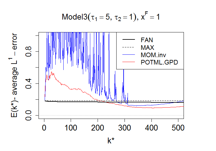
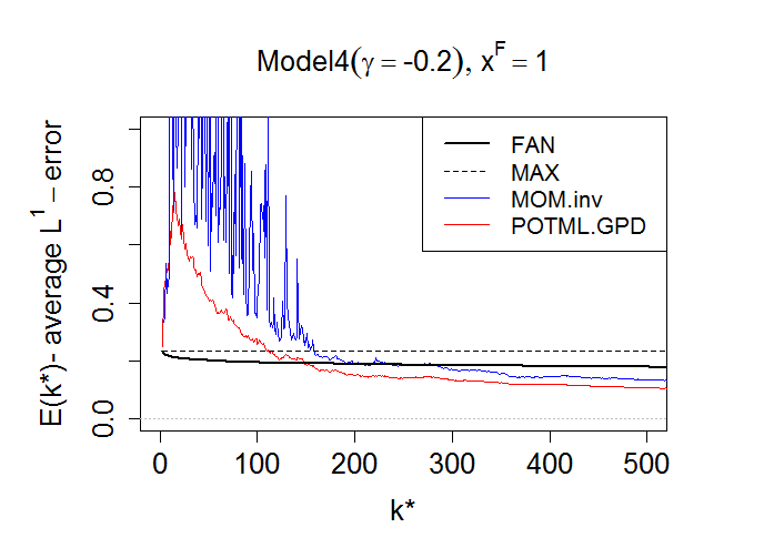
Figure 4: Average $L^{1}$-error, $E(k^{*})$, plotted against $k^{*}\leq n/2$. Endpoint estimates are drawn from Model 3 (left) and Model 4 (right), with true value $x^{F}=x^{F_{3}}=x^{F_{4}}=1$.

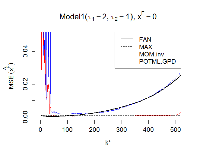
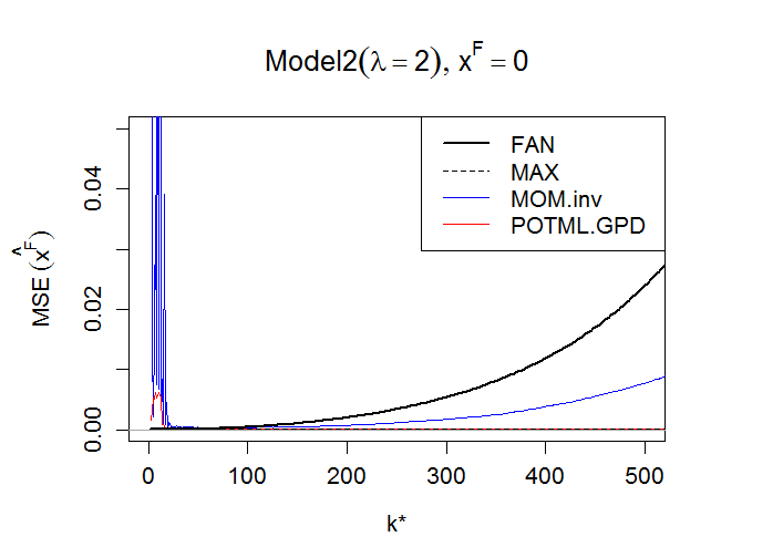
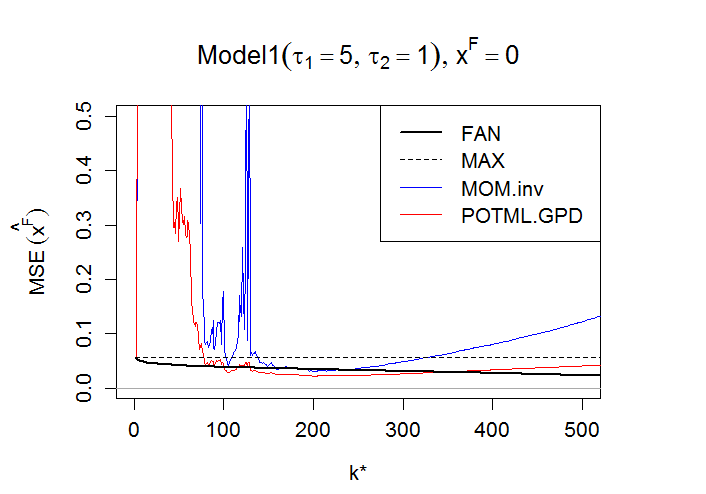
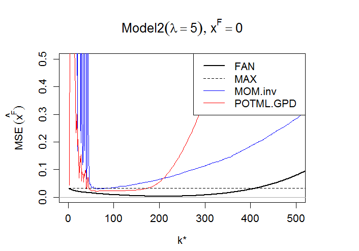
Figure 5: Mean squared error (MSE) as function of the number of upper o.s. $k^{*}$, $k^{*}\leq n/2$. Endpoint estimates are drawn from Model 1 (left) and Model 2 (right), with true value $x^{F}=x^{F_{1}}=x^{F_{2}}=0$.

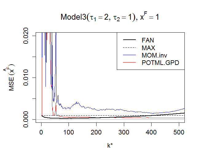
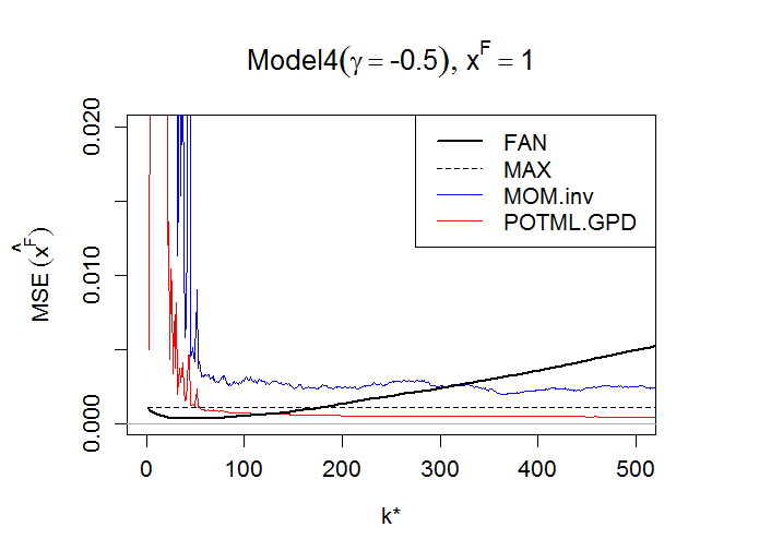
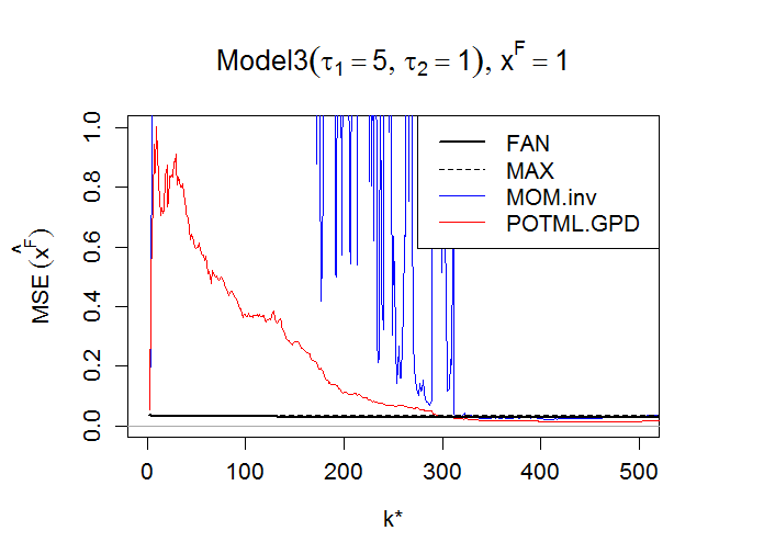
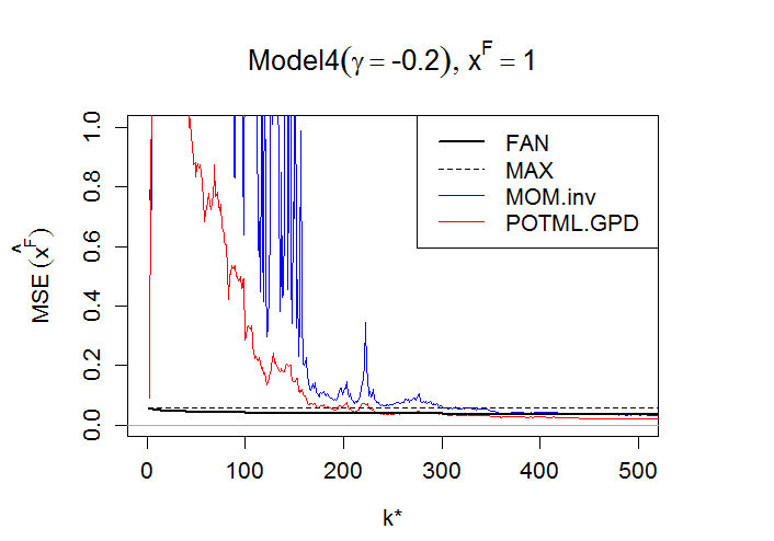
Figure 6: Mean squared error (MSE) as function of the number of upper o.s. $k^{*}$, $k^{*}\leq n/2$. Endpoint estimates are drawn from Model 3 (left) and Model 4 (right), with true value $x^{F}=x^{F_{3}}=x^{F_{4}}=1$.

Altogether, the general endpoint estimator FAN seems to be an improvement to the naïve MAX estimator and tends to surpass the MOM.inv and POTML.GPD estimators, by delivering low biased estimates quite often, while showing a low variance component. This is particularly true for a EVI close to zero, as it would be expected from the one estimator primarily tailored to tackle endpoint estimation in the Gumbel max-domain of attraction (cf. Fraga Alves and Neves,, 2014). Furthermore, the FAN estimator seems to work remarkably well under a fairly negative EVI, considering that this is a general estimator which does not accommodate any specific information about the true value of the EVI. The overall performance of the MOM.inv and POTML.GPD endpoint estimators is clearly damaged by their large variance in the top of the sample. It is worthy to notice that the presented estimation procedure $\hat{x}^{F}$ acts as a complement to numerical POTML methods for endpoint estimation, the latter only available for strict negative shape parameter $\gamma$; in contrast, $\hat{x}^{F}$ presents an explicit simple expression, unifying the estimation method to distributions with non-positive EVI, $\gamma\leq 0$.

4.2 A testing procedure built on the general endpoint estimator

This section concerns the finite sample performance of $G_{n,k}$, presented in Theorem 6, as a convenient tool for either discarding heavy-tailed models or for detecting short-tailed models $F\in{\mathcal{D}}(G_{\gamma})$, $\gamma<0$. One grounding result in this respect is that all the semi-parametric endpoint estimators we are adopting, are consistent under the assumption that $k=k_{n}$ is an intermediate sequence of positive integers, i.e. $k=k_{n}\rightarrow\infty$ and $k_{n}/n\rightarrow 0$, as $n\rightarrow\infty$. The testing procedures we wish to apply also bear on this usual assumption in statistics of extremes. There are many proposals for testing procedures aiming at the selection of a suitable max-domain of attraction. For a wide view on this topic, we refer the surveys on testing about extreme values conditions available in Hüsler and Peng, (2008) and Neves and Fraga Alves, (2008). We recall that EVI estimation is not a requirement for the general endpoint estimation defined (6) and emphasize that both Weibull and Gumbel domain are allowed. Thus, for the time being, we will rely on testing procedures which do not require external estimation of the EVI. We will compare the new test statistic $G_{n,k}$, defined in (16), with the Ratio and Greenwood statistics introduced in Neves et al., (2006) and Neves and Fraga Alves, (2007) for the one-side alternatives

$$H_{0}:F\in{\mathcal{D}}(G_{0})\qquad vs H_{1}:F\in{\mathcal{D}}(G_{\gamma})_{\gamma>0}$$

$$[\mbox{or } H_{1}^{\prime}:F\in{\mathcal{D}}(G_{\gamma})_{\gamma<0}]\,.$$

The Ratio(R) and Greenwood(Gr) statistics are defined as

$$R:=\frac{X_{n,n}-X_{n-k,n}}{N_{1}}\qquad Gr:=\frac{N_{2}}{\left(N_{1}\right)^{2}}\,\,,\\$$

with $N_{j}=N^{(j)}_{n,k}=\frac{1}{k}\sum_{i=0}^{k-1}\left(X_{n-i,n}-X_{n-k,n}\right)^{j},\,\,j=1,2$. Under $H_{0}$, the standardized version of Ratio statistic, $R^{*}:=R-\log k$, is asymptotically Gumbel, whereas the suitably normalized Greenwood statistic, $Gr^{*}:=\sqrt{k/4}(Gr-2)$, is asymptotically standard normal. Formally, approximated $\alpha$-significant tests against the alternative $H_{1}$ [resp. $H_{1}^{\prime}$] render the rejection regions $R^{*}\geq\omega_{1-\alpha}$ [resp. $R^{*}\leq\omega_{\alpha}$] and $Gr^{*}\geq z_{1-\alpha}$ [resp. $Gr^{*}\leq z_{\alpha}$], where $\omega_{\epsilon}:=\Lambda^{\leftarrow}(\epsilon)$ and $z_{\epsilon}:=\Phi^{\leftarrow}(\epsilon)$. Here, $\Phi$ denotes the d.f. of the standard normal. Corresponding $p$-values of the test are $p=1-\Lambda(g^{*})$ against the heavy-tailed alternative, and $p=\Lambda(g^{*})$ against the short-tailed alternative, for the observed values $r^{*}$ and $gr^{*}$ of the test statistics $R^{*}$ and $Gr^{*}$, respectively. The approximated $p$-values against heavy-tailed alternatives $H_{1}$ [resp. short-tailed alternatives $H_{1}^{\prime}$] are given by $1-\Lambda(r^{*})$ and $1-\Phi(gr^{*})$ [resp. $\Lambda(r^{*})$ and $\Phi(gr^{*})$], for an observed value $g^{*}:=g_{n,k}^{*}(0)$ of the test statistic $G_{n,k}^{*}(0)$.

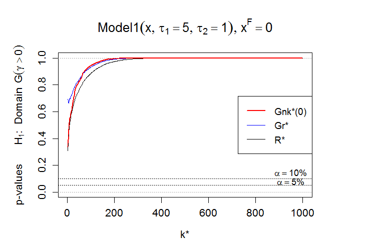
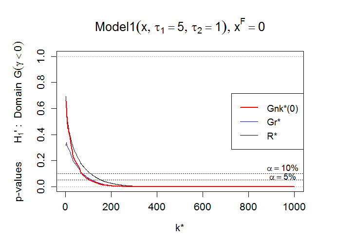
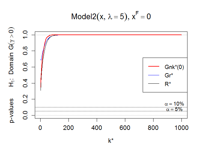
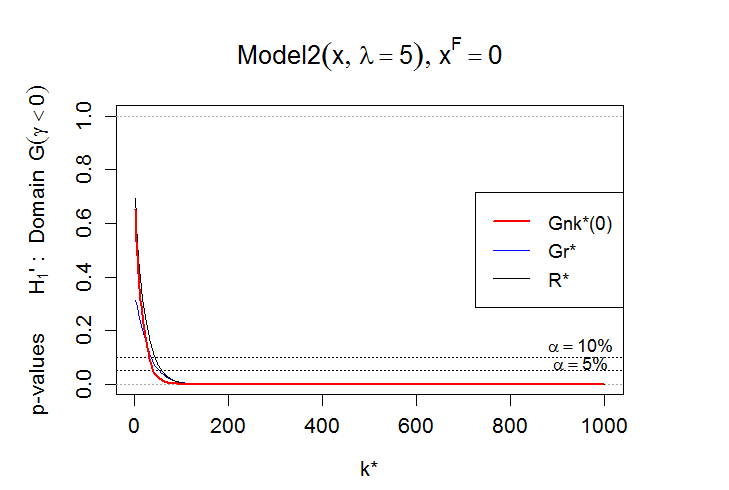
Figure 7: Average $p$-values of the simulated $G_{n,k}^{*}(0)$, $R^{*}$ and $Gr^{*}$ either against a heavy-tailed alternative (left) or a short-tailed alternative (right), with respect to $k^{*}\leq n\,=1000$.

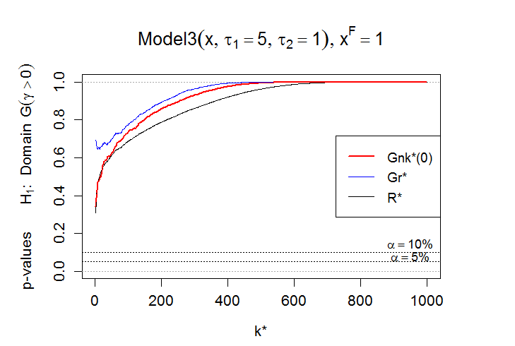
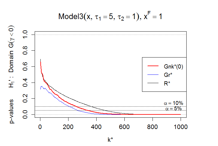
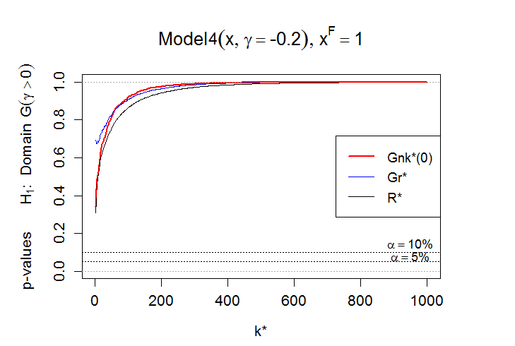
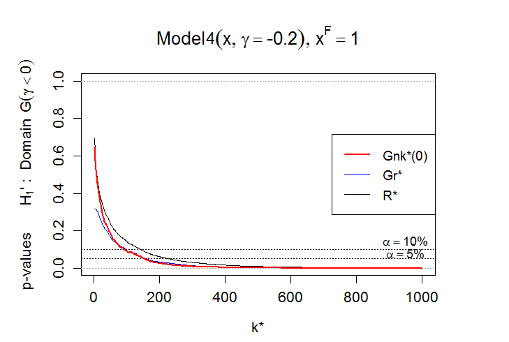
Figure 8: Average $p$-values of the simulated $G_{n,k}^{*}(0)$, $R^{*}$ and $Gr^{*}$ either against a heavy-tailed alternative (left) or a short-tailed alternative (right), with respect to $k^{*}\leq n\,=1000$.

Figures 7-8 summarize the comparison between the performance of the test based on $G_{n,k}^{*}(0)$ (cf. Theorem 6) with the above mentioned tests $R^{*}$ and $Gr^{*}$. The simulations yield large $p$-values in connection with the heavy-tailed alternatives $H_{1}$, meaning that heavy-tailed distributions are likely to be detected by these tests. On the opposite side, the test are not so sharp against short-tailed alternatives in $H_{1}^{\prime}$. The new test statistic $G_{n,k}^{*}(0)$ rejects on smaller values of $k^{*}$ than the $R^{*}$ statistic, thus revealing more powerful than the Ratio-test.

The Greenwood test compares favourably to $G_{n,k}^{*}(0)$ in terms of power, against the heavy-tailed alternative. However, it tends to be a more conservative test than the new proposal, often returning p-values much less than $5\%$.

5 Case study: supercentenarian women lifespan

This section is devoted to the practical illustration of our methodology for statistical inference about the endpoint. Our data set of oldest people comprises records of lifetimes in days of verified supercentenarians (women), with deaths in the time window 1986-2012. The data set was extracted from Table B of Gerontology Research Group (GRG), as of January 1, 2014, merged with Tables C and E, as of June 29, 2015, available at http://www.grg.org/Adams/Tables.htm. Although the referred database includes lifespan records tracing back to 1903, these are often sparse and with a low average number of yearly records, which is not surprising since the GRG was only founded in 1990. The later two years of records 2013-2014 are not yet closed. Therefore we settle with the $1272$ supercentenarian women lifetimes, recorded from 1986 to 2012, and corresponding to approximately $90\%$ of the total number of records since 1903.

The terms “life expectancy” and “lifespan” describe two entirely different concepts, although people tend to use these terms interchangeably. Life expectancy refers to the number of years a person is yet expected to live at any given age, based on the statistical average. Lifespan, on the other hand, refers to the maximum number of years that a person can potentially expect to live based on the greatest number of years anyone has lived. We are interested in the latter.

Formally, in gerontology literature, maximum lifespan potential (MLSP) is the operative definition for the verified age of the longest lived individual for a species (Olshansky et al., 1990b, ) and, in this sense, can be viewed as a theoretical upper limit to lifetime. The oldest documented age reached by any living individual is 122 years, meaning humans are said to have a MLSP of 122 years. In Biology, theories of ageing are mainly divided into two groups: damage theories and program theories. According to damage theories, we age because our systems break down over time; so, if damage theories hold true, we can survive longer by avoiding damaging our organism. Program theories consider that we age because there is an inbuilt mechanism that tells us to die; according to that, we cannot survive longer than the upper limit of longevity despite of our best efforts (see Hanayama, (2013)). Kaufmann and Reiss, (2007) also discussed the issue of whether the right endpoint of the life span is infinite, for which they analyzed mortality data from West Germany. Their estimated shape parameter within the Generalized Pareto model is equal to $-0.08$ and the right endpoint of the estimated beta distribution is equal to 122 years, an estimate that fits well to the worldwide reported life span of the most famous record-holder, the Frenchwoman Jeanne-Louise Calment (122 years and 164 days) who was born in Arles on Feb. 21, 1875 and died in Arles on Aug. 4, 1997. However, Kaufmann and Reiss, (2007) did not conclude categorically that human lifespan has a finite upper limit, arguing that by using the concept of penultimate distributions we can show that an infinite upper limit is well compatible with extreme value theory. They carry on pointing out a Beta distribution as a suitable model. Aarssen and de Haan, (1994) analyzed lifespan data from the Netherlands using statistical methods under the extreme value theory umbrella. Aarssen and de Haan, (1994) showed that there is a finite age limit, tackled with reasonable confidence bounds in the $113-124$ year span, a conclusion confined to the years of birth $1877-1881$ in the Netherlands.

Stephen Coles, a specialist in tracking human supercentenarians and co-founder of the Supercentenarian Research Foundation (SRF), refers to the supercentenarians as “the most extreme example of human longevity that we know about, the oldest old”. In Coles, (2011), the value 122 is referred to as the “Calment Limit” for human longevity (what is designated here as the MLSP), which is supported on the fact that nobody has come even close that extreme age over the last 19 years. It is also mentioned that, from his research experience, “supercentenarians had virtually nothing in common: they had different occupations, lifestyles, religions and so on, regardless the common factor of long-lived relatives.” Also, according to Vaupel, (2011) “the explosion in very long life has already begun”, although by his perspective “we cannot see much beyond 122.”

Several authors have stated that despite of the increasing “life expectancy”, the “maximum human lifespan” has not much changed. According to Troen and Cristafalo, (2001) some biodemographic estimates predict that elimination of most of the major diseases such as cancer, cardiovascular disease, and diabetes would add no more than 10 years to the average life expectancy, but would not affect MLSP (Olshansky et al., 1990a, ; Troen and Cristafalo,, 2001). Other researchers go further enough to hypothesize that mortality will be compressed against that fixed upper limit to life time (Compression Theory by Fries,, 1980). On the other hand, Wilmoth and Robine, (2003) argue a possible world trend in maximum lifespan, based on a long series of Swedish data. Above all, there is still plenty of scope to assess significance of other covariates, like the negative impact of obesity and epidemic diseases on the rise in life expectancy trends and the possible impact on the MLSP.

What researchers seem to agree on is the need for better data, since at present, there is insufficient data available on the extreme elderly population. We should keep in mind that age is often misreported and at the time the centenarians (and supercentenarians) were born, record keeping was less complete than it is nowadays.

With this illustrative example of estimation of the ultimate lifespan by adopting the general endpoint estimator, it is not our aim to make conclusions for a specific cohort of individuals in time or space, nor any other type of serial studies. Instead, the interest will be on the question of what are sensible bounds for the MLSP, at the current state of the art.

At this point, several assumptions are needed about the right tail of the lifetime distribution, which is the focus of our extreme value analysis. The first assumption is that the available data comprises a sample of i.i.d. observations. We find reasonable to assume independence in our data, since we have one record for each individual person. The stationarity assumption is preliminary asserted from the plot in Figure 9 displaying the comparative boxplots for the larger women’s lifetimes by the year. A common feature to all the boxplots is the presence of very large observations classified as extreme outcomes. The boxplots also suggest an increasing third quartile as we progress in time. Such an increase is not so apparent in the annual maxima as we move across the $27$ time points (years). A possible interpretation is that an increase in the mean of the supercentenarians’ lifetimes may not be connected to an increasing lifespan over time, but rather to a possible trend in the frequency of the highest lifetime observations. There is a recent semi-parametric development by de Haan et al., (2015), suitable for assessing the presence of a trend in the frequency of extreme observations, which is also reflected in the scale of extremes. However, their inference techniques require a large number of replicates per year, and this is not at our grasp given the limited amount of observations available within the same year. For instance in the top part of Figure 9, that we have always less than 40 yearly observations until 1997 (the year of Calment), with the lowest number of 12 observations for 1991. Although the number of observations virtually doubles for the later years, the absolute record still stands on the Calment limit of 122 years, the overall sample maximum. The plot in Figure 10 shows the Loess fit (Local scatterplot smoothing) to the yearly data, given by blue curve overlay. This is almost parallel to the horizontal axis. Confidence bands are also presented with a preassigned 95% confidence level. These seem rather narrow. Hence, we find no evidence of a particular trend through this nonparametric technique.

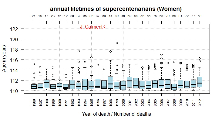
Figure 9: Comparative boxplots of the lifetimes of supercentenarians (Women) reported from 1986 to 2012.

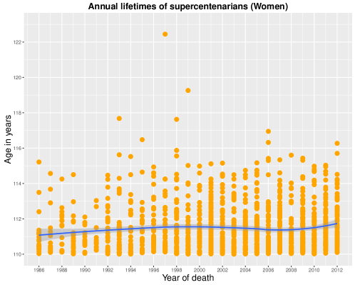
Figure 10: Loess fit to the lifetime of supercentenarians (Women) reported from 1986 to 2012.

Despite the above, a POT parametric approach is applied to detect a possible trend in the scale. Here, the GPD is fitted to the threshold excesses, via a ML fit to $H_{\gamma}(x/\sigma)$, GPD is fitted to the threshold excesses, considering a trend through time as $\sigma=\sigma_{t}=\exp\{\beta_{0}+\beta_{1}\,t\}$. The resulting non-stationary model is denoted by $\mathcal{M}_{1}$, whereas the corresponding stationary version GPD with $\sigma=\exp\{\beta_{0}\}$ is denoted by $\mathcal{M}_{0}$. Let $\ell_{1}$ and $\ell_{0}$ be the maximized log-likelihoods for models $\mathcal{M}_{1}$ and $\mathcal{M}_{0}$, respectively. The Likelihood Ratio test for $H_{0}:\mathcal{M}_{1}=\mathcal{M}_{0}$ using the deviance statistic $D=2\{\ell_{1}-\ell_{0}\}$ to formally compare models $\mathcal{M}_{1}$ and $\mathcal{M}_{0}$, returns the results summarized in Table 2, for the lifetime data over the selected thresholds $110,111,112,113$ and $114$. The last column contains the $p$-values, related to the different threshold selection. Again, we find no strong evidence of a linear trend in the log-scale parameter $\sigma$. Moreover, for each threshold, the EVI and endpoint ML estimates for women lifetimes are also listed for the sake of comparison with subsequent results in Section 5.3.

Table 2: Maximum-likelihood parametric GPD($\sigma_{t}$) and GPD($\sigma$) fit to the lifetime exceedances of supercentenarian women for the time period 1986-2012.

$\sigma_{t}$	$\ell_{i}$, $i=0,1$	$\hat{\beta}_{0}$	$\hat{\beta}_{1}$	$\hat{\gamma}$	thresh$/\#$exc	$\hat{x}^{F}_{POT}$	$p$-value
$\exp\{\beta_{0}+\beta_{1}\,t\}$	-1739.324	0.327	0.006	-0.056	110/1272
$\exp\{\beta_{0}\}$	-1740.238	0.432	–	-0.061		135.36	0.1763
$\exp\{\beta_{0}+\beta_{1}\,t\}$	-867.215	0.497	-0.003	-0.083	111/639
$\exp\{\beta_{0}\}$	-867.374	0.436	–	-0.078		130.63	0.5729
$\exp\{\beta_{0}+\beta_{1}\,t\}$	-424.197	0.558	-0.013	-0.062	112/338
$\exp\{\beta_{0}\}$	-425.542	0.304	–	-0.045		142.05	0.1010
$\exp\{\beta_{0}+\beta_{1}\,t\}$	-192.652	0.567	-0.019	-0.044	113/164
$\exp\{\beta_{0}\}$	-193.942	0.198	–	-0.016		191.21	0.1083
$\exp\{\beta_{0}+\beta_{1}\,t\}$	-75.904	0.150	-0.021	0.141	114/82
$\exp\{\beta_{0}\}$	-76.495	-0.237	–	0.170		–	0.2769

The previous preliminary parametric analysis does not exhaust all the possible choices of parametric models encompassing a trend in extremes. The interest is not in the selection of the most suitable parametric model for extremes, but in being able to ascertain, with a certain degree of confidence, that dropping out of the time covariate does not affect our subsequent analysis under the assumption of stationary supercentenarian women’s lifetimes. For recent applications incorporating information over time, we refer the works of Stephenson and Tawn, (2013) and de Haan et al., (2015). The latter comprises a comparative analysis with existing methodologies in a similar context.

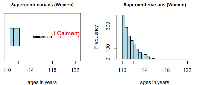
Figure 11: Boxplot and histogram built on the lifetimes of supercentenarian women, for the time interval 1986-2012.

The available supercentenarian women data should be regarded as the greatest lifetimes collection ever attained by the human population. We have $1272$ observations available, which we have found to satisfy the i.i.d. assumption. Figure 11 contains the boxplot and the histogram for the whole univariate data set.

5.1 Testing finiteness in the right endpoint

Our first aim is to assess finiteness in the right endpoint of the d.f. $F$ underlying the women lifespan data. The detection of a possibly finite upper bound on our data follows a semiparametric approach, meaning that we essentially assume that $F$ belongs to some max-domain of attraction. We then consider the usual asymptotic setting, where $k=k_{n}\rightarrow\infty$ and $k_{n}/n\rightarrow 0$, as $n\rightarrow\infty$, and hence $X_{n-k,n}\rightarrow x^{F}\;a.s.$ According to this setting, it is only natural to expect that any statistical approach to the problem of whether there is a finite endpoint or not, will depend on the extent of the dip into the original sample of supercentenarian women’s records. The baseline to this issue is mostly driven by a second and more operative question: how to select the adequate top sample fraction to use with both our testing and estimation methods? A suitable choice of $k$ comes from a similar approach to the one in Wang, (1995), where $k_{opt}$ is deemed to be selected at the value $k$ from which the null hypothesis is rejected.

For a more definite judgment about the existence of a finite upper bound on the supercentenarian lifetimes, we are going to apply the testing procedure introduced in Neves and Pereira, (2010). The purpose now is to detect finiteness in the right endpoint of the underlying distribution which may belong to either Weibull or Gumbel domains. More formally, the testing problem

$$H_{0}:F\in{\mathcal{D}}(G_{0}),\,x^{F}=\infty\quad vs\quad H_{1}:F\in{\mathcal{D}}(G_{\gamma})_{\gamma\leq 0},\,x^{F}<\infty$$

is tackled using the log-moments $N_{r}\equiv N_{n,k}^{(r)},\,\,r=1,2$, defined in (21), but now replacing the observations $X_{i,n}$ by their log-transform $\log(X_{i,n})$. It is possible to do so because we are dealing with positive observations. We point out however that this leads to a non-location invariant method. The test statistic $T_{1}$ being used is defined as

$$T_{1}:=\frac{1}{k}\sum_{i=1}^{k}\frac{X_{n-i,n}-X_{n-k,n}-T}{X_{n,n}-X_{n-k,n}},\mbox{ with }T:=X_{n-k,n}\frac{N_{1}}{2}\left(1-\frac{\left[N_{1}\right]^{2}}{N_{2}}\right)^{-1}\,.$$

Under $H_{0}$ the standardized version of the test, $T_{1}^{*}:=\sqrt{k}\,\log k\,T_{1}$, is asymptotically normal. Moreover, $T_{1}^{*}$ tends to inflect to the left for bounded tails in the Weibull domain and to the right if the underlying distribution belongs to the Gumbel domain. The rejection region of the test is given by $|T^{*}_{1}|\geq z_{1-\alpha/2}$, for an approximate $\alpha$ significance level. Figure 12 displays the sample path of $T_{1}^{*}$. The most adequate choice of the intermediate number $k$ (which carries over to the subsequent semi-parametric inference) is set on the lowest $k$ at which the critical barriers with a $\alpha=5\%$ significance level are crossed. This optimality criterium yields $k_{0}^{NP}=487$, spot on the smallest value where we find enough evidence of a finite endpoint.

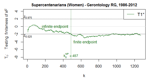
Figure 12: Detecting finiteness in right endpoint for verified supercentenarians data set: sample paths of the normalized statistics. The horizontal dashed lines correspond to the $\alpha=5\%$ critical barriers.

It remains to be assess whether the distribution underlying the supercentenarian data (now assumed bounded from above) belongs to the Gumbel domain or to the Weibull max-domain of attraction. This will be carried out by a proper hypothesis-testing problem, termed statistical choice of extremes domains. In view of our specific interest on the finite endpoint, we are using the one-sided version of the test. The hypotheses are:

$$H_{0}:F\in{\mathcal{D}}(G_{0})\quad vs\quad H_{1}^{\prime}:F\in{\mathcal{D}}(G_{\gamma})_{\gamma<0}\,\,.$$

Figure 13 depicts the sample paths of the new test statistic $G_{n,k}^{*}(0)$ from Theorem 6, the Greenwood $Gr^{*}$ statistic, and the Ratio $R^{*}$ statistic, as well as their $\alpha=5\%$ asymptotic critical values. The Greenwood test finds enough evidence to reject the Gumbel domain hypothesis in favour of a bounded short-tail in Weibull domain, at the suitable intermediate value of $k_{0}^{G}=465$. The two other statistics, new $G_{n,k}^{*}(0)$ and ratio $R^{*}$, lead to a more conservative conclusion, with both tests leaning towards the non rejection of the null hypothesis. This conservative aspect also crops up in the simulations section (Section 4), where the Greenwood test is found to be more powerful against short-tailed alternatives attached to $\gamma<0$.

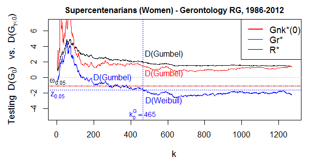
Figure 13: Testing max-domains of attraction with short tailed alternative, for verified supercentenarians data set: sample paths of the normalized test statistics. The horizontal dashed lines correspond to the $\alpha=5\%$ critical barriers.

From the previous analysis, we find it reasonable to assume a finite right endpoint for some distribution in the Weibull domain simultaneously for all the adopted testing methods at the maximum number of upper extremes

$$k_{opt}:=\max\{k_{0}^{G},k_{0}^{NP}\}=487.$$

Therefore, based not only on the testing procedures but also on the complementary EVI estimation presented in Section 5.3, it seems reasonable to conclude that the lifespan distribution belongs to the Weibull domain of attraction with finite right endpoint $x^{F}$.

For definitely discarding the presence of a heavy-tailed distribution underlying our data set, it is also important to test:

$$H_{0}:F\in{\mathcal{D}}(G_{0})\quad vs\quad H_{1}:F\in{\mathcal{D}}(G_{\gamma})_{\gamma>0}\,.$$

In Figure 14 we observe that all the $p$-values determined by all the three test statistics are increasing with $k$. Again, the conservative behavior of the two tests seems to emerge. Despite all $p$-value paths begin at very small values around zero, this only lingers for a tight range of higher thresholds which may not be in good agreement with the requirement of a sufficiently large $k$. The Greenwood statistic returns $p$-values very close to 1, from about $k=400$ onwards. The other two statistics ($G_{n,k}^{*}(0)$ and $R^{*}$) yield moderate $p$-values, with larger values returned by $G_{n,k}^{*}(0)$. It seems sensible then to discard a heavy-tailed distribution for the supercentenarian women lifespan, a conclusion clearly verified by the Greenwood test.

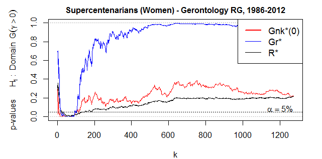
Figure 14: Testing max-domains of attraction for verified supercentenarians data set: $p$-values for the normalized test statistics, with heavy tailed alternatives. The horizontal dashed line corresponds to the $\alpha=5\%$ nominal level.

5.2 Endpoint estimation for women’s records without EVI knowledge

Following the testing procedures in 5.1 and the reported optimal number $k_{opt}=487$, we will present analogous graphical tools with respect to endpoint estimation. The first purpose is to illustrate the smooth behaviour of $\hat{x}^{F}$ defined in (6), already anticipated in the simulations section (Section 4).

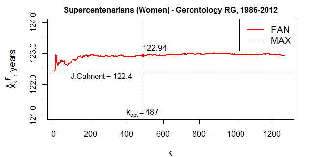
Figure 15: Endpoint estimation for verified supercentenarians data set: estimator $\hat{x}^{F}$ and Calment limit.

Figure 15 displays the comparative finite-sample behaviour of $\hat{x}^{F}$ (notation: FAN) with the naïve Calment limit (notation: MAX) for the supercentenarian’s data set. Recall that our database is regarded as a collection of the greatest lifetimes of women population and that the general endpoint estimator $\hat{x}^{F}$ always returns values above the naïve endpoint estimate, i.e. greater than “Calment limit” of $122.4$ years.

After the initial rough path in the range of approximately one hundred top observations, the estimates trajectory of $\hat{x}^{F}$ then becomes very flat. Once we dip into the intermediate range of extremes, the sample path becomes smoother.

At this point we find it sensible to provide similar information provided by the other semi-parametric and parametric endpoint estimators already intervening in the simulation study, as they constitute a good complement to a more thorough insight about the true endpoint. This is the subject of the next section.

5.3 Linking endpoint estimation of women’s records to EVI estimation

In this section, the endpoint estimation is tackled using methodologies that require an estimator for the extreme value index $\gamma<0$. In this sequence, we adopt the moment related estimator $\hat{\gamma}_{n,k}^{-}$ (notation: MOM.inv), defined in (19), and the POTML.GPD estimator of the shape parameter $\hat{\gamma}_{n,k}^{ML}$ to plug in (23) (subject to $\gamma<0$). Figure 16 is the estimates plot of the chosen estimators for $\gamma$, as function of $k$. We note that these two estimators enjoy the location and scale invariance property. Retaining the $k_{opt}=487$ larger observations (a value delivered by the testing procedures) as the effective sample, we find the point estimates $\hat{\gamma}_{n,487}^{-}=-0.087$ and $\hat{\gamma}_{n,487}^{ML}=-0.059$, both coherent with a short-tailed distribution attached to some $\gamma\in(-1/2,0)$.

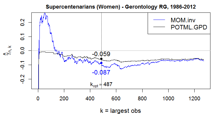
Figure 16: EVI estimation with the verified supercentenarian data.

Figure 17 depicts the results for estimators $\hat{x}^{F}_{ML}$, $\hat{x}^{*}$ (defined in (23) and (18), respectively). We are also including the second order reduced bias version of the general endpoint estimator $\hat{x}^{F}_{RB2}$ defined in (13), by plugging in the estimators $\hat{\gamma}=\hat{\gamma}^{-}_{n,k}$ and $\hat{a}_{0}\bigl{(}\frac{n}{k}\bigr{)}$ provided in (19) and (20), respectively. The trajectory of $\hat{x}^{F}_{RB2}$ lies in the middle range between that of $\hat{x}^{F}_{ML}$ and of $\hat{x}^{*}$.

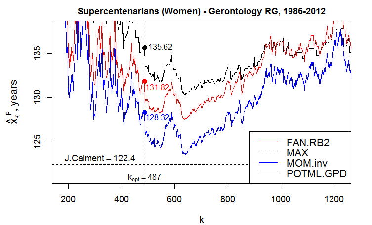
Figure 17: Endpoint estimation with the verified supercentenarian data.

The optimal value $k_{opt}=487$ can viewed as benchmark value (or change point) since it breaks the disruptive estimates pattern. It actually pinpoints where the graph stops being too rough to make inference and starts being more stable, so that we can infer about the endpoint. The latter applies in particular to estimators $\hat{x}^{*}$, $\hat{x}^{F}_{RB2}$ and $\hat{x}^{F}_{ML}$, which return $\hat{x}^{*}_{k_{opt}}=128.32$, $\hat{x}^{F}_{RB2,k_{opt}}=131.82$ and $\hat{x}^{F}_{ML,k_{opt}}=135.62$. The simulations also outline the plain general endpoint estimator $\hat{x}^{F}$ as being relatively efficient (in terms of bias and MSE) on those moderate values of $k^{*}$ where other estimators fall short. In this respect, Figure 15 shows a rather flat plateau from which we find safe to draw an estimate for the endpoint, and this portion of the graph includes $\hat{x}^{F}_{k_{opt}}=122.94$. The asymptotic results in Theorem 4 for $\gamma\in(-1/2,0)$ equip us with a tool for finding an approximate $100(1-\alpha)\%$ upper bound for the true endpoint $x^{F}$. Obviously, this process calls for the estimation of $\gamma$ since we need some guidance about the proper interval where the EVI lies within. Hence, we have just introduced the most direct link to the estimation of $\gamma$ (see Figure 16) in connection with the general endpoint estimator $\hat{x}^{F}$. Selecting $k_{opt}=487$, the $95\%$ confidence upper bound for $x^{F}$ delivered by (14) is $133.23$ years.

We also note that the simulation outcomes relate well to the present results arising from the available data of supercentenarian women’s records. For instance, we observe in Figure 16 that small values of $k$ ($k\leq 110$, approximately) find positive estimates for the MOM.inv estimator which could on their own account for the erratic pattern of $\hat{x}^{*}_{k}$ in the plot of Figure 17, but the simulations have yield this rough pattern very often in connection with a true negative EVI. Furthermore, the shape parameter $\gamma$ is estimated via POTML subject to $\gamma<0$ (cf. Figure 16) and this returns endpoint estimates $\hat{x}^{F}_{ML}$ well aligned with the ones pertaining to $\hat{x}^{F}_{RB2}$ and $\hat{x}^{*}_{k}$ (cf. Figure 17). Therefore, heeding to the simulation results, we find reasonable to conclude that the misrepresentation of the negative EVI for moderate values of $k$ is not the main factor compromising the performance of the adopted endpoint estimators in the early part of the plot (amounting to about $10\%$ of the original sample size $n$, say).

Finally, this practical application also seems to suggest that removing the bias component from $\hat{x}^{F}$ causes an increase in the variance. The bias/variance trade-off effect is grasped more thoroughly in the Appendix 8, where the finite sample properties of the second order reduced bias estimator $\hat{x}^{F}_{RB2}$ are studied by taking Models 1 and 4, from Section 4, as parent distributions. The brief simulation study in the Appendix 8 is expected to reinforce the suggested competitive performance amongst the above-mentioned endpoint estimators.

5.4 An upper limit to lifespan and probability of surpassing Calment limit

From the previous data analysis, one would say that the ultimate human lifespan would not be greater than 133.23 years (the estimated upper bound from (14), obtained in section 5.3). This gives some insight beyond Calment’s achievement: the absolute record of 122.4 years, still holding to the present date (for the last 19 years). We thus expect that the probability of exceeding the “Calment limit”, even for a supercentenarian women, will be extremely low.

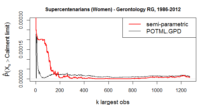
Figure 18: Probability of exceeding the “Calment limit”, for a supercentenarian women, given today’s state of the art.

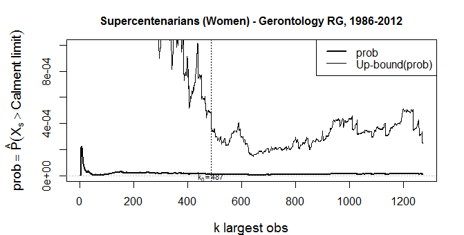
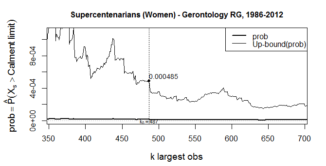
Figure 19: Probability of exceeding the “Calment limit” using the POTML.GPD approach and corresponding $95\%$ confidence bound: all sample (top); $350\leq k\leq 700$ (bottom).

This tail probability can be estimated using the following semi-parametric estimator:

$$\widehat{P}_{n}(X_{s}>122.4):={k\over n}\left\{\max\left(0,1+\hat{\gamma}_{n,k}^{-}{122.4-X_{n-k,n}\over\hat{a}(n/k)}\right)\right\}^{-1/\hat{\gamma}_{n,k}^{-}},$$ (24)

(cf. (4.4.1) in de Haan and Ferreira,, 2006) where $X_{s}:=X|X\geq 110$ denotes the lifetime of a supercentenarian women, and $\hat{\gamma}_{n,k}^{-}$, $\hat{a}(n/k)$ are the related estimators defined in (19) and (20), respectively.

Figure 18 depicts the probability estimates from (24), together with their POTML.GPD analogues, for a wide range of larger values of the 1272 verified supercentenarians data set. In contrast with the previous statistical analysis, the sample size $n$ now intervenes in (24). Therefore, any inference drawn on this account will apply to the subpopulation of supercentenarian women under study. All point estimates are very close to zero. Figure 19 displays again the POTML.GPD estimates but with respective $95\%$ upper bounds. Since we are dealing with very small probabilities the asymptotic bounds are not so sharp, as opposed to the case of an underlying distribution with infinite right endpoint.

6 Concluding remarks

The scope for application of the right endpoint estimator introduced in Fraga Alves and Neves, (2014), primarily designed for the Gumbel domain of attraction, is here extended to the case of an underlying distribution function $F$ in the Weibull domain. The consistency property and asymptotic distribution of this general endpoint estimator $\hat{x}^{F}$ renders a unified estimation procedure for the right endpoint under the assumption that $F\in\mathcal{D}(G_{\gamma})_{\gamma\leq 0}$. A new test statistic arises tied-up with $\hat{x}^{F}$ thus incrementing the range of available testing procedures for selecting max-domains of attraction. Our main findings are listed below.

• The general endpoint estimator does not require the estimation of the EVI, unlike the widely-used semi-parametric alternatives.

• By construction, the estimator $\hat{x}^{F}$ always returns larger values than the sample maximum $X_{n,n}$, a property not shared by other semi-parametric methodologies we have encountered so far, particularly those predicated on the Weibull max-domain of attraction.

• The simulation study conveys a good finite sample performance of the general endpoint estimator, ascertaining competitiveness to benchmark endpoint estimators specifically tailored for the Weibull domain.

• Related to the previous, the general endpoint estimator performs better for distributions with some $\gamma>-1/2$, which corresponds to the most common situation in practical applications.

• The problem of choosing the most adequate number $k$ of upper order statistics is here mitigated by the usual flat pattern of the estimates trajectories, a typical feature of the general endpoint estimator.

• The application to the supercentenarian women’s lifetimes illustrates how we can easily establish a confidence upper bound to the right endpoint, building on the asymptotic results for $\gamma>-1/2$.

7 APPENDIX A: Proofs

This section is entirely dedicated to the proofs of the results introduced in Section 3. In what follows we find more convenient to consider the estimator $\hat{x}^{F}$ in the functional form

$$\hat{x}^{F}=X_{n-k,n}-\frac{1}{\log 2}\int_{0}^{1}\bigl{(}X_{n-[2ks],n}-X_{n-[ks],n}\bigr{)}\,\frac{ds}{s},$$ (25)

where $[a]$ denotes the integer part of $a\in{\mathbb{R}}$ (more details about the representation (25) can be obtained in Fraga Alves and Neves,, 2014).

We note that if $s\in[0,\,1/(2k)[$, then the integral in (25) is equal to zero. Bearing this in mind, we write

$$\hat{x}^{F}=X_{n-k,n}-\frac{1}{\log 2}\int_{\frac{1}{2k}}^{1}\bigl{(}X_{n-[2ks],n}-X_{n-[ks],n}\bigr{)}\,\frac{ds}{s}.$$

Moreover, if $s\in[1/(2k),1/k[$ then $[ks]=0$ (not depending on $s$) and thus $X_{n-[ks],n}=X_{n,n}$. Therefore, we have that

$$\hat{x}^{F}=X_{n-k,n}-\frac{1}{\log 2}\Bigl{\{}\int_{\frac{1}{2k}}^{\frac{1}{k}}X_{n-[2ks],n}\,\frac{ds}{s}-X_{n,n}\,\int_{\frac{1}{2k}}^{\frac{1}{k}}\frac{ds}{s}+\int_{\frac{1}{k}}^{1}(X_{n-[2ks],n}-X_{n-[ks],n})\,\frac{ds}{s}\Bigr{\}}.$$ (26)

With a suitable variable transform on the last integral, we can reassemble (26) in a tidy manner:

$$\hat{x}^{F}=X_{n,n}+X_{n-k,n}-\frac{1}{\log 2}\int_{\frac{1}{2}}^{1}X_{n-[2ks],n}\,\frac{ds}{s}.$$ (27)

This is the main algebraic expression that will be used to derive the asymptotic distribution of $\hat{x}^{F}$ in the proof of Theorem 2, which is a natural consequence of the three random contributions in (27).

Proof of Proposition 1: We see that the integral in the functional form (27) satisfies the inequalities

$$(\log 2)\,X_{n-k,n}\leq\int_{\frac{1}{2}}^{1}X_{n-[2ks],n}\,\frac{ds}{s}\leq(\log 2)\,X_{n-2k,n}.$$

Therefore, we obtain the following upper and lower bounds involving $\hat{x}^{F}-x^{F}$,

$$X_{n,n}-x^{F}\,\leq\,\hat{x}^{F}-x^{F}\,\leq\,(X_{n,n}-x^{F})+X_{n-k,n}-X_{n-2k,n},$$

and the result thus follows easily because the three o.s. $X_{n,n}$, $X_{n-k,n}$ and $X_{n-2k,n}$ all converge almost surely to $x^{F}$, provided the intermediate nature of $k=k_{n}$. ∎

Remark 7.

Alternative proof based on the functional form (7) of the $k^{*}:=2k$ top o.s.: strong consistency of the general endpoint estimator comes from the lower and upper bounds of (7) given below.

$$\hat{x}^{F}-x^{F} = (X_{n,n}-x^{F})+\left(X_{n-k,n}-\frac{1}{\log 2}\sum_{i=0}^{k-1}\log(\frac{k+i+1}{k+i})\,X_{n-k-i,n}\right)$$

$$\geq (X_{n,n}-x^{F})+\left(X_{n-k,n}-X_{n-k,n}\,\frac{1}{\log 2}\sum_{i=0}^{k-1}\log(\frac{k+i+1}{k+i})\right)=X_{n,n}-x^{F}$$

and on the other hand,

$$\hat{x}^{F}-x^{F} \leq (X_{n,n}-x^{F})+\left(X_{n-k,n}-X_{n-2k+1,n}\,\frac{1}{\log 2}\sum_{i=0}^{k-1}\,\log(\frac{k+i+1}{k+i})\right)$$

$$= (X_{n,n}-x^{F})+(X_{n-k,n}-X_{n-2k+1,n})\,\,;$$

since for any intermediate $k=k_{n}$ the o.s. $X_{n,n},X_{n-k,n},X_{n-2k,n}$ converge almost surely to $x^{F}$, the result follows.

Before getting under way to the proof of the main Theorem, we need to lay down some ground results. These comprise a Proposition regarding $\gamma<0$ and a Lemma for general $\gamma$.

Proposition 8.

Suppose $X_{n,n}$ is the maximum of a random sample whose parent d.f. $F$ detains finite right endpoint of $F$, i.e. $x^{F}=U(\infty)<\infty$. Assume the second order condition (8) holds with $\gamma<0$. If $k=k_{n}$ is such that, as $n\rightarrow\infty$, $k\rightarrow\infty$, $k/n\rightarrow 0$ and $\sqrt{k}\,A_{0}(n/k)\rightarrow\lambda^{*}\in{\mathbb{R}}$, then

1. for $\gamma\geq-1/2$, for each $\varepsilon>0$,

   $$k^{-\gamma-\varepsilon}\biggl{|}\frac{X_{n,n}-x^{F}}{a_{0}\bigl{(}\frac{n}{k}\bigr{)}}\biggr{|}\,\,\displaystyle{\mathop{\longrightarrow}_{n\rightarrow\infty}^{p}}\,0.$$ (28)

   Moreover,

   $$k^{-\gamma}\,\frac{X_{n,n}-x^{F}}{a_{0}\bigl{(}\frac{n}{k}\bigr{)}}\,\,\displaystyle{\mathop{\longrightarrow}_{n\rightarrow\infty}^{d}}\,\,\frac{Z^{\gamma}}{\gamma},$$

   where $Z$ denotes a standard Fréchet with d.f. $\Phi_{1}$ as in (2).

2. for $\gamma<-1/2$,

   $$\sqrt{k}\,\biggl{|}\frac{X_{n,n}-x^{F}}{a_{0}\bigl{(}\frac{n}{k}\bigr{)}}\biggr{|}\,\,\displaystyle{\mathop{\longrightarrow}_{n\rightarrow\infty}^{p}}\,0.$$

Proof: Owing to the well-known equality in distribution that $X_{i,n}\displaystyle{\mathop{=}^{d}}\,U(Y_{i,n})$, $i=1,2,\ldots,n$, with $\bigl{\{}Y_{i,n}\bigr{\}}_{i=1}^{n}$ the $n$-th o.s. from a sample of $n$ independent r.v.s with common (standard) Pareto d.f. given by $1-x^{-1}$, $x\geq 1$, then the following equality in distribution holds:

$$\frac{X_{n,n}-x^{F}}{a_{0}\bigl{(}\frac{n}{k}\bigr{)}}\,\displaystyle{\mathop{=}^{d}}\,\Bigl{\{}\frac{U\bigl{(}\frac{k}{n}Y_{n,n}\,\frac{n}{k}\bigr{)}-U\bigl{(}\frac{n}{k}\bigr{)}}{a_{0}\bigl{(}\frac{n}{k}\bigr{)}}+\frac{1}{\gamma}\Bigr{\}}-\Bigl{\{}\frac{U(\infty)-U\bigl{(}\frac{n}{k}\bigr{)}}{a_{0}\bigl{(}\frac{n}{k}\bigr{)}}+\frac{1}{\gamma}\Bigr{\}}.$$

Now we use conditions (8) and (10) with $t$ replaced by $n/k$ everywhere:

$$\frac{X_{n,n}-x^{F}}{a_{0}\bigl{(}\frac{n}{k}\bigr{)}} \displaystyle{\mathop{=}^{d}} \biggl{\{}\frac{k^{\gamma}\bigl{(}n^{-1}Y_{n,n}\bigr{)}^{\gamma}-1}{\gamma}+\frac{1}{\gamma}+A_{0}\bigl{(}\frac{n}{k}\bigr{)}\Psi^{\star}_{\gamma,\rho}\Bigl{(}\frac{k}{n}\,Y_{n,n}\Bigr{)}\bigl{(}1+o_{p}(1)\bigr{)}\biggr{\}}$$

$$\mbox{\hskip 113.81102pt}-\biggl{\{}A_{0}\bigl{(}\frac{n}{k}\bigr{)}\Psi^{\star}_{\gamma,\rho}(\infty)\bigl{(}1+o(1)\bigr{)}\biggr{\}}$$

$$= \frac{k^{\gamma}\bigl{(}n^{-1}Y_{n,n}\bigr{)}^{\gamma}}{\gamma}+A_{0}\bigl{(}\frac{n}{k}\bigr{)}\Bigl{\{}\Psi^{\star}_{\gamma,\rho}\Bigl{(}\frac{k}{n}\,Y_{n,n}\Bigr{)}+\frac{1}{\gamma+\rho}I_{\{\rho<0\}}\Bigr{\}}+o_{p}\Bigl{(}A_{0}\bigl{(}\frac{n}{k}\bigr{)}\Bigr{)}$$

We note at this stage that $n^{-1}Y_{n,n}$ is asymptotically a Fréchet r.v. with d.f. given by $\Phi_{1}$ in (2). This non-degenerate limit yields $(k/n)Y_{n,n}$ going to infinity with probability one, which implies in turn that $\Psi^{\star}_{\gamma,\rho}\Bigl{(}k\bigl{(}n^{-1}Y_{n,n}\bigr{)}\Bigr{)}\rightarrow-\,(\gamma+\rho)^{-1}I_{\{\rho<0\}}$, as $n\rightarrow\infty$. Therefore, we obtain for $\gamma\geq-1/2$,

$$k^{-\gamma}\frac{X_{n,n}-x^{F}}{a_{0}\bigl{(}\frac{n}{k}\bigr{)}}\,\displaystyle{\mathop{=}^{d}}\,\frac{\bigl{(}n^{-1}Y_{n,n}\bigr{)}^{\gamma}}{\gamma}+o_{p}\bigl{(}k^{-\gamma-1/2}\bigr{)},$$ (29)

by virtue of $\sqrt{k}A_{0}(n/k)=O(1)$, and (28) thus follows directly for each $\varepsilon>0$. The second part in point 1. is ensured from (29) by the continuos mapping theorem. For $\gamma<-1/2$, we observe from (29) that

$$\sqrt{k}\,\frac{X_{n,n}-x^{F}}{a_{0}\bigl{(}\frac{n}{k}\bigr{)}}\,\displaystyle{\mathop{=}^{d}}\,k^{1/2+\gamma}\frac{\bigl{(}n^{-1}Y_{n,n}\bigr{)}^{\gamma}}{\gamma}+o_{p}(1).$$

Since we are addressing the case $\gamma+1/2<0$, the fact that $n^{-1}Y_{n,n}$ converges in distribution to a Fréchet r.v. suffices to conclude the proof. ∎

Lemma 9.

Suppose that $U$ satisfies the second order condition (8) with $\gamma\in{\mathbb{R}}$ and $\rho\leq 0$. If $k=k_{n}$ is an intermediate sequence such that $\sqrt{k}\,A_{0}(n/k)=O(1)$, then

$$\sqrt{k}\,\bigl{(}P_{n},\,Q_{n}\bigr{)}:=\sqrt{k}\,\biggl{(}\int_{1/2}^{1}\frac{X_{n-[2ks],n}-U\bigl{(}\frac{n}{2ks}\bigr{)}}{a_{0}\bigl{(}\frac{n}{k}\bigr{)}}\,\frac{ds}{s},\,\frac{X_{n-k,n}-U\bigl{(}\frac{n}{k}\bigr{)}}{a_{0}\bigl{(}\frac{n}{k}\bigr{)}}\biggr{)}$$ (30)

converges in distribution to the bivariate normal $(P,\,Q)$ random vector with zero mean and covariance structure given by

$$E(P^{2}) = \left\{\begin{array}[]{ll}\frac{2}{\gamma}\Bigl{(}\frac{2^{-(2\gamma+1)}-1}{2\gamma+1}-\frac{2^{-(\gamma+1)}-1}{\gamma+1}\Bigr{)},&\mbox{ }\gamma\neq 0,\\ 1-\log 2,&\mbox{ }\gamma=0,\end{array}\right.$$

$$E(P\,Q) = \left\{\begin{array}[]{ll}-\frac{1}{\sqrt{2}}\,\frac{2^{-\gamma}-1}{\gamma},&\mbox{ }\gamma\neq 0,\\ \frac{\log 2}{\sqrt{2}},&\mbox{ }\gamma=0,\end{array}\right.$$

$$E(Q^{2}) = 1.$$

Proof: The first component in (30) shall be tackled by Theorem 2.4.2 of de Haan and Ferreira, (2006) with $k$ replaced by $2k$ therein. In particular,

$$\sqrt{2k}\,\int_{1/2}^{1}\frac{X_{n-[2ks],n}-U\bigl{(}\frac{n}{2ks}\bigr{)}}{a_{0}\bigl{(}\frac{n}{k}\bigr{)}}\,\frac{ds}{s}$$ (33)

$$= \frac{a_{0}\bigl{(}\frac{n}{2k}\bigr{)}}{a_{0}\bigl{(}\frac{n}{k}\bigr{)}}\,\sqrt{2k}\int_{1/2}^{1}\Bigl{\{}\frac{X_{n-[2ks],n}-U\bigl{(}\frac{n}{2k}\bigr{)}}{a_{0}\bigl{(}\frac{n}{2k}\bigr{)}}-\frac{U\bigl{(}\frac{n}{2ks}\bigr{)}-U\bigl{(}\frac{n}{2k}\bigr{)}}{a_{0}\bigl{(}\frac{n}{2k}\bigr{)}}\Bigr{\}}\,\frac{ds}{s}$$

Then, under the second order conditions (8) and (9), Theorem 2.4.2 of de Haan and Ferreira, (2006) yields for the definite integral on the right hand-side of (33):

$$\sqrt{2k}\,\int_{1/2}^{1}\frac{X_{n-[2ks],n}-U\bigl{(}\frac{n}{2ks}\bigr{)}}{a_{0}\bigl{(}\frac{n}{k}\bigr{)}}\,\frac{ds}{s}$$

$$= \frac{1}{2^{\gamma}}\int_{1/2}^{1}\Bigl{\{}s^{-\gamma-1}W_{n}(s)+o_{p}(1)s^{-\gamma-1/2-\varepsilon}+o\Bigl{(}\sqrt{2k}\,A_{0}\bigl{(}\frac{n}{2k}\bigr{)}\Bigr{)}\Bigr{\}}\,\frac{ds}{s}+O_{p}\Bigl{(}A_{0}\bigl{(}\frac{n}{k}\bigr{)}\Bigr{)},$$

where $\{W_{n}(s)\}_{n\geq 1}$, $s>0$, denotes a sequence of Brownian motions. Under the assumption that $\sqrt{k}A_{0}\bigl{(}n/(2k)\bigr{)}=O(1)$, we obtain as $n\rightarrow\infty$,

$$\sqrt{k}\,P_{n}=\frac{1}{\sqrt{2}}\int_{1/2}^{1}(2s)^{-\gamma}W_{n}(s)\,\frac{ds}{s^{2}}+O_{p}\Bigl{(}A_{0}\bigl{(}\frac{n}{k}\bigr{)}\Bigr{)}+o_{p}(1).$$

If $\gamma=0$, the integral on the right hand side becomes $\int_{1/2}^{1}W_{n}(s)\,ds/s^{2}$. In either case, this integral corresponds to the sum of asymptotically multivariate normal random variables. Now, the second component of the random vector (30) is asymptotically standard normal (cf. Theorem 2.4.1 of de Haan and Ferreira,, 2006). Finally, the covariance for the limiting bivariate normal, $E(P\,Q)$, is calculated in a straightforward way using similar calculations to the ones in p.163 of de Haan and Ferreira, (2006). ∎

Proof of Theorem 2: Let $h(\gamma)=(\log 2)^{-1}\int_{1/2}^{1}\bigl{\{}(2s)^{-\gamma}-1)/(-\gamma)\bigr{\}}\,ds/s$, which is defined in (11). Taking the auxiliary function $a_{0}$ from the second order condition (8) we write the following normalization of $\hat{x}^{F}$ (cf. (27) and (33)):

$$\frac{\hat{x}^{F}-x^{F}}{a_{0}\bigl{(}\frac{n}{k}\bigr{)}}-h(\gamma)=W_{n}-\frac{1}{\log 2}P_{n}+Q_{n}-\frac{1}{\log 2}\int_{1/2}^{1}\left(\frac{U\bigl{(}\frac{n}{2ks}\bigr{)}-U\bigl{(}\frac{n}{k}\bigr{)}}{a_{0}\bigl{(}\frac{n}{k}\bigr{)}}-\frac{(2s)^{-\gamma}-1}{\gamma}\right)\,\frac{ds}{s},$$

with $(P_{n},Q_{n})$ defined in Lemma 9 and $W_{n}:=\bigl{(}X_{n,n}-x^{F}\bigr{)}/a_{0}(n/k)$. Now, Lemma 9 entails that $\sqrt{k}(P_{n},\,Q_{n})$ is asymptotically bivariate normal distributed as $(P,Q)$. Proposition 8 expounds the limiting distribution of $W_{n}$ provided suitable normalization, possibly different than $\sqrt{k}$. Hence, the crux of the proof is in the following distributional expansion, under the second order condition (8), for large enough $n$:

$$k^{-\gamma}\,\Bigl{(}\frac{\hat{x}^{F}-x^{F}}{a_{0}\bigl{(}\frac{n}{k}\bigr{)}}-h(\gamma)\Bigr{)}=k^{-\gamma}W_{n}+k^{-(\gamma+1/2)}\Bigl{\{}\sqrt{k}Q_{n}-\frac{\sqrt{k}}{\log 2}\Bigl{(}P_{n}+A_{0}\bigl{(}\frac{n}{k}\bigr{)}\int_{1/2}^{1}\Psi^{\star}_{\gamma,\rho}\bigl{(}\frac{1}{2s}\bigr{)}\,\frac{ds}{s}\Bigr{)}\Bigr{\}}.$$ (34)

We shall consider the cases $\gamma>-1/2$, $\gamma=-1/2$ and $\gamma<-1/2$ separately.

Case $\gamma>-1/2$:

Proposition 8(1) and Lemma 9 upon (34) ascertain the result, by virtue that $W=Z^{\gamma}/\gamma$ with $Z$ a standard Fréchet random variable.

Case $\gamma=-1/2$:

The random component $W_{n}$ is asymptotically independent of the remainder $P_{n}$ and $Q_{n}$. This claim is supported on Lemma 21.19 of van der Vaart, (1998). Hence, the combination of Proposition 8 with Lemma 9 ascertains the result.

Case $\gamma<-1/2$:

It is now convenient to rephrase (34) with a suitable normalization in view of Proposition 8 and the precise statement thus follows:

$$\sqrt{k}\,\Bigl{(}\frac{\hat{x}^{F}-x^{F}}{a_{0}\bigl{(}\frac{n}{k}\bigr{)}}-h(\gamma)\Bigr{)}=\sqrt{k}\Bigl{\{}Q_{n}-\frac{P_{n}}{\log 2}-\,A_{0}\bigl{(}\frac{n}{k}\bigr{)}\frac{1}{\log 2}\int_{1/2}^{1}\Psi^{\star}_{\gamma,\rho}\bigl{(}\frac{1}{2s}\bigr{)}\,\frac{ds}{s}\Bigr{\}}+O_{p}(k^{\gamma+1/2}).$$

∎

Proof of Corollary 4: The result follows immediately from Theorem 2, provided $W$ and $N$ are independent random variables. Lemma 21.19 of van der Vaart, (1998) ensures the latter. ∎

Proof of Theorem 6: The test statistic

$$G_{n,k}:={\hat{x}^{F}-X_{n-k,n}\over X_{n-k,n}-X_{n-2k,n}}$$

expands as

$$\frac{\frac{X_{n,n}-U(n/k)}{a_{0}(n/k)}-\frac{1}{\log 2}P_{n}-\frac{1}{\log 2}\int_{1/2}^{1}\frac{U\bigl{(}n/(2ks)\bigr{)}-U(n/k)}{a_{0}(n/k)}\,\frac{ds}{s}}{Q_{n}-\frac{X_{n-2k,n}-U(n/k)}{a_{0}(n/k)}},$$ (35)

where $P_{n}$ and $Q_{n}$ are defined and accounted for in Lemma 9. Under the stated conditions in the Theorem, in particular condition (8) of regular variation of second order, we have for the remainder building blocks:

$$\frac{X_{n,n}-U(n/k)}{a_{0}(n/k)} \displaystyle{\mathop{=}^{d}} \left\{\begin{array}[]{ll}\frac{k^{\gamma}(Y_{n,n}/n)^{\gamma}-1}{\gamma}\bigl{(}1+o_{p}(1)\bigr{)},&\mbox{ }\gamma\neq 0,\\ \bigl{(}\log(Y_{n,n}/n)+\log k\bigr{)}\bigl{(}1+o_{p}(1)\bigr{)},&\mbox{ }\gamma=0,\end{array}\right.$$

$$\frac{X_{n-2k,n}-U(n/k)}{a_{0}(n/k)} \displaystyle{\mathop{=}^{d}} \left\{\begin{array}[]{ll}\frac{2^{-\gamma}-1}{\gamma}+O_{p}\bigl{(}1/\sqrt{k}\bigr{)},&\mbox{ }\gamma\neq 0,\\ \log(1/2)+O_{p}\bigl{(}1/\sqrt{k}\bigr{)},&\mbox{ }\gamma=0\end{array}\right.$$

(cf. proof of Proposition 8), and

$$b(\gamma):=-\frac{1}{\log 2}\int_{1/2}^{1}\frac{U\bigl{(}n/(2ks)\bigr{)}-U(n/k)}{a_{0}(n/k)}\,\frac{ds}{s}=\left\{\begin{array}[]{ll}\frac{\gamma\log 2-1+2^{-\gamma}}{\gamma^{2}\log 2}+O\bigl{(}A_{0}(n/k)\bigr{)},&\mbox{ }\gamma\neq 0,\\ \frac{\log 2}{2}+O\bigl{(}A_{0}(n/k)\bigr{)},&\mbox{ }\gamma=0.\end{array}\right.$$

Plugging all the blocks above back in expression $\eqref{Expand}$ for $G_{n,k}$, we therefore obtain:

if $\gamma=0$,

$$G^{*}_{n,k}(0) = \log 2\,G_{n,k}-\bigl{(}\log k+\frac{\log 2}{2}\bigr{)}$$

$$= \log 2\frac{\log(Y_{n,n}/n)+b(0)-\frac{\log 2}{2}+O_{p}\bigl{(}\frac{\log k}{\sqrt{k}}\bigr{)}+O_{p}\bigl{(}A_{0}(n/k)\bigr{)}}{\log 2+O_{p}\bigl{(}\frac{1}{\sqrt{k}}\bigr{)}},$$

whereas, if $\gamma\neq 0$,

$$G^{*}_{n,k}(0) = \log 2\,G_{n,k}-\bigl{(}\log k+\frac{\log 2}{2}\bigr{)}$$

$$= \log 2\frac{\frac{k^{\gamma}(Y_{n,n}/n)^{\gamma}-1}{\gamma}+b(\gamma)-\frac{\log 2}{2}-\log k+O_{p}\bigl{(}\frac{\log k}{\sqrt{k}}\bigr{)}+O_{p}\bigl{(}A_{0}(n/k)\bigr{)}}{\frac{2^{-\gamma}-1}{\gamma}+O_{p}\bigl{(}\frac{1}{\sqrt{k}}\bigr{)}}.$$

Finally, since $Y_{n,n}/n$ is a non-degenerate random variable, eventually, as it converges to a unit Fréchet, the statement follows for $\gamma\in{\mathbb{R}}$. ∎

8 APPENDIX B: Finite sample properties of $\hat{x}^{F}_{RB2}$, $-1/2<\gamma<0$

The illustrative example about the supercentenarian women’s records in section 5 also shows how the second order expansion of the general endpoint estimator can be used to remove some contribution to the asymptotic bias. This is the idea underpinning the reduced bias version (13), provided the true negative EVI stays above $-1/2$.

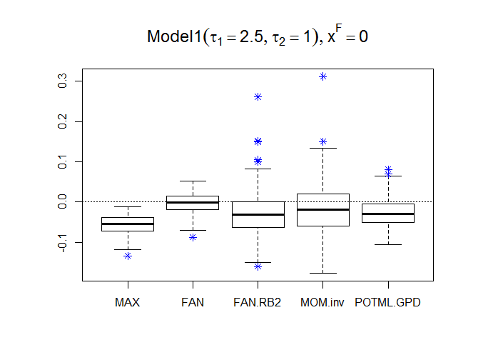
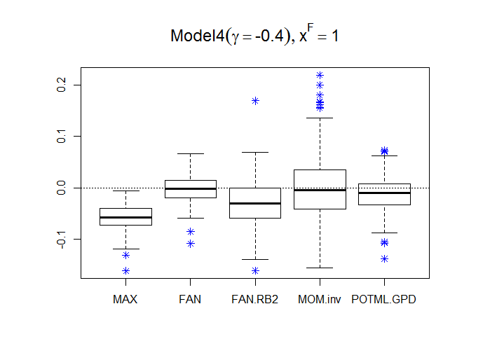
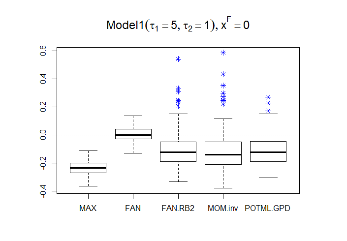
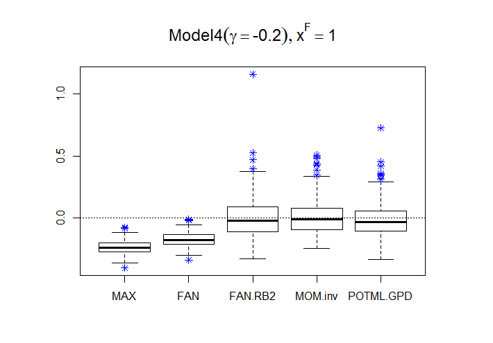
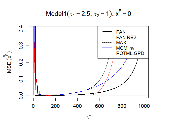
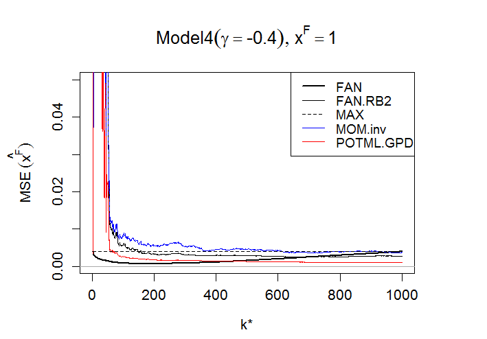
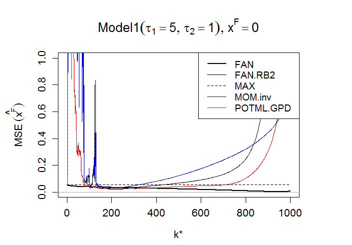
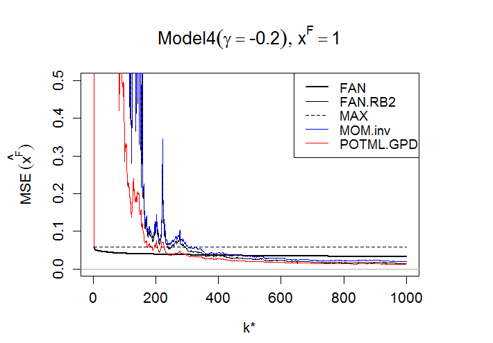
Figure 20: Boxplots of the errors $\varepsilon(j,k^{*}_{0}),\,\,j=1,\ldots,N=300$ (top) and Mean Squared Errors (MSE) plotted against $k^{*}$, $k^{*}\leq n$, (down) for MAX, FAN, FAN.RB2, MOM.inv and POTML.GPD endpoint estimators.

Some finite sample results for $\hat{x}^{F}_{RB2}$ are displayed in Figure 20. We have generate $N=300$ samples of size $n=1000$ from the parent Models 1 ($x^{F_{1}}=0$) and 4 ($x^{F_{4}}=1$). These models were introduced in the simulation study comprising section 4. Here, we have chosen to set the EVI at the values $-0.4$ and $-0.2$. The practical application in section 5 allows to foresee (cf. Figure 17) that by reducing the bias in the general endpoint estimator, we end up with a new estimator with larger variance. To this extent, we have furthermore anticipated a new estimator with very similar features to the designated MOM.inv and POTML.GPD endpoint estimators. Now, the simulation results seem to support our “guess”. The comparative box-plots in Figure 20 show a close resemblance of patterns within the group encompassing the three estimators FAN.RB2, MOM.inv and POTML.GPD, although there are situations in which the reduced bias version can serve as a good complement to the MOM.inv and POTML.GPD, particularly for the cases of anomalous behaviour of the likelihood surface, often encountered for the GPD. Figure 20 also illustrates the distinctive behavior of the general endpoint estimator, emphasizing lower MSE delivered by this estimator.

References

- Aarssen and de Haan, (1994) Aarssen, K. and de Haan, L. (1994). On the maximal life span of humans. Mathematical Population Studies, 4:259–281.
- Balkema and de Haan, (1974) Balkema, A. A. and de Haan, L. (1974). Residual life time at great age. Ann. Probab., 2:792–804.
- Bingham et al., (1987) Bingham, N. H., Goldie, C., and Teugels, J. L. (1987). Regular Variation. Encyclopedia of Mathematics and its Applications, vol. 27, Cambridge University Press.
- Cai et al., (2013) Cai, J. J., de Haan, L., and Zhou, C. (2013). Bias correction in extreme value statistics with index around zero. Extremes, 16:173–201.
- Castillo and Daoudi, (2009) Castillo, J. and Daoudi, J. (2009). Estimation of generalized Pareto distribution. Statistics & Probabiliy Letters, 79:684–688.
- Castillo and Serra, (2015) Castillo, J. and Serra, I. (2015). Likelihood inference for generalized Pareto distribution. Computational Statistics and Data Analysis, 83:116–128.
- Coles, (2011) Coles, S. (2011). Is there an upper limit to human longevity? AXA Global Forum for Longevity. Conference Proceedings from initial meetings, pages 96–103.
- Davison and Smith, (1990) Davison, A. and Smith, R. (1990). Models for exceedances over high thresholds. Journal of the Royal Statistical Society. Series B (Methodological), 52(3):393–442.
- de Haan, (1970) de Haan, L. (1970). On regular variation and its application to the weak convergence of sample extremes. Mathematisch Centrum Amsterdam.
- de Haan and Ferreira, (2006) de Haan, L. and Ferreira, A. (2006). Extreme Value Theory: An Introduction. Springer.
- de Haan et al., (2015) de Haan, L., Klein Tank, A., and Neves, C. (2015). On tail trend detection: modeling relative risk. Extremes, 18:141–178.
- Drees et al., (2004) Drees, H., Ferreira, A., and de Haan, L. (2004). On maximum likelihood estimation of the extreme value index. Ann. Appl. Probab., 14(3):1179–1201.
- Einmahl and Magnus, (2008) Einmahl, J. H. J. and Magnus, J. R. (2008). Records in athletics through extreme-value theory. JASA, 103:1382–1391.
- Ferreira et al., (2003) Ferreira, A., de Haan, L., and Peng, L. (2003). On optimising the estimation of high quantiles of a probability distribution. Statistics, 37(5):40–434.
- Fisher and Tippett, (1928) Fisher, R. A. and Tippett, L. H. C. (1928). Limiting forms of the frequency distribution of the largest and smallest member of a sample. Math. Proc. Cambridge Philos. Soc., 24:180–190.
- Fraga Alves et al., (2013) Fraga Alves, M. I., de Haan, L., and Neves, C. (2013). How far can Man go? In Torelli, N., Pesarin, F.,and Bar-Hen, A., editors, Advances in Theoretical and Applied Statistics. Springer, pages 185–195.
- Fraga Alves and Neves, (2014) Fraga Alves, M. I. and Neves, C. (2014). Estimation of the finite right endpoint in the Gumbel domain. Statist. Sinica, 24:1811–1835.
- Fries, (1980) Fries, J. (1980). Aging, natural death, and the compression of morbidity. New England Journal of Medicine, 303:130–135.
- Girard et al., (2011) Girard, S., Guillou, A., and Stupfler, G. (2011). Estimating an endpoint with high order moments. Test, 21:697–729.
- Girard et al., (2012) Girard, S., Guillou, A., and Stupfler, G. (2012). Estimating an endpoint with high order moments in the Weibull domain of attraction. Statist. Probab. Lett., 82:2136–2144.
- Gnedenko, (1943) Gnedenko, B. V. (1943). Sur la distribution limite du terme maximum d’une série aléatoire. Ann. of Math., 44:423–453.
- Grimshaw, (1993) Grimshaw, S. (1993). Computing maximum likelihood estimates for the generalized pareto distribution. Technometrics, 35(2):185–191.
- Hall, (1982) Hall, P. (1982). On estimating the endpoint of a distribution. Ann. Statist., 10:556–568.
- Hanayama, (2013) Hanayama, N. (2013). A discussion of the upper limit of human longevity based on study of data for oldest old survivors and deaths in japan. In Proceedings 59th ISI World Statistics Congress, pages 4518–4522.
- Hüsler and Peng, (2008) Hüsler, J. and Peng, L. (2008). Review of testing issues in extremes: in honor of Professor Laurens de Haan. Extremes, 11:99–111.
- Kaufmann and Reiss, (2007) Kaufmann, E. and Reiss, R. (2007). About the longevity of humans. Section 19.1 of Statistical Analysis of Extreme Values, pages 453–463.
- Li and Peng, (2010) Li, D. and Peng, L. (2010). Comparing extreme models when the sign of the extreme value index is known. Statistics & Probability Letters, 80(7-8):739–746.
- Neves and Fraga Alves, (2007) Neves, C. and Fraga Alves, M. I. (2007). Semi-parametric approach to Hasofer-Wang and Greenwood statistics in extremes. TEST, 16:297–313.
- Neves and Fraga Alves, (2008) Neves, C. and Fraga Alves, M. I. (2008). Testing extreme value conditions – an overview and recent approaches. REVSTAT - Statistical Journal, 6:83–100.
- Neves and Pereira, (2010) Neves, C. and Pereira, A. (2010). Detecting finiteness in the right endpoint of light-tailed distributions. Statistics and Probability Letters, 80:437–444.
- Neves et al., (2006) Neves, C., Picek, J., and Fraga Alves, M. (2006). Contribution of the maximum to the sum of excesses for testing max-domains of attraction. Journal of Statistical Planning and Inference, 136:1281–1301.
- (32) Olshansky, J., Carnes, B., and Cassel, C. (1990a). In search of methuselah: estimating the upper limits to human longevity. Science, 250:634––640.
- (33) Olshansky, S., Carnes, B., and Cassel, C. (1990b). In search of methuselah: estimating the upper limits to human longevity. Science, 250:634–640.
- Qi and Peng, (2009) Qi, Y. and Peng, L. (2009). Maximum likelihood estimation of extreme value index for irregular cases. Journal of Statistical Planning and Inference, 139:3361–3376.
- Smith, (1987) Smith, R. (1987). Estimating tails of probability distributions. The Annals of Statistics, 15(3):1174–1207.
- Stephenson and Tawn, (2013) Stephenson, A. and Tawn, J. (2013). Determining the best track performances of all time using a conceptual population model for athletics records. Journal of Quantitative Analysis in Sports, 9(1):67–76.
- Troen and Cristafalo, (2001) Troen, B. and Cristafalo, V. (2001). Principles and practice of geriatric surgery, chapter Cell and molecular aging, pages 8–23. Springer, New York.
- van der Vaart, (1998) van der Vaart, A. W. (1998). Asymptotic Statistics. Cambridge University Press.
- Vaupel, (2011) Vaupel, S. (2011). Longevity : What is it all about? AXA Global Forum for Longevity. Conference Proceedings from initial meetings, pages 2–9.
- Wang, (1995) Wang, J. (1995). Selection of the k largest order statistics for the domain of attraction of the Gumbel distribution. Journal of American Statistical Association, 90:1055–106.
- Wilmoth and Robine, (2003) Wilmoth, J. and Robine, J.-M. (2003). The world trend in maximum lifespan. Population and Development Review, 29:239–24.
- Zhou, (2010) Zhou, C. (2010). The extent of the maximum likelihood estimator for the extreme value index. Journal of Multivariate Analysis, 101(4):971 – 983.