Analytic continuation of Pasquier inversion representation of Khuri-Treiman equation

Abstract

The single integral form of Pasquier inversion representation of Khuri-Treiman (KT) equation presents great advantages for describing final state interaction of three-body decay or production processes. However, the original form of Pasquier inversion representation is only given in decay region and regions below. For the regions above, analytic continuation of original form is required. Because of non-trivial nature of analytic continuation procedure, it is the purpose of this work to obtain a well-defined Pasquier inversion representation of KT equation for all the energy range.

I Introduction

The theoretical framework for describing low energy hadronic three-body interaction has attracted significant attentions in the past, different approaches have been developed, such as field theory based Faddeev and Bethe-Salpeter type equations Faddeev:1960su ; Faddeev:1965su ; Taylor:1966zza ; Basdevant:1966zzb ; Gross:1982ny , and dispersion relation orientated Khuri-Treiman (KT) equation Khuri:1960zz ; Bronzan:1963xn . In processes, such as $\eta\rightarrow 3\pi$, three-body final state interaction has been reported to play a important role in explaining the discrepancy of Dalitz plot expansion parameters between experimental measurements and theoretical calculations Gasser:1984pr ; Kambor:1995yc ; Anisovich:1996tx ; Bijnens:2002qy ; Bijnens:2007pr ; Colangelo:2009db ; Zdrahal:2009cp ; Schneider:2010hs .

Among different methods, dispersion approach based KT equation shows some advantages because of it’s simplicity of formalism and analogue to naive isobar model approximation Goradia:1975ec ; Ascoli:1975mn . Since first proposed in Khuri:1960zz , KT equation has been further developed by many authors Bronzan:1963xn ; Aitchison:1965kt ; Aitchison:1965zz ; Aitchison:1966kt ; Pasquier:1968zz ; Pasquier:1969dt ; Guo:2014vya . Original form of KT equation is written in a form of double integrals dispersion equation, one integral comes from the dispersion integration and another is related to partial wave projection. By using Pasquier inversion technique Pasquier:1968zz ; Aitchison:1978pw ; Guo:2014vya , the order of two integrals can be exchanged, and it results in a single integral representation of KT equation that is more suitable for numerical computation Aitchison:1965kt ; Aitchison:1965zz ; Aitchison:1966kt ; Pasquier:1968zz ; Pasquier:1969dt ; Guo:2014vya . Unfortunately, original form of Pasquier inversion representation of KT equation is not well-defined for all the energy range, in fact, the original form is only given in the physical decay region and regions below. For other energy regions, analytic continuation of Pasquier inversion representation of KT equation has to be carried out deliberately to avoid singularities generated by contour integrations. As will be discussed in this work, the energy range above two-particle threshold is divided by a complex contour into three parts: decay, unphysical and scattering regions. Unphysical region is disconnected from decay and scattering regions, in this region, original form of KT equation has to be modified and an extra term is needed to keep solution of KT equation staying on physical sheet. Due to non-trivial procedure of analytic continuation, we describe some details of analytic continuation in this work, and present a well-defined form of Pasquier inversion representation of KT equation in all energy regions.

The paper is organized as follows. The original form of Pasquier inversion representation of KT equation is briefly introduced in Section II. The procedure of analytic continuation is described in Section III. The summary and conclusion are given in Section IV.

II Subenergy dispersion approach to three-body final state interaction

A general amplitude for a particle with spin-$J$ decays into three spinless particles, such as in $J/\psi$ decays Guo:2010gx ; Guo:2011aa , reads

$$\langle 123,\mbox{out}|J(\lambda),\mbox{in}\rangle=i(2\pi)^{4}\delta^{4}(\sum_{i=1,2,3}p_{i}-P)T_{\lambda},$$ (1)

where we denote the four momenta by $p_{i},P$ for i-th final state particle and initial decay particle, and $\lambda$ is the spin projection of the initial state along a fixed axis. Suppressing the isospin coupling among initial and final states, the amplitude $T_{\lambda}$ is given by,

$$T_{\lambda}(s,t,u)= \sum_{S,L,\mu}N_{SL\mu}D^{J*}_{\lambda,\mu}(r_{s})d^{S}_{\mu,0}(\theta_{s})a^{(s)}_{SL}(s)$$

$$+(s\rightarrow t)+(s\rightarrow u),$$ (2)

where the invariants are defined by $s=(p_{1}+p_{2})^{2}$, $t=(p_{2}+p_{3})^{2}$ and $u=(p_{3}+p_{1})^{2}$, and they are constrained by relation, $s+t+u=M^{2}+\sum_{i}m_{i}^{2}$ ($m_{i}$’s are final state particles masses and $M$ is mass of initial particle), and $N_{SL\mu}=\sqrt{(2S+1)(2L+1)}\langle S\mu;L0|J\mu\rangle$. The spin of pair $(12)$ is denoted by $S$, and the relative orbital angular momentum between $(12)$ and the third particle is given by $L$. $\theta_{s}$ is polar angle of particle-1 in pair $(12)$ rest frame. The rotation $r_{s}$, which is given by three Euler angles Guo:2010gx ; Guo:2011aa , rotates the standard configuration in $(12)3$ coupling scheme to the actual one. In the standard configuration of $(12)3$ coupling (rest frame of three-particle), third particle moves along negative $z$ axis while particle-1 and -2 move in the $xz$ plane. The amplitudes in $(23)1$ and $(31)2$ coupling schemes (denoted by $t$- and $u$-channel respectively) are defined in a similar way as in $(12)3$ coupling (denoted by $s$-channel). The dynamics of decay process are described by scalar functions $a^{(s,t,u)}_{SL}$, which only depend on subenergy of isobar pairs and possess only unitarity cut in subenergy by assumption Aitchison:1965zz ; Aitchison:1966kt ; Pasquier:1968zz .

For simplicity, in the following discussion, we consider the decay of a scalar particle, $J=0$, and truncate the partial waves to include only $S$-wave: $S=L=0$. Masses of final particles are assumed identical: $m_{1}=m_{2}=m_{3}=m$, and sub-channels are assumed symmetric: $a_{00}^{(s)}=a_{00}^{(t)}=a_{00}^{(u)}=a$. Thus, the decay amplitude is simply given by sum of three terms,

$$T(s,t,u)= a(s)+a(t)+a(u).$$ (3)

II.1 Khuri-Treiman equation and Pasquier inversion representation

The discontinuity of decay amplitude crossing unitarity cut in a subenergy, such as $s$, is given by

$$\triangle T(s,t,u)= \frac{T(s+i\epsilon,t,u)-T(s-i\epsilon,t,u)}{2i}$$

$$= \rho(s)f^{*}(s)\frac{1}{2}\int_{-1}^{1}dz_{s}T(s,t,u),$$ (4)

where $\rho(s)=\sqrt{1-4m^{2}/s}$, and $f(s)$ denotes $S$-wave two-body elastic scattering amplitude and is parametrized by phase shift of two-body scattering, $f=\left(e^{2i\delta}-1\right)/2i\rho$. $z_{s}=\cos\theta_{s}$ is given by $z_{s}=-(t-u)/\rho(s)k(s)$, where $k(s)=\sqrt{\left[s-(M-m)^{2}\right]\left[s-(M+m)^{2}\right]}$. A diagrammatic representation of discontinuity relations in Eq.(4) is shown in Fig.1.

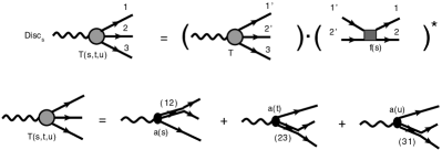
Figure 1: A diagrammatic representation of discontinuity relations in Eq.(4).

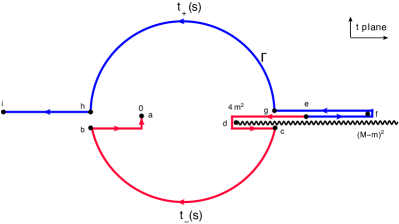
Figure 2: The path of $t_{\pm}(s)$ in $t$ complex plane as $s$ increased from $4m^{2}$ to $\infty$. The black waggle lines represent right hand cuts of $g(t)$ function. The points labeled by $a-i$ correspond to (a)$t_{-}(\infty)=0$, (b)$t_{-}\left((M+m)^{2}\right)=m(m-M)$, (c)$t_{-}\left((M-m)^{2}\right)=m(M+m)$, (d)$t_{-}\left((M^{2}-m^{2})/2\right)=4m^{2}$, (e)$t_{\pm}(4m^{2})=(M^{2}-m^{2})/2$, (f)$t_{+}\left(m(M+m)\right)=(M-m)^{2}$, (g)$t_{+}\left((M-m)^{2}\right)=m(M+m)$, (h)$t_{+}\left((M+m)^{2}\right)=m(m-M)$, and (i)$t_{+}(\infty)=-\infty$, respectively.

Figure 3: The path of $s_{\pm}(t)$ in $s$ complex plane for $t\in\left[-\infty,(M-m)^{2}\right]$. The arrows indicate the directions that invariants follow along the path of integrations. The black wiggle lines represent cuts attached to two branch points: $(M\pm m)^{2}$ in $s$ plane respectively. The points labeled by $a-f$ correspond to (a)$s_{-}(0)=-\infty$, (b)$s_{-}(4m^{2})=(M^{2}-m^{2})/2$, (c)$s_{-}\left((M^{2}-m^{2})/2\right)=4m^{2}$, (d)$s_{\pm}\left((M-m)^{2}\right)=m(m+M)$, (e)$s_{+}\left(m(M+m)\right)=(M-m)^{2}$, (f)$s_{+}(4m^{2})=(M^{2}-m^{2})/2$, (g)$s_{+}(0)=\infty$, (h)$s_{+}\left(m(m-M)\right)=(M+m)^{2}$, and (i)$s_{+}(-\infty)=\infty$, respectively.

By assumption, $a$’s possess only unitarity cuts, thus, $\triangle T(s,t,u)=\triangle a(s)$, and

$$\triangle a(s)=\rho(s)f^{*}(s)\left[a(s)+\frac{2}{\rho(s)k(s)}\int_{t_{-}(s)}^{t_{+}(s)}\!\!\!\!\!\!\!\!\ \!\!\!\!\!\!(\Gamma)\ dt\,a(t)\right],$$ (5)

where the factor $2$ in front of contour integral takes into account the contribution for $u$-channel. As discussed in Aitchison:1965zz ; Aitchison:1966kt ; Pasquier:1968zz ; Guo:2014vya , the angular projection in Eq.(4) is replaced by a contour integration in complex plane according to perturbation theory Bronzan:1963xn ; Bronzan:1964zz , contour $\Gamma$ is given in Fig.2. The boundaries of Dalitz plot, $t_{\pm}(s)$, are given by the solutions of $\phi(s,t_{\pm})=0$, where $\phi(s,t)=stu-m^{2}(M^{2}-m^{2})^{2}$, the analytic continuation of $t_{\pm}(s)$ in $s$ is specified by $\Gamma$, see Fig.2. The scalar function $a$ then is determined by subenergy dispersion relation,

$$a(s) =\frac{1}{\pi}\int_{4m^{2}}^{\infty}ds^{\prime}\frac{1}{s^{\prime}-s}\triangle a(s^{\prime}).$$ (6)

As discussed in Guo:2014vya , usually, it is useful to parameterize $a$ as a product of a known function and a reduced amplitude. For instance, we may choose parameterization, $a(s)=f(s)g(s)$, thus, the discontinuity relation for the reduced amplitude $g$ is given by Guo:2014vya ,

$$\triangle g(s)= -\theta(s_{L}-s)\frac{\mbox{Im}f(s)}{f^{*}(s)}g(s)$$

$$+\theta(s-4m^{2})\frac{2}{k(s)}\int_{t_{+}(s)}^{t_{-}(s)}\!\!\!\!\!\!\!\!\ \!\!\!\!\!\!(\Gamma)\ dt\,f(t)g(t),$$ (7)

where $s_{L}$ labels branch point of left hand cut in $f(s)$, and

$$g(s)=\frac{1}{\pi}\int_{-\infty}^{\infty}ds^{\prime}\frac{1}{s^{\prime}-s}\triangle g(s^{\prime}).$$ (8)

By using Pasquier inversion technique Aitchison:1965zz ; Aitchison:1966kt ; Pasquier:1968zz ; Guo:2014vya , also see Appendix A, we may obtain a single integral equation for $g$,

$$g(s)= -\frac{1}{\pi}\int_{-\infty}^{s_{L}}ds^{\prime}\frac{1}{s^{\prime}-s}\frac{\mbox{Im}f(s^{\prime})}{f^{*}(s^{\prime})}g(s^{\prime})+g_{R}(s),$$ (9)

where

$$g_{R}(s)=\frac{2}{\pi}\int_{-\infty}^{(M-m)^{2}}\!\!dt\,f(t)g(t)\left[\theta(t)\Delta(s,t)-\theta(-t)\Sigma(s,t)\right].$$ (10)

The kernel functions $\Delta$ and $\Sigma$ are given by

$$\Delta(s,t) =\int_{s_{-}(t)}^{s_{+}(t)}\!\!\!\!\!\!\!\!\ \!\!\!\!\!\!(C^{\prime})\ ds^{\prime}\frac{1}{U(s^{\prime})}\frac{1}{s^{\prime}-s},$$ (11)

$$\Sigma(s,t) =\int_{s_{+}(t)}^{s_{+}(\infty)}\!\!\!\!\!\!\!\!\!\!\!\!\!\!(C^{\prime})\ ds^{\prime}\frac{1}{U(s^{\prime})}\frac{1}{s^{\prime}-s},$$ (12)

where square root function $U(s)=\sqrt{\left[s-(M-m)^{2}\right]\left[s-(M+m)^{2}\right]}$ is defined in complex-$s$ plane, the phase convention for $U(s)$ is chosen by $U(s\pm i0)=(\mp,i,\pm)|U(s)|$ for $s\in([-\infty,(M-m)^{2}]$, $[(M-m)^{2},(M+m)^{2}],[(M+m)^{2},\infty])$ respectively. Thus, the square root $k(s)$ is given by the value of $U(s)$ right below two cuts attached to $(M\pm m)^{2}$, $k(s)=U(s-i0)$. The contour $C^{\prime}$ is given in Fig.3, and $s_{\pm}(t)$ are specified by solutions of $\phi(s_{\pm},t)=0$ and contour $C^{\prime}$.

The Pasquier inversion representation of $g(s)$ in Eq.(9-10) is initially defined in the range $s\in[-\infty,(M-m)^{2}]$ (on left and upper side of contour $C^{\prime}$). As will be made clear in section III, contour $C^{\prime}$ in kernel functions, $\Delta$ and $\Sigma$, is singular and divides $s$ plane into several isolated regions. Therefore, Eq.(9-10) can only hold for a complex $s$ that stays at the same side of contour $C^{\prime}$ and does not cross contour $C^{\prime}$. When $s$ is taken to cross contour $C^{\prime}$ to reach the region on the other side, for Pasquier inversion representation of KT equation to stay on physical sheet, $C^{\prime}$ has to be deformed and an extra piece is picked up as the consequence of deformation of contour. In follows, we present procedure of analytic continuation of Pasquier inversion representation of KT equation into $s\in[(M-m)^{2},\infty]$ regions.

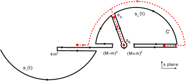
Figure 4: Analytic continuation of a function of type, $g_{R}(s)$ in Eq.(14), is followed by the motion of $s$ (red dashed curve). The physical sheet of $g_{R}(s)$ is defined in the upper half plane that is divided by contour $C^{\prime}$. Lower half plane can be reached by crossing $C^{\prime}$, when it does, a discontinuity has to be picked up to keep $g_{R}(s)$ on physical sheet.

III Analytic continuation of Pasquier inversion representation for $s\in[(M-m)^{2},\infty]$

As mentioned previously, $g(s)$ given by Eq.(9-10) is originally defined for $s\in[-\infty,(M-m)^{2}]$. The analytic continuation of first term on right hand side of Eq.(9) shows no difficulty, therefore we will only focus on the second term on right hand side of Eq.(9), $g_{R}(s)$, in following discussion. The $s$ dependence of $g(s)$ on second term, $g_{R}(s)$, is through kernel functions $\Delta$ and $\Sigma$, $\Delta$ and $\Sigma$ on physical sheet for $s\in[-\infty,(M-m)^{2}]$ are given by the value of $s$ running along the black wiggle line attached to $(M-m)^{2}$ in Fig.3. Therefore, the strategy of analytic continuation is that we start from here and then increase $s$ continuously until a singularity is encountered. Unfortunately for $g_{R}(s)$, contour $C^{\prime}$ presents a cut in complex-$s$ plane which stops us to naively use Eq.(9-10) in nearby region $s\in[(M-m)^{2},(M+m)^{2}]$. To illustrate this point, we first use the technique presented in Appendix A, and rewrite $g_{R}(s)$ to,

$$g_{R}(s)=\frac{2}{\pi}\int_{\Gamma^{\prime}}dt\,a(t)\int_{s_{\Gamma^{\prime}}(t)}^{\infty}\!\!\!\!\!\!\!\!\!\!(C^{\prime})\ ds^{\prime}\frac{1}{s^{\prime}-s}\frac{1}{U(s^{\prime})},$$ (13)

where contour $\Gamma^{\prime}$ is given in Fig.7, the location of $s_{\Gamma^{\prime}}(t)$ on $C^{\prime}$ is specified by the location of $t$ on $\Gamma^{\prime}$, see more details in Appendix A. Exchanging the order of two integrals leads to,

$$g_{R}(s)=\frac{2}{\pi}\int_{C^{\prime}}ds^{\prime}\frac{1}{s^{\prime}-s}\frac{1}{U(s^{\prime})}\int_{0}^{t_{C^{\prime}}(s^{\prime})}\!\!\!\!\!\!\!\!\!\!\!\!\!(\Gamma^{\prime})\ \ dt\,a(t),$$ (14)

where $t_{C^{\prime}}(s^{\prime})$ is inverse of $s_{\Gamma^{\prime}}(t)$, and Eq.(14) is similar to Eq.(23) but with contours $C^{\prime}$ and $\Gamma^{\prime}$ instead. Now, we can clearly see the cut structure on $s$ generated by contour $C^{\prime}$ in Eq.(14). As $s$ is moved from left hand side of $C^{\prime}$ in region $s\in[-\infty,(M-m)^{2}]$ to reach $s\in[(M-m)^{2},(M+m)^{2}]$ region by crossing contour $C^{\prime}$ (motion of $s$ is demonstrated in Fig.4 by red dashed curve), $C^{\prime}$ has to be deformed to keep $g_{R}(s)$ on physical sheet. For a example, at a point $s_{A}$ in Fig.4, which sits right next to the inside circle of $C^{\prime}$ in complex plane, then, $g_{R}(s_{A})$ on physical sheet is given by,

$$g_{R}(s_{A})= \frac{2}{\pi}\int_{C^{\prime}}ds^{\prime}\frac{1}{s^{\prime}-s_{A}}\frac{1}{U(s^{\prime})}\int_{0}^{t_{C^{\prime}}(s^{\prime})}\!\!\!\!\!\!\!\!\!\!\!\!\!(\Gamma^{\prime})\ \ dt\,a(t)$$

$$+ \frac{4i}{U(s_{A})}\int_{0}^{t_{C^{\prime}}(s_{A})}\!\!\!\!\!\!\!\!\!\!\!\!\!\!\!(\Gamma^{\prime})\ \ dt\,a(t).$$ (15)

Next, $s$ is moved away from $s_{A}$ to a point on real axis in region $s\in[(M-m)^{2},(M+m)^{2}]$, such as $s_{B}$ in Fig.4, thus $C^{\prime}$ is further deformed to follow the motion of $s$. When $s$ reach real axis, $C^{\prime}$ in second term on the right hand side of Eq.(15) collapse onto real axis and $\Gamma^{\prime}$ opens up accordingly into $\Gamma$, thus, for $s\in[(M-m)^{2},(M+m)^{2}]$ on the real axis, we obtain,

$$g_{R}(s)= \frac{2}{\pi}\int_{-\infty}^{(M-m)^{2}}\!\!dt\,a(t)\left[\theta(t)\Delta(s,t)-\theta(-t)\Sigma(s,t)\right]$$

$$+ \frac{4i}{U(s)}\int_{0}^{t_{+}(s)}\!\!\!\!\!\!\!\!\!\!\!(\Gamma)\ dt\,a(t),$$

$$\quad\quad\quad\ \ \mbox{for}\ \ s\in[(M-m)^{2},(M+m)^{2}].$$ (16)

At last, the analytic continuation of $g_{R}(s)$ from $s\in[-\infty,(M-m)^{2}]$ to region $s\in[(M+m)^{2},\infty]$, where $s$ runs along black wiggle line attached to $(M+m)^{2}$ in Fig.3, does not encounter any singularities and so it does not require the deformation of contour $C^{\prime}$, see the motion of red dashed curve in Fig.4, therefore $g_{R}(s)$ in Eq.(10) remains unchanged for $s\in[(M+m)^{2},\infty]$.

On the other hand, we may also perform the analytic continuation of Pasquier inversion representation of KT equation through a triangle diagram. Using Eq.(6), we first rewrite Eq.(9-10) to

$$g(s)= -\frac{1}{\pi}\int_{-\infty}^{s_{L}}ds^{\prime}\frac{1}{s^{\prime}-s}\frac{\mbox{Im}f(s^{\prime})}{f^{*}(s^{\prime})}g(s^{\prime})$$

$$+\frac{2}{\pi}\int_{4m^{2}}^{\infty}dt^{\prime}\triangle a(t^{\prime})\mathcal{G}(s,t^{\prime}),$$

$$\quad\quad\quad\quad\quad\quad\quad\quad\mbox{for}\ \ s<(M-m)^{2},$$ (17)

where $\mathcal{G}$ is given by,

$$\mathcal{G}(s,t^{\prime})= \frac{1}{\pi}\int_{-\infty}^{(M-m)^{2}}\!\!dt\frac{1}{t^{\prime}-t}\left[\theta(t)\Delta(s,t)-\theta(-t)\Sigma(s,t)\right],$$

$$\quad\quad\quad\quad\mbox{for}\ \ t^{\prime}>4m^{2},s<(M-m)^{2}.$$ (18)

$\mathcal{G}$ is identified as the Pasquier inversion representation of a triangle diagram in region $t^{\prime}>4m^{2},s<(M-m)^{2}$. The analytic continuation of $\mathcal{G}$ in different representations is presented in Appendix B, the Pasquier inversion representation of $\mathcal{G}$ for $(s,t^{\prime})\in[-\infty,\infty]$ is given by Eq.(B.2),

$$\mathcal{G}(s,t^{\prime}) =\frac{1}{\pi}\int_{-\infty}^{(M-m)^{2}}dt\frac{1}{t^{\prime}-t}\left[\theta(t)\Delta(s,t)-\theta(-t)\Sigma(s,t)\right]$$

$$+2i\theta\left(s-(M-m)^{2}\right)\theta\left((M+m)^{2}-s\right)$$

$$\quad\times\left[\frac{1}{U(s)}\int_{0}^{t_{+}(s)}\!\!\!\!\!\!\!\!\!\!\!(\Gamma)\ \frac{dt}{t^{\prime}-t}+\theta(t^{\prime})\theta(4m^{2}-t^{\prime})\frac{2\pi i}{U(s)}\right],$$

$$\quad\quad\quad\quad\quad\quad\quad\quad\quad\quad\quad\mbox{for}\ \ (s,t^{\prime})\in[-\infty,\infty].$$

The $s$ dependence of $g(s)$ in second term in Eq.(III) is all through triangle diagram $\mathcal{G}$, thus, analytic continuation of $\mathcal{G}$ completes the analytic continuation of Pasquier inversion representation of $g(s)$. Plugging Eq.(B.2) back into Eq.(III), we once again obtain the Pasquier inversion representation of $g(s)$ for $s\in[-\infty,\infty]$,

$$g(s) =-\frac{1}{\pi}\int_{-\infty}^{s_{L}}ds^{\prime}\frac{1}{s^{\prime}-s}\frac{\mbox{Im}f(s^{\prime})}{f^{*}(s^{\prime})}g(s^{\prime})$$

$$+\frac{2}{\pi}\int_{-\infty}^{(M-m)^{2}}\!\!dtf(t)g(t)\left[\theta(t)\Delta(s,t)-\theta(-t)\Sigma(s,t)\right]$$

$$+4i\theta\left(s-(M-m)^{2}\right)\theta\left((M+m)^{2}-s\right)$$

$$\quad\quad\quad\quad\quad\quad\quad\quad\quad\times\frac{1}{U(s)}\int_{0}^{t_{+}(s)}\!\!\!\!\!\!\!\!\!\!\!(\Gamma)\ dtf(t)g(t),$$

$$\quad\quad\quad\quad\quad\quad\quad\quad\quad\mbox{for}\ \ s\in[-\infty,\infty].$$ (19)

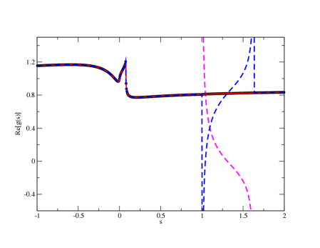
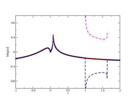
Figure 5: The real (top plot) and imaginary (bottom plot) parts of $g(s)$ by solving both dispersion representation Eq.(II.1-8) (black circles) and Pasquier inversion representation Eq.(III) (solid red curves). Blue dashed curves are the solution of $g(s)$ from Eq.(9-10) without proper analytic continuation, purple dashed curves represent contribution from extra term picked up by analytic continuation in Eq.(III), $4i/U(s)\int_{0}^{t_{+}(s)}(\Gamma)dta(t)$. The input model of $f(s)$ is taken from Eq.(28) in Guo:2014vya , with fixed parameters: $\alpha=0.1$, $\beta=0.2$, $m_{R}=0.8$ GeV, $m=0.14$ GeV and $M=1.14$ GeV. The left hand cut of $f(s)$ is placed at $s_{L}=0$ and $g(s)$ is normalized to $g(0)=1$.

The analytic continuation of Pasquier inversion representation of $g(s)$ given by Eq.(III) is tested numerically by using a toy model for $f(s)$, model of $f(s)$ is taken from Guo:2014vya . The comparison of $g(s)$’s by solving Pasquier inversion representation Eq.(III) and dispersion representation Eq.(II.1-8) is shown in Fig.5. We also shown the results by solving Eq.(9-10) without proper analytic continuation compared to the contribution of extra term that is picked up by analytic continuation, $4i/U(s)\int_{0}^{t_{+}(s)}(\Gamma)dta(t)$. As demonstrated in Fig.5, solution of analytic continuation of Pasquier inversion representation of $g(s)$ is consistent with dispersion representation of $g(s)$. Solution of Pasquier inversion representation of $g(s)$ without proper analytic continuation jumps in unphysical region $s\in[(M-m)^{2},(M+m)^{2}]$, extra term, $4i/U(s)\int_{0}^{t_{+}(s)}(\Gamma)dta(t)$, is needed to keep $g(s)$ continuous and staying on physical sheet.

At last, similarly, if we parametrize $a(s)=G(s)/D(s)$ Guo:2014vya , where $D(s)=N(s)/f(s)$ contains only unitarity cut of scattering amplitude and all other cuts are absorbed into function $N(s)$ Chew:1960iv ; Frye:1963zz , thus we obtain,

$$G(s)= \frac{2}{\pi}\int_{-\infty}^{(M-m)^{2}}\!\!dt\frac{G(t)}{D(t)}\left[\theta(t)\Delta_{G}(s,t)-\theta(-t)\Sigma_{G}(s,t)\right]$$

$$+ 4i\theta\left(s-(M-m)^{2}\right)\theta\left((M+m)^{2}-s\right)$$

$$\quad\quad\quad\quad\quad\quad\quad\quad\times\frac{N(s)}{U(s)}\int_{0}^{t_{+}(s)}\!\!\!\!\!\!\!\!\!\!\!(\Gamma)\ dt\frac{G(t)}{D(t)},$$

$$\quad\quad\quad\quad\quad\quad\quad\quad\mbox{for}\ \ s\in[-\infty,\infty],$$ (20)

where the kernel functions $\Delta_{G}$ and $\Sigma_{G}$ are given by Eq.(29) and (29) respectively.

IV Summary

We presented the analytic continuation procedure of Pasquier inversion representation of KT equation, and a well-defined Pasquier inversion representation of KT equation for an arbitrary $s$ on real axis is given by Eq.(III) and Eq.(20).

Comparing the Pasquier inversion representation of KT equation in Eq.(III) to dispersion representation of KT equation in Eq.(II.1-8), as has been also discussed in Guo:2014vya , the single integral form of Pasquier inversion representation in Eq.(III) indeed present a significant advantage on numerical computation in regions $s\in[-\infty,(M-m)^{2}]$ and $s\in[(M-m)^{2},\infty]$. However, in unphysical region $s\in[(M-m)^{2},(M+m)^{2}]$, dispersion representation in Eq.(II.1-8) requires no extra efforts, but analytic continuation of Pasquier inversion representation becomes non-trivial and need an extra term to keep solution, $g(s)$, staying on physical sheet. At last, we solved Pasquier inversion representation of KT equation in Eq.(III) numerically by using a toy model of $f(s)$, solutions with and without proper analytic continuation compared to the solution of dispersion representation are illustrated in Fig.5.

V ACKNOWLEDGMENTS

We thank Adam P. Szczepaniak for many fruitful discussion. We acknowledge supports in part by the U.S. Department of Energy under Grant No. DE-FG0287ER40365 and the Indiana University Collaborative Research Grant. We also acknowledge support from U.S. Department of Energy contract DE-AC05-06OR23177, under which Jefferson Science Associates, LLC, manages and operates Jefferson Laboratory.

Appendix A Pasquier inversion technique

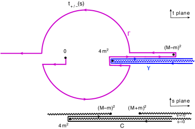
Figure 6: The path of $t_{\pm}(s)$ (solid purple curves), contour $C$ (solid black lines) and $\gamma$ (solid blue lines). The arrows indicate the directions that invariants follow in double integrations, Eq.(21) and (24). The blue wiggle line represents the unitarity cut in $t$ plane, and black wiggle lines represent the cuts in $s$ plane.

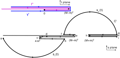
Figure 7: The contour $\Gamma^{\prime}$ (solid purple lines), $C^{\prime}$ (solid black curves) and $\gamma^{\prime}$ (solid blue lines) in Eq.(27). The arrows indicate the directions that invariants follow along the path of integrations. The purple and black wiggle lines represent unitarity cut in $s$ plane and cuts attached to two branch points: $(M\pm m)^{2}$ in $s$ plane respectively.

For completeness, we present the Pasquier inversion technique Pasquier:1968zz ; Aitchison:1978pw in this section. Considering a double integrals equation of type,

$$I(s)=\int_{4m^{2}}^{\infty}ds^{\prime}\frac{1}{s^{\prime}-s}\frac{N(s^{\prime})}{k(s^{\prime})}\int_{t_{-}(s^{\prime})}^{t_{+}(s^{\prime})}\!\!\!\!\!\!\!\!\!\!\!(\Gamma)\ dt\,a(t),$$ (21)

where contour $\Gamma$ followed by $t$ integration is defined to avoid unitarity cut in $a$, see Fig.2, and the integration path of $s^{\prime}$ is defined on the real axis, the physical value of $I(s)$ is given by $s$ running above real axis.

As described in Pasquier:1968zz ; Aitchison:1978pw , we first split $t$ integral into two pieces and rewrite the double integrals in Eq.(21) to

$$I(s)=\int_{4m^{2}}^{\infty}ds^{\prime}\frac{1}{s^{\prime}-s}\frac{N(s^{\prime})}{k(s^{\prime})}\left[\int_{0}^{t_{+}(s^{\prime})}\!\!\!\!\!\!\!\!\!\!\!\!(\Gamma)\ -\int_{0}^{t_{-}(s^{\prime})}\!\!\!\!\!\!\!\!\!\!\!\!(\Gamma)\ \ \right]dt\,a(t).$$ (22)

Then, for first term in bracket in Eq.(22), the path of $s^{\prime}$ integration is shifted to above real axis, and for second term in bracket in Eq.(22), the path of $s^{\prime}$ integration is shifted to below real axis. Note that kinematic function $k(s^{\prime})$ as a function of $s^{\prime}$ has two branch points: $(M\pm m)^{2}$. Two cuts may be attached to these two points, one runs from $-\infty$ up to $(M-m)^{2}$ and another runs from $(M+m)^{2}$ up to $\infty$, see black wiggle lines in Fig.6. As we have mentioned before, $U$ is defined as the continuation of $k(s^{\prime})$ for a complex argument, the physical value of $k(s^{\prime})$ is given by taking the branch of $U(s^{\prime})$ below two cuts attached to $(M\pm m)^{2}$, $k(s^{\prime})=U(s^{\prime}-i0)$. These two kinematic cuts are placed above both real axis and shifted $s^{\prime}$ integration paths described previously, see Fig.6, therefore, operation of shifting $s^{\prime}$ integration paths is valid and $s^{\prime}$ integration paths do not interfere with cuts in $U$. Thus, we can safely rewrite the double integrals in Eq.(22) to,

$$I(s)=\int_{C}ds^{\prime}\frac{1}{s^{\prime}-s}\frac{N(s^{\prime})}{U(s^{\prime})}\int_{0}^{t_{C}(s^{\prime})}\!\!\!\!\!\!\!\!\!\!\!\!(\Gamma)\ \ dt\,a(t),$$ (23)

where the path $C$ of $s^{\prime}$ integral is shown in Fig.6, whether $t_{C}(s^{\prime})$ is $t_{+}(s^{\prime})$ or $t_{-}(s^{\prime})$ depends on which portion of path $C$ the invariant $s^{\prime}$ is on. $t_{+}(t_{-})$ is assigned to $s^{\prime}$ on the portion of $C$ above(below) real axis. In Eq.(23), the physical value of $I(s)$ is given by $s$ running above contour $C$. Next, we exchange the order of two integrals, so that Eq.(23) becomes,

$$I(s)=\int_{\Gamma}dt\,a(t)\left[\int_{s_{\Gamma}(t)}^{\infty}\!\!\!\!\!\!\!\!\!(C)\ ds^{\prime}\frac{1}{s^{\prime}-s}\frac{N(s^{\prime})}{U(s^{\prime})}\right],$$ (24)

where $t$ integration on contour $\Gamma$ runs from $0$ to $-\infty$ by looping around threshold $(M-m)^{2}$, see Fig.6, and $s^{\prime}$ integration runs from $s_{\Gamma}(t)$ up to $\infty$ along path $C$, $s_{\Gamma}(t)$ is given by the inverse of $t_{C}(s^{\prime})$. By assumption, $a$ has only unitarity cut, using Cauchy’s theorem, we can write a equation,

$$a(t)=\frac{1}{2\pi i}\int_{\gamma}dt^{\prime}\frac{a(t^{\prime})}{t^{\prime}-t},$$ (25)

where contour $\gamma$ loops around the unitarity cut but avoiding interference with $\Gamma$, see in Fig.6, the convergence of integration has been assumed valid so that the circle of contour $\gamma$ at infinity can be dropped. Thus, we obtain,

$$I(s)= \frac{1}{2\pi i}\int_{\gamma}dt^{\prime}\,a(t^{\prime})\left[\int_{\Gamma}\frac{dt}{t^{\prime}-t}\int_{s_{\Gamma}(t)}^{\infty}\!\!\!\!\!\!\!\!(C)\ ds^{\prime}\frac{1}{s^{\prime}-s}\frac{N(s^{\prime})}{U(s^{\prime})}\right].$$ (26)

When $N$ function is replaced by a constant, the function in bracket in Eq.(26) may be associated to a triangle diagram, see Appendix B. The next step is to deform the contour $\gamma$ onto real axis toward $-\infty$ but avoid both unitarity cut in $a$ and the singularities from the expression in bracket in Eq.(26). By construction of $\Gamma$, unitarity cut of $a$ sits along the blue wiggle line in Fig.6, and $a(t)$ for $t$ running above unitarity cut is defined physical. Therefore, as long as deformation of $\gamma$ and $\Gamma$ toward negative real axis does not interfere with unitarity cut of $a$, $a$ remains on physical sheet all the time. Singularities of the function in bracket in Eq.(26) have been extensively studied by authors in Aitchison:1965zz ; Pasquier:1968zz ; Aitchison:1964ta ; Aitchison:1964nc ; Kacser:1966ta from perturbation theory perspective, they are branch points at $t=0,4m^{2}$ and $(M-m)^{2}$. One may attach branch cuts to those branch points running toward negative real axis Aitchison:1965zz ; Pasquier:1968zz ; Aitchison:1964ta ; Aitchison:1964nc ; Kacser:1966ta , therefore, the contour $\gamma^{\prime}$ may be chosen to loop around the threshold $(M-m)^{2}$ toward negative real axis. The deformation of contour $\gamma$ also drags the contour $\Gamma$ going with it back onto real axis, the correspondent contour $C$ must then be opened up accordingly. Simultaneously, in order for $I(s)$ staying on physical sheet, some $s$ are also dragged by the deformation of $C$ into complex plane, and physical value of $I(s)$ is now given by a $s$ that sits on the same side of $C$ when it opens up into complex plane. The only $t^{\prime}$-dependent singularities come from factor $1/(t^{\prime}-t)$ in bracket in Eq.(26), so that, when contour $\gamma$ is collapsed onto real axis, the discontinuity of this factor $1/(t^{\prime}-t)$ along the cut from $-\infty$ to $(M-m)^{2}$ is picked up. Equivalently, we may replace $\int_{\gamma}dt^{\prime}/(t^{\prime}-t)$ by $2\pi i\int_{-\infty}^{(M-m)^{2}}dt^{\prime}\delta(t^{\prime}-t)$ in Eq.(26). Therefore, Eq.(26) becomes,

$$I(s)= \int_{\Gamma^{\prime}}dt\,a(t)\left[\int_{s_{\Gamma^{\prime}}(t)}^{\infty}\!\!\!\!\!\!\!\!\!\!(C^{\prime})\ ds^{\prime}\frac{1}{s^{\prime}-s}\frac{N(s^{\prime})}{U(s^{\prime})}\right].$$ (27)

The contours $C^{\prime}$ and $\Gamma^{\prime}$ have to be chosen to avoid the singularities in integrands. Examining Eq.(27), we note that integrands of contour integration over invariant $s^{\prime}$ are only the product of $1/(s^{\prime}-s)$, kinematic function $U$ and left hand cut function $N$. As we have mentioned early, kinematic function $U$ as a function of $s^{\prime}$ has two branch points: $(M\pm m)^{2}$, two cuts are attached to these two points, one runs toward $-\infty$ and another runs toward $\infty$ respectively, see black wiggle lines in Fig.7. Therefore, the contour $C^{\prime}$ may be chosen to avoid two cuts attached to $(M\pm m)^{2}$, as plotted in Fig.7. With this choice, the function in bracket in Eq.(27) may be associated to the discontinuities of triangle diagram defined in Eq.(26) along the cut attached to branch point $(M-m)^{2}$ in $t$ plane. Similar to $\gamma^{\prime}$, the contour $\Gamma^{\prime}$ also loops around the point $(M-m)^{2}$ and is placed above unitarity cut in $a$. Whether $s_{\Gamma^{\prime}}(t)$ is $s_{+}(t)$ or $s_{-}(t)$ depends on whether $t$ is above or below the cut attached to $(M-m)^{2}$ in $t$ plane respectively, see Fig.7.

As mentioned early, the physical value of $I(s)$ was chosen by $s$ running above contour $C$ in Eq.(23), when $C$ is deformed to $C^{\prime}$, see Fig.6 and Fig.7. In order for $I(s)$ to stay on physical sheet, $s$ is not allowed to cross contour, as a result, some $s$ are forced to follow the deformation of contour into complex plane. Specifically, (1) for $s\in[-\infty,(M-m)^{2}]$, the physical value of $I(s)$ is given by $s$ running along the black wiggle line attached to $(M-m)^{2}$, (2) for $s\in[(M-m)^{2},\infty]$, now physical $I(s)$ is trapped into the value of $s$ running along balck wiggle line attached to $(M+m)^{2}$ between sections $g-h$ and $h-i$ on $C^{\prime}$, and (3) the form of $I(s)$ in Eq.(27) for $s\in[(M-m)^{2},(M+m)^{2}]$ on real axis is no longer on the physical sheet, physical $I(s)$ now is given by a complex $s$ running on the upper side of arc $f-g$ on $C^{\prime}$. To reach physical $I(s)$ for $s\in[(M-m)^{2},(M+m)^{2}]$ on real axis, the analytic continuation is required, the procedure is described in section III.

At last, by splitting $s^{\prime}$ integration path, $\int_{\Gamma^{\prime}}=\left[\int_{0_{-}}^{(M-m)^{2}_{-}}-\int^{(M-m)^{2}_{+}}_{0_{+}}\right]+\int_{0_{+}}^{-\infty_{+}}$ in Eq.(27) (subscript $+/-$ of integration limits denotes the path of integration lying above or below the cut attached to branch point $(M-m)^{2}$ in $t$ plane, see Fig.7), we obtain,

$$I(s)=\int_{-\infty}^{(M-m)^{2}}\!\!\!\!dt\,a(t)\left[\theta(t)\Delta_{G}(s,t)-\theta(-t)\Sigma_{G}(s,t)\right],$$ (28)

where

$$\Delta_{G}(s,t) =\int_{s_{-}(t)}^{s_{+}(t)}\!\!\!\!\!\!\!\!\ \!\!\!\!\!\!(C^{\prime})\ ds^{\prime}\frac{1}{s^{\prime}-s}\frac{N(s^{\prime})}{U(s^{\prime})},$$ (29)

$$\Sigma_{G}(s,t) =\int_{s_{+}(t)}^{\infty}\!\!\!\!\!\!\!\!\ \!\!\!(C^{\prime})\ ds^{\prime}\frac{1}{s^{\prime}-s}\frac{N(s^{\prime})}{U(s^{\prime})}.$$ (30)

For $s$ on real axis, value of $\Delta_{G}$ and $\Sigma_{G}$ on physical sheet is only defined in regions, $[-\infty,(M-m)^{2}]$ and $[(M+m)^{2},\infty]$. For $s\in[(M-m)^{2},(M+m)^{2}]$, $\Delta_{G}$ and $\Sigma_{G}$ given by Eq.(29-30) without proper analytic continuation are on unphysical sheet. For the case $N(s)=1$, the corresponding kernels are denoted as $\Delta$ and $\Sigma$.

Kernel functions $\Delta$ and $\Sigma$ can be expressed in terms of elementary functions. For real $s$ and $t$, the value of $\Delta$ and $\Sigma$ given below by Eq.(31-34) are simply corresponding to the limit $s+i0$ and $t+i0$, and again, Eq.(32) and (34) are defined on unphysical sheet,

$$\Delta(s,t) =\frac{1}{U(s)}\ln|\frac{R(s,t)+U(s)U(t)}{R(s,t)-U(s)U(t)}|-\theta\left(\phi(s,t)\right)\frac{i\pi}{U(s)},$$

$$\mbox{for}\ \ t\in[0,(M-m)^{2}],$$

$$\quad\ \ s\in[-\infty,(M-m)^{2}]\&[(M+m)^{2},\infty],$$ (31)

and

$$\Delta(s,t)=\frac{1}{U(s)}\ln\frac{R(s,t)+U(s)U(t)}{R(s,t)-U(s)U(t)}$$

$$\quad\quad\quad\quad-\theta\left(m(m+M)-t\right)\theta\left(s_{R}(t)-s\right)\frac{2i\pi}{U(s)},$$

$$\mbox{for}\ \ t\in[0,(M-m)^{2}],s\in[(M-m)^{2},(M+m)^{2}],$$ (32)

where $R(s,t)=-M^{4}+(s-m^{2})(t-m^{2})+M^{2}(s+t)$ and $s_{R}(t)$ is given by the solution of $R(s_{R},t)=0$.

$$\Sigma(s,t)=\frac{1}{U(s)}\ln|L(s,t)|-\theta\left(s-s_{+}(t)\right)\frac{i\pi}{U(s)},$$

$$\mbox{for}\ \ t<0,s\in[-\infty,(M-m)^{2}]\&[(M+m)^{2},\infty],$$ (33)

and

$$\Sigma(s,t)=\frac{1}{U(s)}\ln L(s,t)-\theta\left(\mbox{Im}L(s,t)\right)\frac{2i\pi}{U(s)},$$

$$\quad\quad\quad\mbox{for}\ \ t<0,s\in[(M-m)^{2},(M+m)^{2}],$$ (34)

where

$$L(s,t)$$

$$=\frac{\left[s_{+}(t)-s\right]\left[s-M^{2}-m^{2}+U(s)\right]}{\left[s_{+}(t)-s\right](s-M^{2}-m^{2})+U^{2}(s)-U(s)U(s_{+}(t))}.$$

Figure 8: A triangle diagram with a fixed internal mass $\sqrt{t}$ in $(23)$ sub-channel.

Appendix B Different representations of a triangle diagram

From perturbation theory, the Feynman parametrization of a triangle diagram in Fig.8 is given by Bronzan:1963xn ,

$$\mathcal{G}(s,t)=\frac{1}{\pi}\int_{0}^{1}d\alpha_{1}d\alpha_{2}d\alpha_{3}$$

$$\times\frac{\delta(1-\alpha_{1}-\alpha_{2}-\alpha_{3})}{\alpha_{1}t+(1-\alpha_{1}-\alpha_{1}\alpha_{2})m^{2}-\alpha_{3}(\alpha_{1}M^{2}+\alpha_{2}s)-i\epsilon},$$ (35)

where $t$ denotes the invariant mass square of pair $(23)$ propagator. The analytic continuation of Feynman parametrization representation of $\mathcal{G}$ as a function of complex arguments $(s,t)$ is carried out by $i\epsilon$ prescription Bronzan:1963xn .

In follows, we present the analytic continuation of both dispersion representation and Pasquier inversion representation of $\mathcal{G}$, the strategy is that we start at a region where a representation of $\mathcal{G}$ is defined on physical sheet and consistent with perturbation theory result Eq.(B), then, $\mathcal{G}$ is continued to other regions by using perturbation theory result Eq.(B) as a reference.

(1) The dispersion representation of a triangle diagram for $t>4m^{2}$ has been discussed in Bronzan:1963xn ,

$$\mathcal{G}(s,t)= \frac{1}{\pi}\int_{4m^{2}}^{\infty}ds^{\prime}\frac{1}{s^{\prime}-s}\left[\frac{1}{k(s^{\prime})}\int_{t_{-}(s^{\prime})}^{t_{+}(s^{\prime})}\!\!\!\!\!\!\!\!\!\!\!\!(\Gamma)\ \ dt^{\prime}\frac{1}{t-t^{\prime}}\right],$$

$$\quad\quad\quad\quad\quad\quad\quad\quad\mbox{for}\ \ t>4m^{2}.$$ (36)

(2) The Pasquier inversion representation of a triangle diagram for $s<(M-m)^{2}$ is given by Guo:2014vya ,

$$\mathcal{G}(s,t)= \frac{1}{\pi}\int_{-\infty}^{(M-m)^{2}}\!\!\frac{dt^{\prime}}{t-t^{\prime}}\left[\theta(t^{\prime})\Delta(s,t^{\prime})-\theta(-t^{\prime})\Sigma(s,t^{\prime})\right],$$

$$\quad\quad\quad\quad\quad\quad\quad\quad\mbox{for}\ \ s<(M-m)^{2}.$$ (37)

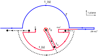
Figure 9: Analytic continuation of a function in $t$ of type, $\mathcal{G}(s,t)$ in Eq.(38), is followed by the motion of $t$ (black dashed curve). The physical sheet of $\mathcal{G}(s,t)$ in $t$ is defined in outside space of $\Gamma$. $t\in[0,4m^{2}]$ inside of $\Gamma$ region can be reached by crossing $\Gamma$, then a discontinuity has to be picked up to keep $\mathcal{G}(s,t)$ on physical sheet.

B.1 Analytic continuation of dispersion representation of triangle diagram

We first perform analytic continuation of dispersion representation of $\mathcal{G}$ in Eq.(B). Note that the overlapping region for both dispersion representation and Pasquier inversion representation of $\mathcal{G}$ on physical sheet is $t\in[4m^{2},\infty]$ and $s\in[-\infty,(M-m)^{2}]$. As described in Appendix A, exchanging order of double integrals encounters no extra singularities in this region, so, we start from here and rewrite Eq.(B) to, see Eq.(21-24),

$$\mathcal{G}(s,t)= \frac{1}{\pi}\int_{\Gamma}dt^{\prime}\frac{1}{t-t^{\prime}}\left[\int_{s_{\Gamma}(t^{\prime})}^{\infty}\!\!\!\!\!\!\!\!\!\!(C)\ ds^{\prime}\frac{1}{s^{\prime}-s}\frac{N(s^{\prime})}{U(s^{\prime})}\right],$$

$$\quad\quad\quad\quad\mbox{for}\ \ t>4m^{2},s<(M-m)^{2}.$$ (38)

The cut in $t$ generated by contour $\Gamma$ is now explicitly given by $\int_{\Gamma}dt^{\prime}/(t-t^{\prime})$, we start with $t$ running along the black wiggle line in Fig.2, where $\mathcal{G}$ is defined on physical sheet. As long as the motion of $t$ in complex plane does not interfere with the contour $\Gamma$, $\mathcal{G}$ remains on physical sheet, thus, Eq.(B) still holds for $t<0$, see the motion of $t$ represented by black dashed curve in Fig.9. However, when $t$ is moved to cross contour $\Gamma$, the contour $\Gamma$ has to be deformed to keep $\mathcal{G}$ on physical sheet. To reach region $t\in[0,4m^{2}]$, we can first move $t$ to $t_{A}$ which is a point sits right inside circle of $\Gamma$, see Fig.9. Thus, the deformation of $\Gamma$ leads to

$$\mathcal{G}(s,t_{A})= \frac{1}{\pi}\int_{\Gamma}dt^{\prime}\frac{1}{t_{A}-t^{\prime}}\left[\int_{s_{\Gamma}(t^{\prime})}^{\infty}\!\!\!\!\!\!\!\!\!\!(C)\ ds^{\prime}\frac{1}{s^{\prime}-s}\frac{N(s^{\prime})}{U(s^{\prime})}\right]$$

$$+ 2i\int_{s_{\Gamma}(t_{A})}^{\infty}\!\!\!\!\!\!\!\!\!\!\!(C)\ ds^{\prime}\frac{1}{s^{\prime}-s}\frac{N(s^{\prime})}{U(s^{\prime})},$$

$$\quad\quad\quad\quad\quad\quad\mbox{for}\ \ s<(M-m)^{2}.$$ (39)

When $t_{A}$ is moved to $t_{B}\in[0,4m^{2}]$ on real axis, contour $\Gamma$ in second piece on the right hand side of Eq.(B.1) is dragged by the motion of $t$ to collapse onto real axis, see in Fig.7, accordingly, $C$ has to be opened up to $C^{\prime}$. Thus, we obtain,

$$\mathcal{G}(s,t_{B})= \frac{1}{\pi}\int_{4m^{2}}^{\infty}ds^{\prime}\frac{1}{s^{\prime}-s}\left[\frac{1}{k(s^{\prime})}\int_{t_{-}(s^{\prime})}^{t_{+}(s^{\prime})}\!\!\!\!\!\!\!\!\!\!\!\!(\Gamma)\ \ dt^{\prime}\frac{1}{t_{B}-t^{\prime}}\right]$$

$$+ 2i\int_{s_{-}(t_{B})}^{\infty}\!\!\!\!\!\!\!\!\!\!\!(C^{\prime})\ ds^{\prime}\frac{1}{s^{\prime}-s}\frac{N(s^{\prime})}{U(s^{\prime})},$$

$$\quad\quad\quad\quad\quad\quad\quad\mbox{for}\ \ s<(M-m)^{2}.$$ (40)

So continuation in $t$ is complete. Next, we need to continue $s$ to the region $s\in[(M-m)^{2},\infty]$, the continuation of first term on the right hand side of Eq.(40) shows no difficulty and encounters no extra singularities. However, as we can see in Fig.4, $s$ on real axis is divided by contour $C^{\prime}$ into three sections, thus, for $s\in[(M-m)^{2},(M+m)^{2}]$, a pole contribution, $-4\pi/U(s)$, is picked up by second term on the right hand side of Eq.(40). In the end, analytic continuation of dispersion representation of $\mathcal{G}$ is given by

$$\mathcal{G}(s,t)= \frac{1}{\pi}\int_{4m^{2}}^{\infty}ds^{\prime}\frac{1}{s^{\prime}-s}\left[\frac{1}{k(s^{\prime})}\int_{t_{-}(s^{\prime})}^{t_{+}(s^{\prime})}\!\!\!\!\!\!\!\!\!\!\!\!\!(\Gamma)\ \ dt^{\prime}\frac{1}{t-t^{\prime}}\right]$$

$$+ 2i\theta(t)\theta(4m^{2}-t)\bigg{[}\int_{s_{-}(t)}^{s_{+}(\infty)}\!\!\!\!\!\!\!\!\ \!\!\!\!\!\!\!\!\!(C^{\prime})\ \ ds^{\prime}\frac{1}{s^{\prime}-s}\frac{1}{U(s^{\prime})}$$

$$\ +\theta\left(s-(M-m)^{2}\right)\theta\left((M+m)^{2}-s\right)\frac{2\pi i}{U(s)}\bigg{]},$$

$$\quad\quad\quad\quad\quad\quad\quad\mbox{for}\ \ (s,t)\in[-\infty,\infty].$$ (41)

B.2 Analytic continuation of Pasquier inversion representation of triangle diagram

For the analytic continuation of Eq.(B), similarly, we start from region $t\in[4m^{2},\infty],s\in[-\infty,(M-m)^{2}]$. We first write Eq.(B) to, see Eq.(27-28),

$$\mathcal{G}(s,t)= \frac{1}{\pi}\int_{\Gamma^{\prime}}\frac{dt^{\prime}}{t-t^{\prime}}\int_{s_{\Gamma^{\prime}}(t)}^{\infty}\!\!\!\!\!\!\!\!\!\!(C^{\prime})\ ds^{\prime}\frac{1}{s^{\prime}-s}\frac{1}{U(s^{\prime})},$$

$$\quad\quad\quad\quad\mbox{for}\ \ t>4m^{2},s<(M-m)^{2}.$$ (42)

By exchanging the order of two integrals, we obtain,

$$\mathcal{G}(s,t)=\frac{1}{\pi}\int_{C^{\prime}}ds^{\prime}\frac{1}{s^{\prime}-s}\frac{1}{U(s^{\prime})}\int_{0}^{t_{C^{\prime}}(s^{\prime})}\!\!\!\!\!\!\!\!\!\!\!\!\!(\Gamma^{\prime})\ \frac{dt^{\prime}}{t-t^{\prime}},$$

$$\quad\quad\quad\quad\quad\quad\quad\quad\mbox{for}\ \ t>4m^{2},s<(M-m)^{2}.$$ (43)

As we can see in Eq.(43) and also described previously in section III, $s$ plane is divided by contour $C^{\prime}$. Only for the region $s\in[(M-m)^{2},(M+m)^{2}]$, $\mathcal{G}$ need to pick up an extra term $2i/U(s)\int_{0}^{t_{C}(s)}(\Gamma)dt^{\prime}/(t-t^{\prime})$ to stay on physical sheet, thus, the analytic continuation in $s$ leads to,

$$\mathcal{G}(s,t)=\frac{1}{\pi}\int_{-\infty}^{(M-m)^{2}}\!\!\frac{dt^{\prime}}{t-t^{\prime}}\left[\theta(t^{\prime})\Delta(s,t^{\prime})-\theta(-t^{\prime})\Sigma(s,t^{\prime})\right]$$

$$+\theta\left(s-(M-m)^{2}\right)\theta\left((M+m)^{2}-s\right)\frac{2i}{U(s)}\int_{0}^{t_{C}(s)}\!\!\!\!\!\!\!\!\!\!\!\!\!(\Gamma)\ \frac{dt^{\prime}}{t-t^{\prime}},$$

$$\quad\quad\quad\quad\quad\quad\quad\quad\mbox{for}\ \ t>4m^{2},s\in[-\infty,\infty].$$ (44)

Next, we continue $t$ to below $4m^{2}$, again, the first term on the right hand side of Eq.(44) shows no difficulty of continuation and remains the same. From Fig.9, we can see, $t$ plane is divided by contour $\Gamma$, thus, only second term on the right hand side of Eq.(44) for $t\in[0,4m^{2}]$ need to pick up a pole contribution, $-4\pi/U(s)$, to stay on physical sheet. In the end, analytic continuation of Pasquier inversion representation of $\mathcal{G}$ is given by,

$$\mathcal{G}(s,t) =\frac{1}{\pi}\int_{-\infty}^{(M-m)^{2}}\!\!\frac{dt^{\prime}}{t-t^{\prime}}\left[\theta(t^{\prime})\Delta(s,t^{\prime})-\theta(-t^{\prime})\Sigma(s,t^{\prime})\right]$$

$$+2i\theta\left(s-(M-m)^{2}\right)\theta\left((M+m)^{2}-s\right)$$

$$\quad\quad\times\left[\frac{1}{U(s)}\int_{0}^{t_{+}(s)}\!\!\!\!\!\!\!\!\!\!\!(\Gamma)\ \frac{dt^{\prime}}{t-t^{\prime}}+\theta(t)\theta(4m^{2}-t)\frac{2\pi i}{U(s)}\right],$$

$$\quad\quad\quad\quad\quad\quad\quad\quad\mbox{for}\ \ (s,t)\in[-\infty,\infty].$$ (45)

References

- (1) L. D. Faddeev, Zh. Eksp. Teor. Fiz. 39, 1459 (1960) [Sov. Phys. -JETP 12, 1014(1961)].
- (2) L. D. Faddeev, Mathematical Aspects of the Three-Body Problem in the Quantum Scattering Theory (Israel Program for Scientific Translation, Jerusalem, Israel, 1965).
- (3) J. G. Taylor, Phys. Rev. 150, 1321 (1966).
- (4) J. -L. Basdevant and R. E. Kreps, Phys. Rev. 141, 1398 (1966).
- (5) F. Gross, Phys. Rev. C 26, 2226 (1982).
- (6) N. N. Khuri and S. B. Treiman, Phys. Rev. 119, 1115 (1960).
- (7) J. B. Bronzan and C. Kacser, Phys. Rev. 132, 2703 (1963).
- (8) J. Gasser and H. Leutwyler, Nucl. Phys. B 250, 539 (1985).
- (9) J. Kambor, C. Wiesendanger and D. Wyler, Nucl. Phys. B 465,215 (1996).
- (10) A. V. Anisovich and H. Leutwyler, Phys. Lett. B 375,335 (1996).
- (11) J. Bijnens and J. Gasser, Phys. Scripta T 99 34 (2002).
- (12) J. Bijnens and K. Ghorbani, JHEP 11, 030 (2007).
- (13) G. Colangelo, S. Lanz and E. Passemar, PoS (CD09) 047 [arXiv:0910.0765].
- (14) M. Zdrahal, K. Kampf, M. Knecht and J. Novotny, PoS (CD09) 122. [arXiv:0910.1721].
- (15) S. P. Schneider, B. Kubis and C. Ditsche, JHEP 02, 028 (2011).
- (16) Y. Goradia and T. A. Lasinski, Phys. Rev. D 15, 220 (1977).
- (17) G. Ascoli and H. W. Wyld, Phys. Rev. D 12, 43 (1975).
- (18) I. J. R. Aitchison, II Nuovo Cimento 35, 434 (1965).
- (19) I. J. R. Aitchison, Phys. Rev. 137, B1070 (1965); Phys. Rev. 154, 1622 (1967).
- (20) I. J. R. Aitchison and R. Pasquier, Phys. Rev. 152, 1274 (1966).
- (21) R. Pasquier and J. Y. Pasquier, Phys. Rev. 170, 1294 (1968).
- (22) R. Pasquier and J. Y. Pasquier, Phys. Rev. 177, 2482 (1969).
- (23) P. Guo, I. V. Danilkin and A. P. Szczepaniak, arXiv:1409.8652[hep-ph].
- (24) I. J. R. Aitchison and J. J. Brehm, Phys. Rev. D 17, 3072 (1978).
- (25) P. Guo, R. Mitchell, and A. P. Szczepaniak, Phys. Rev. D 82, 094002 (2010).
- (26) P. Guo, R. Mitchell, M. Shepherd, and A. P. Szczepaniak, Phys. Rev. D 85, 056003 (2012).
- (27) J. B. Bronzan, Phys. Rev. 134, B687 (1964).
- (28) G. F. Chew and S. Mandelstam, Phys. Rev. 119, 467 (1960).
- (29) G. Frye and R. L. Warnock, Phys. Rev. 130, 478 (1963).
- (30) I. J. R. Aitchison and C. Kacser, Phys. Rev. 133, B1239 (1964).
- (31) C. Kacser, J. Math. Phys. 7, 2008 (1966).
- (32) I. J. R. Aitchison and C. Kacser, II Nuovo Cimento A 40, 576 (1965).