Hypergeometric functions for projective toric curves

Abstract.

We produce a decomposition of the parameter space of the $A$-hypergeometric system associated to a projective monomial curve as a union of an arrangement of lines and its complement, in such a way that the analytic behavior of the solutions of the system is explicitly controlled within each term of the union.

1. Introduction

The goal of this article is to understand the behavior, as the parameters vary, of the solutions of the $A$-hypergeometric system associated to a projective monomial curve. Our strongest result is Theorem 1.3, which asserts the existence of finitely many lines in the parameter space ${\mathbb{C}}^{2}$, outside of which the solutions of the corresponding hypergeometric system vary locally analytically. Further, these hypergeometric functions are also locally analytic separately along those lines, and the behavior at line intersections is completely understood. In particular, this provides an intuitive picture for the formation of rank jumps in such a system.

One of the interesting features of hypergeometric systems of differential equations is that changing the parameters can have significant effects. For instance, special choices of parameters can result in the presence of algebraic, rational or polynomial solutions. This has motivated the study of hypergeometric functions as functions of the parameters: the classical hypergeometric series and integrals, such as those named after Euler, Gauss, Appell, and Lauricella, are known to be meromorphic functions of the parameters. In the more general context of $A$-hypergeometric differential equations, hypergeometric functions representable as Euler or Euler–Mellin integrals share this property [GKZ90, NP13]. In all of these cases, the parameters at which the generic solutions have poles yield hypergeometric systems that are difficult to solve explicitly and may present additional exceptional behavior. One such major challenge is that the dimension of the solution space (called the holonomic rank) of the hypergeometric system can change as its parameters vary.

While the holonomic rank of a hypergeometric system has been well studied [MMW05, Ber11], the most general results in this direction are obtained using algebraic tools that are completely divorced from the solution spaces whose dimensions they compute. In order to completely understand hypergeometric functions as the parameters vary, rank computations need to be realized in terms of solutions.

In general, it is fairly straightforward to produce linearly independent $A$-hypergeometric functions whose parametric behavior is well controlled, and which, for sufficiently generic parameters, span the solution space of the corresponding system; this is done in Section 3 using the classical technique of parametric differentiation. However, dealing with rank jumping parameters presents significant difficulties (see Remark 3.7). For the remainder of this article, we thus focus on the special case of $A$-hypergeometric systems arising from projective monomial curves, where dedicated tools are available. Specifically, three facts come to our aid for such systems: they have only finitely many rank jumping parameters [CDD99]; for generic parameters, their Euler–Mellin integral solutions span the solution space of the system [BFP12]; and for all parameters, the solutions of the system can be expressed as power series without logarithms [SST00, Sai02]. We deeply rely on the combinatorics of this specific situation to refine the results about hypergeometric integrals and series in order to explain how deformations of special solutions along certain subspaces of the parameter space produce rank jumps.

Throughout this article, we assume that the toric varieties underlying the $A$-hypergeometric systems under consideration are projective, because in this case, integral representations are available for $A$-hypergeometric functions. While affine toric varieties also give rise to $A$-hypergeometric systems, the corresponding $A$-hypergeometric integrals are not well understood; in order for our methods to apply to the affine case, [SST00, Conjecture 5.4.4], which provides a basis of $A$-hypergeometric integrals in the generic affine case, would have to be proved. Even for affine toric curves, which are arithmetically Cohen–Macaulay, and therefore have no rank-jumping parameters by [MMW05], this conjecture is still open. Consequently, our arguments do not carry over to this case. It is the subject of ongoing work to produce analogs of our main results for higher dimensional and affine toric varieties; Remarks 2.4,  3.7, and 6.8 address further difficulties in pursuing this construction.

Let $A$ be a $d\times n$ integer matrix such that ${\mathbb{Z}}A$, the group generated by the columns of $A$, is equal to ${\mathbb{Z}}^{d}$. We also require that $(1,\dots,1)\in{\mathbb{Z}}^{n}$ is in the ${\mathbb{Q}}$-row span of $A$. This yields a hypergeometric system that has regular singlarities [Hot98]. Let ${\mathbb{C}}^{n}$ have coordinates $x=(x_{1},\dots,x_{n})$, and let $\partial=(\partial_{1},\dots,\partial_{n})$, where $\partial_{i}\mathrel{\vbox{\hbox{\scriptsize.}\hbox{\scriptsize.}}}=\partial/\partial x_{i}$. Let $D$ denote the Weyl algebra over ${\mathbb{C}}^{n}$, which is the free associative algebra generated by the variables $x,\partial$ modulo the two-sided ideal

$$\left\langle x_{i}x_{j}=x_{j}x_{i},\ \partial_{i}\partial_{j}=\partial_{j}\partial_{i},\ \partial_{i}x_{j}=x_{j}\partial_{i}+\delta_{ij}\mid i,j\in\{1,\dots,n\}\right\rangle,$$

where $\delta_{ij}$ is the Kronecker $\delta$-function. Let

$$I_{A}\mathrel{\vbox{\hbox{\scriptsize.}\hbox{\scriptsize.}}}=\langle\partial^{u}-\partial^{v}\mid Au=Av\rangle\subseteq{\mathbb{C}}[\partial_{1},\dots,\partial_{n}]$$ (1.1)

be the toric ideal arising from $A$, and consider the Euler operators

$$E-\beta\mathrel{\vbox{\hbox{\scriptsize.}\hbox{\scriptsize.}}}=\left\{\sum_{j=1}^{n}a_{i,j}x_{j}\partial_{j}-\beta_{i}\right\}_{i=1}^{d}\subseteq D.$$

The $A$-hypergeometric system associated to $A$ and parameter $\beta\in{\mathbb{C}}^{d}$ is the left $D$-ideal

$$H_{A}(\beta)\mathrel{\vbox{\hbox{\scriptsize.}\hbox{\scriptsize.}}}=D\cdot\left(I_{A}+\langle E-\beta\rangle\right).$$

An $A$-hypergeometric system associated to a projective toric curve is determined by a matrix

$$A=\begin{bmatrix}1&1&1&\cdots&1&1\\ 0&k_{2}&k_{3}&\cdots&k_{n-1}&k\end{bmatrix},$$ (1.2)

where $0=k_{1}<k_{2}<\cdots<k_{n-1}<k_{n}=k$, and $\gcd(k_{2},\dots,k_{n-1},k)=1$. The curve alluded to above is the one obtained by taking the Zariski closure in ${\mathbb{P}}_{{\mathbb{C}}}^{n-1}$ of the image of the map

$$({\mathbb{C}}^{*})^{2}\to({\mathbb{C}}^{*})^{n}\quad\text{given by}\quad(s,t)\mapsto(s,st^{k_{2}},\dots,st^{k_{n-1}},st^{k}).$$

The defining equations of this curve are (1.1). As an illustration of the particular nature of $H_{A}(\beta)$ when $A$ has the form (1.2), recall that for $\beta=-\left[\begin{smallmatrix}0\\ 1\end{smallmatrix}\right]$, the roots of the polynomial

$$f(z)\mathrel{\vbox{\hbox{\scriptsize.}\hbox{\scriptsize.}}}=x_{1}+x_{2}z^{k_{2}}+\cdots+x_{n-1}z^{k_{n-1}}+x_{n}z^{k},$$

considered as functions of $x_{1},\dots,x_{n}$, are solutions of $H_{A}(\beta)$ [Bir27, May37, Stu96].

The singular locus $\Sigma_{A}\subseteq{\mathbb{C}}^{n}$ of $H_{A}(\beta)$ is the hypersurface defined by the principal $A$-determinant, also known as the full $A$-discriminant, see [GKZ94]. This locus is independent of $\beta$ [GZK88, GKZ89, BMW13]. When $A$ has the form (1.2), $\Sigma_{A}$ is the union of ${\rm Var}(x_{1}x_{n})$ and the hypersurface defined by the sparse discriminant or $A$-discriminant, which is the irreducible polynomial in $x$ that vanishes whenever $f(z)$ has a repeated root in ${\mathbb{C}}^{*}$.

A solution $\Phi$ of $H_{A}(\beta)$ is a multivalued, locally analytic function, defined in a neighborhood of a fixed nonsingular point in ${\mathbb{C}}^{n}$, such that $P\bullet\Phi=0$ for each $P\in H_{A}(\beta)$. We consider functions $\Phi=\Phi(x,\beta)$ that provide solutions of $H_{A}(\beta)$ for each $\beta$ in some domain. The solutions of an $A$-hypergeometric system can be represented as series [GKZ89, CDD99, SST00], Euler-type integrals [GKZ90], or Barnes-type integrals [Nil09, Beu13], with each representation having different advantages and drawbacks. In this article, we make use of both extended Euler–Mellin integrals [NP13, BFP12] and series solutions. While the former are entire in the parameters, they do not span the solution space of $H_{A}(\beta)$ for all $\beta$ (see, for instance, Theorem 4.2). On the other hand, the solution space of $H_{A}(\beta)$ can always be spanned by series, but the domains of convergence in $x$ of these series depend not only on the parameters, but also on the monomial ordering used to perform the series expansion [SST00, Theorem 2.5.16].

The combinatorics of the columns of $A$ play a role in our results. A face $F$ of $A$, is a subset of the column set of $A$ corresponding to a face of the real positive cone ${\mathbb{R}}_{\geq 0}A$ over the columns of $A$. For $A$ as in (1.2), the faces of $A$ are $A$, $\left\{\left[\begin{smallmatrix}1\\ 0\end{smallmatrix}\right]\right\}$, $\left\{\left[\begin{smallmatrix}1\\ k\end{smallmatrix}\right]\right\}$, and $\varnothing$.

Definition 1.1.

Let $F$ be a proper face of $A$. A parameter $\beta\in{\mathbb{C}}^{d}$ is said to be resonant with respect to $F$ if $\beta\in{\mathbb{Z}}^{d}+{\mathbb{C}}F$. Further, $\beta$ is resonant if it is resonant with respect to some proper face of $A$. Let ${\rm ResArr}(A)$ denote the set of resonant parameters for $A$, so that

$${\rm ResArr}(A)=\bigcup_{F\precneqq A}{\mathbb{Z}}^{d}+{\mathbb{C}}F.$$ (1.3)

Resonance is linked to the behavior of the rank of $H_{A}(\beta)$, that is, the dimension of its solution space. If $\beta\notin{\rm ResArr}(A)$, then by [GGZ87, GKZ89, Ado94], ${\rm rank}(H_{A}(\beta))={\rm vol}(A)$, the normalized volume of $A$. (For $A$ as in (1.2), ${\rm vol}(A)=k$.) Let

$${\mathcal{E}}_{A}\mathrel{\vbox{\hbox{\scriptsize.}\hbox{\scriptsize.}}}=\{\beta\in{\mathbb{C}}^{2}\mid{\rm rank}\,H_{A}(\beta)>{\rm vol}(A)\}$$

denote the set of rank-jumping parameters of $H_{A}(\beta)$. In the case of projective toric curves, the groundbreaking article [CDD99] carried out a series of difficult computations to show that

$${\mathcal{E}}_{A}=[({\mathbb{N}}A+{\mathbb{Z}}\left[\begin{smallmatrix}1\\ 0\end{smallmatrix}\right])\cap({\mathbb{N}}A+{\mathbb{Z}}\left[\begin{smallmatrix}1\\ k\end{smallmatrix}\right])]\smallsetminus{\mathbb{N}}A$$ (1.4)

and that ${\rm rank}(H_{A}(\beta))=k+1$ for $\beta\in{\mathcal{E}}_{A}$. The solutions computed in [CDD99] are specific to integer parameters. An alternative proof of these facts, containing ideas that are crucial to Section 6, can be found in [SST00, Section 4.2].

In the case of projective toric curves, while ${\mathcal{E}}_{A}$ consists only of finitely many points, the fact that the dimension of the solution space of $H_{A}(\beta)$ is constant almost everywhere does not mean that the solutions themselves cannot exhibit different behaviors on ${\mathbb{C}}^{2}\smallsetminus{\mathcal{E}}_{A}$. These differences are already evident upon examination of the solutions computed in [CDD99]. Understanding the parametric variation of solutions of $H_{A}(\beta)$ is the motivation for our main results.

For $A$ as in (1.2), let $\bar{\beta}\in{\mathbb{C}}^{2}$, and let $L\subset{\mathbb{C}}^{2}$ be a line containing $\bar{\beta}$. We will say that a solution $\varphi(x)$ of $H_{A}(\bar{\beta})$ which is locally analytic on ${\mathbb{C}}^{n}\smallsetminus\Sigma_{A}$ is analytically deformable to a solution of $H_{A}(\beta)$ along $L$ if there exists a function $\Phi(x,\beta)$ that is locally analytic on $({\mathbb{C}}^{n}\smallsetminus\Sigma_{A})\times L$ such that $\Phi(x,\beta)$ is a solution of $H_{A}(\beta)$ for all $\beta\in L$, and also such that the specialization of $\Phi(x,\beta)$ to $\beta=\bar{\beta}$ is $\varphi(x)$.

Theorem 1.2.

The following assertions hold for $A$ as in (1.2).

1. The solutions of $H_{A}(\beta)$ are locally analytic functions of $x$ and $\beta$ on $({\mathbb{C}}^{n}\smallsetminus\Sigma_{A})\times({\mathbb{C}}^{2}\smallsetminus{\rm ResArr}(A))$.

2. If $L$ is a line contained in ${\rm ResArr}(A)$, then the solutions of $H_{A}(\beta)$ are locally analytic functions of $x$ and $\beta$ on $({\mathbb{C}}^{n}\smallsetminus\Sigma_{A})\times L$.

3. Let $\bar{\beta}\in{\rm ResArr}(A)$ be the intersection of two lines $L_{1}$ and $L_{2}$ contained in ${\rm ResArr}(A)$.

   1. Every solution of $H_{A}(\bar{\beta})$ is analytically deformable to a solution of $H_{A}(\beta)$ both along $L_{1}$ and along $L_{2}$ if and only if $\bar{\beta}\notin{\mathcal{E}}_{A}$.

   2. If $\bar{\beta}\in{\mathcal{E}}_{A}$, then the solution space of $H_{A}(\bar{\beta})$ can be decomposed as a direct sum of three subspaces. The first one is of dimension $1$ and consists of the functions that are only analytically deformable to solutions of $H_{A}(\beta)$ along $L_{1}$. The second one also is of dimension $1$ and consists of the functions that are only analytically deformable to solutions of $H_{A}(\beta)$ along $L_{2}$. The final one is of dimension ${\rm vol}(A)-1$ and consists of the functions that are analytically deformable to solutions of $H_{A}(\beta)$ both along $L_{1}$ and along $L_{2}$.

In Theorem 1.2, ${\rm ResArr}(A)$ can be replaced by a union of finitely many resonant lines, as follows.

Theorem 1.3.

Let $A$ be as in (1.2). There exists a set ${\mathscr{L}}\subseteq{\mathbb{C}}^{2}$ which is a union of finitely many (polar, see (2.6)) resonant lines, and which includes all resonant lines meeting ${\mathcal{E}}_{A}$, such that every statement in Theorem 1.2 is still valid when ${\rm ResArr}(A)$ is replaced by ${\mathscr{L}}$.

Outline

We review necessary facts about extended Euler–Mellin integrals in Section 2. In Section 3, we use parametric derivatives and known facts about $A$-hypergeometric integrals to provide a less refined version of Theorems 1.2 and 1.3, which is valid for any $A$-hypergeometric system (arising from a projective toric variety) that has finitely many rank jumps; this is Theorem 3.4. The remainder of this article provides an in-depth study of the parametric variation of $A$-hypergeometric functions associated to projective toric curves. Sections 4 and 5 study the behavior of the extended Euler–Mellin integrals. A careful analysis of the parametric convergence of $A$-hypergeometric series appears in Section 6. Theorems 1.2 and 1.3 are then proven in Section 7, where we also revisit the link between the solutions at rank-jumping parameters and a certain local cohomology module. $\hexagon$

Acknowledgements

We thank Alicia Dickenstein, Pavel Kurasov, Ezra Miller, Timur Sadykov, and Uli Walther for fruitful conversations related to this work. We are grateful to the anonymous referee, whose thoughtful comments and suggestions have improved this article. The idea that extended Euler–Mellin integrals could be used to show that hypergeometric functions vary nicely with the parameters was a product of discussions with Mikael Passare at the Institut Mittag-Leffler in 2011. We wish that this could have been a joint project with him. $\hexagon$

2. Extended Euler–Mellin integrals

In this section, we introduce a tool for computing solutions of $H_{A}(\beta)$, extended Euler–Mellin integrals. We also recall that these integrals are linearly independent for very general $\beta\in{\mathbb{C}}^{2}$.

Given a polynomial $f\in{\mathbb{C}}[z]$ with $f(0)\neq 0$, its coamoeba ${\mathscr{C}}(f)$ is the image of ${\rm Var}(f)\subseteq{\mathbb{C}}^{*}$ under the argument map $\arg\colon{\mathbb{C}}^{*}\to{\mathbb{R}}/2\pi{\mathbb{Z}}$. For a univariate polynomial this is a finite set, and hence closed, in contrast to the general situation. The Euler–Mellin integral associated to a connected component $\Theta$ of the complement of the (closure of the) coamoeba ${\mathscr{C}}(f)$ is

$$M_{f}^{\Theta}(x,\beta)=\int_{\operatorname{Arg}^{-1}(\theta)}{f(z)^{\beta_{1}}}{z^{-\beta_{2}}}\,\,\frac{dz}{z},$$ (2.1)

where $\theta\in\Theta$ is arbitrary.

In this article, we are interested in the polynomial $f(z)=\sum_{i=1}^{n}x_{i}z^{k_{i}}$ for a generic point $x\in{\mathbb{C}}^{n}$. The Newton polytope ${\rm New}(f)$ has two facets, $\{0\}$ and $\{k\}$, with corresponding (outward) normal vectors $\mu_{0}=-1$ and $\mu_{k}=1$. It thus admits a representation as an intersection of halfspaces

$${\rm New}(f)=\{y\in{\mathbb{R}}\mid\mu_{0}y\leq 0,\ \mu_{k}y-k\leq 0\}=\{y\in{\mathbb{R}}\mid\gamma_{j}\cdot(1,y)\leq 0\text{ for }j\in\{0,k\}\},$$

where $\gamma_{0}\mathrel{\vbox{\hbox{\scriptsize.}\hbox{\scriptsize.}}}=(0,-1)$ and $\gamma_{k}\mathrel{\vbox{\hbox{\scriptsize.}\hbox{\scriptsize.}}}=(-k,1)$. It was shown in [BFP12, Theorem 2.3] that the integral (2.1) converges in the tubular domain

$$\left\{\beta\in{\mathbb{C}}^{2}\mid{\rm Re}(\gamma_{0}\cdot\beta)>0\,\text{ and }\,{\rm Re}(\gamma_{k}\cdot\beta)>0\right\}.$$ (2.2)

Viewed as a function of the parameter $\beta$, the function $M_{f}^{\Theta}(x,\beta)$ can be meromorphically extended to ${\mathbb{C}}^{2}$; this is the essence of Hadamard’s partie finie [Had32], as understood by Riesz [Rie38]. The explicit description of the process under which the meromorphic extension is obtained, as provided by [BFP12], makes use of combinatorial information that is crucial for our description of the behavior of extended Euler–Mellin integrals.

In [BFP12, Theorem 2.5] it is stated that, if $\beta$ is contained in (2.2), then

$$M_{f}^{\Theta}(x,\beta)=\frac{\Phi_{f}^{\Theta}(x,\beta)}{\Gamma(-\beta_{1})}\,\Gamma(-\gamma_{0}\cdot\beta)\,\Gamma(-\gamma_{k}\cdot\beta)$$ (2.3)

where $\Phi$ is entire in $\beta$. Hence, the right hand side of (2.3) provides a meromorphic extension of $M_{f}^{\Theta}$ in $\beta$. However, to give the most natural formulations of several results in this article, we use the more explicit version of $\Phi$ whose construction is outlined in [BFP12, Remarks 2.6–7]. This makes use of the monoids

$$G_{0}={\mathbb{N}}\,\{k-k_{n-1},\dots,k-k_{2},k\}\quad\text{and}\quad G_{k}={\mathbb{N}}\,\{k_{2},\dots,k_{n-1},k\}$$ (2.4)

consisting of nonnegative integer combinations of the listed positive integers.

Theorem 2.1.

[BFP12, Theorem 4.2] For each $x\in({\mathbb{C}}^{n}\smallsetminus\Sigma_{A})$ and each component $\Theta$ of the complement of ${\mathscr{C}}(f)$, there exists a function $\Psi_{f}^{\Theta}(x,\beta)$ which is entire in $\beta$ and locally analytic at $(x,\beta)\in({\mathbb{C}}^{n}\smallsetminus\Sigma_{A})\times{\mathbb{C}}^{2}$, such that

$$M^{\Theta}_{f}(x,\beta)=\frac{\Psi_{f}^{\Theta}(x,\beta)}{\Gamma(-\beta_{1})}\,\Gamma(-\gamma_{0}\cdot\beta)\,\Gamma(-\gamma_{k}\cdot\beta)\,\prod_{\kappa\in{\mathbb{N}}\smallsetminus G_{0}}(-(\gamma_{0}\cdot\beta)-\kappa)\prod_{\kappa\in{\mathbb{N}}\smallsetminus G_{k}}(-(\gamma_{k}\cdot\beta)-\kappa),$$ (2.5)

whenever $\beta$ belongs to (2.2).

Definition 2.2.

We call the function $\Psi_{f}^{\Theta}(x,\beta)$ in (2.1) the extended Euler–Mellin integral corresponding to $f,\beta$, and the component $\Theta$ of the complement of the coamoeba ${\mathscr{C}}(f)$.

The polar locus of $A$, denoted by ${\rm Poles}(A)$, is the union in ${\mathbb{C}}^{2}$ of the zero loci of the linear polynomials $-(\gamma_{0}\cdot\beta)-\kappa$, for $\kappa\in G_{0}$ and $-(\gamma_{k}\cdot\beta)-\kappa$, for $\kappa\in G_{k}$. In other words,

$${\rm Poles}(A)=\bigcup_{\kappa\in G_{0}}{\rm Var}(-(\gamma_{0}\cdot\beta)-\kappa)\ \cup\ \bigcup_{\kappa\in G_{k}}{\rm Var}(-(\gamma_{k}\cdot\beta)-\kappa).$$ (2.6)

Note that ${\rm Poles}(A)$ is strictly contained in the set of resonant parameters, ${\rm ResArr}(A)$ of (1.3), see Figure 1. It contains the poles of all Euler–Mellin integrals $M_{f}^{\Theta}(x,\beta)$ by Theorem 2.1. Note also that $\Phi_{f}^{\Theta}(x,\beta)$ vanishes along the (finitely many) lines, corresponding to the poles of the Gamma functions in (2.3) which are not contained in ${\rm Poles}(A)$; however, this vanishing is artificial as it is introduced by the use of unnecessary factors in the Gamma functions in the definition of $\Phi_{f}^{\Theta}$. This explains our preference for the functions $\Psi_{f}^{\Theta}$.

      

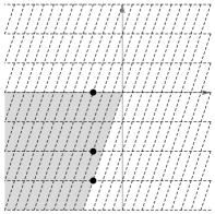
Figure 1. The polar lines (left) and resonant lines (right) when $A=$$\left[\begin{smallmatrix}1&1&1\\ 0&2&3\end{smallmatrix}\right]$. The opposites of the points of $A$ are highlighted. The shaded region is the domain of convergence of $M_{f}^{\Theta}(x,\beta)$.

Let $a_{i}$ denote the $i$th column of the matrix $A$, i.e., $a_{i}=\left[\begin{smallmatrix}1\\ k_{i}\end{smallmatrix}\right]$. The meromorphic extension of (2.1) is in this notation given by the extension formulas from [BFP12, (2.9)]:

$$M_{f}^{\Theta}(x,\beta)= \frac{-\beta_{2}}{\gamma_{0}\cdot\beta}\sum_{i=1}^{n}k_{i}\,x_{i}\,M_{f}^{\Theta}(x,\beta-a_{i})\quad\text{and}$$ (2.7)

$$M_{f}^{\Theta}(x,\beta)= \frac{-\beta_{2}}{\gamma_{k}\cdot\beta}\sum_{i=1}^{n}(k-k_{i})\,x_{i}\,M_{f}^{\Theta}(x,\beta-a_{i}).$$ (2.8)

The factor $k_{i}$ in (2.7) implies that the right hand side has a vanishing term for $i=1$, and similarly for $i=n$ in (2.8). This vanishing implies that (2.7) and (2.8) provide meromorphic extensions of $M_{f}^{\Theta}(x,\beta)$; the right hand side of (2.7) converges in the domain

$$\bigcap_{i=2}^{n}\left\{\beta\in{\mathbb{C}}^{2}\;\big{|}\;{\rm Re}(-\gamma_{0}\cdot(a_{i}+\beta))<0\,\text{ and }\,{\rm Re}(-\gamma_{k}\cdot(a_{i}+\beta))<0\right\},$$

which, since $k_{i}>0$ for $i>0$, is strictly greater than (2.2).

Applying the extension formula (2.7) a second time, the $i$th term of (2.7) is divided by the linear form

$$\gamma_{0}\cdot(\beta-a_{i})=(\gamma_{0}\cdot\beta)+\kappa,$$

where $\kappa=-\gamma_{0}\cdot a_{i}$ is a nonzero element of $G_{0}$. Repeated use of the extension formulas (2.7) and (2.8) yields an expression for the meromorphic extension of $M_{f}^{\Theta}(x,\beta)$ as a linear combination of shifted Euler–Mellin integrals, with coefficients that are products of reciprocals of distinct linear forms corresponding to resonant lines that belong to ${\rm Poles}(A)$.

Consequently, an expression for the extended Euler–Mellin integral $\Phi_{f}^{\Theta}(x,\beta)$ can, for each fixed $\beta$, be obtained from $M_{f}^{\Theta}(x,\beta)$ by iterations of the extension formulas (2.7) and (2.8). To do this, choices must be made as to the order in which the two types of extensions are performed. We focus on the two orderings given by either first extending over lines resonant with respect to the face $\{\left[\begin{smallmatrix}1\\ 0\end{smallmatrix}\right]\}$, and then extending over lines resonant with respect to the face $\{\left[\begin{smallmatrix}1\\ k\end{smallmatrix}\right]\}$, or vice versa.

If $\beta$ is contained in a polar line $L$ with defining equation $(\gamma_{j}\cdot\beta)-\kappa=0$, then restricting the entire function $\Psi_{f}^{\Theta}(x,\beta)$ in $\beta$ to $L$, the only terms in the iterated expansion of $M_{f}^{\Theta}(x,\beta)$ that do not vanish are those for which the linear form $(\gamma_{j}\cdot\beta)-\kappa$ appears in the denominators of their coefficients. Thus, in order to explain the behavior of $\Psi_{f}^{\Theta}$ at such resonant parameters, it is necessary to carefully track the combinatorics of the coefficients in the expansion process of $M_{f}^{\Theta}(x,\beta)$. This is of particular importance when the parameter $\beta$ is contained in the intersection of two polar lines.

We conclude this section by noting that when $A$ has the form (1.2) and $\beta$ is nonresonant (see Definition 1.1), then extended Euler–Mellin integrals form a basis of the solution space of $H_{A}(\beta)$ at any nonsingular $x\in{\mathbb{C}}^{n}$.

Theorem 2.3.

[BFP12, Proposition 5.1] The extended Euler–Mellin integrals $\{\Psi_{f}^{\Theta}(\beta,x)\}$ of Definition 2.2, where $\Theta$ ranges over a set of connected components of the complement of ${\mathscr{C}}(f)$, are linearly independent when $\beta\in{\mathbb{C}}^{2}\smallsetminus{\rm ResArr}(A)$ and

$$x\in V\mathrel{\vbox{\hbox{\scriptsize.}\hbox{\scriptsize.}}}=\{x\in{\mathbb{C}}^{n}\mid\max(|x_{2}|,\dots,|x_{n-1}|)\ll\min(|x_{1}|,|x_{n}|)\}\subseteq{\mathbb{C}}^{n}\smallsetminus\Sigma_{A}.$$

Hence, for any $\beta\in{\mathbb{C}}^{2}\smallsetminus{\rm ResArr}(A)$, such a collection of extended Euler–Mellin integrals can be analytically continued to form a basis of the solution space of the $A$-hypergeometric system $H_{A}(\beta)$ at any $x\in{\mathbb{C}}^{n}\smallsetminus\Sigma_{A}$.

Remark 2.4.

If $A$ is more general, so that it corresponds to a $(d-1)$-dimensional projective toric variety, where $d>2$, we are not aware of a proof that the set of integrals obtained from the components of the complement of the closure of ${\mathscr{C}}(f)$ are linearly independent. If this were the case, it still might happen that $A$ does not have ${\rm vol}(A)$-many associated extended Euler–Mellin integrals that could be used to form a basis of the solution space of some $H_{A}(\beta)$. Even if one works up to $\mathrm{GL}_{d}({\mathbb{Z}})$-equivalence, which induces an isomorphism on $A$-hypergeometric systems, this difficulty cannot always be overcome. For example, if $A$ is the matrix

$$A=\begin{bmatrix}1&1&1&1&1\\ 0&2&2&1&0\\ 0&0&2&3&3\end{bmatrix},$$ (2.9)

then the rank of ${\rm Sol}_{\bar{x}}(H(\beta))$ is $11$ for all parameters $\beta$. However, $10$ is the maximal number of connected components of the complement of the coamoeba of a polynomial

$$\hskip 113.81102ptf(z_{1},z_{2})=x_{1}+x_{2}z_{1}^{2}+x_{3}z_{1}^{2}z_{2}^{2}+x_{4}z_{1}z_{2}^{3}+x_{5}z_{2}^{3}.\hskip 113.81102pt\hexagon$$

3. Parametric derivatives and solution sheaves

In this section we discuss, in a general setting, the classical method of taking parametric derivatives to obtain solutions of differential equations at special values of the parameters. This technique gives a partial understanding of the parametric variation of solutions of $H_{A}(\beta)$, as shown in Corollary 3.6, which is a weaker version of Theorems 1.2.

Let $P_{1}(x,\partial),\dots,P_{m}(x,\partial)$ be linear partial differential operators in $D[\beta]$, the Weyl algebra on ${\mathbb{C}}^{n}$ with additional commuting variables $\beta=\beta_{1},\dots,\beta_{d}$. Let $\varphi_{1}(\beta),\dots,\varphi_{m}(\beta)$ be polynomial functions of $\beta\in{\mathbb{C}}^{d}$, viewed as elements of $D[\beta]$. Consider the system $H(\beta)$ of parametric linear partial differential equations given by

$$P_{i}(x,\partial)\bullet\Phi(x,\beta)=\varphi_{i}(\beta)\Phi(x,\beta),\qquad i=1,\dots,m.$$ (3.1)

We view $H(\beta)$ as a left ideal in $D[\beta]$ defined by the operators $P_{i}(x,\partial)-\varphi_{i}(\beta)$.

Assume further that $\Phi(x,\beta)$ is locally analytic for $x$ in an open set $V\subseteq{\mathbb{C}}^{n}$ and $\beta$ in a neighborhood $\mathcal{U}$ (in the analytic topology) of $\bar{\beta}\in{\mathbb{C}}^{d}$. For $\gamma\in{\mathbb{C}}^{d}$, denote by $\nabla_{\gamma}$ the differentiation operator with respect to $\beta$ in the direction of $\gamma$. Applying $\nabla_{\gamma}$ to both sides of (3.1) yields

$$P_{i}(x,\partial)\bullet\nabla_{\gamma}\Phi(x,\beta)=\nabla_{\gamma}\varphi_{i}(\beta)\cdot\Phi(x,\beta)+\varphi_{i}(\beta)\cdot\nabla_{\gamma}\Phi(x,\beta),\qquad i=1,\dots,m.$$

Thus, if $\bar{\beta}$ is such that $\Phi(x,\bar{\beta})\equiv 0$ for $x\in V$, then it follows that $\nabla_{\gamma}\Phi(x,\bar{\beta})$ solves (3.1) at $\beta=\bar{\beta}$. In this case, we say that $\nabla_{\gamma}\Phi(x,\bar{\beta})$ has been constructed from $\Phi(x,\bar{\beta})$ by taking parametric derivatives.

If the function $\nabla_{\gamma}\Phi(x,\beta)$ happens to vanish identically at $\beta=\bar{\beta}$, then the parametric derivative procedure can be iterated. We now state a sufficient condition for this algorithm to terminate after a finite number of steps. Note that the extended Euler–Mellin integrals provide a basis of solutions for $H_{A}(\beta)$ at nonsingular $x$ and nonresonant $\beta$ and thus satisfy the hypotheses of this result.

Proposition 3.1.

Let $\Phi(x,\beta)$ be a solution to (3.1), which is analytic in $x$ in an open subset $V\subseteq{\mathbb{C}}^{n}$, and locally analytic and not identically vanishing in a neighborhood ${\mathcal{U}}$ of $\bar{\beta}$. Assume further that $\Phi(x,\beta)$ is identically vanishing when $\beta$ is restricted to a hyperplane $L\subset{\mathbb{C}}^{d}$ containing $\bar{\beta}$. Then for each $\gamma\notin T_{L}(\bar{\beta})$, the tangent space of $L$ at $\bar{\beta}$, the above process terminates after a finite number of steps. That is, for each $\bar{\beta}$, there is an integer $q=q(\bar{\beta},\gamma)$ such that $\nabla_{\gamma}^{(q)}\Phi(x,\beta)\not\equiv 0$ for $\beta\in L\cap{\mathcal{U}}$. Furthermore, the number $q$ does not depend on $\gamma$, and thus it defines a function $\bar{\beta}\mapsto q(\bar{\beta})$, which in turn is upper semicontinuous in the analytic topology of ${\mathbb{C}}^{d}$.

Proof.

Let $v_{1},\dots,v_{d-1}\in T_{L}(\bar{\beta})$ extend by $\gamma$ to a basis of ${\mathbb{C}}^{d}$. Then

$$\nabla_{v_{i}}^{(q)}\Phi(x,\beta)\equiv 0\quad\text{for}\quad i\in\{1,\dots,d-1\},\quad q\geq 0,\quad\text{and}\quad\beta\in L\cap{\mathcal{U}}.$$

If in addition, $\nabla_{\gamma}^{(q)}\Phi(x,\beta)=0$ for all $q$ and $\beta\in L\cap{\mathcal{U}}$, then all mixed derivatives $\nabla_{v_{i}}^{(q_{i})}\nabla_{\gamma}^{(q)}\Phi(x,\beta)$ also vanish in $L\cap{\mathcal{U}}$; in particular, they vanish at $\bar{\beta}$. Hence Taylor’s formula implies that $\Phi(x,\beta)=0$ for all $\beta$ in a neighborhood of $\bar{\beta}$, a contradiction. That $q$ does not depend on $\gamma$ follows by a change of variables fixing $v_{1},\dots,v_{d-1}$. To see that the map $\bar{\beta}\mapsto q(\bar{\beta})$ is upper semicontinous, it is enough to note that $\nabla_{\gamma}^{(q)}\Phi(x,\beta)\not\equiv 0$ for $\beta\in L\cap{\mathcal{U}}$ implies that $\nabla_{\gamma}^{(q)}\Phi(x,\beta)\not\equiv 0$ for $\beta$ in some (analytic) open neighborhood of $\bar{\beta}$. ∎

Proposition 3.2.

With the hypotheses of Proposition 3.1, assume further that in a neighborhood ${\mathcal{V}}$ of $\bar{\beta}$, the function $\Phi(x,\beta)$ is not identically vanishing in $x$ for any fixed $\beta\in{\mathcal{V}}\smallsetminus L$. Then $\nabla_{\gamma}^{(q)}\Phi(x,\beta)$ is not identically vanishing in $x$ at $\bar{\beta}$.

Proof.

We can assume that $\gamma$ is the normal vector for the hyperplane $L$, so that $L$ is defined by a linear equation $\gamma\cdot\beta=\kappa$. By l’Hôpital’s rule, for $\beta\in{\mathcal{V}}\cap L$,

$$\nabla_{\gamma}^{(q)}\Phi(x,\beta)=\left.\Phi(x,\beta)((\gamma\cdot\beta)-\kappa)^{-q}\right.$$

Hence for $\beta\in{\mathcal{V}}\cap L$, the function $\nabla_{\gamma}^{(q)}\Phi(x,\beta)$ can be replaced by the analytic extension to $L$ of the ratio

$$\Phi(x,\beta)((\gamma\cdot\beta)-\kappa)^{-q},$$

which gives a solution of $H(\beta)$ that varies locally analytically in a neighborhood of $L$.

The vanishing locus of $\Phi(x,\beta)((\gamma\cdot\beta)-\kappa)^{-q}$ is an analytic subvariety of codimension at least $1$ in $L$. Thus, by assumption, this vanishing locus is of codimension at least $2$ in ${\mathbb{C}}^{d}$, which implies that it is empty. ∎

For any $\beta\in{\mathbb{C}}^{d}$, the characteristic variety of $H(\beta)$ is

$${\rm Char}(H(\beta))\mathrel{\vbox{\hbox{\scriptsize.}\hbox{\scriptsize.}}}={\rm Var}({\rm gr}^{F}(H(\beta)))\subseteq T^{*}{\mathbb{C}}^{n}\cong{\mathbb{C}}^{2n},$$ (3.2)

where $F$ is the order filtration on $D$, given by the order of differential operators. The singular locus of $H(\beta)$, denoted ${\rm Sing}(H(\beta))$, is the image under the projection $T^{*}{\mathbb{C}}^{n}\to{\mathbb{C}}^{n}$ given by $(x,\xi)\mapsto x$ of ${\rm Char}(H(\beta))\smallsetminus{\rm Var}(\xi_{1},\dots,\xi_{n})$. Given a generic nonsingular point $\bar{x}\in{\mathbb{C}}^{n}$ for $H(\beta)$, denote by $\mathcal{O}^{\rm an}_{{\mathbb{C}}^{n},\bar{x}}$ the space of multivalued germs of analytic functions at $\bar{x}$. The ${\mathbb{C}}$-vector space

$${\rm Sol}_{\bar{x}}(H(\beta))\mathrel{\vbox{\hbox{\scriptsize.}\hbox{\scriptsize.}}}=\{\Phi\in\mathcal{O}^{{\rm an}}_{{\mathbb{C}}^{n},\bar{x}}\mid Q\bullet\Phi=0\text{ for all }Q\in H(\beta)\}$$

is the solution space of $H(\beta)$ at $\bar{x}$.

We introduce one more notion before stating the main result of this section. Given a countable, locally finite union ${\mathscr{L}}$ of linear varieties in ${\mathbb{C}}^{d}$, let ${\mathcal{S}}({\mathscr{L}})$ denote the natural stratification of ${\mathbb{C}}^{d}$ induced by the flats of ${\mathscr{L}}$. In other words, the closure of a stratum of ${\mathcal{S}}({\mathscr{L}})$ is an intersection of irreducible components of ${\mathscr{L}}$, and ${\mathcal{S}}({\mathscr{L}})$ is the coarsest possible stratification of ${\mathbb{C}}^{d}$ with this property.

Theorem 3.3.

Consider a system $H(\beta)\subseteq D[\beta]$ of linear partial differential equations of the form (3.1). Suppose that there exists a countable, locally finite union ${\mathscr{L}}$ of linear varieties in ${\mathbb{C}}^{d}$ and an open set $V\subseteq{\mathbb{C}}^{n}$, disjoint from ${\rm Sing}(H(\beta))$ for all $\beta$, such that

$$\dim_{{\mathbb{C}}}({\rm Sol}_{\bar{x}}(H(\beta)))=r<\infty\text{ for all }\beta\notin{\mathscr{L}}\text{ and }x\in V.$$

Suppose further that there exists a set of functions that are locally analytic and form a basis of ${\rm Sol}_{x}(H(\beta))$ for $(x,\beta)\in V\times({\mathbb{C}}^{d}\smallsetminus{\mathscr{L}})$. Then along each stratum $S\in{\mathcal{S}}({\mathscr{L}})$, and for any $x\in V$, there is an $r$-dimensional subspace of ${\rm Sol}_{x}(H(\beta))$ which, when restricted to $S$, is locally analytic in $\beta$.

Proof.

Let $\Phi_{1}(x,\beta),\dots,\Phi_{r}(x,\beta)$ be a collection of solutions that are locally analytic and form a basis of ${\rm Sol}_{x}(H(\beta))$ for $(x,\beta)\in V\times({\mathbb{C}}^{d}\setminus{\mathscr{L}})$.

We first claim that it is enough to consider the case that ${\mathscr{L}}$ is a union of hyperplanes. To see this, let $K\subset{\mathscr{L}}$ be an irreducible component of ${\mathscr{L}}$ of codimension at least two, and let $K_{0}$ denote the unique maximal stratum of ${\mathcal{S}}({\mathscr{L}})$ that is contained in $K$. Since ${\mathscr{L}}$ is locally finite, $K_{0}$ is a nonempty Zariski open subset of $K$. Note that for any $\beta\in K_{0}$, there exists an analytic neighborhood $N$ of $\beta$ such that $N\cap K_{0}=N\cap K$ and furthermore, any linear combination of the functions $\Phi_{1},\dots,\Phi_{r}$ is analytic and nonvanishing for $\beta\in N\smallsetminus K$. Since $K$ is of codimension at least two, we conclude that any linear combination of $\Phi_{1},\dots,\Phi_{r}$ has a unique nonvanishing analytic continuation to $N$.

We may thus assume that ${\mathscr{L}}$ is a union of hyperplanes. To proceed with the proof, we use induction on $d$. The base case $d=0$ is trivial. Thus, assume now that the statement is proven for $d<k$, and consider the case $d=k$.

Proposition 3.1 can be applied to a collection of linearly independent solutions of the system $H(\beta)$ for all $\beta\in{\mathbb{C}}^{k}\smallsetminus{\mathscr{L}}$, as follows. If there is a linear combination

$$\Phi(x,\beta)=\sum_{i=1}^{r}c_{i}\Phi_{i}(x,\beta)$$

that encodes a linear dependence relation valid when $\beta\in L$, for some linear space $L\subseteq{\mathscr{L}}$, then Proposition 3.1 can be applied to the solution $\Phi(x,\beta)$. Further, if there are several linear dependencies that are valid along $L$, then Proposition 3.1 can be applied repeatedly.

Consider a hyperplane $L\subset{\mathscr{L}}$. Let ${{\mathscr{L}}}_{L}\subset L$ denote the set

$${\mathscr{L}}_{L}=\bigcup_{\begin{subarray}{c}S\in{\mathcal{S}}({\mathscr{L}})\\ \overline{S}\subsetneq L\end{subarray}}S.$$

Note that ${\mathscr{L}}_{L}$ is a countable, locally finite union of hyperplanes in $L\cong{\mathbb{C}}^{d-1}$. For a fixed $\bar{\beta}$ contained $L\smallsetminus{\mathscr{L}}_{L}$, Proposition 3.2 shows that the solutions obtained using Proposition 3.1 do not vanish identically in $x$ at $\bar{\beta}$. Thus, by Proposition 3.1, we obtain $r$ locally analytic functions which are nontrivial and linearly independent for $\beta\in L\smallsetminus{\mathscr{L}}_{L}$. Furthermore, the polynomial functions $\varphi_{i}(\beta)$, $i=1,\dots,m$, are still algebraic when restricted to the hyperplane $L$. In particular, by induction, for each stratum $S\in{\mathcal{S}}({\mathscr{L}}_{L})$, there is a set of $r$ linearly independent elements of ${\rm Sol}_{x}(H(\beta))$ for each $\beta\in S$, which are locally analytic.

Consider a stratum $S\in{\mathcal{S}}({\mathscr{L}})$ of codimension $c>1$. Such a stratum is the intersection of $L_{1},\dots,L_{c}$, which are hyperplanes in ${\mathscr{L}}$. By the previous paragraph, along each $L_{i}$, there is an $r$-dimensional solution space of $H(\beta)$ at $x\in V$ for all $\beta\in L_{i}$. In general, these solution spaces need not coincide along $S$; however, to complete this proof, it suffices to choose one of the available solution spaces for each such stratum $S$. ∎

Theorem 3.4.

Assume that the $A$-hypergeometric system $H_{A}(\beta)$ is such that the set of rank-jumping parameters ${\mathcal{E}}_{A}$ is at most zero-dimensional. Then there is a stratification of ${\mathbb{C}}^{d}$ such that for each stratum $S$, the solutions of $H_{A}(\beta)$ are locally analytic as functions of $x$ and $\beta$ in $({\mathbb{C}}^{n}\smallsetminus\Sigma_{A})\times S$.

Proof.

At nonresonant parameters $\beta$, there is a basis of the solution space of $H_{A}(\beta)$ given by Euler-type integrals over compact cycles [GKZ90, Theorem 2.10]. These compact cycles can be chosen uniformly for all parameters, so the corresponding integrals yield entire functions of the parameter $\beta$ (cf. Section 4). Applying Theorem 3.3 yields for each stratum $S\in{\mathcal{S}}({\rm ResArr}(A))$, a set of ${\rm vol}(A)$-many linearly independent solutions of $H_{A}(\beta)$ that are locally analytic for $(x,\beta)\in({\mathbb{C}}^{n}\smallsetminus\Sigma_{A})\times S$.

The proof is now complete if the set of rank-jumping parameters ${\mathcal{E}}_{A}$ is empty. If not, refine ${\mathcal{S}}({\rm ResArr}(A))$ by placing each rank-jumping parameter in its own stratum. Then at each $\beta\in{\mathcal{E}}_{A}$, complete a basis of elements of ${\rm Sol}_{x}(H_{A}(\beta))$ for $x\in{\mathbb{C}}^{n}\smallsetminus\Sigma_{A}$, as there is nothing to prove regarding analyticity in $\beta$ for such parameters because ${\mathcal{E}}_{A}$ is zero-dimensional. ∎

Corollary 3.5.

If ${\mathbb{C}}[\partial]/I_{A}$ is Cohen–Macaulay, then for any stratum $S\in{\mathcal{S}}({\rm ResArr}(A))$, the solutions of $H_{A}(\beta)$ are locally analytic as functions of $x$ and $\beta$ in $({\mathbb{C}}^{n}\smallsetminus\Sigma_{A})\times S$.

Proof.

When ${\mathbb{C}}[\partial]/I_{A}$ is Cohen–Macaulay, $H_{A}(\beta)$ has no rank jumping parameters [MMW05, Corollary 9.2]. Thus the result follows immediately from Theorem 3.4. ∎

Returning to the case of projective toric curves, the following is another consequence of Theorem 3.4.

Corollary 3.6.

Assume that $A$ has the form (1.2). Let $\mathcal{C}$ be the subset of ${\rm ResArr}(A)$ consisting of points lying on two resonant lines, and form a decomposition ${\mathbb{C}}^{2}=({\mathbb{C}}^{2}\smallsetminus{\rm ResArr}(A))\cup({\rm ResArr}(A)\smallsetminus\mathcal{C})\cup\mathcal{C}$. Then the solutions of $H_{A}(\beta)$ are locally analytic as functions of $x$ and $\beta$ on $({\mathbb{C}}^{n}\smallsetminus\Sigma_{A})\times({\mathbb{C}}^{2}\smallsetminus{\rm ResArr}(A))$ and also on $({\mathbb{C}}^{n}\smallsetminus\Sigma_{A})\times({\rm ResArr}(A)\smallsetminus\mathcal{C})$.

In Corollary 3.6, note that it might be possible to take a strictly smaller union of lines, as we show in Theorem 1.3.

Remark 3.7.

If ${\mathcal{E}}_{A}$ is not zero-dimensional, then Theorem 3.3 cannot be used to explain how to create (and control with respect to $\beta$) additional linearly independent solutions along higher-dimensional components of ${\mathcal{E}}_{A}$. Further tools are being developed to address this issue. $\hexagon$

Although Corollary 3.6 provides information on the parametric behavior of the solutions of a hypergeometric system associated to a projective toric curve, this information is not very explicit, and in particular, does not involve the formation of rank jumps. In the upcoming sections, we work towards the significantly stronger Theorems 1.2 and 1.3.

4. Resonant parameters and Euler–Mellin integrals

In this section, we study the behavior of extended Euler–Mellin integrals at parameters that are resonant with respect to precisely one facet of $A$, see Definition 1.1. We obtain an explicit understanding of how these solutions behave along a line in ${\rm Poles}(A)$, while the behavior along nonpolar lines seems to be fundamentally different.

We first consider the case that $\beta$ is polar, where the behavior is illustrated by the following example. A series solution $\sum_{v\in{\mathbb{C}}^{n}}c_{v}x^{v}$ of $H_{A}(\beta)$ is said to have finite support if the set $\{v\in{\mathbb{C}}^{n}\mid c_{v}\neq 0\}$ is finite.

Example 4.1.

For any $A$ as in (1.2), consider the supporting line of the cone (2.2) given by $\beta_{2}=0$, which is contained in ${\rm Poles}(A)$. In order to evaluate $\Psi_{f}^{\Theta}$, we must expand $M_{f}^{\Theta}(x,\beta)$ once in the direction of $\mu_{0}$, which yields

$$M_{f}^{\Theta}(x,\beta)=\frac{\beta_{1}}{\beta_{2}}\int_{\operatorname{Arg}^{-1}(\theta)}z^{-\beta_{2}+1}\frac{f^{\prime}(z)}{f(z)^{-\beta_{1}+1}}\,\frac{dz}{z},$$

for $\theta\in\Theta$. Hence, along the line $\beta_{2}=0$, the Euler–Mellin integral for $\Theta$ evaluates, after applying an extension formula once, as follows:

$$\left.\frac{M_{f}^{\Theta}(x,\beta)}{\Gamma(\beta_{2})}\right|_{\beta_{2}=0}=\beta_{1}\int_{\operatorname{Arg}^{-1}(\theta)}\frac{f^{\prime}(z)}{f(z)^{-\beta_{1}+1}}\,dz=\beta_{1}f(0)^{\beta_{1}}=\beta_{1}x_{1}^{\beta_{1}}.$$

Most notably, $\Psi_{f}^{\Theta}(\beta_{1},0)$ is independent of $\Theta$ and equal to a series solution of $H_{A}(\beta)$ with finite support. $\hexagon$

Theorem 4.2.

If $L$ is a line contained in ${\rm Poles}(A)$, then for all $\beta\in L$, all extended Euler–Mellin integrals $\Psi_{f}^{\Theta}(x,\beta)$ coincide and evaluate to a finitely supported series solution of $H_{A}(\beta)$. After possibly removing a factor which is constant with respect to $x$, this series is nonvanishing in $x$ for each $\beta$ and varies locally analytically on $({\mathbb{C}}^{n}\smallsetminus{\rm Var}(x_{1}x_{n}))\times L$.

Proof.

It is enough to consider $x\in V$ as in Theorem 2.3. We first consider the case $\beta_{2}=N$, for some integer $N$, so that $L=L_{0}(N)$ is an integer translate of the span of the face $\left\{\left[\begin{smallmatrix}1\\ 0\end{smallmatrix}\right]\right\}$. From (2.5), since $L\subseteq{\rm Poles}(A)$, there exists a partition of $N$ using only $k_{2},\dots,k_{n}$. Let $P(A,N)$ denote the set of all ordered partitions $p$ of $N$ with parts $k_{2},\dots,k_{n}$. Let $m_{i}(p)$ denote the number of times $k_{i}$ appears in $p$, and set $m(p)\mathrel{\vbox{\hbox{\scriptsize.}\hbox{\scriptsize.}}}=(m_{1}(p),\dots,m_{n}(p))$, so that $|m(p)|$ is the length of $p$. Furthermore, for each $i\in\{1,\dots,|m(p)|\}$, let $s_{i}\mathrel{\vbox{\hbox{\scriptsize.}\hbox{\scriptsize.}}}=s_{i}(p)$ denote the $i$th partial sum of $p$. Now parameterize the line $L_{0}(N)=\{\beta\in{\mathbb{C}}^{2}\mid\beta_{2}=N\}$ by

$$\lambda\mapsto(\lambda,N)\quad\text{for}\quad\lambda\in{\mathbb{C}}.$$

We claim that, for each connected component $\Theta$ of the complement of ${\mathscr{C}}(f)$, the Euler–Mellin integral for $\Theta$ evaluates, after applying the extension formulas, to

$$\left.\frac{M_{f}^{\Theta}(x,\beta)}{\Gamma(\beta_{2})}\right|_{L_{0}(N)}=x_{1}^{\lambda}\sum_{p\in P(A,N)}\left(\prod_{i=1}^{|m(p)|-1}\frac{\lambda-i}{N-s_{i}(p)}\right)\left(\prod_{i=2}^{n}k_{i}^{m_{i}(p)}\left(\frac{x_{i}}{x_{1}}\right)^{m_{i}(p)}\right).$$ (4.1)

Indeed, the factor $\Gamma(\beta_{2})$ in (2.5) implies that the only terms in the expansion of $M_{f}^{\Theta}(x,\beta)$ that are relevant at $\beta_{2}=N$ are those containing the factor $\beta_{2}-N$ in the denominators of their coefficients. This is the case only for terms corresponding to ordered partitions of $N$, and the term corresponding to $p\in P(A,N)$, when restricted to $L_{0}(N)$, is the one given in (4.1), including the monomial $x^{m(p)}$. The integral of this term evaluates, in the manner of Example 4.1, to $x_{1}^{\beta_{1}-|m(p)|}$.

By symmetry, a similar formula can be given when $k\beta_{1}-\beta_{2}=N$, so that $L=L_{k}(N)$ is a translate of the span of the face $\left\{\left[\begin{smallmatrix}1\\ k\end{smallmatrix}\right]\right\}$. In this case, consider the parameterization of $L_{k}(N)$ given by

$$\lambda\mapsto(\lambda,k\lambda+N)\quad\text{for}\quad\lambda\in{\mathbb{C}}.$$

The analog of (4.1) for this line is

$$\left.\frac{M_{f}^{\Theta}(x,\beta)}{\Gamma(k\beta_{1}-\beta_{2})}\right|_{L_{k}(N)}=x_{n}^{\lambda}\sum_{p\in P(\bar{A},N)}\left(\prod_{i=1}^{|m(p)|-1}\frac{\lambda-i}{N-s_{i}(p)}\right)\,\left(\prod_{i=1}^{n-1}(k-k_{i})^{m_{i}(p)}\left(\frac{x_{i}}{x_{n}}\right)^{m_{i}(p)}\right).$$ (4.2)

Now the coefficient of a monomial $x_{1}^{\lambda-|m_{p}|}\prod_{i=2}^{n}x_{i}^{m_{i}(p)}$ in (4.1) or $x_{n}^{\lambda-|m_{p}|}\prod_{i=2}^{n-1}x_{i}^{m_{i}(p)}$ in (4.2) is a sum of positive multiples of the product

$$\prod_{i=1}^{|m(p)|-1}(\lambda-i),$$ (4.3)

and hence it is a positive multiple of (4.3); in particular, the coefficient of a monomial vanishes only if the product (4.3) vanishes. Thus a function of the form (4.1) or (4.2) is nontrivial unless $\lambda$ is such that all the coefficients vanish, which is equivalent to $\lambda$ being a positive integer such that every $p\in P(A,N)$ has more than $\lambda$ terms. However, this vanishing can be removed, as it is caused by a factor $(\lambda-i)$ appearing in all coefficients of (4.1) or (4.2). Removing such factors, (4.1) and (4.2) provide everywhere nontrivial solutions that vary locally analytically in $\lambda$ along $L_{0}(N)$ or $L_{k}(N)$, respectively. Local analyticity on ${\mathbb{C}}^{n}\smallsetminus{\rm Var}(x_{1}x_{n})$ is clear from the denominators of (4.1) and (4.2). ∎

The behavior of extended Euler–Mellin integrals along nonpolar resonant lines is more difficult to track. To illustrate the difference, we turn to a discussion of the behavior of residue integrals.

Still using $f(z)=\sum_{i=1}^{n}x_{i}z^{k_{i}}$, consider an integral of the form

$$\int_{C}{f(z)^{\beta_{1}}}{z^{-\beta_{2}}}\,\,\frac{dz}{z},$$ (4.4)

where $C$ is some cycle in ${\mathbb{C}}\smallsetminus{\rm Var}(f)$. It is shown in [GKZ90, Theorem 2.7] that (4.4) is $A$-hypergeometric as a germ in $x$, provided that it has sufficiently nice convergence properties. This is the case when $C$ is compact. The integrand in (4.4) has, for very general $\beta$ (including all nonresonant parameters), singularities at $0$, $\infty$, and at each $\rho\in{\rm Var}(f)$. This yields ${\rm vol}(A)+2$ residue integrals

$${\rm Res}_{\rho}(x,\beta)\mathrel{\vbox{\hbox{\scriptsize.}\hbox{\scriptsize.}}}=\int_{C(\rho)}{f(z)^{\beta_{1}}}{z^{-\beta_{2}}}\,\,\frac{dz}{z},$$

where $C(\rho)$ is a small counterclockwise loop around $\rho$ if $\rho\in{\mathbb{C}}$ equals zero or a root of $f$, or it is a large clockwise oriented loop if $\rho=\infty$. The integral (4.4) is multivalued in two senses. It is multivalued in $x$, as an analytic continuation along a loop in $({\mathbb{C}}^{*})^{n}$ need not preserve the cycle $C$; also, it depends on the choices of branches of the exponential functions $f(z)^{\beta_{1}}$ and $z^{-\beta_{2}}$. Note that the values of (4.4) for different branches of these exponential functions differ only by multiplication times an exponential function in the parameters. In particular, for a fixed cycle $C$, the ${\mathbb{C}}$-vector space spanned by the integral in question is uniquely determined. In the case when its cycle of integration $C$ is compact, (4.4) is entire in $\beta$, as its integrand shares this property.

Convention 4.3.

Let $\rho_{1},\dots,\rho_{k}$ denote the zeros of $f$, with indices considered modulo $k={\rm vol}(A)$, ordered by their arguments. Similarly, label the components of the complement of ${\mathscr{C}}(f)$ by $\Theta_{i}$, where the indexing is chosen so that the sector $\operatorname{Arg}^{-1}(\Theta_{i})$ contains $\rho_{i-1}$ and $\rho_{i}$ in its boundary.

Because of the multivaluedness of (4.4), at generic $\beta$, the vanishing theorem of residues does not apply. However, for parameters $\beta$ contained in (2.2), it follows from the estimates in the proof of [BFP12, Theorem 2.3] that for each $\rho_{i}\in{\rm Var}(f)$,

$${\rm Res}_{\rho_{i}}(x,\beta)=M_{f}^{\Theta_{i}}(x,\beta)-M_{f}^{\Theta_{i+1}}(x,\beta),$$ (4.5)

provided that the branches of (the integrands of) the Euler–Mellin integrals in the right hand side are chosen consistently. Note that by the uniqueness of meromorphic extension, this equality holds for all nonresonant $\beta$, when on the right hand side, each $M_{f}^{\Theta_{j}}(x,\beta)$ is replaced by $\Psi_{f}^{\Theta_{j}}(x,\beta)$.

It is natural to decompose the set of residue integrals into two types, where the first is given by the residues at the roots $\rho\in{\rm Var}(f)$ and the second is given by the residues at $0$ and $\infty$. As we now show, along polar lines, the first type of residue integrals vanish; however, along nonpolar resonant lines, it is instead the residue integrals of the second type that vanish.

Proposition 4.4.

1. If $\beta\in{\rm Poles}(A)$, then ${\rm Res}_{\rho}(x,\beta)=0$ for each $\rho\in{\rm Var}(f)$.

2. If $\beta\in{\rm ResArr}(A)\smallsetminus{\rm Poles}(A)$, then at least one of ${\rm Res}_{0}(x,\beta)$ and ${\rm Res}_{\infty}(x,\beta)$ vanishes identically in $x$.

Proof.

Note that (1) follows from (4.5) and Theorem 4.2.

For (2), it is enough to consider the case $\beta_{2}=N$ for some $N\in{\mathbb{Z}}$, so that $\beta$ is resonant with respect to the face $\left\{\left[\begin{smallmatrix}1\\ 0\end{smallmatrix}\right]\right\}$. (If $\beta$ is instead resonant with respect to the face $\left\{\left[\begin{smallmatrix}1\\ k\end{smallmatrix}\right]\right\}$, then apply the change of variables given by $z\mapsto 1/z$ to return to this case.)

We claim that ${\rm Res}_{0}(x,\beta)$ vanishes identically in $x$. If $N$ is a nonpositive integer, then the integrand of (2.1) is analytic in a neighborhood of $z=0$. Thus, the only case to consider is when $N$ is positive, which corresponds to a gap in the set ${\rm Poles}(A)$ of polar lines.

Since residue integrals involve compact cycles, they converge for every $\beta$. However, by uniqueness of meromorphic extension, the identities (2.7) and (2.8) hold. Hence

$${\rm Res}_{0}(x,\beta)=\frac{\beta_{1}}{\beta_{2}}\int_{C(0)}z^{-\beta_{2}+1}f^{\prime}(z)f(z)^{\beta_{1}-1}\,\frac{dz}{z},$$

where $f^{\prime}(z)$ denotes the derivative of $f(z)$ with respect to $z$. By applying this formula repeatedly, we conclude that it is enough to show that each term of $f^{\prime}(z)$ which corresponds to $k_{i}>\beta_{1}$ vanishes. Indeed, this term equals

$$\frac{\beta_{1}}{\beta_{2}}\int_{C(0)}z^{-\beta_{2}+1}k_{i}z_{i}^{k_{i}-1}f(z)^{\beta_{1}-1}\,\frac{dz}{z},$$

whose integrand has a zero at the origin of order $k_{i}-\beta_{1}-1\geq 0$. ∎

Remark 4.5.

It is not clear if any further dependencies of the residue integrals exist at nonpolar resonant parameters. Thus, the implications of Proposition 4.4.(2) for extended Euler–Mellin integrals also remain unclear. Computational evidence suggests that at nonpolar resonant parameters, the analytic continuations of the extended Euler–Mellin integrals remain linearly independent. If this statement were proven, then the decomposition of ${\mathbb{C}}^{2}$ in Theorem 1.2 could instead be given as $({\mathbb{C}}^{2}\smallsetminus{\rm Poles}(A))\cup{\rm Poles}(A)$. On the other hand, all the lines in the arrangement ${\mathscr{L}}$ from Theorem 1.3 are polar, a fact that is proved using hypergeometric series. $\hexagon$

5. Intersections of polar lines and Euler–Mellin integrals

In this section, we explain the behavior of extended Euler–Mellin integrals at parameters $\beta$ that lie at the intersection of two resonant lines, so that $\beta$ is resonant with respect to both faces of $A$, see Definition 1.1. The partition of the resonant arrangement into polar and nonpolar lines gives a natural partition of these parameters into three distinct cases.

At intersections of two nonpolar lines, and also at intersections of one polar and one nonpolar line, the rank of $H_{A}(\beta)$ is ${\rm vol}(A)=k$. As discussed in Remark 4.5, it not clear how (or if) the extended Euler–Mellin integrals form linear dependencies at such parameters. We resolve this issue later through the use of series solutions of $H_{A}(\beta)$ in Theorem 6.2.

Thus for now, we consider only the third case, when a parameter $\beta$ is contained in the intersection of two polar lines, which, in particular, includes all rank-jumping parameters. Associated to these two lines, respectively, are the two finitely supported series as described in Theorem 4.2. Before we (possibly) remove unnecessary (vanishing) coefficients at the end of the proof of Theorem 4.2, these two series are evaluations of the same integral and therefore coincide. However, after such coefficients are removed, the resulting two series may or may not coincide. For $\beta\in{\mathbb{Z}}^{2}$, this is decided by whether or not $\beta$ is rank-jumping.

Recall that ${\mathcal{E}}_{A}\mathrel{\vbox{\hbox{\scriptsize.}\hbox{\scriptsize.}}}=\{\beta\in{\mathbb{C}}^{2}\mid{\rm rank}\,H_{A}(\beta)>{\rm vol}(A)\}$ denotes the set of rank-jumping parameters.

Theorem 5.1.

Suppose that $\beta$ is at the intersection of two resonant lines, both of which are contained in ${\rm Poles}(A)$.

1. If $\beta\notin{\mathbb{Z}}^{2}$ or $\beta\in{\mathcal{E}}_{A}$, then the two solutions obtained in Theorem 4.2 at $\beta$ are finitely supported and linearly independent.

2. If $\beta\in{\mathbb{Z}}^{2}\smallsetminus{\mathcal{E}}_{A}$, then for $x\in({\mathbb{C}}^{n}\smallsetminus\Sigma_{A})$, then the two solutions obtained in Theorem 4.2 at $\beta$ coincide and equal a single finitely supported series.

If $\beta\in{\mathbb{N}}A$, [SST00, Lemma 3.4.10] (or [CDD99, Proposition 1.1]) show that $H_{A}(\beta)$ has a unique (up to multiplication by a constant) polynomial solution. By Theorem 5.1, this solution is given by an extended Euler–Mellin integral.

Example 5.2.

We compute the finitely supported solutions provided by Theorem 4.2 when $A=\left[\begin{smallmatrix}1&1&1&1\\ 0&1&3&4\end{smallmatrix}\right]$. At $\beta=\left[\begin{smallmatrix}1\\ 1\end{smallmatrix}\right]\in{\mathbb{N}}A$, (4.1) and (4.2) both produce $x_{1}$. Next, at $\beta=\left[\begin{smallmatrix}1/2\\ 1\end{smallmatrix}\right]$, they yield the two finitely supported Puiseux series $x_{1}^{-\frac{1}{2}}x_{2}$ and $x_{3}x_{4}^{-\frac{1}{2}}$. Finally, at the unique rank-jumping parameter for this $A$, $\beta=\left[\begin{smallmatrix}1\\ 2\end{smallmatrix}\right]$, they provide the two Laurent monomials $x_{1}^{-1}x_{2}^{2}$ and $x_{3}^{2}x_{4}^{-1}$. $\hexagon$

The support of a series solution $\sum_{v\in{\mathbb{C}}^{n}}c_{v}x^{v}$ of $H_{A}(\beta)$ is the set $\{v\in{\mathbb{C}}^{n}\mid c_{v}\neq 0\}$, and the negative support of a monomial $c_{v}x^{v}$ is the set $\{i\mid v_{i}\in{\mathbb{Z}}_{<0}\}$.

Proof of Theorem 5.1.

If $\beta\notin{\mathbb{Z}}^{2}$, then the series solutions (4.1) and (4.2) of $H_{A}(\beta)$ have disjoint supports. In particular, they are linearly independent, and the only function which is simultaneously a constant multiple of both is the trivial (identically zero) function.

To handle the case $\beta\in{\mathbb{Z}}^{2}$, consider the matrix $\Delta\mathrel{\vbox{\hbox{\scriptsize.}\hbox{\scriptsize.}}}=CA$, where $C=\left[\begin{smallmatrix}k&-1\\ 0&\phantom{-}1\end{smallmatrix}\right]$. Since $C\in\mathrm{GL}_{2}({\mathbb{Q}})$, it induces an isomorphism of $A$-hypergeometric systems for any $\beta\in{\mathbb{C}}^{2}$:

$$H_{A}(\beta)\cong H_{\Delta}(\gamma)\quad\text{where $\gamma\mathrel{\vbox{\hbox{\scriptsize.}\hbox{\scriptsize.}}}=C\beta$}.$$

Figure 2 illustrates the change of coordinates induced by $C$ on the parameter space. Let ${\mathbb{N}}\Delta$ denote the monoid spanned by the columns of $\Delta$.

   

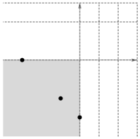
Figure 2. The left diagram shows ${\rm Poles}(A)$, while the right shows ${\rm Poles}(\Delta)$, mimicking Figure 1.

With this notation, when $\beta\in{\mathbb{Z}}^{2}$ is contained in two lines of ${\rm Poles}(A)$, consider all sets (if any) of the form $\{\delta^{i,j}\in{\mathbb{N}}\Delta\mid 1\leq i,j\leq 2\}$ such that, with $\gamma=C\beta$, all of the following hold:

$$\delta^{1,1}_{1}=\gamma_{1},\quad\delta^{1,1}_{2}+\delta^{1,2}_{2}=\gamma_{2},\quad\delta^{1,2}\neq\left[\begin{smallmatrix}0\\ 0\end{smallmatrix}\right],$$ (5.1)

$$\delta^{2,1}_{2}=\gamma_{2},\quad\delta^{2,1}_{1}+\delta^{2,2}_{1}=\gamma_{1},\quad\delta^{2,2}\neq\left[\begin{smallmatrix}0\\ 0\end{smallmatrix}\right].$$ (5.2)

The conditions (5.1) and (5.2) are necessary for the equations of the polar lines containing $\beta$ to appear in the coefficient of some term after the Euler–Mellin integrals have been expanded either first over the face $\{\left[\begin{smallmatrix}1\\ 0\end{smallmatrix}\right]\}$, or first over the face $\{\left[\begin{smallmatrix}1\\ k\end{smallmatrix}\right]\}$ respectively. From this, we immediately conclude that if there is no set of the form $\{\delta^{i,j}\in{\mathbb{N}}\Delta\mid 1\leq i,j\leq 2\}$ such that (5.1) and (5.2) hold, then all extended Euler–Mellin integrals vanish.

Let us now show that when $\beta\in{\mathbb{Z}}^{2}$, all extended Euler–Mellin integrals vanish at $\beta$ if and only if $\beta$ is rank-jumping for $A$. We first claim that, as $\beta\in{\mathbb{Z}}^{2}$ is contained in the intersection of two lines in ${\rm Poles}(A)$, there exists a pair $(\delta^{1,1},\delta^{1,2})$ such that (5.1) holds if and only if there exists a pair $(\delta^{2,1},\delta^{2,2})$ such that (5.2) holds. To see this, recall that $\Delta=CA$ and $\gamma=C\beta$, for $C$ as above, so $\beta\in{\mathbb{N}}A$ if and only if $\gamma\in{\mathbb{N}}\Delta$. Further, by symmetry, it is enough to show that (5.1) is equivalent to $\gamma\in{\mathbb{N}}\Delta$. Notice that each $\delta\in{\mathbb{N}}\Delta$ fulfills that $\delta_{1}+\delta_{2}=kl$, for some $l\in{\mathbb{N}}$. This implies that if $\delta$ and $\tilde{\delta}$ are such that $\delta_{1}=\tilde{\delta}_{1}$, then $\delta=\tilde{\delta}+h\left[\begin{smallmatrix}0\\ k\end{smallmatrix}\right]$ for some $h\in{\mathbb{Z}}$. If $(\delta^{1,1},\delta^{1,2})$ satisfies (5.1), then $\delta_{1}^{1,1}=\gamma_{1}$ and $\delta_{2}^{1,1}\leq\gamma_{2}$. Hence, $\gamma=\delta_{1}+h\left[\begin{smallmatrix}0\\ k\end{smallmatrix}\right]$ for some $h\geq 0$. Since $\left[\begin{smallmatrix}0\\ k\end{smallmatrix}\right]\in\Delta$, $\gamma\in{\mathbb{N}}\Delta$. Conversely, if $\gamma\in{\mathbb{N}}\Delta$, then because $\left[\begin{smallmatrix}k\\ 0\end{smallmatrix}\right]\in\Delta$, $\delta^{1,1}=\gamma$ and $\delta^{1,2}=\left[\begin{smallmatrix}k\\ 0\end{smallmatrix}\right]$ satisfies (5.1). This establishes the proof of the claim.

From the above calculation, we see that the failure of (5.1) is equivalent to $\beta\in\left({\mathbb{Z}}\left[\begin{smallmatrix}1\\ 0\end{smallmatrix}\right]+{\mathbb{N}}A\right)\smallsetminus{\mathbb{N}}A$. Similarly, the failure of (5.2) is equivalent to $\beta\in\left({\mathbb{Z}}\left[\begin{smallmatrix}1\\ k\end{smallmatrix}\right]+{\mathbb{N}}A\right)\smallsetminus{\mathbb{N}}A$. Thus the desired conclusion for $\beta\in{\mathbb{Z}}^{2}\smallsetminus{\mathcal{E}}_{A}$ follows from (1.4).

Finally, if $\beta\in{\mathcal{E}}_{A}$, we must show that the two finitely supported solutions recovered from (4.1) and (4.2) are linearly independent. Expressions for the two Laurent polynomial solutions at rank-jumping parameters are known from [CDD99], and they are identified by the negative supports of their monomials. One solution, which by necessity is obtained from (4.1), contains negative powers only of $x_{1}$. The other, by necessity is obtained from (4.2), contains negative powers only of $x_{n}$, establishing the result. ∎

6. Series solutions of hypergeometric systems on projective toric curves

The results of Sections 4 and 5 show that, when beginning with analytic continuations of extended Euler–Mellin integrals, it is necessary to take parametric derivatives as in Section 3 to complete a basis of the solution space of $H_{A}(\beta)$ at resonant parameters $\beta$. However, this technique is not sufficient to provide the statements of Theorems 1.2 and 1.3, since it could be the case that along a resonant line, some solution in a basis obtained via parametric derivatives vanished at a point resonant with respect to both facets of $A$. To circumvent this issue, in this section we make use of series solutions of $H_{A}(\beta)$, with the goal of proving the following two results.

Theorem 6.1.

If $L$ is a line contained in ${\rm ResArr}(A)$, then there exist ${\rm vol}(A)=k$ functions that are linearly independent solutions of $H_{A}(\beta)$ for all $\beta\in L$ and are locally analytic on $({\mathbb{C}}^{n}\smallsetminus\Sigma_{A})\times L$.

Theorem 6.2.

If $\bar{\beta}\in{\mathbb{Z}}^{2}$, there exists a neighborhood ${\mathcal{W}}$ of $\bar{\beta}$ in ${\mathbb{C}}^{2}$ and ${\rm vol}(A)-1$ functions satisfying the following:

1. they are solutions of $H_{A}(\beta)$ for all $\beta\in{\mathcal{W}}$,

2. they are locally analytic for $(x,\beta)\in({\mathbb{C}}^{n}\smallsetminus\Sigma_{A})\times{\mathcal{W}}$,

3. they are linearly independent, and

4. for any fixed $\beta\in{\mathcal{W}}$, the span of the specializations at $\beta$ of these functions does not contain any solution of $H_{A}(\beta)$ for which there exists an expression as a finitely supported series.

To obtain these results, we draw heavily on techniques developed in the influential book [SST00] by Saito, Sturmfels, and Takayama, especially Sections 2.5, 3.2, 3.4, and 4.2 of that text.

A weight vector $w\in{\mathbb{R}}_{\geq 0}^{n}$ induces a partial ordering $\preceq_{w}$ of the monomials in ${\mathbb{C}}[\partial]\mathrel{\vbox{\hbox{\scriptsize.}\hbox{\scriptsize.}}}={\mathbb{C}}[\partial_{1},\dots,\partial_{n}]$ via $\partial^{\nu}\preceq_{w}\partial^{\nu^{\prime}}$ if $w\cdot\nu\leq w\cdot\nu^{\prime}$. If $w$ is generic, then the ideal ${\rm in}_{w}(I_{A})$ generated by the leading terms of the elements of $I_{A}$ with respect to $w$ is a monomial ideal. Moreover, given any monomial order $\prec$ in ${\mathbb{C}}[\partial]$, then there exists $w\in{\mathbb{R}}_{\geq 0}^{n}$ such that ${\rm in}_{\prec}(I_{A})={\rm in}_{w}(I_{A})$.

Let $w\in{\mathbb{R}}_{\geq 0}^{n}$ be a generic weight vector. The ideal

$${\rm fin}_{w}(H_{A}(\beta))\mathrel{\vbox{\hbox{\scriptsize.}\hbox{\scriptsize.}}}={\rm in}_{w}(I_{A})+\langle E-\beta\rangle\subseteq D$$

is called the fake initial ideal of $H_{A}(\beta)$ with respect to $w$. If a monomial function $x^{v}$, with $v\in{\mathbb{C}}^{n}$ is a solution of ${\rm fin}_{w}(H_{A}(\beta))$, then $v$ is a fake exponent of $H_{A}(\beta)$ with respect to $w$.

If $w$ is a generic weight vector, $\preceq_{w}$ can be extended to $D$ via $x^{u}\partial^{\nu}\preceq_{w}x^{u^{\prime}}\partial^{\nu^{\prime}}$ whenever $-w\cdot u+w\cdot\nu\leq-w\cdot u^{\prime}+w\cdot\nu^{\prime}$. The initial ideal of $H_{A}(\beta)$ with respect to $w$, denoted ${\rm in}_{(-w,w)}H_{A}(\beta)$, is defined using this ordering, and it clearly contains ${\rm fin}_{w}(H_{A}(\beta))$. The exponents of $H_{A}(\beta)$ arise from the monomial solutions of ${\rm in}_{(-w,w)}H_{A}(\beta)$, and therefore all exponents of $H_{A}(\beta)$ are fake exponents.

Let $I\subseteq{\mathbb{C}}[\partial]$ be a monomial ideal. Then $\partial^{r}$ is a standard monomial of $I$ if $\partial^{r}\notin I$. A pair $(r,\sigma)$, where $r\in{\mathbb{N}}^{n}$ and $\sigma\subseteq\{1,\dots,n\}$, is a standard pair of $I$ if

1. $r_{j}=0$ for $j\in\sigma$,

2. for each $u\in{\mathbb{N}}^{n}$ with $u_{j}=0$ for $j\notin\sigma$, the monomial $\partial^{r}\partial^{u}$ is a standard monomial of $I$,

3. for each $\ell\notin\sigma$, there exists $u\in{\mathbb{N}}^{n}$ with $u_{j}=0$ for $j\notin\sigma\cup\{\ell\}$ such that $\partial^{r}\partial^{u}\in I$.

By [SST00, Lemma 4.1.3], fake exponents can be easily computed from standard pairs. More explicitly, for each standard pair $(r,\sigma)$ of ${\rm in}_{w}(I_{A})$, if there exists $v\in{\mathbb{C}}^{n}$ such that $Av=\beta$ and $v_{i}=r_{i}$ for $i\notin\sigma$ (such a $v$ is unique if it exists), then $v$ is a fake exponent of $H_{A}(\beta)$ with respect to $w$, and all such fake exponents arise this way.

Now fix $w$ representing the reverse lexicographic ordering $\partial_{1}\prec\partial_{n}\prec\partial_{n-1}\prec\cdots\prec\partial_{3}\prec\partial_{2}$ for $I_{A}$. Then the standard pairs of ${\rm in}_{w}(I_{A})$ in this case are of the form $(r,\{1,n\})$ (there are ${\rm vol}(A)=k$ of these top-dimensional standard pairs) and $(r,\{1\})$. See [SST00, Section 4.2] for more details.

Lemma 6.3.

Let $\beta\in{\mathbb{C}}^{2}$ and let $r,r^{\prime}\in{\mathbb{N}}^{n}$ be such that $(r,\{1,n\})$ and $(r^{\prime},\{1,n\})$ are top-dimensional standard pairs of ${\rm in}_{w}(I_{A})$. Denote by $v(\beta)$ and $v^{\prime}(\beta)$ the fake exponents of $H_{A}(\beta)$ associated to $(r,\{1,n\})$ and $(r^{\prime},\{1,n\})$, respectively. Then $v^{\prime}(\beta)-v(\beta)\notin{\mathbb{Z}}^{n}$.

Proof.

By contradiction, assume that $v^{\prime}(\beta)-v(\beta)=u\in{\mathbb{Z}}^{n}$. In particular, $Au=0$, and therefore $\partial^{u_{+}}-\partial^{u_{-}}\in I_{A}$. The initial form ${\rm in}_{w}(\partial^{u_{+}}-\partial^{u_{-}})$ belongs to the monomial ideal ${\rm in}_{w}(I_{A})$, so we may assume that $\partial^{u_{+}}\in{\rm in}_{w}(I_{A})$. (If $\partial^{u_{-}}$ is the lead term, then interchange the roles of $v^{\prime}(\beta)$ and $v(\beta)$; if $w\cdot u=0$, then both monomials must belong to the initial ideal.)

Note that $v^{\prime}(\beta)+u_{+}=v(\beta)+u_{-}$. Since the supports of $u_{+}$ and $u_{-}$ are disjoint, $\partial^{u_{+}}x^{v(\beta)+u_{-}}=x^{u_{-}}\partial^{u_{+}}x^{v(\beta)}=0$, where the last equality follows from the fact that $x^{v(\beta)}$ is annihilated by all elements of ${\rm fin}_{w}(H_{A}(\beta))$. But then $\partial^{u_{+}}x^{v^{\prime}(\beta)+u_{+}}=0$, so $v^{\prime}(\beta)$ must have a strictly negative integer coordinate. By construction, all coordinates of $v^{\prime}(\beta)$ indexed by $\{2,\dots,n-1\}$ are nonnegative integers. This implies that the only possible negative integer coordinates for $v^{\prime}(\beta)$ are those indexed by $\{1,n\}$.

Choose $\nu\in{\mathbb{R}}^{n}$ with $\nu_{i}=0$ for $i\neq 1,n$ such that the coordinates of $v^{\prime}(\beta)+\nu$ indexed by $\{1,n\}$ are not integers. Then $v(\beta)+\nu=\mathrel{\vbox{\hbox{\scriptsize.}\hbox{\scriptsize.}}}v(\beta+A\nu)$ and $v^{\prime}(\beta)+\nu=\mathrel{\vbox{\hbox{\scriptsize.}\hbox{\scriptsize.}}}v^{\prime}(\beta+A\nu)$ are the fake exponents of $H_{A}(\beta+A\nu)$ corresponding to $(r,\{1,n\})$ and $(r^{\prime},\{1,n\})$ respectively. Moreover $v^{\prime}(\beta+A\nu)-v(\beta+A\nu)=u$, so we may apply the previous argument to $v^{\prime}(\beta+A\nu)$ and $v(\beta+A\nu)$ to conclude that $v^{\prime}(\beta+A\nu)$ has a negative integer coordinate, a contradiction. ∎

The following auxiliary result is used to study the coefficients of a hypergeometric series. We use the Pochhammer notation $(\xi)_{\ell}\mathrel{\vbox{\hbox{\scriptsize.}\hbox{\scriptsize.}}}=\xi(\xi+1)\cdots(\xi+\ell-1)$ for the $\ell$th ascending factorial of $\xi\in{\mathbb{C}}$, and include a well-known result which will be useful to us.

Lemma 6.4.

The function $(\xi)_{\ell}$ for $\xi\in{\mathbb{C}}$ is a polynomial in $\xi$, all of whose coefficients are nonnegative integers less than or equal to $\ell!$.

Let $(r,\{1,n\})$ be a top-dimensional standard pair of ${\rm in}_{w}(I_{A})$, where $w$ is a generic weight vector representing the reverse lexicographic term ordering for $I_{A}$ as before. Then $v=(\xi,r_{2},\dots,r_{n-1},\zeta)$ is the fake exponent of $H_{A}(Av)$ corresponding to $(r,\{1,n\})$.

Assume that $\xi,\zeta\notin{\mathbb{Z}}$. Then we can write the logarithm-free hypergeometric series

$$\varphi_{v}(x,\xi,\zeta)\ \mathrel{\vbox{\hbox{\scriptsize.}\hbox{\scriptsize.}}}=\ \sum\frac{\prod_{u_{i}<0}\prod_{j=1}^{|u_{i}|}(v_{i}-j+1)}{\prod_{u_{i}>0}\prod_{j=1}^{u_{i}}(v_{i}+j)}x^{v+u},$$ (6.1)

where the sum is over $u\in\ker_{\mathbb{Z}}(A)$ such that $u_{i}+r_{i}\geq 0$ for $i=2,\dots,n-1$. For each fixed $\xi,\zeta\notin{\mathbb{Z}}$, the series (6.1) is a solution of $H_{A}(Av)$ by [SST00, Theorem 3.4.14].

By Lemma 6.3, series arising from different top-dimensional standard pairs of ${\rm in}_{w}(I_{A})$ have disjoint supports and are therefore linearly independent.

Theorem 6.5.

Assume that $A$ is of the form (1.2). Let $w\in{\mathbb{R}}^{n}$ represent the reverse lexicographic ordering for $I_{A}$ as above. Fix a top-dimensional standard pair $(r,\{1,n\})$ of ${\rm in}_{w}(I_{A})$, and let ${\mathscr{U}}$ be a bounded open subset of $({\mathbb{C}}\smallsetminus{\mathbb{Z}})^{2}$. Then there exists an open set $W\subseteq{\mathbb{C}}^{n}$ such that, for each $x=(x_{1},\dots,x_{n})\in W$, the series $\varphi_{v}(x,\xi,\zeta)$ of (6.1) is an analytic function on ${\mathscr{U}}$.

Proof.

In order to work with $\varphi_{v}(x,\xi,\zeta)$, we must understand its summation range, which is related to $\ker_{\mathbb{Z}}(A)$. For each $2\leq i\leq n-1$, there exist relatively prime positive integers $b_{1,i},b_{i,i},b_{n,i}$ such that $b_{1,i}+b_{n,i}=b_{i,i}$ and $k_{i}b_{i,i}=kb_{n,i}$. Equivalently, $\partial_{i}^{b_{i,i}}-\partial_{1}^{b_{1,i}}\partial_{n}^{b_{n,i}}\in I_{A}$. Form an $n\times(n-2)$ matrix $B$, with column indices $2,\dots,n-1$ for notational convenience, whose $i$th column $B_{i}$ is the vector with first coordinate $-b_{1,i}$, $i$th coordinate equal to $b_{i,i}$, $n$th coordinate equal to $-b_{n,i}$, and all other coordinates equal to zero.

The lattice ${\mathbb{Z}}$-spanned by the columns of $B$ is contained in $\ker_{\mathbb{Z}}(A)$, but this containment may be strict; either way, $\ker_{\mathbb{Z}}(A)$ is a full rank sublattice of $\bigoplus_{i=2}^{n-1}(\frac{1}{b_{i,i}}){\mathbb{Z}}\cdot B_{i}$. Thus, the index set of $\varphi_{v}(x,\xi,\zeta)$ is in bijection with

$$\left\{(\ell_{2},\dots,\ell_{n-1})\in\bigoplus_{i=2}^{n-1}\left(\frac{1}{b_{i,i}}\right){\mathbb{Z}}\cdot B_{i}\ \Bigg{|}\ B\left[\begin{smallmatrix}\ell_{2}\\ \vdots\\ \ell_{n-1}\end{smallmatrix}\right]\in{\mathbb{Z}}^{n}\text{ and }\ell_{i}\geq-\frac{r_{i}}{b_{i,i}}\text{ for }i\in\{2,\dots,n-1\}\right\}.$$ (6.2)

Note that the initial term of the binomial $\partial_{i}^{b_{i,i}}-\partial_{1}^{b_{1,i}}\partial_{n}^{b_{n,i}}$ is $\partial_{i}^{b_{i,i}}$. Therefore $\partial_{i}^{b_{i,i}}\prod_{j=2}^{n-1}x_{j}^{r_{j}}=0$, which means that $r_{i}<b_{i,i}$. Thus $r_{i}/b_{i,i}<1$. Hence if the columns of $B$ span $\ker_{\mathbb{Z}}(A)$ over ${\mathbb{Z}}$, then the set (6.2) equals ${\mathbb{N}}^{n-2}$.

If the columns of $B$ do not ${\mathbb{Z}}$-span $\ker_{\mathbb{Z}}(A)$, then some of the indices $\ell_{i}$ in (6.2) might be negative. However, since $b_{1,2},\dots,b_{1,n-1}>0$, there are only finitely many tuples $(\ell_{2},\dots,\ell_{n-1})\in\bigoplus_{i=2}^{n-1}(1/b_{i,i}){\mathbb{Z}}\cdot B_{i}$ that are coordinatewise greater than or equal to $(-r_{2}/b_{2,2},\dots,-r_{n-1}/b_{n-1,n-1})$ and such that $b_{1,2}\ell_{2}+\cdots+b_{1,n-1}\ell_{n-1}<0$. Similarly, there are only finitely many tuples $(\ell_{2},\dots,\ell_{n-1})$ as above with $b_{n,2}\ell_{2}+\cdots+b_{n,n-1}\ell_{n-1}<0$. These correspond to finitely many summands of $\varphi_{v}(x,\xi,\zeta)$, which we may separate out. If such summands exist, they lead to simple poles of $\varphi_{v}(x,\xi,\zeta)$ along some integer values of $\xi$ or $\zeta$, which are outside the domain ${\mathscr{U}}$.

Now consider the subseries of $\varphi_{v}(x,\xi,\zeta)$ indexed by the tuples $(\bar{\ell}_{i})_{i\in\sigma}$ such that if $\sigma\subseteq\{2,\dots,n-1\}$ and $(\bar{\ell}_{i})_{i\in\sigma}$ are such that every tuple $(\ell_{2},\dots,\ell_{n-1})$ in (6.2) satisfying $\ell_{i}=\bar{\ell}_{i}$ for $i\in\sigma$ also satisfies $\ell_{j}\geq 0$ for all $j\notin\sigma$.

If $\sigma=\varnothing$, the subseries of $\varphi_{v}(x,\xi,\zeta)$ arising in this way has terms indexed by the vectors corresponding to nonnegative tuples $\ell=(\ell_{2},\dots,\ell_{n-1})$. In any subseries corresponding to a nonempty subset of $\{2,\dots,n-1\}$, the indices of summation are also nonnegative, but they live in a lower-dimensional cone. These subseries are easier to treat than the case $\sigma=\varnothing$ because there are more factorials in their denominators than in their numerators. Therefore it is enough to show that the subseries of $\varphi_{v}(x,\xi,\zeta)$ corresponding to $\sigma=\varnothing$ is an analytic function of $\xi$ and $\zeta$. For notational convenience, and now without loss of generality, we assume that the columns of $B$ span $\ker_{\mathbb{Z}}(A)$ over ${\mathbb{Z}}$, in which case the subseries of $\varphi_{v}(x,\xi,\zeta)$ corresponding to $\sigma=\varnothing$ is in fact all of $\varphi_{v}(x,\xi,\zeta)$, and it can be rewritten as

$$\sum_{\ell_{2},\dots,\ell_{n-1}=0}^{\infty}\frac{(-1)^{B^{(1)}\cdot\ell}(-\xi)_{B^{(1)}\cdot\ell}(-1)^{B^{(n)}\cdot\ell}(-\zeta)_{B^{(n)}\cdot\ell}}{(r_{2}+1)_{b_{2,2}\ell_{2}}\cdots(r_{n-1}+1)_{b_{n-1,n-1}\ell_{n-1}}}\cdot\frac{x_{2}^{b_{2,2}\ell_{2}}\cdots x_{n-1}^{b_{n-1,n-1}\ell_{n-1}}}{x_{1}^{B^{(1)}\cdot\ell}x_{n}^{B^{(n)}\cdot\ell}}\cdot x^{v}$$

where, by abuse of notation, $B^{(i)}\cdot\ell\mathrel{\vbox{\hbox{\scriptsize.}\hbox{\scriptsize.}}}=b_{i,2}\ell_{2}+\cdots+b_{i,n-1}\ell_{n-1}$.

Now take term-by-term absolute values with the assumption that $|x_{1}|,|x_{n}|>1$; also, since dividing by a constant does not affect convergence, divide by $r_{2}!\cdots r_{n-1}!$. Moreover, as $x^{v}$ is clearly analytic in $\xi$ and $\zeta$, it is now enough to show that

$$\sum_{\ell_{2},\dots,\ell_{n-1}=0}^{\infty}\frac{(|\xi|)_{B^{(1)}\cdot\ell}(|\zeta|)_{B^{(n)}\cdot\ell}}{(b_{2,2}\ell_{2})!\cdots(b_{n-1,n-1}\ell_{n-1})!}|x_{2}|^{b_{2,2}\ell_{2}}\cdots|x_{n-1}|^{b_{n-1,n-1}\ell_{n-1}}$$ (6.3)

is analytic in $|\xi|$ and $|\zeta|$. To do this, rewrite (6.3) as

$$\sum_{i,j=0}^{\infty}\sum_{\begin{subarray}{c}\ell_{2},\dots,\ell_{n-1}\geq\ 0\text{ such that }\\ b_{1,2}\ell_{2}+\cdots+b_{1,n-1}\ell_{n-1}=\ i\text{ and }\\ b_{n,2}\ell_{2}+\cdots+b_{n,n-1}\ell_{n-1}=\ j\end{subarray}}\frac{(|\xi|)_{i}(|\zeta|)_{j}}{(b_{2,2}\ell_{2})!\cdots(b_{n-1,n-1}\ell_{n-1})!}|x_{2}|^{b_{2,2}\ell_{2}}\cdots|x_{n-1}|^{b_{n-1,n-1}\ell_{n-1}}.$$

Since $b_{m,m}=b_{1,m}+b_{n,m}$ for $m\in\{2,\dots,n-1\}$, the previous series is bounded above term by term by the series

$$\sum_{i,j=0}^{\infty}\sum_{\begin{subarray}{c}\ell_{2},\dots,\ell_{n}\geq\ 0\text{ such that }\\ b_{1,2}\ell_{2}+\cdots+b_{1,n-1}\ell_{n-1}=\ i\text{ and }\\ b_{n,2}\ell_{2}+\cdots+b_{n,n-1}\ell_{n-1}=\ j\end{subarray}}{\frac{(|\xi|)_{i}}{(b_{1,2}\ell_{2})!\cdots(b_{1,n-1}\ell_{n-1})!}\frac{(|\zeta|)_{j}}{(b_{n,2}\ell_{2})!\cdots(b_{n,n-1}\ell_{n-1})!}}\hskip 71.13188pt$$

$$\hskip 71.13188pt\cdot|x_{2}|^{b_{1,2}\ell_{2}}\cdots|x_{n-1}|^{b_{1,n-1}\ell_{n-1}}\cdot|x_{2}|^{b_{n,2}\ell_{2}}\cdots|x_{n-1}|^{b_{n,n-1}\ell_{n-1}},$$

which is bounded above by the following series, obtained by adding more terms:

$$\sum_{i,j=0}^{\infty}\sum_{\begin{subarray}{c}\ell_{2},\dots,\ell_{n-1}\geq\ 0\\ \ell_{2}+\cdots+\ell_{n-1}=\ i\end{subarray}}\sum_{\begin{subarray}{c}\ell_{2}^{\prime},\dots,\ell_{n-1}^{\prime}\geq\ 0\\ \ell_{2}^{\prime}+\cdots+\ell_{n-1}^{\prime}=\ j\end{subarray}}\frac{(|\xi|)_{i}}{\ell_{2}!\cdots\ell_{n-1}!}\frac{(|\zeta|)_{j}}{\ell_{2}^{\prime}!\cdots\ell_{n-1}^{\prime}!}|x_{2}|^{\ell_{2}}\cdots|x_{n-1}|^{\ell_{n-1}}\cdot|x_{2}|^{\ell_{2}^{\prime}}\cdots|x_{n-1}|^{\ell_{n-1}^{\prime}}.$$

This is equal to the product of the two series

$$\bigg{[}\sum_{i=0}^{\infty}\sum_{\begin{subarray}{c}\ell_{2},\dots,\ell_{n-1}\geq\ 0\\ \ell_{2}+\cdots+\ell_{n-1}=\ i\end{subarray}}\frac{(|\xi|)_{i}}{\ell_{2}!\cdots\ell_{n-1}!}|x_{2}|^{\ell_{2}}\cdots|x_{n-1}|^{\ell_{n-1}}\bigg{]}$$ (6.4)

and $$\bigg{[}\sum_{j=0}^{\infty}\sum_{\begin{subarray}{c}\ell_{2}^{\prime},\dots,\ell_{n-1}^{\prime}\geq\ 0\\ \ell_{2}^{\prime}+\cdots+\ell_{n-1}^{\prime}=\ j\end{subarray}}\frac{(|\zeta|)_{j}}{\ell_{2}^{\prime}!\cdots\ell_{n-1}^{\prime}!}|x_{2}|^{\ell_{2}^{\prime}}\cdots|x_{n-1}|^{\ell_{n-1}^{\prime}}\bigg{]}.$$ (6.5)

Therefore, each factor of this product can be considered independently. Since they are of the same form, we concentrate on the first one (6.4). Apply Lemma 6.4 to compare (6.4) to

$$\sum_{N=0}^{\infty}\bigg{[}\sum_{i\geq N}\sum_{\begin{subarray}{c}\ell_{2},\dots,\ell_{n-1}\geq\ 0\\ \ell_{2}+\cdots+\ell_{n-1}=\ i\end{subarray}}\frac{i!}{\ell_{2}!\cdots\ell_{n-1}!}|x_{2}|^{\ell_{2}} \cdots|x_{n-1}|^{\ell_{n-1}}\bigg{]}|\xi|^{N}$$

$$=\sum_{N=0}^{\infty}\big{[}\sum_{i\geq N}(|x_{2}|+\cdots+|x_{n-1}|)^{i}\big{]}|\xi|^{N}$$

$$=\sum_{N=0}^{\infty}\frac{(|x_{2}|+\cdots+|x_{n-1}|)^{N}}{1-(|x_{2}|+\cdots+|x_{n-1}|)}|\xi|^{N},$$

which converges for $\xi$ in a given bounded subset of ${\mathbb{C}}\smallsetminus{\mathbb{Z}}$ if $|x_{2}|+\cdots+|x_{n-1}|\ll 1$. ∎

Remark 6.6.

In Theorem 6.5, the domain of convergence, for $(\xi,\zeta)$ in a bounded open subset of ${\mathbb{C}}^{2}\smallsetminus{\mathbb{Z}}^{2}$, of the hypergeometric series under examination is of the form

$$W=\{x\in{\mathbb{C}}^{n}\mid|x_{1}|,|x_{n}|>1,|x_{2}|+\cdots+|x_{n-1}|\ll 1\}\subseteq{\mathbb{C}}^{n}\smallsetminus\Sigma_{A}.$$

The containment above follows from the fact that $\Sigma_{A}$ is the union of the $A$-discriminantal hypersurface and ${\rm Var}(x_{1}x_{n})$. Since the Euler–Mellin integrals and their parametric derivatives can be analytically continued to ${\mathbb{C}}^{n}\smallsetminus\Sigma_{A}$, these functions can be used to obtain analytic continuations of hypergeometric series, both in $x$ (in which case we extend to all of ${\mathbb{C}}^{n}\smallsetminus\Sigma_{A}$) and $(\xi,\zeta)$. $\hexagon$

Remark 6.7.

The proof of Theorem 6.5 used a reverse lexicographic term order with $\partial_{1}$ as the lowest variable. As in the proof of [SST00, Theorem 4.2.4], [SST00, Theorem 2.5.14] can be used to rewrite the summation set of the series $\varphi_{v}(x,\xi,\zeta)$ from (6.1) using the dual cone of the Gröbner cone associated to this term order. From this we conclude that any $u\in\ker_{{\mathbb{Z}}}(A)$ that indexes a term of $\varphi_{v}(x,\xi,\zeta)$ must satisfy $u_{1}\leq 0$. This implies that $\varphi_{v}(x,\xi,\zeta)$ is locally analytic for $(\xi,\zeta)\in{\mathbb{C}}\times({\mathbb{C}}\smallsetminus{\mathbb{Z}})$, since none of the summands involve denominators that depend on $\xi$.

Theorem 6.5 could also be proved using a reverse lexicographic term order with $\partial_{n}$ now as the lowest variable (and $\partial_{1}$ as the next lowest). The form of the convergence domain in $x$ clearly does not change, so in this case, we obtain series that are locally analytic for $(\xi,\zeta)\in({\mathbb{C}}\smallsetminus{\mathbb{Z}})\times{\mathbb{C}}$. $\hexagon$

We are now prepared to prove Theorems 6.1 and 6.2, which was the goal of this section.

Proof of Theorem 6.1.

Use the same assumptions and notation as in the proof of Theorem 6.5, and let $\prec$ be the reverse lexicographic term order satisfying $\partial_{1}\prec\partial_{n}\prec\partial_{2}\prec\cdots\prec\partial_{n-1}$. Suppose first that $L=\{\mu+\lambda\left[\begin{smallmatrix}1\\ 0\end{smallmatrix}\right]\mid\lambda\in{\mathbb{C}}\}$, where $\mu\in{\mathbb{Z}}^{2}$ is fixed. If $(r,\{1,n\})$ is a top-dimensional standard pair of ${\rm in}_{\prec}(I_{A})$, then the corresponding fake exponent of $H_{A}(\mu+\lambda\left[\begin{smallmatrix}1\\ 0\end{smallmatrix}\right])$ is

$$(\lambda+(\mu-Ar)_{1}-(1/k)(\mu-Ar)_{2},r,(1/k)(\mu-Ar)_{2}),$$

where we have abused notation by using $r$ as a vector in ${\mathbb{N}}^{n}$ whose first and last coordinates are zero and also as a vector in ${\mathbb{N}}^{n-2}$. Note that the last coordinate of this fake exponent does not depend on $\lambda$.

By the proof of [SST00, Theorem 4.2.4], $H_{A}(\mu+\lambda\left[\begin{smallmatrix}1\\ 0\end{smallmatrix}\right])$ has at most ${\rm vol}(A)+1$ fake exponents: the ones corresponding to the top-dimensional standard pairs, along with possibly one other arising from a standard pair of the form $(r^{\prime},\{1\})$. Such a standard pair gives rise to a fake exponent of $H_{A}(\mu+\lambda\left[\begin{smallmatrix}1\\ 0\end{smallmatrix}\right])$ if and only if $\mu_{2}=(Ar^{\prime})_{2}$, a condition which is independent of $\lambda$. Thus, if there is a fake exponent associated to a non-top-dimensional standard pair for one parameter in $L$, then it is a fake exponent for every parameter in $L$. In this case, the last coordinate of this fake exponent is also independent of $\lambda$.

If the line $L$ is such that all fake exponents of $H_{A}(\beta)$ correspond to top-dimensional standard pairs, then they each give rise to a series solution of $H_{A}(\mu+\lambda\left[\begin{smallmatrix}1\\ 0\end{smallmatrix}\right])$ for every $\lambda\in{\mathbb{C}}$, and all of these solutions are locally analytic functions of $\lambda$ by Theorem 6.5 and Remark 6.7, since the last coordinate of these fake exponents is independent of $\lambda$. Remark 6.6 provides locally analytic extensions to a domain in $x$ common to all $\lambda$, namely ${\mathbb{C}}^{n}\smallsetminus\Sigma_{A}$. These functions are linearly independent by [SST00, Lemma 2.5.6(2)].

If the line $L$ is such that there exists a fake exponent corresponding to a standard pair $(r^{\prime},\{1\})$, then by the proof of [SST00, Theorem 4.2.4], there exists a top-dimensional standard pair $(r,\{1,n\})$ such that $A(r-r^{\prime})$ is an integer combination of the first and last columns of $A$. That proof also asserts that the fake exponent associated to $(r,\{1,n\})$ does not give rise to a series solution of $H_{A}(\mu+\lambda\left[\begin{smallmatrix}1\\ 0\end{smallmatrix}\right])$ unless $\mu+\lambda\left[\begin{smallmatrix}1\\ 0\end{smallmatrix}\right]\in{\mathcal{E}}_{A}$. This means that, if $\mu+\lambda\left[\begin{smallmatrix}1\\ 0\end{smallmatrix}\right]\notin{\mathcal{E}}_{A}$, then the ${\rm vol}(A)-1$ top-dimensional standard pairs different from $(r,\{1,n\})$ induce series solutions of $H_{A}(\mu+\lambda\left[\begin{smallmatrix}1\\ 0\end{smallmatrix}\right])$. Moreover, if $\mu+\lambda\left[\begin{smallmatrix}1\\ 0\end{smallmatrix}\right]\in{\mathcal{E}}_{A}$, every fake exponent gives rise to a solution of the corresponding hypergeometric system. Now the same argument as above applied to the series arising from $(r^{\prime},\{1\})$ and the ${\rm vol}(A)-1$ top-dimensional standard pairs different from $(r,\{1,n\})$ yields ${\rm vol}(A)$ locally analytic functions on $({\mathbb{C}}^{n}\smallsetminus\Sigma_{A})\times L$ that are linearly independent solutions of $H_{A}(\beta)$ for $\beta\in L$.

For the case that $L=\{\mu+\lambda\left[\begin{smallmatrix}1\\ k\end{smallmatrix}\right]\mid\lambda\in{\mathbb{C}}\}$, where $\mu\in{\mathbb{Z}}^{2}$ is fixed, the proof is essentially the same as the previous one, except that the term order must be changed. In this case, use $\prec^{\prime}$, the reverse lexicographic term order with $\partial_{n}\prec^{\prime}\partial_{1}\prec^{\prime}\partial_{2}\prec^{\prime}\cdots\prec^{\prime}\partial_{n-1}$. This switches the roles of the first and last coordinates in the proof of the previous case. In other words, the first coordinate of each fake exponent is now independent of $\lambda$, and the condition for the existence of a fake exponent associated to a standard pair $(r^{\prime},\{n\})$ is $k(\mu-Ar^{\prime})_{1}=(\mu-Ar^{\prime})_{2}$, which is also independent of $\lambda$. Now Theorem 6.5 and Remarks 6.7 and 6.6 again imply the desired result. ∎

Proof of Theorem 6.2.

Let $w\in{\mathbb{R}}^{n}$ represent the reverse lexicographic ordering for $I_{A}$ as above. Let $\bar{\beta}\in{\mathbb{Z}}^{2}$, and consider the fake exponents of $H_{A}(\bar{\beta})$ corresponding to top-dimensional standard pairs of ${\rm in}_{w}(I_{A})$. By Lemma 6.3, their pairwise differences are not integer vectors, which means that there is at most one such fake exponent with all integer coordinates. Thus there exist ${\rm vol}(A)-1$ fake exponents with at least one noninteger coordinate. Those coordinates can only be the first and last, since the others are forced to be nonnegative integers by construction. However, since $\bar{\beta}\in{\mathbb{Z}}^{2}$, if either of the first or last coordinates of a fake exponent of $H_{A}(\bar{\beta})$ is noninteger, then so is the other.

Applying Theorem 6.5 to each of the associated ${\rm vol}(A)-1$ series implies that they are analytic functions of $\beta$ in a neighborhood ${\mathcal{W}}$ of $\bar{\beta}$, for $x$ in an open subset of ${\mathbb{C}}^{n}\smallsetminus\Sigma_{A}$. (Recall that $\zeta$ and $\xi$ in Theorem 6.5 are linear functions of $\beta_{1}$ and $\beta_{2}$.) By Lemma 6.3, series arising from different top-dimensional standard pairs of $H_{A}(\beta)$ have disjoint supports and are therefore linearly independent. Moreover, the fact that the supports of these series are disjoint implies that no linear combination of them can have any cancelled terms. In particular, such functions cannot contain a finitely supported series in their span.

Now Remark 6.6 provides analytic continuations of these series to $x$ in ${\mathbb{C}}^{n}\smallsetminus\Sigma_{A}$. ∎

Remark 6.8.

The proofs in this section rely very strongly on the fact that $A$ is of the form (1.2), especially on the fine control over the standard pairs of reverse lexicographic initial ideals of $I_{A}$ that is available in this case. In general, the potential existence of logarithmic series solutions of $H_{A}(\beta)$ makes it much more difficult to decide whether a fake exponent of $H_{A}(\beta)$ is a true exponent. $\hexagon$

7. Parametric behavior of $A$-hypergeometric functions

In this section, we combine the results in the article to prove Theorems 1.2 and 1.3 and then discuss how hypergeometric solutions at rank jumps are connected to local cohomology. We also include an example to illustrate these ideas.

Proof of Theorem 1.2.

The existence of ${\rm vol}(A)$ linearly independent functions that are locally analytic for $(x,\beta)\in({\mathbb{C}}^{n}\smallsetminus\Sigma_{A})\ \times({\mathbb{C}}^{2}\smallsetminus{\rm ResArr}(A))$ and span the solution space of $H_{A}(\beta)$ for any $\beta\in{\mathbb{C}}^{2}\smallsetminus{\rm ResArr}(A)$ can be proved using residue integrals as in [GKZ90] or analytic continuations of extended Euler–Mellin integrals as in Theorem 2.3.

For each line $L$ in ${\rm ResArr}(A)$, Theorem 6.1 provides ${\rm vol}(A)$ linearly independent solutions of $H_{A}(\beta)$ that vary locally analytically for $\beta\in L$ and span the solution space of $H_{A}(\beta)$ if $\beta\notin{\mathcal{E}}_{A}$. Note that if $L_{1}$ and $L_{2}$ are two resonant lines that meet outside ${\mathcal{E}}_{A}$, then the bases of solutions provided by Theorem 6.1 along $L_{1}$ and $L_{2}$ are not necessarily the same when specialized at the intersection point $L_{1}\cap L_{2}$, but they do span the same solution space. Thus, at such an intersection, every solution of the corresponding hypergeometric system can be analytically deformed to a hypergeometric function both along $L_{1}$ and along $L_{2}$.

Now let $\bar{\beta}\in{\mathcal{E}}_{A}$, and let $L_{1}$ and $L_{2}$ be the two (polar) resonant lines whose intersection is $\bar{\beta}$. By Theorem 4.2, for $i=1,2$, there is a finitely supported solution of $H_{A}(\beta)$ that varies locally analytically for $\beta\in L_{i}$. Further, by Theorem 5.1, these two finitely supported series specialize to linearly independent functions at $\bar{\beta}$. Moreover, Theorem 6.2 provides a neighborhood $\mathcal{W}$ of $\bar{\beta}$ and ${\rm vol}(A)-1$ linearly independent solutions of $H_{A}(\beta)$ that are locally analytic for $(x,\beta)\in({\mathbb{C}}^{n}\smallsetminus\Sigma_{A})\times\mathcal{W}$, whose span never contains those finitely supported series.

Thus we have a set of ${\rm vol}(A)$ linearly independent solutions of $H_{A}(\beta)$ that are locally analytic for $\beta\in L_{1}\cap\mathcal{W}$, and another set of ${\rm vol}(A)$ linearly independent solutions of $H_{A}(\beta)$ that are locally analytic for $\beta\in L_{2}\cap\mathcal{W}$. When we specialize to $\bar{\beta}$, the union of these two sets spans a space of dimension ${\rm vol}(A)+1$, which is thus the whole solution space of $H_{A}(\bar{\beta})$.

Note that each of the finitely supported series mentioned above can only be analytically deformed to a solution of $H_{A}(\beta)$ along one of the lines $L_{1}$ or $L_{2}$, since otherwise, taking a limit $\beta\to\bar{\beta}$, we would obtain ${\rm rank}(H_{A}(\bar{\beta}))={\rm vol}(A)$. ∎

Proof of Theorem 1.3.

Consider a reverse lexicographic term order $\prec$ with $\partial_{1}$ lowest, followed by $\partial_{n}$. There are finitely many resonant lines corresponding to $\left[\begin{smallmatrix}1\\ 0\end{smallmatrix}\right]$ such that a non-top-dimensional standard pair of ${\rm in}_{\prec}(I_{A})$ provides a fake exponent of $H_{A}(\beta)$ with respect to $\prec$ along that line.

Let $L=\{\mu+\lambda\left[\begin{smallmatrix}1\\ 0\end{smallmatrix}\right]\mid\lambda\in{\mathbb{C}}\}$ be such that all fake exponents of $H_{A}(\beta)$ with respect to $\prec$ along $L$ arise from top-dimensional standard pairs, and fix $\bar{\beta}\in L$. Then there exists a small open neighborhood $\mathcal{V}\subseteq{\mathbb{C}}^{2}$ of $\bar{\beta}$ such that, for all $\beta\in\mathcal{V}$, the top-dimensional fake exponents of $H_{A}(\beta)$ with respect to $\prec$ give rise to series that span the solution space of $H_{A}(\beta)$ and are analytic on $\mathcal{V}$ (and the domain of convergence in $x$ can then be extended to ${\mathbb{C}}^{n}\smallsetminus\Sigma_{A}$ by analytic continuation). Here we have used Theorem 6.5 and Remark 6.6. This allows us to add to ${\mathbb{C}}^{2}\smallsetminus{\rm ResArr}(A)$ all but finitely many of the lines that are translates of the span of the face $\left\{\left[\begin{smallmatrix}1\\ 0\end{smallmatrix}\right]\right\}$.

The same argument, using a reverse lexicographic term ordering with $\partial_{n}$ lowest (followed by $\partial_{1}$), applies to all but finitely many lines that are resonant with respect to $\left\{\left[\begin{smallmatrix}1\\ k\end{smallmatrix}\right]\right\}$.

Let ${\mathscr{L}}$ denote the union of the finitely many lines (some resonant with respect to $\left\{\left[\begin{smallmatrix}1\\ 0\end{smallmatrix}\right]\right\}$, others resonant with respect to $\left\{\left[\begin{smallmatrix}1\\ k\end{smallmatrix}\right]\right\}$) not covered by the above arguments. Note that all of those lines are polar, and that ${\mathscr{L}}$ contains all (polar) resonant lines that meet ${\mathcal{E}}_{A}$. We have shown that the solutions of $H_{A}(\beta)$ vary locally analytically for $(x,\beta)\in({\mathbb{C}}^{n}\smallsetminus\Sigma_{A})\times({\mathbb{C}}^{2}\smallsetminus{\mathscr{L}})$.

The behavior of the solutions of $H_{A}(\beta)$ along $({\mathbb{C}}^{n}\smallsetminus\Sigma_{A})\times{\mathscr{L}}$ is already controlled by Theorem 1.2, since ${\mathscr{L}}\subseteq{\rm ResArr}(A)$. ∎

In the proof of Theorem 1.3, the polar lines that meet at points in ${\mathcal{E}}_{A}$ must lie in ${\mathscr{L}}$, but there might be lines in ${\mathscr{L}}$ that do not contain any rank-jumping parameters. The most elegant possible statement regarding variation of solutions with respect to the parameters would involve also removing these lines from ${\mathscr{L}}$, but we do not currently have an argument that makes this possible.

In the proof of Theorem 1.2, we saw how the finitely supported series solutions along resonant lines of an $A$-hypergeometric system interact to form rank jumps. The connection between such solutions and ${\mathcal{E}}_{A}$ in the case of curves is not new, as it was shown in [CDD99] that ${\rm rank}(H_{A}(\beta))>{\rm vol}(A)$ if and only if $H_{A}(\beta)$ has two linearly independent Laurent polynomial solutions. On the other hand, there is also a strong connection between rank jumps and the graded structure of the local cohomology of ${\mathbb{C}}[\partial]/I_{A}$ at the maximal ideal (see [MMW05] for the most general version).

We now make explicit the connection between solutions of $H_{A}(\beta)$ at rank-jumping parameters $\beta$ and the first local cohomology module of ${\mathbb{C}}[\partial]/I_{A}$. The ring ${\mathbb{C}}[\partial]/I_{A}$ (and each of its local cohomology modules with respect to the ideal $\langle\partial\rangle$) carries a natural grading by ${\mathbb{Z}}^{2}$, where $\deg(\partial_{i})$ is given by the $i$th column of $A$. For $A$ as in (1.2), the local cohomology modules $H_{\langle\partial\rangle}^{\bullet}({\mathbb{C}}[\partial]/I_{A})$ can be computed from the Ishida complex:

$$H_{\langle\partial\rangle}^{\bullet}\left(\frac{{\mathbb{C}}[\partial]}{I_{A}}\right)=H^{\bullet}\left[\,0\to\frac{{\mathbb{C}}[\partial]}{I_{A}}\stackrel{{\scriptstyle\ \delta^{0}}}{{\longrightarrow}}\left(\frac{{\mathbb{C}}[\partial]}{I_{A}}\right)_{\partial_{1}}\oplus\left(\frac{{\mathbb{C}}[\partial]}{I_{A}}\right)_{\partial_{n}}\stackrel{{\scriptstyle\ \delta^{1}}}{{\longrightarrow}}\left(\frac{{\mathbb{C}}[\partial]}{I_{A}}\right)_{\partial_{1}\partial_{n}}\to 0\,\right],$$ (7.1)

where ${{\mathbb{C}}[\partial]}/{I_{A}}$ lies in cohomological degree $0$ (see, for instance, [MS05, Section 13.3.1]). It thus follows that

$$\left\{\alpha\in{\mathbb{Z}}^{2}\;\bigg{|}\;\left[H_{\langle\partial\rangle}^{1}\left(\frac{{\mathbb{C}}[\partial]}{I_{A}}\right)\right]_{\alpha}\neq 0\,\right\}={\mathcal{E}}_{A}=\left[\left({\mathbb{Z}}\left[\begin{smallmatrix}1\\ 0\end{smallmatrix}\right]+{\mathbb{N}}A\right)\cap\left({\mathbb{Z}}\left[\begin{smallmatrix}1\\ k\end{smallmatrix}\right]+{\mathbb{N}}A\right)\right]\smallsetminus{\mathbb{N}}A\subseteq{\mathbb{R}}_{\geq 0}A.$$

Since $\dim_{\mathbb{C}}\left({{\mathbb{C}}[\partial]}/{I_{A}}\right)_{\partial_{i}}=1$ for any $i$, note also that $\dim_{\mathbb{C}}[H_{\langle\partial\rangle}^{1}({\mathbb{C}}[\partial]/I_{A})]_{\alpha}\leq 1$ for all $\alpha\in{\mathbb{Z}}^{2}$. We show now use Theorem 5.1 to recover cocycle generators for the nonzero graded components of $H_{\langle\partial\rangle}^{1}({\mathbb{C}}[\partial]/I_{A})$.

Theorem 7.1.

Let $\beta\in{\mathcal{E}}_{A}$, and let $\varphi(x)$ and $\varphi^{\prime}(x)$ respectively denote the finitely supported solutions of $H_{A}(\beta)$ obtained from (4.1) and (4.2) in Theorem 5.1. Then if $x^{v}$ and $x^{v^{\prime}}$ are monomials respectively appearing with nonzero coefficients in those solutions, then

$$\left(\partial^{v},\partial^{v^{\prime}}\right)\in\left(\frac{{\mathbb{C}}[\partial]}{I_{A}}\right)_{\partial_{1}}\oplus\left(\frac{{\mathbb{C}}[\partial]}{I_{A}}\right)_{\partial_{n}}$$

forms a nonzero cocycle generator of $H_{\langle\partial\rangle}^{1}({\mathbb{C}}[\partial]/I_{A})$.

Proof.

Since $\beta\in{\mathcal{E}}_{A}=\left[\left({\mathbb{Z}}\left[\begin{smallmatrix}1\\ 0\end{smallmatrix}\right]+{\mathbb{N}}A\right)\cap\left({\mathbb{Z}}\left[\begin{smallmatrix}1\\ k\end{smallmatrix}\right]+{\mathbb{N}}A\right)\right]\smallsetminus{\mathbb{N}}A$, then neither $v$ nor $v^{\prime}$ belongs to ${\mathbb{N}}^{n}$. In particular, $(\partial^{v},\partial^{v^{\prime}})$ is not in the image of $\delta^{0}$ in (7.1) because if it were, then $v=v^{\prime}\in{\mathbb{N}}^{n}$.

To complete the proof, it is enough to show that $(\partial^{v},\partial^{v^{\prime}})\in\ker\delta^{1}$ from (7.1). Note that $Av=Av^{\prime}=\beta$ and $v,v^{\prime}\in{\mathbb{Z}}^{n}$. Further, all coordinates of $v$ are nonnegative except for the first one, and all coordinates of $v^{\prime}$ are nonnegative except for the last one. Thus $A(v-v_{1}e_{1}-v^{\prime}_{n}e_{n})=A(v^{\prime}-v_{1}e_{1}-v^{\prime}_{n}e_{n})$, where $e_{1}$ and $e_{n}$ are standard basis vectors of ${\mathbb{Z}}^{n}$, which implies that $\partial_{n}^{v^{\prime}_{n}}\prod_{i=2}^{n}\partial_{i}^{v_{i}}-\partial_{1}^{v_{1}}\prod_{i=1}^{n-1}\partial_{i}^{v^{\prime}_{i}}\in I_{A}$. Equivalently, $\partial^{v}-\partial^{v^{\prime}}\in(I_{A})_{\partial_{1}\partial_{n}}$, which yields the desired containment. ∎

Example 7.2.

Let us demonstrate the behavior of solutions of $H_{A}(\beta)$, as described in Theorems 1.2 and 1.3, when $A=\left[\begin{smallmatrix}1&1&1&1\\ 0&1&3&4\end{smallmatrix}\right]$. For the stratum of nonresonant parameters, ${\mathbb{C}}^{2}\smallsetminus{\rm ResArr}(A)$, Theorem 2.3 guarantees that there are four distinct Euler–Mellin integrals that provide a basis of solutions, which vary locally analytically in $\beta$.

For a resonant line $L=\mu+\lambda\left[\begin{smallmatrix}1\\ 0\end{smallmatrix}\right]$ for $\mu\in{\mathbb{Z}}^{2}$, $\lambda\in{\mathbb{C}}$, we use a revlex ordering $\prec$ where $\partial_{1}$ is the least variable. In this case, the top-dimensional standard pairs of ${\rm in}_{\prec}(I_{A})$ are $(r,\{1,4\})$, where $r$ is one of

$$(0,0,0,0),\quad(0,1,0,0),\quad(0,0,1,0),\quad\text{or}\quad(0,0,2,0),$$

and there is one lower dimensional standard pair as well, which is $\left((0,2,0,0),\{1\}\right)$. As long as $\mu_{2}\neq 2$, then the four top-dimensional standard pairs provide ${\rm vol}(A)$ series solutions that vary locally analytically along $L$ with respective exponents

$$v_{0} \mathrel{\vbox{\hbox{\scriptsize.}\hbox{\scriptsize.}}}=\left(\beta_{1}-\frac{\beta_{2}}{4},0,0,\frac{\beta_{2}}{4}\right),$$

$$v_{1} \mathrel{\vbox{\hbox{\scriptsize.}\hbox{\scriptsize.}}}=\left(\beta_{1}-\frac{\beta_{2}+3}{4},1,0,\frac{\beta_{2}-1}{4}\right),$$

$$v_{2} \mathrel{\vbox{\hbox{\scriptsize.}\hbox{\scriptsize.}}}=\left(\beta_{1}-\frac{\beta_{2}+1}{4},0,1,\frac{\beta_{2}-3}{4}\right),\quad\text{and}$$

$$v_{3} \mathrel{\vbox{\hbox{\scriptsize.}\hbox{\scriptsize.}}}=\left(\beta_{1}-\frac{\beta_{2}-2}{4},0,2,\frac{\beta_{2}-6}{4}\right).$$

Along the line given by $\beta_{2}=\mu_{2}=2$, then the exponent $v_{3}$ above is replaced by $\left(\beta_{1}-2,1,0,0\right)$.

Similarly, for a resonant line $L=\mu+\lambda\left[\begin{smallmatrix}1\\ 4\end{smallmatrix}\right]$ for $\mu\in{\mathbb{Z}}^{2}$, $\lambda\in{\mathbb{C}}$, we use a revlex ordering $\prec^{\prime}$ where $\partial_{n}$ is the least variable. In this case, the top-dimensional standard pairs of ${\rm in}_{\prec^{\prime}}(I_{A})$ are $(r,\{1,4\})$, where $r$ is one of

$$(0,0,0,0),\quad(0,1,0,0),\quad(0,2,0,0),\quad\text{or}\quad(0,3,0,0),$$

and there are three lower dimensional standard pairs as well, which are

$$\left((0,0,1,0),\{4\}\right),\quad\left((0,0,2,0),\{4\}\right),\quad\text{and}\quad\left((1,0,1,0),\{4\}\right).$$

When $4\mu_{1}-\mu_{2}\notin\{1,2,5\}$, then the four top-dimensional standard pairs provide ${\rm vol}(A)$ series solutions that vary locally analytically along $L$ with respective exponents

$$v_{0} \mathrel{\vbox{\hbox{\scriptsize.}\hbox{\scriptsize.}}}=\left(\beta_{1}-\frac{\beta_{2}}{4},0,0,\frac{\beta_{2}}{4}\right),$$

$$v_{1} \mathrel{\vbox{\hbox{\scriptsize.}\hbox{\scriptsize.}}}=\left(\beta_{1}-\frac{\beta_{2}+3}{4},1,0,\frac{\beta_{2}-1}{4}\right),$$

$$v^{\prime}_{2} \mathrel{\vbox{\hbox{\scriptsize.}\hbox{\scriptsize.}}}=\left(\beta_{1}-\frac{\beta_{2}+6}{4},2,0,\frac{\beta_{2}-2}{4}\right),\quad\text{and}$$

$$v^{\prime}_{3} \mathrel{\vbox{\hbox{\scriptsize.}\hbox{\scriptsize.}}}=\left(\beta_{1}-\frac{\beta_{2}-9}{4},3,0,\frac{\beta_{2}-3}{4}\right).$$

Along the lines given by $4\beta_{1}-\beta_{2}=4\mu_{1}-\mu_{2}$ equal to $1,2,$ or $5$, the respective exponents $v^{\prime}_{3},v^{\prime}_{2}$, and $v^{\prime}_{3}$ above are replaced by

$$\left(0,0,1,\beta_{1}-1\right),\quad\left(0,0,2,\beta_{1}-2\right),\quad\text{and}\quad\left(1,0,1,\beta_{1}-1\right).$$

For any $\mu\in{\mathbb{Z}}^{2}$, if $L$ is a line resonant with respect to either facet that contains $\mu$, the exponent corresponding to the finitely supported solution along $L$ varies with the value of $\lambda$ modulo $4$.

The unique rank-jumping parameter $\beta=\left[\begin{smallmatrix}1\\ 2\end{smallmatrix}\right]$ belongs to two special resonant lines, in the sense that both involved discarding a (top-dimensional) fake exponent to instead use a lower-dimensional standard pair. However, at this point, the discarded fake exponent from one line agrees with the exponent on the other line coming from the lower-dimensional standard pair. Thus, while the discarded fake exponents are not valid for the whole line, they are indeed valid at any point in ${\mathcal{E}}_{A}$.

For a resonant parameter $\beta\in L_{1}\cap L_{2}$ that belongs the intersection of two resonant lines but is not rank-jumping, the story is simpler, as was explained in the proof of Theorem 1.2.

In summary, these computations show that for this example, the ${\mathscr{L}}$ in Theorem 1.3 is the union of four polar lines. This set is depicted in Figure 3.

Figure 3. The line arrangement ${\mathscr{L}}$ given by the proof of Theorem 1.3 for $A=$$\left[\begin{smallmatrix}1&1&1&1\\ 0&1&3&4\end{smallmatrix}\right]$.

To improve the situation even more, there is another term order $\prec^{\prime\prime}$, with $\partial_{4}$ lowest, which gives an initial ideal ${\rm in}_{\prec^{\prime\prime}}(I_{A})$ with top-dimensional standard pairs $(r,\{1,4\})$ where $r$ equals

$$(0,0,0,0),\quad(0,1,0,0),\quad(0,2,0,0),\quad\text{or}\quad(0,0,1,0),$$

and one additional standard pair $\left((0,0,2,0),\{4\}\right)$. Thus, when it comes to polar lines corresponding to $\left\{\left[\begin{smallmatrix}1\\ k\end{smallmatrix}\right]\right\}$, it is only necessary to include the line $4\beta_{1}-\beta_{2}=2$. Using the methods in Theorem 1.3, the line arrangement ${\mathscr{L}}$ can thus be replaced by ${\mathscr{L}}^{\prime}$, which is the two lines $\{\beta\mid\beta_{2}=2\}$ and $\{\beta\mid 4\beta_{1}-\beta_{2}=2\}$ that meet at the rank-jumping parameter $\left[\begin{smallmatrix}1\\ 2\end{smallmatrix}\right]$. $\hexagon$

References

- [Ado94] Alan Adolphson, Hypergeometric functions and rings generated by monomials, Duke Math. J. 73 (1994), 269–290.
- [Ber11] Christine Berkesch, The rank of a hypergeometric system, Compos. Math. 147 (2011), no. 1, 284–318.
- [BFP12] Christine Berkesch, Jens Forsgård, and Mikael Passare, Euler–Mellin integrals and -hypergeometric functions, (2012). arXiv:1103.6273
- [BMW13] Christine Berkesch Zamaere, Laura Felicia Matusevich and Uli Walther, Singularities and holonomicity of binomial -modules, (2013). arXiv:1308.5898
- [Beu13] Frits Beukers, Monodromy of -hypergeometric functions. Preprint, 2013.
- [Bir27] Richard Birkeland, Über die Auflösung algebraischer Gleichungen durch hypergeometrische Funktionen, Mathematische Zeitschrift 26 (1927), 565–578.
- [CDD99] Eduardo Cattani, Carlos D’Andrea, and Alicia Dickenstein, The -hypergeometric system associated with a monomial curve, Duke Math. J. 99 (1999), no. 2, 179–207.
- [GGZ87] I. M. Gelfand, M. I. Graev, and A. V. Zelevinsky, Holonomic systems of equations and series of hypergeometric type, Dokl. Akad. Nauk SSSR 295 (1987), no. 1, 14–19.
- [GZK88] I. M. Gelfand, A. V. Zelevinsky, and M. M. Kapranov, Equations of hypergeometric type and Newton polyhedra, Dokl. Akad. Nauk SSSR 300 (1988), no. 3, 529–534; translation in Soviet Math. Dokl. 37 (1988), no. 3, 678–682.
- [GKZ89] I. M. Gelfand, A. V. Zelevinsky, and M. M. Kapranov, Hypergeometric functions and toric varieties, Funktsional. Anal. i Prilozhen. 23 (1989), no. 2, 12–26. Correction in ibid, 27 (1993), no. 4, 91.
- [GKZ90] I. M. Gelfand, M. Kapranov, and A. V. Zelevinsky, Generalized Euler integrals and -hypergeometric functions. Adv. Math. 84 (1990), no. 2, 255–271.
- [GKZ94] Israel Gelfand, Mikhail Kapranov, and Andrei Zelevinsky, Discriminants, Resultants and Multidimensional Determinants, Birkhäuser Boston, Inc., Boston, MA, 1994.
- [Had32] J. Hadamard, Le problème de Cauchy et les équations aux dérivées partielles linéaires hyperboliques (French), Paris: Hermann & Cie. (1932), p. 542.
- [Hot98] Ryoshi Hotta, Equivariant -modules, 1998, available at arXiv:math/9805021.
- [MMW05] Laura Felicia Matusevich, Ezra Miller, and Uli Walther, Homological methods for hypergeometric families, J. Amer. Math. Soc. 18 (2005), no. 4, 919–941.
- [May37] Karl Mayr, Über die Lösung algebraischer Gleichungssysteme durch hypergeometrische Funktionen, Monatsh. Math. Phys. 45 (1937), 280–313, 435.
- [MS05] Ezra Miller and Bernd Sturmfels, Combinatorial commutative algebra, Graduate Texts in Mathematics, 227, Springer-Verlag, New York, 2005.
- [Nil09] Lisa Nilsson, Amoebas, Discriminants, and Hypergeometric Functions, Doctoral thesis, Stockholm University (2009).
- [NP13] Lisa Nilsson and Mikael Passare, Mellin transforms of multivariate rational functions, J. Geom. Anal. 23 (2013), no. 1, 24–46.
- [Rie38] Marcel Riesz, Intégrales de Riemann–Liouville et potentiels (French), Acta Sci. Math. (Szeged), 9 (1938), 1– 42. Rectification au travail Intégrales de Riemann–Liouville et potentiels (French), Acta Sci. Math. (Szeged), 9 (1938), 116–118.
- [Sai02] Mutsumi Saito, Logarithm-free A-hypergeometric series, Duke Mathematical Journal, 115 (2002), no. 1, 53–73.
- [SST00] Mutsumi Saito, Bernd Sturmfels, and Nobuki Takayama, Gröbner Deformations of Hypergeometric Differential Equations, Springer–Verlag, Berlin, 2000.
- [Stu96] Bernd Sturmfels, Solving algebraic equations in terms of -hypergeometric series, Discrete Math. 210 (2000), no. 1-3, 171–181, Formal power series and algebraic combinatorics (Minneapolis, MN, 1996).