The Parameterized Complexity of Graph Cyclability

Abstract

The cyclability of a graph is the maximum integer $k$ for which every $k$ vertices lie on a cycle. The algorithmic version of the problem, given a graph $G$ and a non-negative integer $k,$ decide whether the cyclability of $G$ is at least $k,$ is NP-hard. We study the parametrized complexity of this problem. We prove that this problem, parameterized by $k,$ is ${\sf co\mbox{-}W[1]}$-hard and that its does not admit a polynomial kernel on planar graphs, unless ${\sf NP}\subseteq{\sf co}\mbox{-}{\sf NP}/{\sf poly}$. On the positive side, we give an FPT algorithm for planar graphs that runs in time $2^{2^{O(k^{2}\log k)}}\cdot n^{2}$. Our algorithm is based on a series of graph-theoretical results on cyclic linkages in planar graphs.

Keywords: cyclability, linkages, treewidth, parameterized complexity

1 Introduction

In the opening paragraph of his book Extremal Graph Theory Béla Bollobás notes: “Perhaps the most basic property a graph may posses is that of being connected. At a more refined level, there are various functions that may be said to measure the connectedness of a connected graph.” Indeed, connectivity is one of the fundamental properties considered in graph theory and studying different variants of connectivity provides a better understanding of this property. Many such alternative connectivity measures have been studied in graph theory but very little is known about their algorithmic properties. The main goal of this paper is to focus on one such parameter – cyclability – from an algorithmic point of view. Cyclability can be thought of as a quantitative measure of Hamiltonicity, or as a natural “tuning” parameter between connectivity and Hamiltonicity.

Cyclability. For a positive integer $k$, a graph $G$ is $k$-cyclable if every $k$ vertices of $G$ lie on a common cycle; we assume that any graph is $1$-cyclable. The cyclability of a graph $G$ is the maximum integer $k$ for which $G$ is $k$-cyclable. Cyclability is well studied in the graph theory literature. Dirac proved that the cyclability of a $k$-connected graph is at least $k,$ for $k\geq 2$ [12]. Watkins and Mesner [36] characterized the extremal graphs for the theorem of Dirac. There is a variant of cyclability restricted only to a set of vertices of a graph. Generalizing the theorem of Dirac, Flandrin et al. [20] proved that if a set of vertices $S$ in a graph $G$ is $k$-connected, then there is a cycle in $G$ through any $k$ vertices of $S$. (A set of vertices $S$ is $k$-connected in $G$ if a pair of vertices in $S$ cannot be separated by removing at most $k-1$ vertices of $G$.) Another avenue of research is lower-bounds on cyclability of graphs in restricted families. For example, every 3-connected claw-free graph has cyclability at least 6 [30] and every $3$-connected cubic planar graph has cyclability at least 23 [3].

Clearly, a graph $G$ is Hamiltonian if and only if its cyclability equals $|V(G)|$. Therefore, we can think of cyclability as a quantitive measure of Hamiltonicity. A graph $G$ is hypohamiltonian if it is not Hamiltonian but all graphs obtained from $G$ by deleting one vertex are. Clearly, a graph $G$ is hypohamiltonian if and only if its cyclability equals $|V(G)|-1$. Hypohamiltonian graphs appear in combinatorial optimization and are used to define facets of the traveling salesman polytope [25]. Curiously, the computational complexity of deciding whether a graph is hypohamiltonian seems to be open.

To our knowledge no algorithmic study of cyclability has been done so far. In this paper we initiate this study. For this, we consider the following problem.

Cyclability
Input: A graph $G$ and a non-negative integer $k$.
Question: Is every $k$-vertex set $S$ in $G$ cyclable, i.e., is there a cycle $C$ in $G$ such that $S\subseteq V(C)$?

Cyclability with $k=|V(G)|$ is Hamiltonicity and Hamiltonicity is NP-complete even for planar cubic graphs [23]. Hence, we have the following.

Proposition 1.1.

Cyclability is NP-hard for cubic planar graphs.

Parameterized complexity. A parameterized problem is a language $L\subseteq\Sigma^{*}\times\mathbb{N}$, where $\Sigma$ is a finite alphabet. A parameterized problem has as instances pairs $(I,k)$ where $I\subseteq\Sigma^{*}$ is the main part and $k\in\mathbb{N}$ is the parameterized part. Parameterized Complexity settles the question of whether a parameterized problem is solvable by an algorithm (we call it FPT-algorithm) of time complexity $f(k)\cdot|I|^{O(1)}$ where $f(k)$ is a function that does not depend on $n$. If such an algorithm exists, we say that the parameterized problem belongs to the class FPT. In a series of fundamental papers (see [16, 17, 14, 15]), Downey and Fellows defined a series of complexity classes, such as ${\sf W}[1]\subseteq{\sf W}[2]\subseteq\cdots\subseteq{\sf W}[SAT]\subseteq{\sf W}[P]\subseteq{\sf XP}$ and proposed special types of reductions such that hardness for some of the above classes makes it rather impossible that a problem belongs to FPT (we stress that ${\sf FPT}\subseteq{\sf W}[1]$). We mention that XP is the class of parameterized problems such that for every $k$ there is an algorithm that solves that problem in time $O(|I|^{f(k)}),$ for some function $f$ (that does not depend on $|I|$). For more on parameterized complexity, we refer the reader to [9] (see also [13], [21], and [28]).

Our results. In this paper we deal with the parameterized complexity of Cyclability when parameterized by $k$. It is easy to see that Cyclability is in XP. For a graph $G,$ we can check all possible subsets $X$ of $V(G)$ of size $k$. For each subset $X,$ we consider $k!$ orderings of its vertices, and for each sequence of $k$ vertices $x_{1},\ldots,x_{k}$ of $X,$ we use the main algorithmic result of Robertson and Seymour in [33], to check whether there are $k$ disjoint paths that join $x_{i-1}$ and $x_{i}$ for $i\in\{1,\ldots,k\}$ assuming that $x_{0}=x_{k}$. We return a yes-answer if and only if we can obtain the required disjoint paths for each set $X$, for some ordering.

Is it possible that Cyclability is FPT when parameterized by $k$? Our results are the following:

Our first results is that an ${\sf FPT}$-algorithm for this problem is rather unlikely as it is co-W[1]-hard even when restricted to split graphs:

Theorem 1.1.

It is W[1]-hard to decide for a split graph $G$ and a positive integer $k,$ whether $G$ has $k$ vertices such that there is no cycle in $G$ that contains these $k$ vertices, when the problem is parameterized by $k$.

On the positive side we prove that the same parameterized problem admits an ${\sf FPT}$-algorithm when its input is restricted to be a planar graph.

Theorem 1.2.

The Cyclability problem, when parameterized by $k,$ is in FPT when its input graphs are restricted to be planar graphs. Moreover, the corresponding FPT-algorithm runs in $2^{2^{O(k^{2}\log k)}}\cdot n^{2}$ steps.

Actually, our algorithm solves the more general problem where the input comes with a subset $R$ of annotated vertices and the question is whether every $k$-vertex subset of $R$ is cyclable.

Finally, we prove that even for the planar case, the following negative result holds.

Theorem 1.3.

Cyclability, parameterized by $k$, has no polynomial kernel unless ${\sf NP}\subseteq{\sf co}\mbox{-}{\sf NP}/{\sf poly}$ when restricted to cubic planar graphs.

The above result indicates that the Cyclability does not follow the kernelization behavior of many other problems (see, e.g., [5]) for which surface embeddability enables the construction of polynomial kernels.

Our techniques. Theorem 1.1 is proved in Section 6 and the proof is a reduction from the standard parameterization of the Clique problem.

The two key ingredients in the proof of Theorem 1.2 are a new, two-step, version of the irrelevant vertex technique and a new combinatorial concept of cyclic linkages along with a strong notion of vitality on them (vital linkages played an important role in the Graph Minors series, in [35] and [31]). The proof of Theorem 1.2 is presented in Section 4. Below, we give a rough sketch of our method.

We work with a variant of Cyclability in which some vertices (initially all) are colored. We only require that every $k$ colored vertices lie on a common cycle. If the treewidth of the input graph $G$ is “small” (bounded by an appropriate function of $k$), we employ a dynamic programming routine to solve the problem. Otherwise, there exists a cycle in a plane embedding of $G$ such that the graph $H$ in the interior of that cycle is “bidimensional” (contains a large subdivided wall) but is still of bounded treewidth. This structure permits to distinguish in $H$ a sequence ${\cal C}$ of, sufficiently many, concentric cycles that are all traversed by some, sufficiently many, paths of $H$. Our first aim is to check whether the distribution of the colored vertices in these cycles yields some “big uncolored area” of $H$. In this case we declare some “central” vertex of this area problem-irrelevant in the sense that its removal creates an equivalent instance of the problem. If such an area does not exists, then $R$ is “uniformly” distributed inside the cycle sequence ${\cal C}$. Our next step is to set up a sequence of instances of the problem, each corresponding to the graph “cropped” by the interior of the cycles of ${\cal C}$, where all vertices of a sufficiently big “annulus” in it are now uncolored. As the graphs of these instances are subgraphs of $H$ and therefore have bounded treewidth, we can get an answer for all of them by performing a sequence of dynamic programming calls (each taking a linear number of steps). At this point, we prove that if one of these instances is a no-instance then initial instance is a no-instance, so we just report it and stop. Otherwise, we pick a colored vertex inside the most “central” cycle of ${\cal C}$ and prove that this vertex is color-irrelevant, i.e., an equivalent instance is created when this vertex is not any more colored. In any case, the algorithm produces either a solution or some “simpler” equivalent instance that either contains a vertex less or a colored vertex less. This permits a linear number of recursive calls of the same procedure. To prove that these two last critical steps work as intended, we have to introduce several combinatorial tools. One of them is the notion of strongly vital linkages, a variant of the notion of vital linkages introduced in [35], which we apply to terminals traversed by cycles instead of terminals linked by paths, as it has been done in [35]. This notion of vitality permits a significant restriction of the expansion of cycles which certify that sets of $k$ vertices are cyclable and is able to justify both critical steps of our algorithm. The proofs of the combinatorial results that support our algorithm are presented in Section 3 and we believe that they have independent combinatorial importance.

The proof of Theorem 1.3 is given in Section 6 and is based on the cross-composition technique introduced by Bodlaender, Jansen, and Kratsch in [6]. We show that a variant of the Hamiltonicity problem AND-cross-composes to Cyclabilty.

Structure of the paper. The paper is organized as follows. In Section 2 we give a set of definitions that are necessary for the presentation of our algorithm. The main steps of the algorithm are presented in Section 4 and the combinatorial results (along with the necessary definitions) are presented in Section 3. Section 5 is devoted to a dynamic programming algorithm for Cyclability and Section 6 contains the co-W[1]-hardness of Cyclability for general graphs and the proof of the non-existence of a polynomial kernel on planar graphs. We conclude with some discussion and open questions in Section 7.

2 Definitions and preliminary results

For any graph $G,$ $V(G)$ (respectively $E(G)$) denotes the set of vertices (respectively set of edges) of $G$. A graph $G^{\prime}$ is a subgraph of a graph $G$ if $V(G^{\prime})\subseteq V(G)$ and $E(G^{\prime})\subseteq E(G)$, and we denote this by $G^{\prime}\subseteq G$. If $S$ is a set of vertices or a set of edges of a graph $G,$ graph $G\setminus S$ is the graph obtained from $G$ after the removal of the elements of $S.$ Given a $S\subseteq V(G)$ we define $G[S]$ as the graph obtained from $G$ if we remove from it all vertices not belonging to $S$. Also, given that $S\subseteq E(G)$, we denote by $G[S]$ the graph whose vertex set is the set of the endpoints of the edges in $S$ and whose edge set is $S$. Given two graphs $G_{1}$ and $G_{2},$ we define $G_{1}\cap G_{2}=(V(G_{1})\cap V(G_{2}),E(G_{1})\cap E(G_{2}))$ and $G_{1}\cup G_{2}=(V(G_{1})\cup V(G_{2}),E(G_{1})\cup E(G_{2}))$. Let ${\cal G}$ be a family of graphs. We denote by $\boldsymbol{\boldsymbol{\cup}}{\cal G}$ the graph that is the union of all graphs in ${\cal G}$. For every vertex $v\in V(G)$, the neighborhood of $v$ in $G,$ denoted by $N_{G}(v),$ is the subset of vertices that are adjacent to $v,$ and its size is called the degree of $v$ in $G,$ denoted by ${\rm deg}_{G}(v).$ The maximum (respectively minimum) degree ${\rm\Delta}(G)$ (respectively $\delta(G)$) of a graph $G$ is the maximum (respectively minimum) value taken by ${\rm deg}_{G}(v)$ over $v\in V(G)$. For a set of vertices $U,$ $N_{G}(U)=\bigcup_{v\in U}N_{G}(v)\setminus U$. A cycle of $G$ is a subgraph of $G$ that is connected and all its vertices have degree 2. We call a set of vertices $S\subseteq V(G)$ cyclable if for some cycle $C$ of $G,$ it holds that $S\subseteq V(C)$. A cycle $C$ in a graph $G$ is Hamiltonian if $V(C)=V(G)$. Respectively, a graph $H$ is Hamiltonian if it has a Hamiltonian cycle.

Treewidth.

A tree decomposition of a graph $G$ is a pair ${\cal D}=({\cal X},T)$ in which $T$ is a tree and ${\cal X}=\{X_{i}\mid i\in V(T)\}$ is a family of subsets of $V(G)$ such that:

• $\bigcup_{i\in V(T)}X_{i}=V(G)$

• for each edge $e=\{u,v\}\in E(G)$ there exists an $i\in V(T)$ such that both $u$ and $v$ belong to $X_{i}$

• for all $v\in V,$ the set of nodes $\{i\in V(T)\mid v\in X_{i}\}$ forms a connected subtree of $T$.

The width of a tree decomposition is $\max\{|X_{i}|\mid i\in V(T)\}-1$. The treewidth of a graph $G$ (denoted by ${\bf tw}(G)$) is the minimum width over all possible tree decompositions of $G$.

Concentric cycles.

Let $G$ be a graph embedded in the sphere $\mathbb{S}_{0}$ and let ${\cal D}=\{D_{1},\ldots,D_{r}\},$ be a sequence of closed disks in $\mathbb{S}_{0}$. We call ${\cal D}$ concentric if $D_{1}\subseteq D_{2}\subseteq\cdots\subseteq D_{r}$ and no point belongs to the boundary of two disks in ${\cal D}$. We call a sequence ${\cal C}=\{C_{1},\ldots,C_{r}\},$ $r\geq 2,$ of cycles of $G$ concentric if there exists a concentric sequence of closed disks ${\cal D}=\{D_{1},\ldots,D_{r}\},$ such that $C_{i}$ is the boundary of $D_{i},$ $i\in\{1,\ldots,r\}$. For $i\in\{1,\ldots,r\},$ we set $\bar{C}_{i}=D_{i},$ $\mathring{C}_{i}=\bar{C}_{i}\setminus C_{i},$ and $\hat{C}_{i}=G\cap D_{i}$ (notice that $\bar{C}_{i}$ and $\mathring{C}_{i}$ are sets while $\hat{C}_{i}$ is a subgraph of $G$). Given $i,j$ with $i\leq j-1,$ we denote by $\hat{A}_{i,j}$ the graph $\hat{C}_{j}\setminus\mathring{C}_{i}$. Finally, given a $q\geq 1,$ we say that a vertex set $R\subseteq V(G)$ is $q$-dense in ${\cal C}$ if, for every $i\in\{1,\ldots,r-q+1\},$ $V(\hat{A}_{i,i+q-1})\cap R\neq\emptyset$.

Railed annulus.

Let $r\geq 2$ and $q\geq 1$ be two integers and let $G$ be a graph embedded on the sphere $\mathbb{S}_{0}$. A $(r,q)$-railed annulus in $G$ is a pair $({\cal C},{\cal W})$ such that ${\cal C}=\{C_{1},C_{2},\ldots,C_{r}\}$ is a sequence of $r$ concentric cycles that are all intersected by a sequence ${\cal W}$ of $q$ paths $W_{1},W_{2},\dots,W_{q}$ (called rails) in such a way that $\boldsymbol{\boldsymbol{\cup}}{\cal W}\subseteq A_{1,r}$ and the intersection of a cycle and a rail is always connected, that is, it is a (possibly trivial) path (see Figure 1 for an example).

Figure 1: A (10,15)-railed annulus.

Walls and subdivided walls.

Let $h$ be a integer and $h\geq 1$. A wall of height $h$ is the graph obtained from a $((h+1)\times(2\cdot h+2))$-grid with vertices $(x,y),$ $x\in\{1,\ldots,2\cdot h+4\},$ $y\in\{1,\ldots,h+1\},$ after the removal of the “vertical” edges $\{(x,y),(x,y+1)\}$ for odd $x+y,$ and then the removal of all vertices of degree 1. We denote such a wall by $W_{h}$. A subdivided wall of height h is a wall obtained from $W_{h}$ after replacing some of its edges by paths without common internal vertices (see Fig. 2 for an example). The perimeter $P_{W}$ of a subdivided wall $W$ is the cycle defined by its boundary. Let $C_{2}=P_{W}$ and let $C_{1}$ be any cycle of $W$ that has no common vertices with $P_{W}$. Notice that ${\cal C}=\{C_{1},C_{2}\}$ is a sequence of concentric cycles in $G$. We define the compass $K_{W}$ of $W$ in $G$ as the graph $\hat{C}_{2}$.

Layers of a wall.

Let $W$ be a subdivided wall of height $h\geq 2$. The layers of $W$ are recursively defined as follows. The first layer, $J_{1},$ of $W$ is its perimeter. For $i\in\{2,\ldots,\lfloor\frac{h}{2}\rfloor\},$ the $i$-th layer, $J_{i},$ of $W$ is the perimeter of the subwall $W^{\prime}$ obtained from $W$ by removing its perimeter and repetitively removing occurring vertices of degree 1. We denote the layer set of $W$ by ${\cal J}_{W}=\{J_{1},\ldots,J_{\lfloor\frac{h}{2}\rfloor}\}$

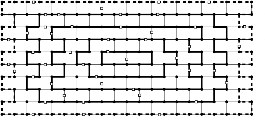
Figure 2: A subdivided wall of height $9$. The white squares represent the subdivision vertices. The bold curves are its layers and the bold-dashed curve is its perimeter.

Given a graph $G$ we denote by ${\bf gw}(G)$ the maximum integer $h$ for which $G$ contains a subdivided wall of height $h$ as a subgraph. The next lemma follows easily by combining results in [22], [26], and [32].

Lemma 2.1.

If $G$ is a planar graph, then ${\bf tw}(G)\leq 9\cdot{\bf gw}(G)+1$.

3 Vital cyclic linkages

Tight concentric cycles.

Let $G$ be a graph embedded in the sphere $\mathbb{S}_{0}$. A sequence ${\cal C}=\{C_{1},\ldots,C_{r}\}$ of concentric cycles of $G$ is tight in $G,$ if

• ${C_{1}}$ is surface minimal, i.e., there is no closed disk $D$ of $\mathbb{S}_{0}$ that is properly contained in $\bar{C_{1}}$ and whose boundary is a cycle of $G$;

• for every $i\in\{1,\ldots,r-1\},$ there is no closed disk $D$ such that $\bar{C}_{i}\subset{D}\subset\bar{C}_{i+1}$ and such that the boundary of $D$ is a cycle of $G$.

See Figure 3 for a an example of the tightness definition.

Figure 3: A sequence of three tight concentric cycles. The addition of any of the dashed edges makes the sequence non-tight.

Graph Linkages.

Let $G$ be a graph. A graph linkage in $G$ is a pair ${\cal L}=(H,T)$ such that $H$ is a subgraph of $G$ without isolated vertices and $T$ is a subset of the vertices of $H,$ called terminals of ${\cal L},$ such that every vertex of $H$ with degree different than 2 is contained in $T$. The set ${\cal P}({\cal L}),$ which we call path set of the graph linkage ${\cal L},$ contains all paths of $H$ whose endpoints are in $T$ and do not have any other vertex in $T$. The pattern of $L$ is the graph

$$(T,\big{\{}\{s,t\}\mid{\cal P}({\cal L})\text{ contains a path from $s$ to $t$ in $H$}\big{\}}).$$

Two graph linkages of $G$ are equivalent if they have the same pattern and are isomorphic if their patterns are isomorphic. A graph linkage ${\cal L}=(H,T)$ is called weakly vital (reps. strongly vital) in $G$ if $V(H)=V(G)$ and there is no other equivalent (resp. isomorphic) graph linkage that is different from ${\cal L}$. Clearly, if a graph linkage ${\cal L}$ is strongly vital then it is also weakly vital. We call a graph linkage ${\cal L}$ linkage if its pattern has maximum degree 1 (i.e., it consists of a collection of paths), in which case we omit $H$ and refer to the linkage just by using ${\cal L}$. We also call a graph linkage ${\cal L}$ cyclic linkage if its pattern is a cycle. For an example of distinct types of cyclic linkages, see Figure 4.

Notice that there is a critical difference between equivalence and isomorphism of linkages. To see this, suppose that ${\cal L}=(C,T)$ is a cyclic linkage of a graph $G$ and let $A_{G}$ be the set of all cyclic linkages that are isomorphic to ${\cal L}$, while $B_{G}$ is the set of all cyclic linkages that are equivalent to ${\cal L}$. Notice that the cycles in the cyclic linkages of $A_{G}$ should meet the terminals in the same cyclic order. On the contrary the cycles of the cyclic linkages of $B_{G}$ may meet the terminals in any possible cyclic ordering. Consequently $A_{G}\subseteq B_{G}$. For example, if ${\cal L}=(C,T)$ is the cyclic linkage of the graphs in Figure 4, then $|A_{G_{1}}|=1$, $|B_{G_{1}}|=1$, $|A_{G_{2}}|=1$, $|B_{G_{2}}|=12$, $|A_{G_{2}}|=4$, $|B_{G_{3}}|=28$.

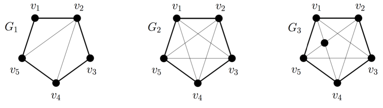
Figure 4: Three graphs $G_{1},G_{2}$, and $G_{3}$. In each graph the bold edges define the cycle $C=(\{v_{1},\ldots,v_{5}\},\{\{v_{1},v_{2}\},\ldots,\{v_{4},v_{5}\},\{v_{5},v_{6}\}\})$ where $T=V(C)$. Consider the cyclic linkage ${\cal L}=\{C,T\}$ where $T=V(C)$. ${\cal L}$ is a weakly vital linkage in $G_{1}$ and $G_{2}$ while it is not a weakly vital linkage in $G_{3}$. Moreover, ${\cal L}$ is a strongly vital linkage in $G_{1}$ while it is not a strongly vital linkage neither in $G_{2}$ nor in $G_{3}$.

CGL-configurations.

Let $G$ be a graph embedded on the sphere $\mathbb{S}_{0}$. Then we say that a pair ${\cal Q}=({\cal C},{\cal L})$ is a CGL-configuration of depth $r$ if $\mathcal{C}=\{C_{1},\ldots,C_{r}\}$ is a sequence of concentric cycles in $G,$ ${\cal L}=(H,T)$ is a graph linkage in $G,$ and $T\cap V(\hat{C}_{r})=\emptyset,$ i.e., all vertices in the terminals of ${\cal L}$ are outside $\bar{C_{r}}$. The penetration of ${\cal L}$ in ${\cal C},$ $p_{\cal C}({\cal L}),$ is the number of cycles of ${\cal C}$ that are intersected by the paths of ${\cal L}$ (when ${\cal L}=(C,S)$ is cyclic we will sometimes refer to the penetration of ${\cal L}$ as the penetration of cycle $C$). We say that ${\cal Q}$ is touch-free if for every path $P\in{\cal L},$ the number of connected components of $P\cap C_{r}$ is not $1$. See figure 5 for an example of a CGL-configuration.

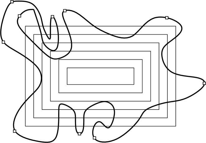
Figure 5: A CLG-configuration ${\cal Q}=({\cal C},{\cal L})$ with ${\cal L}=(H,T)$. Here, ${\cal C}$ is a sequence of six concentric cycles, $H$ (the bold curve) is a cycle (thus ${\cal L}$ is a cyclic linkage) and $T$ is represented by the set of squares. The penetration of ${\cal L}$ in ${\cal C}$ is $4$ and ${\cal Q}$ is touch-free.

Cheap graph linkages.

Let $G$ be a graph embedded on the sphere $\mathbb{S}_{0},$ let ${\cal C}=\{C_{1},\ldots,C_{r}\}$ be a sequence of cycles in $G,$ and let ${\cal L}=(H,T)$ be a graph linkage where $T\subseteq V(G\setminus\hat{C}_{r})$ (notice that $({\cal C},{\cal L})$ is a CGL-configuration). We define function $c$ which maps graph linkages of $G$ to non-negative integers such that

$$c({\cal L})=|E({\cal L})\setminus\bigcup_{i\in\{1,\ldots,r\}}{E(C_{i})}|.$$

A graph linkage ${\cal L}$ of $G$ is $\cal{C}$-strongly cheap (resp. $\cal{C}$-weakly cheap ), if $T({\cal L})\cap\hat{C_{r}}=\emptyset$ and there is no other isomorphic (resp. equivalent) graph linkage ${\cal L}^{\prime}$ such that $c({\cal L})>c({\cal L}^{\prime})$. Obviously, if ${\cal L}$ is ${\cal C}$-strongly cheap then it is also ${\cal C}$-weakly cheap.

Tilted grids.

Let $G$ be a graph. A tilted grid of $G$ is a pair ${\cal U}=({\cal X},{\cal Z})$ where ${\cal X}=\{X_{1},\ldots,X_{r}\}$ and ${\cal Z}=\{Z_{1},\ldots,Z_{r}\}$ are both sequences of $r\geq 2$ vertex-disjoint paths of $G$ such that

• for each $i,j\in\{1,\ldots,r\}$ $I_{i,j}=X_{i}\cap Z_{j}$ is a (possibly edgeless) path of $G,$

• for $i\in\{1,\ldots,r\}$ the subpaths $I_{i,1},I_{i,2},\ldots,I_{i,r}$ appear in this order in $X_{i}$,

• for $j\in\{1,\ldots,r\}$ the subpaths $I_{1,j},I_{2,j},\ldots,I_{r,j}$ appear in this order in $Z_{j}$,

• $E(I_{1,1})=E(I_{1,r})=E(I_{r,1})=E(I_{r,r})=\emptyset,$

• the graph $G_{{\cal U}}^{*}$ taken from the graph $G_{{\cal U}}=(\bigcup_{i\in\{1,\ldots,r\}}X_{i})\cup(\bigcup_{i\in\{1,\ldots,r\}}Z_{i})$ after contracting all edges in $\bigcup_{(i,j)\in\{1,\ldots,r\}^{2}}I_{i,j}$ is isomorphic to the $(r\times r)$-grid.

We refer to the cardinality $r$ of ${\cal X}$ (or ${\cal Z}$) as the capacity of ${\cal U}$.

Tidy tilted grids.

Given a plane graph $G$ and a graph linkage ${\cal L}=(H,T)$ of $G$ we say that a tilted grid ${\cal U}=({\cal X},{\cal Z})$ of $G$ is an ${\cal L}$-tidy tilted grid of $G$ if $T\cap D_{\cal U}=\emptyset$ and $D_{\cal U}\cap{\cal L}=\boldsymbol{\boldsymbol{\cup}}{\cal Z}$ where $D_{\cal U}$ is the closed interior of the perimeter of $G_{\cal U}$ (for an example see Figure 6).

From graph linkages to linkages.

Let $G$ be a graph and let ${\cal L}=(H,T)$ be a graph linkage of $G$. We denote by $G_{\cal L}$ the graph obtained by subdividing all edges of $G$ incident to terminals and then removing the terminals. Similarly, we define ${\cal L}^{*}=(H^{*},T^{*})$ so that $H^{*}$ is the graph obtained by subdividing all edges incident to terminals, removing the terminals, and considering as terminals the subdivision vertices. Notice that ${\cal L}^{*}$ is a linkage of $G_{\cal L}$. Notice that if ${\cal L}$ is strongly vital then ${\cal L}^{*}$ is not necessarily strongly vital. However, if ${\cal L}$ is weakly vital, then so is ${\cal L}^{*}$ (see Figure 6 for an example).

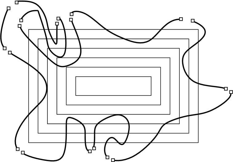
Figure 6: The linkage that corresponds to the cyclic linkage depicted in Figure 5.

Vertex dissolving.

Let $G$ be a graph and $v\in V(G)$ with $N_{G}(v)=\{u,w\}$. The operation of dissolving $v$ in $G$ is the following: Delete $v$ from $G$ and add edge $\{u,w\}$ to $E(G)$, allowing the existence of multiple edges.

The following proposition follows from the combination of Lemma 5, Lemma 6, and Observation 3 of [2].

Proposition 3.1.

Let $G$ be a graph embedded on the sphere $\mathbb{S}_{0}$ and let ${\cal Q}=({\cal C},{\cal L})$ be a touch-free CGL-configuration of $G,$ where ${\cal C}$ is tight in $G$ and ${\cal L}$ is a ${\cal C}$-weakly cheap linkage whose penetration in ${\cal C}$ is at least $r$. Then $G$ contains some ${\cal L}$-tidy tilted grid in $G$ of capacity at least $r/(4\cdot|{\cal P}({\cal L})|)$.

Lemma 3.1.

Let $G$ be a graph embedded on the sphere $\mathbb{S}_{0}$. If $G$ contains a strongly vital cyclic linkage ${\cal L}=(C,T),$ then $G$ does not contain an ${\cal L}$-tidy tilted grid of capacity $4$.

Proof.

Assume that ${\cal L}=(C,T)$ is a strongly vital cyclic linkage in $G$ and that $\Gamma$ is an ${\cal L}$-tidy tilted grid of capacity $4$ in $G$. Let also $\Gamma_{4}$ be the $(4\times 4)$-grid. Observe that $\Gamma_{4}$ is the graph that we get after contracting all edges of $\Gamma$ with at least one endpoint of degree $2$. We contract $\Gamma$ to $\Gamma_{4}$ in $G$ and let $G^{\prime}$ be the resulting graph.
Let $V(\Gamma_{4})=\{v_{ij}\mid i,j\in\{1,\ldots 4\}\}$ and $E(\Gamma_{4})=\{\{v_{ij},v_{i^{\prime}j^{\prime}}\}\mid|i-i^{\prime}|+|j-j^{\prime}|=1\}$. Observe that $\Gamma_{4}$ is also an ${\cal L}$-tidy tilted grid of capacity $4$ in $G^{\prime}$ and that ${\cal L}$ is also strongly vital in $G^{\prime}$ (if not, then it was not strongly vital in $G$). Let $H=\Gamma\cup C$ and $H^{\prime}$ be the contraction of $H$ that we get after contracting all edges of $H$ whose ends have both degree $2$.
Let also $H^{*}=\Gamma_{4}\cup P_{1}\cup P_{2}\cup P_{3}\cup P_{4}$, where for every $i\in\{1,2,3,4\}$, each $P_{i}$ is a path of length $2$ such that $P_{1}$ connects $v_{11}$ with $v_{12}$, $P_{2}$ connects $v_{13}$ with $v_{14}$, $P_{3}$ connects $v_{41}$ with $v_{44}$ and $P_{4}$ connects $v_{42}$ with $v_{43}$ (i.e. for every cyclic linkage ${\cal L}=(C,T)$ if we contract all edges of $H=\Gamma\cup C$ whose ends have degree $2$, we get a graph isomorphic to $H^{*}$ which is a $(4\times 4)$-grid in addition to some paths that are subgraphs of $C$).
It is not hard to confirm that for every possible $H$, its corresponding contraction, $H^{\prime}$, is isomorphic to $H^{*}$. It remains to show that there exists a cyclic linkage ${\cal L^{\prime}}=(C^{\prime},T)$ in $G^{\prime}$, where $C^{\prime}$ is different from $C$. As $H^{*}$ is a unique graph (up to isomorphism), a way of rerouting $C$ (in order to obtain a different cyclic linkage) is given in Figure 7. ∎

Lemma 3.2.

Let $G$ be a graph embedded on the sphere $\mathbb{S}_{0}$ that is the union of $r\geq 2$ concentric cycles ${\cal C}=\{C_{1},\ldots,C_{r}\}$ and one more cycle $C$ of $G$. Assume that ${\cal C}$ is tight in $G,$ $T\cap V(\hat{C}_{r})=\emptyset$, the cyclic linkage ${\cal L}=(C,T)$ is strongly vital in $G$, and its penetration in ${\cal C}$ is $r$. Then $r\leq 16\cdot|T|-1$.

Proof.

Let $\sigma:{\cal P}({\cal L})\rightarrow T$ be such that $\sigma$ is a bijection that maps each path of ${\cal P}({\cal L})$ to one of its endpoints. For every $i\in\{1,\ldots,r\},$ we define ${\cal Q}^{(i)}=({\cal C}^{(i)},{\cal L}^{(i)})$ where ${\cal C}^{(i)}=\{C_{1},\ldots,C_{i}\}$ and ${\cal L}^{(i)}=(C,T^{(i)})$ where

$$T^{(i)}=T\setminus\{\sigma(P)\mid P\in P({\cal L})\mbox{ and }P\cap\hat{C}_{i}=\emptyset\}.$$

Notice that if some ${\cal Q}^{(i+1)}$ is not touch-free, then $T^{(i)}\leq T^{(i+1)}-1$ (as, by the definition of touch-free configurations, there exists at least one path $P$ in ${\cal P}({\cal L})$ such that $P\cap\hat{C}_{i+1}\neq\emptyset$ but $P\cap\hat{C}_{i}=\emptyset$). In the trivial case where every ${\cal Q}^{(i)}$ is not touch-free we derive easily that $r\leq|T|$ and we are done. Otherwise, let ${\cal Q}^{\prime}=({\cal C}^{\prime},{\cal L}^{\prime})$ be the touch-free CGL-configuration in $\{{\cal Q}^{(1)},\ldots,{\cal Q}^{(r)}\}$ of the highest index, say $i$ (as we excluded the trivial case we have that $i\geq 1$). Certainly, ${\cal C}^{\prime}={\cal C}^{(i)}$ and ${\cal Q}^{\prime}$ is tight in $G$. Moreover, ${\cal L}^{\prime}$ is strongly vital in $G$. From Lemma 3.1, $G$ does not contain an ${\cal L}^{\prime}$-tidy tilted grid of capacity $4$. Thus, $G_{\cal L}$ as well does not contain an ${\cal L}^{\prime*}$-tidy (remember how a linkage ${\cal L}^{*}$ is created from a graph linkage ${\cal L}$ after the “duplication” of the terminals of ${\cal L}$) tilted grid of capacity $4$. Recall now that, as ${\cal L}^{\prime}$ is strongly vital in $G$ it is also weakly vital in $G$ and therefore ${\cal L}^{\prime*}$ is weakly vital in ${G}_{{\cal L}^{\prime}}$. Notice also that ${\cal Q}^{\prime*}=({\cal C}^{\prime},{\cal L}^{\prime*})$ is a CGL-configuration of $G_{{\cal L}^{\prime}}$ where ${\cal C}^{\prime}$ is tight in $G_{{\cal L}^{\prime}}$. As ${\cal L}^{\prime*}$ is weakly vital in ${G}_{{\cal L}^{\prime}},$ then, by its uniqueness, ${\cal L}^{\prime*}$ is ${\cal C}^{\prime}$-weakly cheap. Recall that the penetration of ${\cal L}^{\prime}$ in ${\cal C}^{\prime}$ is $r-(i-1)$ and so is the penetration of ${\cal L}^{\prime*}$ in ${\cal C}^{\prime}$. As ${\cal Q}^{\prime},$ and therefore ${\cal Q}^{\prime*}$ as well, is touch-free we can apply Proposition 3.1 and obtain that $G_{{\cal L}^{\prime}}$ contains some ${\cal L}^{\prime*}$-tidy tilted grid of capacity at least $(r-(i-1))/(4\cdot|{\cal P}({\cal L}^{\prime*})|)\leq(r-(i-1))/(4(|{\cal P}({\cal L})|-(i-1))$. We derive that $(r-(i-1))/(4(|{\cal P}({\cal L})|-(i-1))<4,$ therefore $r\leq 16\cdot|{\cal P}({\cal L})|-15(i-1)$ which implies that $r\leq 16\cdot|T|-1$. ∎

Figure 7: On the left, a simplified ${\cal L}$-tidy $(4\times 4)$-grid (corresponding to graph $H^{*}$) and on the right, a rerouting of the cycle of ${\cal L}$ in the grid.

A corollary of Lemma 3.2, with independent combinatorial interest, is the following.

Corollary 3.1.

If a plane graph $G$ contains a strongly vital cyclic linkage ${\cal L}=(C,T),$ then ${\bf tw}(G)=O(|T|^{3/2})$.

Notice that, according to what is claimed in [2], we cannot restate the above corollary for weakly vital linkages, unless we change the bound to be an exponential one. That way, the fact that treewidth is (unavoidably, due to [2]) exponential to the number of terminals for (weakly) vital linkages is caused by the fact that the ordering of the terminals is predetermined.

Lemma 3.3.

Let $G$ be a graph embedded on the sphere $\mathbb{S}_{0}$ that is the union of $r$ concentric cycles ${\cal C}=\{C_{1},\ldots,C_{r}\}$ and a Hamiltonian cycle $C$ of $G$. Let also $T\cap V(\hat{C}_{r})=\emptyset$. If ${\cal L}=(C,T)$ is ${\cal C}$-strongly cheap then ${\cal L}$ is a strongly vital cyclic linkage in $G$.

Proof.

Assume that ${\cal L}$ is not strongly vital in $G,$ i.e., there is a different, isomorphic to ${\cal L}=(C,T),$ cyclic linkage ${{\cal L}^{\prime}}=(C^{\prime},T)$ in $G$. As ${\cal L}\neq{\cal L}^{\prime}$ we have that $C^{\prime}\neq C$, therefore there exists an edge $e\in E(C^{\prime})\setminus E(C)$ (this is because $V(C)=V(C^{\prime})$ which follows from the strong vitality of ${\cal L}$ in $G$).
But, as $E(G)=E(C)\cup\bigcup_{i=1}^{r}E(C_{i}),$ we derive that $e\in\bigcup_{i=1}^{r}E(C_{i})$ (observe that the only way $C^{\prime}$ can be different from $C$ is by using extra edges from the cycles of ${\cal C}$).
Thus, $|E(C^{\prime})\cap\bigcup_{i=1}^{r}E(C_{i})|>|E(C)\cap\bigcup_{i=1}^{r}E(C_{i})|$ and, by the definition of cheap graph linkages, $c({\cal L})>c({\cal L}^{\prime}),$ which contradicts the assumption that ${\cal L}$ is ${\cal C}$-strongly cheap. Therefore, ${\cal L}=(C,T)$ is a strongly vital cyclic linkage in $G,$ as claimed. ∎

We are now able to prove the main combinatorial result of this paper.

Lemma 3.4.

Let $G$ be a plane graph containing some sequence of concentric cycles $\mathcal{C}=\{C_{1},\ldots,C_{r}\}$. Let also ${\cal L}=(C,T)$ be a cyclic linkage of $G$ where $T\cap V(\hat{C}_{r})=\emptyset$. If ${\cal L}$ is ${\cal C}$-strongly cheap then the penetration of ${\cal L}$ in ${\cal C}$ is at most $r\leq 16\cdot|T|-1$.

Proof.

Suppose that some path $P\in{\cal P}({\cal L})$ intersects at least $16\cdot|T|$ cycles of ${\cal C}$. Then, $P$ intersects all cycles in ${\cal C}^{*}=\{C_{r-16\cdot|T|+1},\ldots,C_{r}\}$.
Let $G^{\prime}$ be the graph obtained by $C\cup\boldsymbol{\boldsymbol{\cup}}{\cal C}^{*}$ after dissolving all vertices of degree $2$ that do not belong to $T$ and let ${\cal L}^{\prime}=(C^{\prime},T)$ be the linkage of $G^{\prime}$ obtained from ${\cal L}$ if we dissolve the same vertices in the paths of ${\cal L}$. Similarly, by dissolving vertices of degree 2 in the cycles of ${\cal C}^{*}$ we obtain a new sequence of concentric cycles which, for notational convenience, we denote by $\mathcal{C}^{\prime}=\{C_{1},\ldots,C_{r^{\prime}}\},$ where $r^{\prime}=16\cdot|T|$.
The cyclic linkage ${\cal L}^{\prime}$ is ${\cal C}^{\prime}$-strongly cheap because ${\cal L}$ is ${\cal C}$-strongy cheap (it is easy to observe that no edge of $\bigcup_{i=1}^{r}E(C_{r})\setminus E(C)$ belongs to $E(C^{\prime})$). Notice that $C^{\prime}$ is a Hamiltonian cycle of $G^{\prime}$ and, from Lemma 3.3, ${\cal L}^{\prime}$ is a strongly vital cyclic linkage of $G^{\prime}$. We also assume that ${\cal C}^{\prime}$ is tight (otherwise we can replace it by a tight one and observe that, by its uniqueness, ${\cal L}^{\prime}$ will be cheap to this new one as well). As ${\cal L}^{\prime}$ is ${\cal C}^{\prime}$-strongly cheap and ${\cal C}^{\prime}$ is tight, from Lemma 3.2, $r^{\prime}\leq 16\cdot|T|-1$; a contradiction. ∎

4 The algorithm

This section is devoted to the proof of Theorem 1.2. We consider the following, slightly more general, problem.

Planar Annotated Cyclability
Input: A plane graph $G,$ a set $R\subseteq V(G),$ and a non-negative integer $k$.
Question: Does there exist, for every set $S$ of $k$ vertices in $R,$ a cycle $C$ of $G$ such that $S\subseteq V(C)$?

In this section, for simplicity, we refer to Planar Annotated Cyclability as problem PAC. Theorem 1.2 follows directly from the following lemma.

Lemma 4.1.

There is an algorithm that solves PAC in $2^{2^{O(k^{2}\log k)}}\cdot n^{2}$ steps.

The rest of this section is devoted to the proof of Lemma 4.1.

Problem/color-irrelevant vertices.

Let $(G,k,R)$ be an instance of PAC. We call a vertex $v\in V(G)\setminus R$ problem-irrelevant if $(G,k,R)$ is a yes-instance if and only if $(G\setminus v,k,R)$ is a yes-instance. We call a vertex $v\in R$ color-irrelevant when $(G,k,R)$ is a yes-instance if and only if $(G,k,R\setminus\{v\})$ is a yes-instance.

Before we present the algorithm of Lemma 4.1, we need to introduce three algorithms that are used in it as subroutines.

Algorithm DP$(G,R,k,q,{\cal D})$
Input: A graph $G,$ a vertex set $R\subseteq V(G),$ two non-negative integers $k$ and $q,$ where $k\leq q,$ and a tree decomposition ${\cal D}$ of $G$ of width $q$.
Output: An answer whether $(G,R,k)$ is a yes-instance of PAC or not.
Running time: $2^{2^{O(q\cdot\log q)}}\cdot n$.

Algorithm DP is based on dynamic programming on tree decompositions of graphs. The technical details are presented in Section 5.

Algorithm Compass$(G,q)$
Input: A planar graph $G$ and a non-negative integer $q.$
Output: Either a tree decomposition of $G$ of width at most $18q$ or a subdivided wall $W$ of $G$ of height $q$ and a tree decomposition ${\cal D}$ of the compass $K_{W}$ of $W$ of width at most $18q$.
Running time: $2^{q^{O(1)}}\cdot n$.

We describe algorithm Compass in Subsection 4.1.

Algorithm concentric_cycles$(G,R,k,q,W)$
Input: A planar graph $G,$ a set $R\subseteq V(G),$ a non-negative integer $k,$ and a subdivided wall $W$ of $G$ of height at least $392k^{2}+40k$.
Output: Either a problem-irrelevant vertex $v$ or a sequence ${\cal C}=\{C_{1},C_{2},\ldots,C_{98k+2}\}$ of concentric cycles of $G,$ with the following properties:

1. $\bar{C}_{1}\cap R\neq\emptyset$.

2. The set $R$ is $32k$-dense in ${\cal C}$.

3. There exists a sequence ${\cal W}$ of $2k+1$ paths in $K_{W}$ such that $({\cal C},{\cal W})$ is a $(98k+2,2k+1)$-railed annulus.

Running time: $O(n)$.

We describe Algorithm concentric_cycles in Subsection 4.2. We now use the above three algorithms to describe the main algorithm of this paper which is the following.

Algorithm Planar_Annotated_Cyclability$(G,R,k)$
Input: A planar graph $G,$ a set $R\subseteq V(G),$ and a non-negative integer $k$.
Output: An answer whether $(G,R,k)$ is a yes-instance of PAC or not.
Running time: $2^{2^{O(k^{2}\log k)}}\cdot n^{2}$.

• [Step 1.] Let $r=98k^{2}+2k,$ $y=16k,$ and $q=2y+4r$. If Compass($G,q)$ returns a tree decomposition of $G$ of width $w=18q,$ then return DP$(G,R,k,w)$ and stop. Otherwise, the algorithm Compass($G,q)$ returns a subdivided wall $W$ of $G$ of height $q$ and a tree decomposition ${\cal D}$ of the compass $K_{W}$ of $W$ of width at most $w$.

• [Step 2.] If the algorithm concentric_cycles$(G,R,k,q,W)$ returns a problem-irrelevant vertex $v,$ then return Planar_Annotated_Cyclability$(G\setminus v,R\setminus v,k)$ and stop. Otherwise, it returns a sequence ${\cal C}=\{C_{1},C_{2},\ldots,C_{r}\}$ of concentric cycles of $G$ with the properties (1)–(3).
  

• [Step 3.] For every $i\in\{1,\ldots,r-98k-2\}$ let $w_{i}$ be a vertex in $\hat{A}_{i+k,i+33\cdot k}\cap R$ (this vertex exists as, from property (2), $R$ is $32k$-dense in ${\cal C}$), let $R_{i}=(R\cap V(\hat{C}_{i}))\cup\{w_{i}\},$ and let ${\cal D}_{i}$ be a tree decomposition of $\hat{C}_{i}$ of width at most $w$ – this tree decomposition can be constructed in linear time from ${\cal D}$ as each $\hat{C}_{i}$ is a subgraph of $K_{W}$.

• [Step 4.] If, for some $i\in\{1,\ldots,r-98k-2\},$ the algorithm ${\bf DP}(\hat{C}_{i},R_{i},k,q,{\cal D}_{i})$ returns a negative answer, then return a negative answer and stop. Otherwise return Planar_Annotated_Cyclability$(G,R\setminus v,k)$ where $v\in V(\hat{C_{1}})\cap R$ (the choice of $v$ is possible due to property (1)).

Proof of Lemma 4.1. The only non-trivial step in the above algorithm is Step 4. Its correctness follows from Lemma 4.5, presented in Subsection 4.3.

We now proceed to the analysis of the running time of the algorithm. Observe first that the call of Compass($G,q)$ in Step 1 takes $2^{k^{O(1)}}\cdot n$ steps and, in the case that a tree decomposition is returned, the ${\bf DP}$ requires $2^{2^{O(k^{2}\log k)}}\cdot n$ steps. For Step 2, the algorithm concentric_cycles takes $O(n)$ steps and if it returns a problem-irrelevant vertex, then the whole algorithm is applied again for a graph with one vertex less. Suppose now that Step 2 returns a sequence ${\cal C}$ of concentric cycles of $G$ with the properties (1)–(3). Then the algorithm ${\bf DP}$ is called $O(k^{2})$ times and this takes in total $2^{2^{O(k^{2}\log k)}}\cdot n$ steps. After that, the algorithm either concludes to a negative answer or is called again with one vertex less in the set $R$. In both cases where the algorithm is called again we have that the quantity $|V(G)|+|R|$ is becoming smaller. This means that the recursive calls of the algorithm cannot be more than $2n$. Therefore the total running time is bounded by $2^{2^{O(k^{2}\log k)}}\cdot n^{2}$ as required.

4.1 The algorithm Compass

Before we start the description of algorithm Compass we present a result that follows from Proposition 2.1, the algorithms in [29] and [4], and the fact that finding a subdivision of a planar $k$-vertex graph $H$ that has maximum degree 3 in a graph $G$ can be done, using dynamic programming, in $2^{O(k\cdot\log k)}\cdot n$ steps (see also [1]).

Lemma 4.2.

There exists an algorithm $A_{1}$ that, given a graph $G$ and an integer $h,$ outputs either a tree decomposition of $G$ of width at most $9h$ or a subdivided wall of $G$ of height $h$. This algorithm runs in $2^{h^{O(1)}}\cdot n$ steps.

Description of algorithm Compass

We use a routine, call it $A_{2}$, that receives as input a subdivided wall $W$ of $G$ with height equal to some even number $h$ and outputs a subdivided wall $W^{\prime}$ of $G$ such that $W^{\prime}$ has height $h/2$ and $|V(K_{W^{\prime}})|\leq|V(G)|/4$. $A_{2}$ uses the fact that, in $W,$ there are 4 vertex-disjoint subdivided subwalls of $W$ of height $h/2$. Among them, $A_{2}$ outputs the one with the minimum number of vertices and this can be done in $O(n)$ steps. The algorithm Compass uses as subroutines the routine $A_{2}$ and the algorithm $A_{1}$ of Lemma 4.1.

Algorithm Compass$(G,q)$
[Step 1.]	if	$A_{1}(G,2q)$ outputs a tree decomposition ${\cal D}$ of $G$ with
		width at most $18q$ then return ${\cal D},$
		otherwise it outputs a subdivided wall $W$ of $G$ of height $2q$
[Step 2.]	Let $W^{\prime}=A_{2}(W)$
		if	$A_{1}(K_{W^{\prime}},2q)$ outputs a tree decomposition ${\cal D}$ of
			$K_{W^{\prime}}$ of width at most $18q$ then return $W^{\prime}$ and ${\cal D},$
			otherwise $W\leftarrow{W^{\prime}}$ and go to Step 2.

Notice that, if $A$ terminates after the first execution of Step 1, then it outputs a tree decomposition of $G$ of width at most $18q$. Otherwise, the output is a subdivided wall $W^{\prime}$ of height $q$ in $G$ and a tree decomposition of $K_{W^{\prime}}$ of width at most $18q$ (notice that as long as this is not the case, the algorithm keeps returning to step 2). The application of routine $A_{2}$ ensures that the number of vertices of every new $K_{W}$ is at least four times smaller than the one of the previous one. Therefore, the $i$-th call of the algorithm $A_{1}$ requires $O(2^{h^{O(1)}}\cdot\frac{n}{2^{2(i-1)}})$ steps. As $\sum_{i=0}^{\infty}\frac{1}{2^{2i}}=O(1),$ algorithm Compass has the same running time as algorithm $A_{1}$.

4.2 The Algorithm concentric_cycles

We need to introduce two lemmata. The first one is strongly based on the combinatorial Lemma 3.4 that is the main result of Section 3.

Lemma 4.3.

Let $(G,R,k)$ be an instance of PAC and let ${\cal C}=\{C_{1},\ldots,C_{r}\}$ be a sequence of concentric cycles in $G$ such that $V(\hat{C}_{r})\cap R=\emptyset$. If $r\geq 16\cdot k,$ then all vertices in $V(\hat{C}_{1})$ are problem-irrelevant.

Proof.

We observe that for every vertex $v\in V(G),$ if $(G\setminus v,R,k)\in\Pi$ then $(G,R,k)\in\Pi$ because $G\setminus v$ is a subgraph of $G$ and thus every cycle that exists in $G\setminus v$ also exists in $G$.
Assume now that $(G,R,k)\in\Pi,$ let $v\in V(\hat{C}_{1}),$ and let $S\subseteq R,$ $|S|\leq k$. We will prove that there exists a cycle in $G\setminus v$ containing all vertices of $S$.
As $(G,R,k)\in\Pi,$ there is a cyclic linkage ${\cal L}=(C,S)$ in $G$. If $v\notin V(C),$ then $C$ is a subgraph of $G\setminus v$ and we are done. Else, if $v\in V(C),$ let ${\cal L}^{\prime}=(C^{\prime},S)$ be a ${\cal C}$-weakly cheap cyclic linkage in the graph $H=G[V(C)\cup\bigl{(}\bigcup_{i=1}^{r}V(C_{i})\bigr{)}],$ and assume that $v\in V(C^{\prime})$ too. Then $C^{\prime}$ meets all cycles of ${\cal C}$ and its penetration in ${\cal C}$ is more than $16\cdot|S|,$ which contradicts Lemma 3.4.
Thus, $v\notin V(C^{\prime})$ implying that there exists a cyclic linkage with $S$ as its set of terminals that does not contain $v$. As $S$ was arbitrarily chosen, vertex $v$ is problem-irrelevant. ∎

Lemma 4.4.

Let $y,r,q,z$ be positive integers such that $y+1\leq z\leq r,$ $G$ be a graph embedded on $\mathbb{S}_{0}$ and let $R\subseteq V(G)$ be the set of annotated vertices of $G$. Given a subdivided wall $W$ of height $h=2\cdot\max\{y,\lceil\frac{q}{8}\rceil\}+4r$ in $G$ then either $G$ contains a sequence ${\cal C}^{\prime}=\{C^{\prime}_{1},C^{\prime}_{2},\ldots,C^{\prime}_{y}\}$ of concentric cycles such that $V(\hat{C}^{\prime}_{y})\cap R=\emptyset$ or a sequence ${\cal C}=\{C_{1},C_{2},\ldots,C_{r}\}$ of concentric cycles such that:

1. $\bar{C}_{1}\cap R\neq\emptyset$.

2. $R$ is $z$-dense in ${\cal C}$.

3. There exists a collection ${\cal W}$ of $q$ paths in $K_{W},$ such that $({\cal C},{\cal W})$ is a $(r,q)$-railed annulus in $G$.

Moreover, a sequence ${\cal C}^{\prime}$ or ${\cal C}$ of concentric cycles as above can be constructed in $O(n)$ steps.

Proof.

Let $p=\max\{y,\lceil\frac{q}{8}\rceil\}$. We are given a subdivided wall $W$ of height $h=2p+4r$ and we define ${\cal C}=\{C_{1},\ldots,C_{r}\}$ such that $C_{i}=J_{\frac{h}{2}-p-2i+2},i\in\{1,\ldots,r\}$. Notice that there is a collection ${\cal W}$ of $8p$ vertex disjoint paths in $W$ such that $({\cal C},{\cal W})$ is a $(r,q)$-railed annulus. If $\bar{C}_{1}\cap R=\emptyset,$ then ${\cal C}^{\prime}=\{J_{\frac{h}{2}},\ldots,J_{\frac{h}{2}+y-1}\}$ is a sequence of concentric cycles where $\bar{J}_{\frac{h}{2}+y-1}\subseteq\mathring{C_{1}}$ and we are done. Otherwise, we have that ${\cal C}$ satisfies property 1.
Suppose now that Property 2 does not hold for ${\cal C}$. Then, there exists some $i\in\{1,\ldots,r\}$ such that $A_{i,i+z-1}\cap R=\emptyset$. Notice that $A_{i,i+z-1}$ contains $2z-1>2y$ layers of $W$ which are crossed by at least $2y$ of the paths in ${\cal W}$ (these paths certainly exist as $2y<8p$). This implies the existence of a wall of height $2y$ in $A_{i,i+z-1}$ which, in turn contains a sequence ${\cal C}^{\prime}=\{C_{1}^{\prime},\ldots,C_{y}^{\prime}\}$ of concentric cycles. As $\bar{C}_{y}^{\prime}\subseteq A_{i,i+z-1}$ we have that $V(\hat{C}^{\prime}_{y})\cap R=\emptyset$ and we are done. It remains to verify property 3 for ${\cal C}$. This follows directly by including in ${\cal W}^{\prime}$ any $q\leq 8p$ of the disjoint paths of ${\cal W}$. Then $({\cal C},{\cal W}^{\prime})$ is the required $(r,q)$-railed annulus. It is easy to verify that all steps of this proof can be turned to an algorithm that runs in linear, on $n,$ number of steps. ∎

Description of algorithm concentric_cycles

This algorithm first applies the algorithm of Lemma 4.4 for $y=16k,$ $r=98k^{2}+2k,$ $q=2k+1,$ and $z=32k$. If the output is a sequence ${\cal C}^{\prime}=\{C^{\prime}_{1},C^{\prime}_{2},\ldots,C^{\prime}_{y}\}$ of concentric cycles such that $V(\hat{C}^{\prime}_{y})\cap R=\emptyset$, then it returns a vertex $w$ of $\hat{C}_{1}^{\prime}$. As $V(\hat{C}_{r})\cap R=\emptyset,$ Lemma 4.3 implies that $w$ is problem-irrelevant. If the output is a sequence ${\cal C}$ the it remains to observe that conditions 1–3 match the specifications of algorithm concentric_cycles.

4.3 Correctness of algorithm Planar_Annotated_Cyclability

As mentioned in the proof of Lemma 4.1, the main step – [step 4] – of algorithm Planar_Annotated_Cyclability is based on Lemma 4.5 below.

Lemma 4.5.

Let $(G,R,k)$ be an instance of problem PAC and let $b=98k+2$ and $r=98k^{2}+2k$. Let also $({\cal C},{\cal W})$ be a $(r,2k+1)$-railed annulus in $G,$ where ${\cal C}=\{C_{1},\ldots C_{r}\}$ is a sequence of concentric cycles such that $\hat{C}_{1}$ contains some vertex $v\in R$ and that $R$ is $32k$-dense in ${\cal C}$. For every $i\in\{1,\ldots,r-b\}$ let $R_{i}=(R\cap V(\hat{C}_{i}))\cup\{w_{i}\},$ where $w_{i}\in V(\hat{A}_{i+k+1,33k+i+1})\cap R$. If $(\hat{C}_{i+b},R_{i},k)$ is a no-instance of ${\rm\Pi},$ for some $i\in\{1,\ldots,r-b\},$ then $(G,R,k)$ is a no-instance of PAC. Otherwise vertex $v$ is color-irrelevant.

We first prove the following lemma, which reflects the use of the rails of a railed annulus and is crucial for the proof of Lemma 4.5.

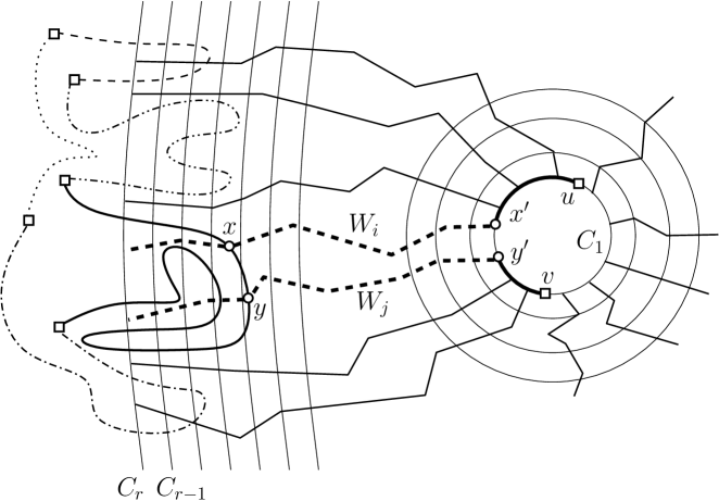
Figure 8: Visualization of proof of Lemma 4.6, case 1. The different lining on the parts of the cycle at the left indicates the different colors of these paths.

Lemma 4.6.

Let $G$ be a graph embedded on the sphere $\mathbb{S}_{0},$ $r,k$ be two positive integers such that $r\geq 16k$, and $({\cal C},{\cal W})$ be an $(r,2k+1)$-railed annulus of $G$ with ${\cal C}=\{C_{1},\ldots,C_{r}\}$ being its sequence of concentric cycles, ${\cal W}=\{W_{1},\ldots,W_{2k+1}\}$ its rails. Let also $S\subseteq V(G)$ such that $S\cap\hat{C}_{r}=\emptyset$ and $|S|=k$. Then for every two vertices $u,v\in V(C_{1}),$ if there exists a cyclic linkage ${\cal L}=(C,S),$ with penetration $k+1\leq p_{\cal C}({\cal L})\leq r-1,$ in $G,$ then there exists a path $P_{u,v}$ with ends $u$ and $v$ that meets all vertices of $S$.

Proof.

Let $\{s_{1},\ldots,s_{k}\}$ be an ordering of the set $S$ and let $f_{\cal L}:{\cal L}({\cal P})\rightarrow\{1,\ldots,k\}$ be a function such that for every $i\in\{1,\ldots k-1\}$, $f_{\cal L}(P)=i$ if the endpoints of $P$ are $s_{i}$ and $s_{i+1}$ and $f_{\cal L}(P^{*})=k$ for the unique path $P^{*}\in{\cal P}({\cal L})$ whose endpoints are $s_{k}$ and $s_{1}$.
Moreover, as $W_{i}$ is a path with endpoints $w^{\prime}_{i}\in V(C_{1})$ and $w^{\prime\prime}_{i}\in V(C_{r}),$ we define the ordering $\{w^{\prime}_{i},\ldots,w^{\prime\prime}_{i}\}$ of $V(W_{i})$ and call it the natural ordering of $W_{i}$. Furthermore, for every $W_{i}\in{\cal W},$ let $m_{\cal L}(W_{i})=f_{\cal L}(P)$ if $P$ is the first path (with respect to the natural ordering of $W_{i}$) of ${\cal P}({\cal L})$ that $W_{i}$ meets and $m_{\cal L}(W_{i})=0$ if $W_{i}$ does not meet $C$.
Let $C_{j}\in{\cal C}$. We pick an arbitrary vertex $v_{1}^{j}\in V(C_{j})$ and order $V(C_{j})$ starting from $v_{1}^{j}$ and continuing in clockwise order. Let $\{v_{1}^{j},\ldots,v_{|V(C_{j})|}^{j}\}$ be such an ordering of the vertices of $C_{j}$. We assign to each vertex of $v_{i}^{j}\in C_{j}$ a “color” from the set $\{0,\ldots k\}$ as follows: $c_{\cal L}(v_{i}^{j})=0$ if $v_{i}^{j}\notin V(C_{j})\cap V(C)$ and $c_{\cal L}(v_{i}^{j})=f_{\cal L}(P)$ if $v_{i}^{j}\in V(C_{j})\cap V(P),$ where $P\in{\cal P}({\cal L})$.
For the rest of the proof, if $P_{0}$ is a path, $P_{0}(v,w)$ is the subpath of $P_{0}$ with endpoints $v$ and $w$. We examine two cases:

1. At least $k+1$ paths of ${\cal W}$ (i.e. rails of the railed annulus) meet $C$. Then, as $|{\cal P}({\cal L})|=k,$ there exist two rails $W_{i},W_{j}\in{\cal W}$ and a path $P\in{\cal P}({\cal L})$ such that $m_{\cal L}(W_{i})=m_{\cal L}(W_{j})=f_{\cal L}(P)$. Let $V(C_{1})\cap V(W_{i})$ be the vertices of path $Q_{1,i}$ and $V(C_{1})\cap V(W_{j})$ the vertices of path $Q_{1,j}$. Then, we let $x\in V(C_{1})$ be the endpoint of $Q_{1,i}$ that is not $w^{\prime}_{i}$ and $y\in V(C_{1})$ be the endpoint of $Q_{1,j}$ that is not $w^{\prime}_{j}$ (notice that $x$ and $y$ can coincide with $u$ and $v$). Let also $x^{\prime}$ be the vertex of $V(P)\cap V(W_{i})$ with the least index in the natural ordering of $W_{i}$ and $y^{\prime}$ be the vertex of $V(P)\cap V(W_{j})$ with the least index in the natural ordering of $W_{j}$. We observe that there exist two vertex disjoint paths $P_{1}$ and $P_{2}$ with endpoints either $v,x$ and $u,y$ or $v,y$ and $u,x,$ respectively. We define path $P_{u,v}=(C\setminus P(x^{\prime},y^{\prime}))\cup W_{i}(x,x^{\prime})\cup W_{j}(y,y^{\prime})\cup P_{1}\cup P_{2}$. Path $P_{u,v}$ has the desired properties. See also Figure 8.

2. There exist $k^{\prime}=k+1$ paths, say ${\cal W}^{\prime}=\{W_{1},\ldots,W_{k^{\prime}}\},$ of ${\cal W}$ that do not meet $C$. As the penetration of $C$ is at least $k+1,$ for every $j\in\{r-k,\ldots,r\},$ $V(C_{j}\cap C)\neq\emptyset$. For every $i\in\{1,\ldots,k^{\prime}\}$ and every $j\in\{r-k,\ldots,r\}$ we assign to the vertex $w_{i}^{j}$ of $V(W_{i}\cap C_{j})$ with the least index in the natural ordering of $W_{i},$ a “color” from the set $\{1,\ldots,k\}$ as follows: $c_{\cal L}(w_{i}^{j})=c_{\cal L}(v)$ if there exists a $v\in V(C)$ and a subpath $C_{j}(w_{i}^{j},v)$ (starting from $w_{i}^{j}$ and following $C_{j}$ in counter-clockwise order) such that it does not contain any other vertices of $V(C)$ as internal vertices. For every $W_{i}\in{\cal W}^{\prime},$ we assign to $W_{i}$ a set of colors, ${\chi}_{i}=\bigcup_{j=1}^{k+1}c_{\cal L}(w_{i}^{j})$. Let ${\cal P}$ be the set of all maximal paths of $C_{r}$ without internal vertices in $C$. Certainly, any $W_{i}\in{\cal W}^{\prime}$ intersects exactly one path of ${\cal P}$. We define the equivalence relation $\sim$ on the set of rails ${\cal W}^{\prime}$ as follows: $W_{i}\sim W_{l}$ if and only if $W_{i}$ and $W_{l}$ intersect the same path of ${\cal P}$. We distinguish two subcases:

   • The number of equivalence classes of $\sim$ is $k^{\prime}$. Then, there exist two rails $W_{i},W_{l}\in{\cal W}^{\prime}$ and $j_{i},j_{l}\in\{r-k,\ldots,r\}$ such that $c_{\cal L}(w_{i}^{j_{i}})=c_{\cal L}(w_{l}^{j_{i}})=c_{\cal L}(P)$ for some path $P\in{\cal P}({\cal L})$.

   • The number of equivalence classes of $\sim$ is strictly less than $k^{\prime}$. Then, there exist two rails $W_{i},W_{l}\in{\cal W}^{\prime}$ such that $c_{\cal L}(w_{i}^{j})=c_{\cal L}(w_{l}^{j})$ for every $j\in\{r-k,\ldots,r\}$. Therefore, there exist $j_{i},j_{l}\in\{r-k,\ldots,r\}$ with $j_{i}\neq j_{l}$ such that $c_{\cal L}(w_{i}^{j_{i}})=c_{\cal L}(w_{l}^{j_{l}})=c_{\cal L}(P)$ for some path $P\in{\cal P}({\cal L})$ (this holds because $|\{r-k,\ldots,r\}|=k+1$ – see also Figure 9).

   For both subcases, as $c_{\cal L}(w_{i}^{j_{i}})=c_{\cal L}(P),$ there exist a $v_{j}\in V(P)$ and a subpath $C_{j}(w_{i}^{j_{i}},v_{j})$ of $C_{j}$ and, similarly, as $c_{\cal L}(w_{l}^{j_{l}})=c_{\cal L}(P),$ there exist a $v_{j_{l}}\in V(P)$ and a subpath $C_{j}(w_{l}^{j_{l}},v_{j_{l}})$ of $C_{j}$. These two subpaths do not contain any other vertices of $C$ apart from $v_{j_{i}}$ and $v_{j_{l}},$ respectively. Moreover, let $x$ be the vertex of $V(W_{i}\cap C_{1})$ of the least index in the natural ordering of $W_{i}$ and $y$ the vertex of $V(W_{l}\cap C_{1})$ of the least index in the natural ordering of $W_{l}$. As in case 1, observe that there exist two vertex disjoint paths $P_{1}$ and $P_{2}$ with endpoints either $v,x$ and $u,y$ or $v,y$ and $u,x,$ respectively. We define path $P_{u,v}=(C\setminus P(v_{j_{i}},v_{j_{l}}))\cup C_{j}(w_{i}^{j_{i}},v_{j_{i}})\cup C_{j}(w_{l}^{j_{l}},v_{j_{l}})\cup W_{i}(w_{i}^{j_{i}},x)\cup W_{l}(w_{l}^{j_{l}},y)\cup P_{1}\cup P_{2}$. Path $P_{u,v}$ has the desired properties

∎

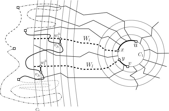
Figure 9: Visualization of proof of Lemma 4.6, case 2, subcase 2.

Proof of Lemma 4.5.

We first prove that if $(\hat{C}_{i+b},R_{i},k)$ is a yes-instance of PAC for every $i\in\{1,\ldots,r-b\},$ then $(G,R,k)$ is a yes-instance of PAC iff $(G,R\setminus v,k)$ is a yes-instance of PAC.
For the non-trivial direction, we assume that $(G,R\setminus v,k)$ is a yes-instance of PAC and we have to prove that $(G,R,k)$ is also a yes-instance of PAC. Let $S\subseteq R$ with $|S|\leq k$. We have to prove that $S$ is cyclable in $G$. We examine two cases:

1. $v\notin S$. As $(G,R\setminus v,k)$ is a yes-instance of ${\rm\Pi},$ clearly there exists a cyclic linkage ${\cal L}=(C,S)$ in $G,$ i.e., $S$ is cyclable in $G$.

2. $v\in S$. As $r\geq k(98k+1)$ and $S\leq k,$ there exists $i$ such that $A_{i,i+98k}\cap S=\emptyset$. We distinguish two sub-cases:

   Subcase 1. $S\subseteq\bar{C}_{i+98k+1}$. Then, as $(\hat{C}_{i+98k+1},R_{i+98k+1},k)$ is a yes-instance of ${\rm\Pi},$ then $S$ is cyclable in $\hat{C}_{i+98k+1}$ and therefore also in $G$.

   Subcase 2. There is a partition $\{S_{1},S_{2}\}$ of $S$ into two non-empty sets, such that $S_{1}\subset\mathring{C_{i}}$ and $S_{1}\cap\bar{C}_{i+98k+1}=\emptyset$. As $R$ is $32k$-dense in ${\cal C},$ there exists a vertex $v_{1}\in S\cap A_{i+k+1,i+33k+1}$ and a vertex $v_{2}\in S\cap A_{50+k+1,i+82k+1}$. For $i\in\{1,2\},$ let $S_{i}^{\prime}=S_{i}\cup\{v_{i}\}$ and observe that $|S_{i}|\leq k$. Let ${\cal C}_{1}=\{C_{i+49k},\ldots,C_{i}\}$ and ${\cal C}_{2}=\{C_{i+49k},\ldots,C_{98k}\}$. As $(\hat{C}_{i+98k+1},R_{98k+1},k)$ is a yes-instance of ${\rm\Pi},$ $S_{1}^{\prime}$ is cyclable in $\hat{C}_{i+98k+1}$. Also, $(G,R\setminus v,k)$ is a yes-instance, $S_{2}^{\prime}$ is cyclable in $G$. For each $i\in\{1,2\},$ there exists a cyclic linkage ${\cal L}_{i}=(C_{i},S_{i}^{\prime})$ that has penetration at least $k+1$ in ${\cal C}_{i}$. We may assume that ${\cal L}_{i}$ is ${\cal C}_{i}$-cheap. Then, By Lemma 4.3, the penetration of ${\cal L}_{i}$ in ${\cal C}_{i}$ is at most $49k$. Let ${\cal L}_{i}^{\prime}=(C_{i},S_{i}),i\in\{1,2\}$. For notational convenience we rename ${\cal C}_{1}$ and ${\cal C}_{2}$ where ${\cal C}_{1}=\{C^{1}_{1},\ldots,C^{1}_{49k+1}\}$ and ${\cal C}_{2}=\{C^{2}_{1},\ldots,C^{2}_{49k+1}\}$ (notice that $C_{49k+1}^{1}=C_{1}^{2}$). Let $x,y$ be two distinct vertices in $C_{i+49k}$. For $i\in\{1,2\},$ we apply Lemma 4.6, for $r=49k+1,$ $k,$ ${\cal C}_{i},$ ${\cal W},$ and $x$ and $y$ and obtain two paths $P_{i},i\in\{1,2\},$ such that $S_{i}\subseteq V(P_{i})$ and whose endpoints are $x$ and $y$. Clearly, $P_{1}\cup P_{2}$ is a cycle whose vertex set contains $S$ as a subset. Therefore $S$ is cyclable in $G,$ as required (see Figure 10).

. ∎

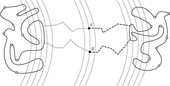
Figure 10: The squares of the right (resp. left) part represent the vertices of $S_{1}$ (resp. $S_{2}$). The connection between two cycles via rails and through $x$ and $y$ is derived from a double application of Lemma 4.6.

5 Dynamic Programming for Planar Cyclability

In this section we present a dynamic programming algorithm for solving Cyclability on graphs of bounded treewidth. We obtain the following algorithm.

Algorithm DP$(G,R,k,q,{\cal D})$
Input: A graph $G,$ a vertex set $R\subseteq V(G),$ two non-negative integers $k$ and $q,$ where $k\leq q,$ and a tree decomposition ${\cal D}$ of $G$ of width $q$.
Output: An answer whether $(G,R,k)$ is a yes-instance of Planar Annotated Cyclability problem, or not.
Running time: $2^{2^{O(q\cdot\log q)}}\cdot n$.

We observe that the question of Planar Annotated Cyclability can be expressed in monadic second-order logic (MSOL). It is sufficient to notice that an instance $(G,R,k)$ is a yes-instance of Planar Annotated Cyclability if and only if for any (not necessarily distinct) $v_{1},\ldots,v_{k}\in R,$ there are sets $X\subseteq V(G)$ and $S\subseteq E(G)$ such that $v_{1},\ldots,v_{k}\in X$ and $C=(X,S)$ is a cycle. The property of $C=(X,S)$ being a cycle is equivalent to asking whether

• for any $x\in X,$ there are two distinct $e_{1},e_{2}\in S$ such that $x$ is incident to $e_{1}$ and $e_{2},$

• for any $x\in X$ and any three pairwise distinct $e_{1},e_{2},e_{3}\in S,$ $e_{1}$ is not incident to $x$ or $e_{2}$ is not incident to $x$ or $e_{3}$ is not incident to $x,$ and

• for any $Z_{1},Z_{2}\subseteq X$ such that $Z_{1}\cap Z_{2}=\emptyset,$ $Z_{1}\neq\emptyset,$ $Z_{2}\neq\emptyset$ and $Z_{1}\cup Z_{2}=X,$ there is $\{x,y\}\in S$ such that $x\in Z_{1}$ and $y\in Z_{2}$.

By the celebrated Courcelle’s theorem (see, e.g., [8, 7]), any problem that can be expressed in MSOL can be solved in linear time for graphs of bounded treewidth.
As we saw, Planar Annotated Cyclability can be solved in $f(q,k)\cdot n$ steps if the treewidth of an input graph is at most $q$, for some computable function $f$.
As the general estimation of $f$ provided by Courcelle’s theorem is immense, we give below a dynamic programming algorithm in order to achieve a more reasonably running time.

First we introduce some notation.

For every two integers $a$ and $b$, with $a<b$, we denote by $\left\llbracket a,b\right\rrbracket$ the set of integers $\{a,a+1,\ldots,b\}$. Let $S$ be a set and $i\in\mathbb{N}$. We define $S^{[i]}=\{A\subseteq S\mid|A|=i\}$.

Sub-cyclic pairs.

Let $G$ be a graph, $C$ a cycle in $G$, and $\{A,X,B\}$ a partition of $V(G)$ such that no edge of $G$ has one endpoint in $A$ and the other in $B$. The restriction of $C$ in $G[A\cup X]$ is called a sub-cyclic pair of $G$ (with respect to $A$, $X$ and $C$). We denote such a sub-cyclic pair by $({\cal Q},Z)$, where ${\cal Q}$ contains the connected components of the restriction of $C$ in $G[A\cup X]$ (observe that ${\cal Q}$ can contain isolated vertices, a unique cycle, and disjoint paths) and $Z=V(C)\cap X$.

Nice tree decompositions.

Let $G$ be a graph. A tree decomposition ${\cal D}=(T,{\cal X})$ of $G$ is called a nice tree decomposition of $G$ if $T$ is rooted to some leaf $r$ and:

1. for any leaf $l\in V(T)$ where $l\neq r$, $X_{l}=\emptyset$ (we call $X_{l}$ leaf node of ${\cal D}$, except from $X_{r}$ which we call root node)

2. the root and any non-leaf $t\in V(T)$ have one or two children

3. if $t$ has two children $t_{1}$ and $t_{2}$, then $X_{t}=X_{t_{1}}=X_{t_{2}}$ and $X_{t}$ is called join node

4. if $t$ has one child $t^{\prime}$, then

   • either $X_{t}=X_{t^{\prime}}\cup\{v\}$ (we call $X_{t}$ insert node and $v$ insert vertex)

   • or $X_{t}=X_{t^{\prime}}\setminus\{v\}$ (we call $X_{t}$ forget node and $v$ forget vertex).

Pairings.

Let $W$ be a set. A pairing of $W$ is an undirected graph $H$ with vertex set $V(H)\subseteq W$ and where each vertex has degree at most 2 (a loop contributes 2 to the degree of its vertex) and if $H$ contains a cycle then this cycle is unique and all vertices not in this cycle have degree 0. Moreover, $H$ may also contain the vertex-less loop. We denote by ${\cal P}(W)$ the set of all pairings of $W$. It is known that if $|W|=w$ then $|{\cal P}(W)|=2^{O(w\cdot\log w)}$.

Edge lifts.

Let $G$ be a graph and $v\in V(G)$ such that $\deg_{G}(v)=2$. Let also $N_{G}(v)=\{u,w\}$. We say that the operation of deleting edges $\{v,u\}$ and $\{v,w\}$ and adding edge $\{u,w\}$ (if it does not exist, i.e. we do not allow double edges) is the edge lift from vertex $v$. We denote by lift$(G,v)$ the graph resulting from $G$ after the edge lift from $v$.
For a vertex set $L\subseteq V(G)$ and a vertex $v\in V(G)$ we say that graph $H$=lift$(G,v)$ is the result of an $L$-edge-lift if $v\in L$.

Let $(G,R,k)$ be an instance of $p$-Annotated Cyclability. Let also ${\cal D}=(T,{\cal X},r)$ be a nice tree decomposition of $G$ of width $w$, where $r$ is the root of $T$. For every $x\in V(T)$ let $T_{t}$ be the subtree of $T$ rooted at $t$ (the vertices of $T_{t}$ are $t$ and its descendants in $T$). Then for every $t\in V(T)$, we define

$$G_{t}=G\Bigl{[}\bigcup_{t^{\prime}\in V(T_{t})}X_{t^{\prime}}\Bigr{]}\mbox{\leavevmode\nobreak\ and\leavevmode\nobreak\ }V_{t}=V(G_{t}).$$

For every $i\in\mathbb{Z}_{>0}$, we set ${\cal R}_{t}^{i}=(V(G_{t})\cap R)^{[i]}$. We also denote ${\cal R}_{t}=\bigcup_{i=1}^{k}{\cal R}_{t}^{i}$.

If $({\cal Q},Z)$ is a sub-cyclic pair of $G_{t}$ where $X_{t}$ is thought of as the separator and $Z\subseteq X_{t}$, we simply say that $({\cal Q},Z)$ is a sub-cyclic pair on $t$. Notice that each sub-cyclic pair $({\cal Q},Z)$ on $t$ corresponds to a pairing in ${\cal P}(X_{t})$, which we denote by $P_{{\cal Q},Z}$ (just dissolve all vertices of ${\cal Q}$ that do not belong to $X_{t}$).

Let $P$ be a pairing of $X_{t}$ and $S$ be a subset of $V(G_{t})$. We say that vertex set $S$ realizes $P$ in $G_{t}$ if there exists a sub-cyclic pair $({\cal Q},Z)$ on $t$ such that $P_{{\cal Q},Z}=P$ and $S\subseteq V(\boldsymbol{\boldsymbol{\cup}}{\cal Q})$.

We also define the signature of $S$ in $G_{t}$ to be the set of all pairings of $X_{t}$ that $S$ realizes and we denote it by ${\bf sig}_{t}(S).$ Notice that ${\bf sig}_{t}(S)\subseteq{\cal P}(X_{t})$, therefore $|{\bf sig}_{t}(S)|=2^{O(w\cdot\log w)}$.

Tables.

We describe the tables of the dynamic programming algorithm. For each $t\in V(T)$, we define ${\cal C}_{t}=\left\llbracket 0,k\right\rrbracket\times X_{t}^{[i]}\times{\cal P}(X_{t})$ and

$${\cal F}_{t} = \{(i,K,{\cal P})\in{\cal C}_{t}\mid\exists S\in{\cal R}_{t}^{i}\text{ such that }K=X_{t}\cap S\mbox{ and }{\bf sig}_{t}(S)={\cal P}\}$$

We call ${\cal F}_{t}$ the table at node $t\in V(T)$. As $|{\cal P}(X_{t})|={2^{O(w\cdot\log w)}}$, it follows that $|{\cal F}(t)|=2^{2^{O(w\cdot\log w)}}$.

Observe that $(G,R,k)$ is a yes-instance of $p$-Annotated Cyclability if and only if ${\cal F}_{r}=\{(0,\emptyset,P_{r}),(1,\emptyset,P_{r}),\ldots,(k,\emptyset,P_{r})\}$, where $P_{r}$ is the unique pairing of ${\cal P}(X_{r})$, i.e., the pairing that is the vertex-less loop (i.e., contains no vertices and a single edge with no endpoints).

New pairings from old.

Before we describe the dynamic programming algorithm we need some definitions. Suppose that $t$ is an insert node of ${\cal D}$ and $X_{t}=X_{s}\cup\{v\}$, where $s$ is the only child of $t$ in $T$ and $v\in V(G)$. Let $E_{v}^{t}=\{\{v,u\}\in E\mid u\in X_{t}\}$. We denote by ${\cal P}_{v}^{\rm aux}$ the set of all graphs $(V,E)$ where $V\subseteq N_{G_{t}}(v)\cup\{v\}$ and $E\subseteq E_{v}^{t}$. For any $P\in{\cal P}(X_{s})$, $\widetilde{P}\in{\cal P}_{v}^{\rm aux}$, and $L\subseteq X_{t}$, we define:

$$P\oplus_{L}\widetilde{P}=\{P^{\prime}\in{\cal P}(X_{t})\mid P\text{ results from }P\cup\widetilde{P}\text{ after a sequence of $L$-edge-lifts}\}.$$

Figure 11: At the top we depict the neighborhood of node $v$ in $X_{s}$ (at the left) and an element, $\tilde{P}$ of $P_{v}^{aux}$ at the right. In the middle we depict the result, $Q$, of the union $P\cup\tilde{P}$, where $P\in{\cal P}(X_{s})$. At the bottom we have the result, $P^{\prime}\in{\cal P}(X_{s}\cup\{v\})={\cal P}(X_{t})$, of lifting $v$ in $Q$.

See Figure 11 for a visualization of the above definitions. For every $P^{\prime}\in{\cal P}(X_{t})$ and $L\subseteq X_{t}$, we define

$$\zeta_{L}(P^{\prime})=\{P\in{\cal P}(X_{s})\mid\exists\widetilde{P}\in{\cal P}_{v}^{\rm aux}\text{ such that }P^{\prime}\in{P\oplus_{L}\widetilde{P}}\}$$

We are now ready to describe the dynamic programming algorithm. We distinguish the following cases for the computation of ${\bf table}(t)$, $t\in V(G)$:

Node $t$ is a leaf node:

​ as $X_{t}=\emptyset$, we have that ${\cal F}(t)=\{(0,\emptyset,G_{\emptyset})\}$ where $G_{\emptyset}$ is the void graph.

Node $t$ is an insert node:

Let $X_{t}=X_{s}\cup\{v\}$, where $s$ is the unique child of $t$ in $T$. We construct ${\bf table}(t)$ by using the following procedure:

Procedure make_join
Input: a subset ${\cal A}$ of ${\cal C}_{s}$
Output: a subset ${\cal B}$ of ${\cal C}_{t}$
let ${\cal B}=\emptyset$
for	$(i,K,{\cal P})\in{\cal A}$
	if	$v\in R$ and $i<k$ then
		let	${\cal B}={\cal B}\cup\{(i+1,K\cup\{v\},{\cal P}^{\prime})\}$
			where ${\cal P}^{\prime}=\{P\in{\cal P}(X_{t})\mid\zeta_{X_{s}\setminus K}(P)\cap{\cal P}\neq\emptyset\}$
	let	${\cal B}={\cal B}\cup\{(i,K,{\cal P}^{\prime\prime})\}$
			where ${\cal P}^{\prime\prime}=\{P\in{\cal P}(X_{t})\mid\zeta_{X_{t}\setminus K}(P)\cap{\cal P}\neq\emptyset\}$

Lemma 5.1.

${\cal F}_{t}=\mbox{\bf make\_join}({\cal F}_{s})$.

Proof.

We first prove that $\mbox{\bf make\_join}({\cal F}_{s})\subseteq{\cal F}_{t}$. Let $(i+1,K\cup\{v\},{\cal P})\in\mbox{\bf make\_join}({\cal F}_{s})$ with $v\in R$ and $i<k$ (the other case is similar). We prove that $(i+1,K\cup\{v\},{\cal P})\in{\cal F}_{t}$.
By the operation of the procedure make_join we have that there exists a triple $(i,K,{\cal P})\in{\cal F}_{s}$ such that ${\cal P}^{\prime}=\{P\in{\cal P}(X_{t})\mid\zeta_{X_{s}\setminus K}(P)\cap{\cal P}\neq\emptyset\}$. Let $S\subseteq{\cal R}_{s}^{i}$ be the annotated vertex set which justifies the existence of $(i,K,{\cal P})$ in ${\cal F}_{s}$, i.e. $X_{s}\cap S=K$ and ${\bf sig}_{s}(S)={\cal P}$. Now, let $S^{\prime}=S\cup\{v\}$. Clearly, $S^{\prime}\subseteq{\cal R}_{t}^{i+1}$ (where $i+1\leq k$) and $X_{t}\cap S^{\prime}=K\cup\{v\}$.
It remains to show that ${\bf sig}_{t}(S^{\prime})={\cal P^{\prime}}$ or, equivalently, $\forall P\in{\cal P}(X_{t})$ it holds that $P\in{\bf sig}_{t}(S^{\prime})\Leftrightarrow\zeta_{X_{s}\setminus K}(P)\cap{\cal P}\neq\emptyset$. Let $P\in{\bf sig}_{t}(S^{\prime})$. We distinguish three cases:

• Case 1: $\deg_{P}(v)=0$. Then, $P^{*}=P\setminus\{v\}\in X_{s}$ and $P=P^{*}\cup(\{v\},\emptyset)$ (notice that $(\{v\},\emptyset)\in{\cal P}_{v}^{aux}$), which means that $P^{*}\in\zeta_{X_{s}\setminus K}(P)$. It is not hard to confirm that $P^{*}\in{\cal P}$ because $S$ realizes $P^{*}$ in $G_{s}$. It follows that $P\in{\cal P}^{\prime}$.

• Case 2: $\deg_{P}(v)=1$. Let $u$ be the only neighbor of $v$ in $P$. Then, $P^{*}=P\setminus\{v\}\in X_{s}$ and $P=P^{*}\cup(\{v\},\{v,u\})$, which means that $P^{*}\in\zeta_{X_{s}\setminus K}(P)$. Again, $P^{*}\in{\cal P}$ because $S$ realizes $P^{*}$ in $G_{s}$, thus $P\in{\cal P}^{\prime}$.

• Case 3: $\deg_{P}(v)=2$. Let $N_{P}(v)=\{u,w\}$. Then, $P^{*}=P\setminus\{v\}\in X_{s}$ and $P=P^{*}\cup(\{v\},\{\{v,w\}\{v,u\}\})$, which means that $P^{*}\in\zeta_{X_{s}\setminus K}(P)$. As before, $S$ realizes $P^{*}$ in $G_{s}$, thus $P\in{\cal P}^{\prime}$.

We have showed that ${\bf sig}_{t}(S^{\prime})\subseteq{\cal P}^{\prime}$. The converse, ${\cal P}^{\prime}\subseteq{\bf sig}_{t}(S^{\prime})$, is clear from the definition of ${\cal P}^{\prime}$.
To conclude the proof, we have to show that ${\cal F}_{t}\subseteq\mbox{\bf make\_join}({\cal F}_{s})$. Let $(i,K,{\cal P})\in{\cal F}_{t}$. From the definition of ${\cal F}_{t}$, there exists a vertex set $S\subseteq{\cal R}_{t}^{i}$ that realizes every pairing of ${\cal P}$ and $X_{t}\cap S=K$. Let $P\in{\cal P}$ and assume that $v\notin R$. We consider three cases and the arguments are similar to the previous ones:

• Case 1: $\deg_{P}(v)=0$. Then, $P^{*}=P\setminus\{v\}\in X_{s}$ and $P=P^{*}\cup(\{v\},\emptyset)$, which means that $P^{*}\in\zeta_{X_{s}\setminus K}(P)$.

• Case 2: $\deg_{P}(v)=1$. Let $u$ be the only neighbor of $v$ in $P$. Then, $P^{*}=P\setminus\{v\}\in X_{s}$ and $P=P^{*}\cup(\{v\},\{v,u\})$, which means that $P^{*}\in\zeta_{X_{s}\setminus K}(P)$.

• Case 3: $\deg_{P}(v)=2$. Let $N_{P}(v)=\{u,w\}$. Then, $P^{*}=P\setminus\{v\}\in X_{s}$ and $P=P^{*}\cup(\{v\},\{\{v,w\}\{v,u\}\})$, which means that $P^{*}\in\zeta_{X_{s}\setminus K}(P)$.

Let ${\cal P}^{*}=\{P^{*}\in{\cal P}(X_{s})\mid P\in{\cal P}\}$. Clearly, for $S^{*}=S\setminus\{v\}\subseteq{\cal R}_{t}^{i}$ and $K^{*}=X_{s}\cap S^{*}$, we have that ${\bf sig}(S^{*})={\cal P}^{*}$ and thus $(i-1,K^{*},{\cal P}^{*})\in{\cal F}_{s}$.

The case where $v\in R$ is similar. We conclude that ${\cal F}_{t}\subseteq\mbox{\bf make\_join}({\cal F}_{s})$, which completes the proof. ∎

Node $t$ is a forget node:

Let $X_{t}=X_{s}\setminus\{v\}$, where $s$ is the unique child of $t$ in $T$. Then

$${\cal F}_{t}=\{(i,K\setminus\{v\},{\cal P})\mid\exists(i,K,{\cal P}^{\prime})\in{\cal F}_{s}:\forall P\in{\cal P}(X_{t}),\ P\in{\cal P}\Leftrightarrow{\sf lift}(P,v)\in{\cal P}^{\prime}\}$$

The proof that the right part of the above equality is ${\cal F}_{t}$, is similar to the one of Lemma  5.1.

Node $t$ is a join node:

Let $s_{1}$ and $s_{2}$ be the children of $t$ in $T$. Thus, $X_{t}=X_{s_{1}}=X_{s_{2}}$ and clearly ${\cal P}(X_{t})={\cal P}(X_{s_{1}})={\cal P}(X_{s_{2}})$. Given a pairing $P\in{\cal P}(X_{t})$, we define

$$\xi(P)=\{(P_{1},P_{2})\in{\cal P}(X_{t})\times{\cal P}(X_{t})\mid P_{1}\cup P_{2}=P\}$$

Then, ${\cal F}_{t}$ can be derived from ${\cal F}_{s_{1}}$ and ${\cal F}_{s_{2}}$ as follows:

$${\cal F}_{t} = \{(i,K,{\cal P})\mid\exists(i_{1},K_{1},{\cal P}_{1})\in{\cal F}_{s_{1}}\ \exists(i_{2},K_{2},{\cal P}_{2})\in{\cal F}_{s_{2}}:$$

$$\ \ \ \ \ \ \ \ \ \ \ \ \ \ \ i=i_{1}+i_{2}-|K_{1}\cap K_{2}|,$$

$$\ \ \ \ \ \ \ \ \ \ \ \ \ \ \ K_{1}\cup K_{2}=K$$

$$\ \ \ \ \ \ \ \ \ \ \ \ \ \ \ \forall P\in{\cal P}\ \exists(P_{1},P_{2})\in\xi(P):P_{1}\in{\cal P}_{1},P_{2}\in{\cal P}_{2}\}.$$

Lemma 5.2.

In the case where $t$ is a join node with children $s_{1}$ and $s_{2}$, ${\cal F}_{t}$ is computed as described above, given ${\cal F}_{s_{1}}$ and ${\cal F}_{s_{2}}$.

Proof.

Let ${\cal U}_{t}=\{(i,K,{\cal P})\mid\exists(i_{1},K_{1},{\cal P}_{1})\in{\cal F}_{s_{1}}\quad\exists(i_{2},K_{2},{\cal P}_{2})\in{\cal F}_{s_{2}}:i=i_{1}+i_{2}-|K_{1}\cap K_{2}|,\quad K_{1}\cup K_{2}=K\text{ and }\forall P\in{\cal P}\quad\exists(P_{1},P_{2})\in\xi(P):P_{1}\in{\cal P}_{1},P_{2}\in{\cal P}_{2}\}$.
We will only prove the nontrivial direction: ${\cal F}_{t}\subseteq{\cal U}_{t}$. Let $(i,K,{\cal P})\in{\cal F}_{t}$. From the definition of ${\cal F}_{t}$, there exists a vertex set $S\subseteq{\cal R}_{t}^{i}$ that realizes every pairing of ${\cal P}$ and $X_{t}\cap S=K$. Let $P$ be any pairing of ${\cal P}$. Then, there exists a sub-cyclic pair $({\cal Q},Z)$ on $t$ that corresponds to pairing $P$. The restriction of $({\cal Q},Z)$ in $G_{s_{1}}$ (resp. $G_{s_{2}}$) is a sub-cyclic pair $({\cal Q}_{1},Z_{1})$ on $s_{1}$ (resp. $({\cal Q}_{2},Z_{2})$ on $s_{2}$) and clearly $Z_{1}\subseteq X_{s_{1}}$ (resp. $Z_{2}\subseteq X_{s_{2}}$. These sub-cyclic pairs meet some subsets $S_{1}$ and $S_{2}$ of $S$ respectively and correspond to parings $P_{1}\in{\cal P}_{1}$ and $P_{2}\in{\cal P}_{2}$.
Let $|S_{1}|=i_{1}$ and $|S_{2}|=i_{2}$. It is now easy to confirm that $i=i_{1}+i_{2}-|K_{1}\cap K_{2}|$, $K_{1}\cup K_{2}=Z_{1}\cup Z_{2}=K$ and that $(P_{1},P_{2})\in\xi(P)$.
As $P\in{\cal P}$ was chosen arbitrarily we conclude that $(i,K,{\cal P})\in{\cal U}_{t}$ and we are done. ∎

The dynamic programming algorithm that we described runs in $2^{2^{O(w\cdot\log w)}}\cdot n$ steps (where $w$ is the width of the tree decomposition) and solves Cyclability.

6 Hardness of the Cyclability Problem

In this section, we examine the hardness of Cyclability.

6.1 Hardness for general graphs

First, we show that it is unlikely that Cyclability is FPT by proving Theorem 1.1 (mentioned in the introduction). For this, we first introduce some further notation.

A matching is a set of pairwise non-adjacent edges. A vertex $v$ is saturated in a matching $M$ if $v$ is incident to an edge of $M$. By $x_{1}\ldots x_{p}$ we denote the path with the vertices $x_{1},\ldots,x_{p}$ and the edges $\{x_{1},x_{2}\},\ldots,\{x_{p-1},x_{p}\}$, and we use $x_{1}\ldots x_{p}x_{1}$ to denote the cycle with the vertices $x_{1},\ldots,x_{p}$ and the edges $\{x_{1},x_{2}\},\ldots,\{x_{p-1},x_{p}\},\{x_{p},x_{1}\}$. For a path $P=x_{1}\ldots x_{p}$ and a vertex $y,$ $yP$ ($Py$ resp.) is the path $yx_{1}\ldots x_{p}$ ($x_{1}\ldots x_{p}y$ resp.). If $P_{1}=x_{1}\ldots x_{p}$ and $P_{2}=y_{1}\ldots y_{q}$ are paths such that $V(P_{1})\cap V(P_{2})=\{x_{p}\}=\{y_{1}\},$ then $P_{1}+P_{2}$ is the concatenation of $P_{1}$ an $P_{2},$ i.e., the path $x_{1}\ldots x_{p-1}y_{1}\ldots y_{q}$.

We need some auxiliary results. The following lemma is due to Erdős [19]. Define the function $f(n,\delta)$ by

$$f(n,\delta)=\begin{cases}\binom{n-\delta}{2}+\delta^{2}&\mbox{if }n\geq 6\delta-2,\\ \binom{(n+1)/2}{2}+(\frac{n-1}{2})^{2}&\mbox{if }n\leq 6\delta-3\mbox{ and }n\mbox{ is odd},\\ \binom{(n+2)/2}{2}+(\frac{n-2}{2})^{2}&\mbox{if }n\leq 6\delta-4\mbox{ and }n\mbox{ is even}.\end{cases}$$

Lemma 6.1 ([19]).

Let $G$ be a graph with $n\geq 3$ vertices. If $\delta(G)\geq n/2$ or $|E(G)|>f(n,\delta(G)),$ then $G$ is Hamiltonian.

Lemma 6.2.

Let $k\geq 75$ be an odd integer and let $H$ be a graph such that

• $(k-2)(k-3)/2<|E(H)|\leq k(k-1)/2+1,$

• $\delta(H)\geq(k-1)/2,$

• there is a set $S\subseteq E(H)$ such that $|S|>(k-2)(k-3)/2$ and $G[S]$ has at most $k+2$ vertices.

Then $H$ is Hamiltonian.

Proof.

Let $H$ be an $n$-vertex graph that satisfies the above three conditions. Let $S\subseteq E(H)$ be a set such that $|S|>(k-2)(k-3)/2$ and $G[S]$ has at most $k+2$ vertices. Let also $U=V(H)\setminus V(G[S])$. Denote by $R$ the set of edges of $G$ incident to vertices of $U$. Since $|S|>(k-2)(k-3)/2$ and $|E(H)|\leq k(k-1)/2+1,$ $|R|\leq 2k-3$. Because $\delta(H)\geq(k-1)/2,$ $|R|\geq|U|\delta(H)/2\geq|U|(k-1)/4$. We have that $|U|\leq 7,$ i.e., $H$ has at most $k+9$ vertices. Then because $k\geq 75,$ we obtain that $n\geq 6\delta(G)-3,$

$$\binom{(n+1)/2}{2}+\Big{(}\frac{n-1}{2}\Big{)}^{2}\leq\frac{(k-2)(k-3)}{2}<|E(H)|$$

and

$$\binom{(n+2)/2}{2}+\Big{(}\frac{n-2}{2}\Big{)}^{2}\leq\frac{(k-2)(k-3)}{2}<|E(H)|.$$

We have that $|E(H)|>f(n,\delta(H)),$ and by Lemma 6.1, $H$ is Hamiltonian. ∎

We are now in the position to prove Theorem 1.1:

Proof of Theorem 1.1.

We reduce the Clique problem. Recall that Clique asks for a graph $G$ and a positive integer $k,$ whether $G$ has a clique of size $k$. This problem is well known to be W[1]-complete [18] when parameterized by $k$. Notice that Clique remains W[1]-complete when restricted to the instances where $k$ is odd. To see it, it is sufficient to observe that if the graph $G^{\prime}$ is obtained from a graph $G$ by adding a vertex adjacent to all the vertices of $G,$ then $G$ has a clique of size $k$ if and only if $G^{\prime}$ has a clique of size $k+1$. Hence, any instance of Clique can be reduced to the instance with an odd value of the parameter. Clearly, the problem is still W[1]-hard if the parameter $k\geq c$ for any constant $c$.

Let $(G,k)$ be an instance of Clique where $k\geq 75$ is odd. We construct the graph $G^{\prime}_{k}$ as follows.

• For each vertex $x\in V(G),$ construct $s=(k-1)/2$ vertices $v_{x}^{i}$ for $i\in\{1,\ldots,s\}$ and form a clique of size $ns$ from all these vertices by joining them by edges pairwise.

• Construct a vertex $w$ and edges $\{w,v_{x}^{i}\}$ for $x\in V(G),$ $i\in\{1,\ldots,s\}$.

• For each edge $\{x,y\}\in E(G),$ construct the vertex $u_{xy}$ and the edges $\{u_{xy},v_{x}^{i}\},$ $\{u_{xy},v_{y}^{i}\}$ for $i\in\{1,\dots,s\}$; we assume that $u_{xy}=u_{yx}$.

Let $k^{\prime}=k(k-1)/2+1$. It is straightforward to see that $G^{\prime}$ is a split graph. We show that $G$ has a clique of size $k$ if and only if there are $k^{\prime}$ vertices in $G^{\prime}_{k}$ such that there is no cycle in $G^{\prime}_{k}$ that contains these $k^{\prime}$ vertices.

Suppose that $G$ has a clique $X$ of size $k$. Let $Y=\{u_{xy}\in V(G^{\prime})|x,y\in X,x\neq y\}$ and $Z=Y\cup\{w\}$. Because $|X|=k,$ $|Z|=k(k-1)/2+1=k^{\prime}$. Observe that $Y$ is an independent set in $G^{\prime}_{k}$ and $|Y|=|N_{G^{\prime}}(Y)|$. Hence, for any cycle $C$ in $G^{\prime}_{k}$ such that $Y\subseteq V(C),$ $V(C)\subseteq Y\cup N_{G^{\prime}_{k}}(Y)$. Because $w\notin Y\cup N_{G^{\prime}_{k}}(Y),$ $w$ does not belong to any cycle that contains the vertices of $Y$. We have that no cycle in $G^{\prime}_{k}$ contains $Z$ of size $k^{\prime}$.

Now we show that if $G$ has no cliques of size $k,$ then for any $Z\subseteq V(G^{\prime}_{k})$ of size $k^{\prime},$ there is a cycle $C$ in $G^{\prime}_{k}$ such that $Z\subseteq V(C)$. We use the following claim.

Claim. Suppose that $G$ has no cliques of size $k$. Then for any non-empty $Z\subseteq\{u_{xy}|x,y\in V(G)\}$ of size at most $k(k-1)/2+1,$ there is a cycle $C$ in $G^{\prime}_{k}$ such that $Z\subseteq V(C)\subseteq Z\cup N_{G}(Z)$ and $C$ has an edge $\{v_{x}^{i},v_{y}^{j}\}$ for some $x,y\in V(G)$ and $i,j\in\{1,\ldots,s\}$.

of Claim.

For a set $Z\subseteq\{u_{xy}|x,y\in V(G)\},$ we denote by $S(Z)$ the set of edges $\{\{x,y\}\in E(G)|u_{xy}\in Z\},$ and $H(Z)=G[S(Z)]$.

If $Z=\{u_{xy}\},$ then the triangle $u_{xy}v_{x}^{1}v_{x}^{2}u_{xy}$ is a required cycle, and the claim holds. Let $r=|Z|\geq 2$ and assume inductively that the claim is fulfilled for smaller sets.

Suppose that $H(Z)$ has a vertex $x$ with ${\rm deg}_{H(Z)}(x)\leq(k-3)/2$. Let $N_{H(Z)}(x)=\{y_{1},\ldots,y_{t}\}$. Notice that $t\leq(k-3)/2=s-1$. Denote by $Z^{\prime}$ the set obtained from $Z$ by the deletion of $u_{xy_{1}},\ldots,u_{xy_{t}},$ and let $H^{\prime}=H(Z^{\prime})$. If $Z^{\prime}=\emptyset,$ then the cycle $C=v_{x}^{1}u_{xy_{1}}v_{x}^{2}\ldots v_{x}^{t}u_{xy_{t}}v_{x}^{t+1}v_{x}^{1}$ satisfies the conditions and the claim holds. Suppose that $Z^{\prime}\neq\emptyset$. Then, by induction, there is a cycle $C^{\prime}$ in $G^{\prime}_{k}$ such that $Z\subseteq V(C^{\prime})\subseteq Z\cup N_{G}(Z)$ and $C^{\prime}$ has an edge $\{v_{a}^{i},v_{b}^{j}\}$ for some $a,b\in V(G)$ and $i,j\in\{1,\ldots,s\}$. We consider the path $P=v_{x}^{1}u_{xy_{1}}v_{x}^{2}\ldots v_{x}^{t}u_{xy_{t}}v_{x}^{t+1}$. Then we delete $\{v_{a}^{i},v_{b}^{j}\}$ and replace it by the path $v_{a}^{i}Pv_{b}^{j}$. Denote the obtained cycle by $C$. It is straightforward to verify that $Z\subseteq V(C)\subseteq Z\cup N_{G}(Z)$ and $\{v_{a}^{i},v_{x}^{1}\}\in E(C),$ i.e., the claim is fulfilled.

From now we assume that $\delta(H(Z))\geq(k-1)/2$. We consider three cases.

Case 1. $r\leq(k-2)(k-3)/2$.

Consider the graph $G_{k-2}^{\prime}$. We show that this graph has a matching $M$ of size $r$ such that every vertex of $Z$ is saturated in $M$. By the Hall’s theorem (see, e.g., [11]), it is sufficient to show that for any $Z^{\prime}\subseteq Z,$ $|Z^{\prime}|\leq|N_{G_{k-2}^{\prime}}(Z^{\prime})|$. Let $p$ be the smallest positive integer such that $|Z^{\prime}|\leq p(p-1)/2$. By the definition of $G_{k-2}^{\prime},$ $|N_{G_{k-2}^{\prime}}(Z^{\prime})|\geq p(k-3)/2$. Because $p\leq k-2,$ $|Z^{\prime}|\leq p(p-1)/2\leq p(k-3)/2\leq|N_{G_{k-2}^{\prime}}(Z^{\prime})|$.

Let $M$ be a matching in $G_{k-2}^{\prime}{}$ of size $r$ such that every vertex of $Z$ is saturated in $M$. Clearly, $M$ is a matching in $G_{k}^{\prime}{}$ that saturates $Z$ as well. Let $x_{1},\ldots,x_{q}$ be the vertices of $G$ such that for $i\in\{1,\ldots,q\},$ $\{v_{x_{i}}^{1},\ldots,v_{x_{i}}^{s}\}$ contains saturated in $M$ vertices. Because $v_{x_{i}}^{1},\ldots,v_{x_{i}}^{s}$ have the same neighborhoods, we assume without loss of generality that for $i\in\{1,\ldots,q\},$ $v_{x_{i}}^{1},\ldots,v_{x_{i}}^{t_{i}}$ are saturated. Observe that since $M$ is a matching in $G_{k-2}^{\prime}{},$ $t_{i}\leq s-1$. For $i\in\{1,\ldots,q\}$ and $j\in\{1,\ldots,t_{i}\},$ denote by $u_{i}^{j}$ the vertex of $Z$ such that $\{v_{x_{i}}^{j},u_{i}^{j}\}\in M$. We define the path $P_{i}=v_{x_{i}}^{1}u_{i}^{1}v_{x_{i}}^{2}\ldots u_{i}^{t_{i}}v_{x_{i}}^{t_{i}+1}$ for $i\in\{1,\ldots,q\}$. As all the vertices $v_{x_{i}}^{j}$ are pairwise adjacent, by adding the edges $\{v_{x_{1}}^{t_{1}+1},v_{x_{2}}^{1}\},\ldots,\{v_{x_{q-1}}^{t_{q-1}+1},v_{x_{q}}^{1}\},\{v_{x_{q}}^{s_{q}+1},v_{x_{1}}^{1}\}$, we obtain from the the paths $P_{1},\ldots,P_{q}$ a cycle. Denote it by $C$. We have that $Z\subseteq V(C)\subseteq Z\cup N_{G}(Z)$ and $\{v_{x_{1}}^{t_{1}+1},v_{x_{2}}^{1}\}\in E(C),$ and we conclude that the claim holds.

Case 2. $(k-2)(k-3)/2<r$ and for any $S\subseteq E(H(Z))$ such that $|S|>(k-2)(k-3)/2,$ $H(Z)[S]$ has at least $k+3$ vertices.

We use the same approach as in Case 1 and show that $G_{k-2}^{\prime}$ has a matching $M$ of size $r$ such that every vertex of $Z$ is saturated in $M$. We have to show that for any $Z^{\prime}\subseteq Z,$ $|Z^{\prime}|\leq|N_{G_{k-2}^{\prime}}(Z^{\prime})|$. If $|Z^{\prime}{}|\leq(k-2)(k-3)/2,$ we use exactly the same arguments as in Case 1. Suppose that $|Z^{\prime}{}|>(k-2)(k-3)/2$. Then $|S(Z^{\prime}{})|=|Z^{\prime}|>(k-2)(k-3)/2$. Hence, $H(Z)[S(Z^{\prime}{})]$ has at least $k+3$ vertices. It implies that $|N_{G_{k-2}^{\prime}}(Z^{\prime})|\geq(k+3)(k-3)/2$. Because $k\geq 75$ and $|Z^{\prime}{}|\leq r\leq k(k-1)/2+1,$ $|N_{G_{k-2}^{\prime}}(Z^{\prime})|\geq(k+3)(k-3)/2\geq k(k-1)/2+1\geq|Z^{\prime}{}|$. Given a matching $M$ that saturates $Z,$ we construct a cycle that contains $Z$ in exactly the same way as in Case 1 and prove that the claim holds.

Case 3. $(k-2)(k-3)/2<r$ and there is $S\subseteq E(H(Z))$ such that $|S|>(k-2)(k-3)/2$ and $H(Z)[S]$ has at most $k+2$ vertices.

By Lemma 6.2, $H(Z)$ is Hamiltonian. Let $p=|V(H(Z))|$ and denote by $R=x_{1}\ldots x_{p}x_{1}$ a Hamiltonian cycle in $H(Z)$. Let $U=\{u_{x_{1}x_{2}},\ldots,u_{x_{p-1}x_{1}}\}$ and let $Z^{\prime}{}=Z\setminus U$.

We again consider $G_{k-2}^{\prime}$. We show that this graph has a matching $M$ of size $|Z^{\prime}|$ such that every vertex of $Z^{\prime}$ is saturated in $M$. We have to prove that for any $Z^{\prime\prime}\subseteq Z^{\prime},$ $|Z^{\prime\prime}|\leq|N_{G_{k-2}^{\prime}}(Z^{\prime\prime})|$. If $|Z^{\prime\prime}|\leq(k-2)(k-3)/2,$ we use exactly the same arguments as in Case 1. Suppose that $|Z^{\prime\prime}|>(k-2)(k-3)/2$. Let $q$ be the smallest positive integer such that $|Z^{\prime\prime}|\leq q(q-1)/2$. Clearly, $q>k-2$. We consider the following three cases depending on the value of $q$.

Case a. $q=k-1$. Then $H(Z^{\prime\prime})$ has at least $k-1$ vertices and at least $(k-2)(k-3)/2+1$ edges. Because $|Z|\leq k(k-1)/2+1,$ $H(Z)$ has at most $2k-3$ edges that are not edges of $H(Z^{\prime\prime})$. Because $\delta(H(Z))\geq(k-1)/2$ and $k\geq 75,$ $H(Z)$ has at most 4 vertices that are not adjacent to the edges of $H(Z^{\prime\prime})$. Then at most 8 edges of the Hamiltonian cycle $R$ in $H(Z)$ do not join vertices of $H(Z^{\prime\prime})$ with each other. We obtain that at least $k-9$ edges of $R$ join vertices of $H(Z^{\prime\prime})$ with each other.

Suppose that $H(Z^{\prime\prime})$ has $k-1$ vertices. Then $|Z^{\prime\prime}|\leq(k-1)(k-2)/2-(k-9)\leq(k^{2}-5k+20)/2$. Because $H(Z^{\prime\prime})$ has $k-1$ vertices, $|N_{G_{k-2}^{\prime}}(Z^{\prime\prime})|=(k-1)(k-3)/2$. Since $k\geq 75,$ $|Z^{\prime\prime}|\leq|N_{G_{k-2}^{\prime}}(Z^{\prime\prime})|$.

Suppose that $H(Z^{\prime\prime})$ has $k$ vertices. If $H(Z)$ has a vertex $x$ that is not adjacent to the edges of $H(Z^{\prime\prime}),$ then at least $(k-1)/2$ vertices of $Z$ that correspond to the edges incident to $x$ are not in $Z^{\prime\prime}$. Then $|Z^{\prime\prime}|\leq|Z|-(k-1)/2-(k-9)\leq(k^{2}-4k+21)/2$. Because $|N_{G_{k-2}^{\prime}}(Z^{\prime\prime})|=k(k-3)/2$ and $k\geq 75,$ $|Z^{\prime\prime}|\leq|N_{G_{k-2}^{\prime}}(Z^{\prime\prime})|$. If $H(Z)$ has no vertex that is not adjacent to the edges of $H(Z^{\prime\prime}),$ then the edges of $R$ join vertices of $H(Z^{\prime\prime})$ with each other. We have that $|Z^{\prime\prime}|\leq k(k-1)/2-k=k(k-3)/2$ and $|Z^{\prime\prime}|\leq|N_{G_{k-2}^{\prime}}(Z^{\prime\prime})|$.

Finally, if $H(Z^{\prime\prime})$ has at least $k+1$ vertices, then $|N_{G_{k-2}^{\prime}}(Z^{\prime\prime})|\geq(k+1)(k-3)/2\geq(k-1)(k-2)/2\geq|Z^{\prime\prime}|$.

Case b. $q=k$. Then $H(Z^{\prime\prime})$ has at least $k$ vertices and at least $(k-1)(k-2)/2+1$ edges. Because $|Z|\leq k(k-1)/2+1,$ $H(Z)$ has at most $k-1$ edges that are not edges of $H(Z^{\prime\prime})$. Because $\delta(H(Z))\geq(k-1)/2$ and $k\geq 75,$ $H(Z)$ has at most 2 vertices that are not adjacent to the edges of $H(Z^{\prime\prime})$. Then at most 4 edges of the Hamiltonian cycle $R$ in $H(Z)$ do not join vertices of $H(Z^{\prime\prime})$ with each other. We obtain that at least $k-4$ edges of $R$ join vertices of $H(Z^{\prime\prime})$ with each other.

Suppose that $H(Z^{\prime\prime})$ has $k$ vertices. If $H(Z)$ has a vertex $x$ that is not adjacent to the edges of $H(Z^{\prime\prime}),$ then at least $(k-1)/2$ vertices of $Z$ that correspond to the edges incident to $x$ are not in $Z^{\prime\prime}$. Then $|Z^{\prime\prime}|\leq|Z|-(k-1)/2-(k-4)\leq(k^{2}-4k+11)/2$. Because $|N_{G_{k-2}^{\prime}}(Z^{\prime\prime})|=k(k-3)/2$ and $k\geq 75,$ $|Z^{\prime\prime}|\leq|N_{G_{k-2}^{\prime}}(Z^{\prime\prime})|$. If $H(Z)$ has no vertex that is not adjacent to the edges of $H(Z^{\prime\prime}),$ then the edges of $R$ join vertices of $H(Z^{\prime\prime})$ with each other. We have that $|Z^{\prime\prime}|\leq k(k-1)/2-k=k(k-3)/2$ and $|Z^{\prime\prime}|\leq|N_{G_{k-2}^{\prime}}(Z^{\prime\prime})|$.

Suppose that $H(Z^{\prime\prime})$ has at least $k+1$ vertices. Then $R$ has at least $k+1$ edges and $|Z^{\prime}|\leq|Z|-(k+1)\leq k(k-3)/2$. As $|N_{G_{k-2}^{\prime}}(Z^{\prime\prime})|\geq(k+1)(k-3)/2,$ $|Z^{\prime\prime}|\leq|N_{G_{k-2}^{\prime}}(Z^{\prime\prime})|$.

Case c). $q\geq k+1$. Then $H(Z^{\prime\prime})$ has at least $k+1$ vertices. We have that $R$ has at least $k+1$ edges and $|Z^{\prime}|\leq|Z|-(k+1)\leq k(k-3)/2$. Because $|N_{G_{k-2}^{\prime}}(Z^{\prime\prime})|\geq(k+1)(k-3)/2,$ $|Z^{\prime\prime}|\leq|N_{G_{k-2}^{\prime}}(Z^{\prime\prime})|$.

We conclude that for any $Z^{\prime\prime}\subseteq Z^{\prime},$ $|Z^{\prime\prime}|\leq|N_{G_{k-2}^{\prime}}(Z^{\prime\prime})|$. Hence, $G_{k-2}^{\prime}$ has a matching $M$ of size $r$ such that every vertex of $Z^{\prime}$ is saturated in $M$.

Clearly, $M$ is a matching in $G_{k}^{\prime}$ as well. Recall that $R=x_{1}\ldots x_{p}x_{1}$ is a Hamiltonian cycle in $H(Z)$ and $U=\{u_{x_{1}x_{2}},\ldots,u_{x_{p-1}x_{1}}\}$. For $i\in\{1,\ldots,p\},$ let $t_{i}$ be the number of vertices in $\{v_{x_{i}}^{1},\ldots,v_{x_{i}}^{s}\}$ that are saturated in $M$. Because $M$ is a matching in $G_{k-1}^{\prime},$ $t_{i}\leq s-1$.

We prove that there is $j\in\{1,\ldots,p\}$ such that $t_{j}<s-1$. Let $q$ be the smallest positive integer such that $|Z|\leq q(q-1)/2$. The graph $H(Z)$ has at least $q$ vertices. Suppose first that it has exactly $q$ vertices. Then $p=q$ and $Z^{\prime}=Z\setminus U$ has at most $p(p-1)/2-p=p(p-3)/2$ vertices. Also $|N_{G_{k-2}^{\prime}}(Z)|=p(k-3)/2$. If $p<k,$ at least one vertex in $N_{G_{k-2}^{\prime}}(Z)$ is not saturated and the statement holds. Let $p=k$. Then because $G$ has no cliques of size $k,$ $|Z|<k(k-1)/2$ and $|Z^{\prime}|<k(k-3)/2$. We have that $|Z^{\prime}|<|N_{G_{k-2}^{\prime}}(Z)|$ and at least one vertex in $N_{G_{k-2}^{\prime}}(Z)$ is not saturated. If $p\geq k+1,$ then $|Z|=k(k-1)/2+1$. We have that $|Z^{\prime}|\leq k(k-3)/2$ and $|N_{G_{k-2}^{\prime}}(Z)|\geq(k+1)(k-3)/2$. Hence, the there is a non-saturated vertex in $N_{G_{k-2}^{\prime}}(Z)$. Suppose now that $H(Z)$ has at least $q+1$ vertices. Then $p\geq q+1$ and $|Z^{\prime}|\leq q(q-1)/2-(q+1)=q(q-3)/2-1$. As $|N_{G_{k-2}^{\prime}}(Z)|\geq(q+1)(k-3)/2,$ $|Z^{\prime}|<|N_{G_{k-2}^{\prime}}(Z)|$ if $q\leq k$. If $q\geq k+1,$ then $|Z^{\prime}|\leq|Z|-(k+2)\leq(k(k-1)/2+1)-(k+2)\leq k(k-3)/2-1$. Because $|N_{G_{k-2}^{\prime}}(Z)|\geq(k+2)(k-3)/2,$ we again have a non-saturated vertex in $N_{G_{k-2}^{\prime}}(Z)$. We considered all cases and conclude that at least one vertex of $N_{G_{k-2}^{\prime}}(Z)$ is not saturated in $M$. Hence, there is $j\in\{1,\ldots,p\}$ such that $t_{j}<s-1$. Without loss of generality we assume that $j=p$.

Because $v_{x_{i}}^{1},\ldots,v_{x_{i}}^{s}$ have the same neighborhoods, we assume without loss of generality that for $i\in\{1,\ldots,p\},$ $v_{x_{i}}^{1},\ldots,v_{x_{i}}^{t_{i}}$ are saturated. For $i\in\{1,\ldots,q\}$ and $j\in\{1,\ldots,t_{i}\},$ denote by $u_{i}^{j}$ the vertex of $Z^{\prime}$ such that $\{v_{x_{i}}^{j},u_{i}^{j}\}\in M$. Notice that it can happen that $t_{i}=0$ and we have no such saturated vertices. We define the path $P_{i}=v_{x_{i}}^{1}u_{i}^{1}v_{x_{i}}^{2}\ldots u_{i}^{s_{i}}v_{x_{i}}^{t_{i}+1}$ if $t_{i}\geq 1$ and let $P_{i}=v_{x_{i}}^{1}$ if $t_{i}=0$ for $i\in\{1,\ldots,p\}$. Let $P=P_{1}+v_{x_{1}}^{t_{1}+1}u_{x_{1}x_{2}}v_{x_{2}}^{1}+\ldots+v_{x_{p-1}}^{t_{p-1}+1}u_{x_{p-1}x_{p}}v_{x_{p}}^{1}+P_{p}$ and then form the cycle $C$ from $P$ by joining the end-vertices of $P$ by $v_{x_{p}}^{t_{p}+1}v_{x_{p}}^{t_{p}+2}u_{x_{p}x_{1}}v_{x_{1}}^{1}$ using the fact that $t_{p}\leq s-2$. We have that $Z\subseteq V(C)\subseteq Z\cup N_{G}(Z)$ and $v_{x_{p}}^{t_{p}+1}v_{x_{p}}^{t_{p}+2}\in E(C)$. It concludes Case 3 and the proof of the claim. ∎

Let $Z\subseteq V(G^{\prime}_{k})$ be a set of size $k^{\prime}$. Let $Z^{\prime}=Z\cap\{u_{xy}|\{x,y\}\in E(G)\}$. If $Z^{\prime}=\emptyset,$ then $Z$ is a clique and there is a cycle $C$ in $G^{\prime}_{k}$ such that $Z\subseteq V(C)$. Suppose that $Z^{\prime}\neq\emptyset$. By Claim, there is a cycle $C^{\prime}$ in $G^{\prime}_{k}$ such that $Z^{\prime}\subseteq V(C^{\prime})\subseteq Z^{\prime}\cup N_{G}(Z^{\prime})$ and $C^{\prime}$ has an edge $\{v_{x}^{i},v_{y}^{j}\}$ for some $x,y\in V(G^{\prime})$ and $i,j\in\{1,\ldots,s\}$. Let $\{u_{1},\ldots,u_{p}\}=Z\setminus V(C^{\prime})$. Notice that these vertices are pairwise adjacent and adjacent to $v_{x}^{i},v_{y}^{j}$. We construct the cycle $C$ from $C^{\prime}$ by replacing $\{v_{x}^{i},v_{y}^{j}\}$ by the path $v_{x}^{i}u_{1}\ldots u_{p}v_{y}^{j}$. It remains to observe that $Z\subseteq V(C)\subseteq Z\cup N_{G}(Z)$. ∎

6.2 Kernelization lower bounds for planar graphs

Now we show that it is unlikely that Cyclability, parameterized by $k$, has a polynomial kernel when restricted to planar graphs. The proof uses the cross-composition technique introduced by Bodlaender, Jansen, and Kratsch in [6].

Let $L\subseteq\Sigma^{*}\times\mathbb{N}$ be a parametrized problem. Recall that a kernelization for a parameterized problem $L$ is an algorithm that takes an instance $(x,k)$ and maps it in time polynomial in $|x|$ and $k$ to an instance $(x^{\prime},k^{\prime})$ such that

• $(x,k)\in L$ if and only if $(x^{\prime},k^{\prime})\in L$,

• $|x^{\prime}|$ is bounded by a computable function $f$ in $k$, and

• $k^{\prime}$ is bounded by a computable function $g$ in $k$.

The output $(x^{\prime},k^{\prime})$ of kernelization is a kernel and the function $f$ is the size of the kernel. A kernel is polynomial if $f$ is polynomial.

We also need the following additional definitions (see [6]). Let $\Sigma$ be a finite alphabet. An equivalence relation $\mathcal{R}$ on the set of strings $\Sigma^{*}$ is called a polynomial equivalence relation if the following two conditions hold:

• there is an algorithm that given two strings $x,y\in\Sigma^{*}$ decides whether $x$ and $y$ belong to the same equivalence class in time polynomial in $|x|+|y|$,

• for any finite set $S\subseteq\Sigma^{*}$, the equivalence relation $\mathcal{R}$ partitions the elements of $S$ into a number of classes that is polynomially bounded in the size of the largest element of $S$.

Let $L\subseteq\Sigma^{*}$ be a language, let $\mathcal{R}$ be a polynomial equivalence relation on $\Sigma^{*}$, and let $\mathcal{Q}\subseteq\Sigma^{*}\times\mathbb{N}$ be a parameterized problem. An AND-cross-composition of $L$ into $\mathcal{Q}$ (with respect to $\mathcal{R}$) is an algorithm that, given $t$ instances $x_{1},x_{2},\ldots,x_{t}\in\Sigma^{*}$ of $L$ belonging to the same equivalence class of $\mathcal{R}$, takes time polynomial in $\sum_{i=1}^{t}|x_{i}|$ and outputs an instance $(y,k)\in\Sigma^{*}\times\mathbb{N}$ such that:

• the parameter value $k$ is polynomially bounded in $\max\{|x_{1}|,\ldots,|x_{t}|\}+\log t$,

• the instance $(y,k)$ is a yes-instance for $\mathcal{Q}$ if and only each instance $x_{i}$ is a yes-instance for $L$ for $i\in\{1,\ldots,t\}$.

It is said that $L$ AND-cross-composes into $\mathcal{Q}$ if a cross-composition algorithm exists for a suitable relation $\mathcal{R}$.

In particular, Bodlaender, Jansen and Kratsch [6] proved the following theorem.

Theorem 6.1 ([6]).

If an NP-hard language $L$ AND-cross-composes into the parameterized problem $\mathcal{Q}$, then $\mathcal{Q}$ does not admit a polynomial kernelization unless ${\sf NP}\subseteq{\sf co}\mbox{-}{\sf NP}/{\sf poly}$.

We consider the auxiliary Hamiltonicity with a Given Edge problem that for a graph $G$ with a given edge $e$, asks whether $G$ has a Hamiltonian cycle that contains $e$. We use the following lemma.

Lemma 6.3.

Hamiltonicity with a Given Edge is NP-complete for cubic planar graphs.

Proof.

It was proved by Garey, Johnson and Tarjan in [23] that Hamiltonicity is NP-complete for planar cubic graphs. Let $G$ be a planar cubic graph, and let $v$ be an arbitrary vertex of $G$. Denote by $x,y,z$ the neighbors of $v$ in $G$. We replace $v$ by a gadget $F$ shown in Fig. 12. More precisely, we delete $v$, construct a copy of $F$ and add edges $\{x,x^{\prime}{}\}$, $\{y,y^{\prime}{}\}$ and $\{z,z^{\prime}{}\}$. Denote by $G^{\prime}{}$ the obtained graph. Clearly, $G^{\prime}{}$ is a cubic planar graph. We claim that $G$ is Hamiltonian if and only if $G^{\prime}{}$ has a Hamiltonian cycle that contains the edge $e$ shown in Fig. 12.

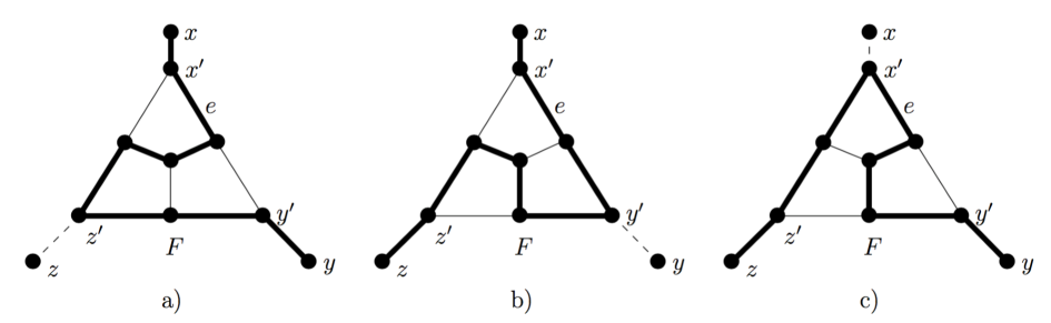
Figure 12: The gadget $F$; the edges of Hamiltonian cycles are shown by the bold lines.

Suppose that $G$ has a Hamiltonian cycle $C$. Then $C$ contains two edges incident to $v$. We construct the Hamiltonian cycle in $G^{\prime}{}$ by replacing these two edges by paths shown in Fig. 12. If $C$ contains $\{x,v\}$ and $\{v,y\}$, then they are replaced by the path shown in Fig. 12 a), if $C$ contains $\{x,v\}$ and $\{v,z\}$, then they are replaced by the path shown in Fig. 12 b) and if $C$ contains $\{y,v\}$ and $\{v,z\}$, then we use the path shown in Fig. 12 c). It is easy to see that we obtain a Hamiltonian cycle that contains $e$. If $G^{\prime}{}$ has a Hamiltonian cycle, then it is straightforward to see that $G$ is Hamiltonian as well. ∎

Now we are ready to prove Theorem 1.3.

of Theorem 1.3.

We construct an AND-cross-composition of Hamiltonicity with a Given Edge. By Lemma 6.3, the problem is NP-complete. We assume that two instances $(G,e)$ and $(G^{\prime},e^{\prime}{})$ of Hamiltonicity with a Given Edge are equivalent if $|V(G)|=|V(G^{\prime})|$. Let $(G_{i},e_{i})$ for $i\in\{1,\ldots,t\}$ be equivalent instances of Hamiltonicity with a Given Edge, $|V(G_{i})|=n$. We construct the graph $G$ as follows (see Fig. 13).

• Construct disjoint copies of $G_{1},\ldots,G_{t}$.

• For each $i\in\{1,\ldots,t\}$, subdivide $e_{i}$ twice and denote the obtained vertices by $u_{i},v_{i}$.

• For $i\in\{1,\ldots,t\}$, construct an edge $\{v_{i},u_{i+1}\}$ assuming that $u_{n+1}=u_{1}$.

It is straightforward to see that $G$ is a cubic planar graph.

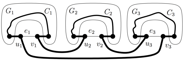
Figure 13: The construction of $G$ for $t=3$; the edges of a Hamiltonian cycle in $G$ are shown by the bold lines.

We claim that $G$ is $n+2$-cyclable if and only if $(G_{i},e_{i})$ is a yes-instance of Hamiltonicity with a Given Edge for every $i\in\{1,\ldots,t\}$. If every $G_{i}$ has a Hamiltonian cycle $C_{i}$ that contains $e_{i}$, then $G$ is Hamiltonian as well; the Hamiltonian cycle in $G$ is constructed from $C_{1},\ldots,C_{t}$ as it is shown in Fig. 13. Since $G$ is Hamiltonian, $G$ is $n+2$-cyclable. Suppose now that $G$ is $n+2$-cyclable. Let $i\in\{1,\ldots,t\}$. Consider $X=V(G_{i})\cup\{u_{i},v_{i}\}$. Because $|X|=n+2$, $G$ has a cycle $C$ that goes trough all the vertices of $X$. It remains to observe that by the removal of the vertices of $V(G)\setminus V(G_{i})$ and by the addition of the edge $e_{i}$, we obtain from $C$ a Hamiltonian cycle in $G_{i}$ that contains $e_{i}$. ∎

7 Discussion

Notice that we have no proof (or evidence) that Cyclability is in NP. The definition of the problem classifies it directly in ${\sf\Pi}_{2}^{\rm P}$. This prompts us to conjecture the following:

Conjecture 7.1.

Cyclability is ${\sf\Pi}_{2}^{\rm P}$-complete.

Moreover, while we have proved that Cyclability is co-W[1]-hard, we have no evidence which level of the parameterized complexity hierarchy it belongs to (lower than the XP class). We find it an intriguing question whether there is some $i\geq 1$ for which Cyclability is ${\sf W}[i]$-complete (or ${\sf co}\mbox{-}{\sf W}[i]$-complete).

Clearly, a challenging question is whether the, double exponential, parametric dependance of our FPT-algorithm can be improved. We believe that this is not possible and we suspect that this issue might be related to Conjecture 7.1.

Another direction of research is whether Cyclability is in FPT on more general graph classes. Actually, all results that were used for our algorithm can be extended on graphs embeddable on surfaces of bounded genus – see [24, 10, 34, 35, 27] – and yield an FPT-algorithm on such graphs (with worst time bounds). We believe that this is still the case for graph classes excluding some fixed graph as a minor. However, in our opinion, such an extension even though possible would be too technically involved.

References

- [1] Adler, I., Dorn, F., Fomin, F.V., Sau, I., Thilikos, D.M.: Fast minor testing in planar graphs. In: Algorithms - ESA 2010, 18th Annual European Symposium (1). Lecture Notes in Computer Science, vol. 6346, pp. 97–109. Springer (2010)
- [2] Adler, I., Kolliopoulos, S.G., Krause, P.K., Lokshtanov, D., Saurabh, S., Thilikos, D.M.: Tight bounds for linkages in planar graphs. In: Automata, Languages and Programming - 38th International Colloquium, ICALP 2011. Lecture Notes in Computer Science, vol. 6755, pp. 110–121. Springer (2011)
- [3] Aldred, R.E., Bau, S., Holton, D.A., McKay, B.D.: Cycles through 23 vertices in 3-connected cubic planar graphs. Graphs and Combinatorics 15(4), 373–376 (1999)
- [4] Bodlaender, H.L.: A linear-time algorithm for finding tree-decompositions of small treewidth. SIAM J. Comput. 25(6), 1305–1317 (1996)
- [5] Bodlaender, H.L., Fomin, F.V., Lokshtanov, D., Penninkx, E., Saurabh, S., Thilikos, D.M.: (meta) kernelization. In: Proceedings of the 2009 50th Annual IEEE Symposium on Foundations of Computer Science. pp. 629–638. FOCS ’09, IEEE Computer Society, Washington, DC, USA (2009)
- [6] Bodlaender, H.L., Jansen, B.M.P., Kratsch, S.: Kernelization lower bounds by cross-composition. SIAM J. Discrete Math. 28(1), 277–305 (2014)
- [7] Courcelle, B.: The monadic second-order logic of graphs. I. Recognizable sets of finite graphs. Information and Computation 85(1), 12–75 (1990)
- [8] Courcelle, B., Engelfriet, J.: Graph Structure and Monadic Second-Order Logic - A Language-Theoretic Approach, Encyclopedia of mathematics and its applications, vol. 138. Cambridge University Press (2012)
- [9] Cygan, M., Fomin, F.V., Kowalik, L., Lokshtanov, D., Marx, D., Pilipczuk, M., Pilipczuk, M., Saurabh, S.: Parameterized Algorithms. Springer (2015).
- [10] Demaine, E.D., Hajiaghayi, M., Thilikos, D.M.: The bidimensional theory of bounded-genus graphs. SIAM J. Discrete Math. 20(2), 357–371 (2006)
- [11] Diestel, R.: Graph theory, Graduate Texts in Mathematics, vol. 173. Springer, Heidelberg, fourth edn. (2010)
- [12] Dirac, G.A.: In abstrakten Graphen vorhandene vollständige 4-Graphen und ihre Unterteilungen. Math. Nachr. 22, 61–85 (1960)
- [13] Downey, R.G., Fellows, M.R.: Parameterized complexity. Springer-Verlag, New York (1999)
- [14] Downey, R., Fellows, M.: Fixed-parameter tractability and completeness. III. Some structural aspects of the hierarchy. In: Complexity theory, pp. 191–225. Cambridge Univ. Press, Cambridge (1993)
- [15] Downey, R.G., Fellows, M.R.: Fixed-parameter tractability and completeness. In: 21st Manitoba Conference on Numerical Mathematics and Computing (Winnipeg, MB, 1991), vol. 87, pp. 161–178 (1992)
- [16] Downey, R.G., Fellows, M.R.: Fixed-parameter tractability and completeness. I. Basic results. SIAM J. Comput. 24(4), 873–921 (1995)
- [17] Downey, R.G., Fellows, M.R.: Fixed-parameter tractability and completeness II: On completeness for . Theoretical Computer Science 141(1-2), 109–131 (1995)
- [18] Downey, R.G., Fellows, M.R.: Fundamentals of Parameterized Complexity. Texts in Computer Science, Springer (2013)
- [19] Erdős, P.: Remarks on a paper of Pósa. Magyar Tud. Akad. Mat. Kutató Int. Közl. 7, 227–229 (1962)
- [20] Flandrin, E., Li, H., Marczyk, A., Woźniak, M.: A generalization of dirac’s theorem on cycles through vertices in -connected graphs. Discrete mathematics 307(7), 878–884 (2007)
- [21] Flum, J., Grohe, M.: Parameterized Complexity Theory. Springer (2006)
- [22] Fomin, F.V., Golovach, P.A., Thilikos, D.M.: Contraction obstructions for treewidth. J. Comb. Theory, Ser. B 101(5), 302–314 (2011)
- [23] Garey, M.R., Johnson, D.S., Tarjan, R.E.: The planar Hamiltonian circuit problem is NP-complete. SIAM J. Comput. 5(4), 704–714 (1976)
- [24] Geelen, J.F., Richter, R.B., Salazar, G.: Embedding grids in surfaces. European J. Combin. 25(6), 785–792 (2004)
- [25] Grötschel, M.: Hypohamiltonian facets of the symmetric travelling salesman polytope. Zeitschrift für Angewandte Mathematik und Mechanik 58, 469–471 (1977)
- [26] Gu, Q.P., Tamaki, H.: Improved bounds on the planar branchwidth with respect to the largest grid minor size. In: Algorithms and Computation - 21st International Symposium, (ISAAC 2010). pp. 85–96 (2010)
- [27] Kawarabayashi, K.i., Wollan, P.: A shorter proof of the graph minor algorithm: The unique linkage theorem. In: Proceedings of the Forty-second ACM Symposium on Theory of Computing. pp. 687–694. STOC ’10, ACM, New York, NY, USA (2010)
- [28] Niedermeier, R.: Invitation to fixed-parameter algorithms. Habilitation thesis, (Sep 2002)
- [29] Perkovic, L., Reed, B.A.: An improved algorithm for finding tree decompositions of small width. Int. J. Found. Comput. Sci. 11(3), 365–371 (2000)
- [30] Plummer, M., Győri, E.: A nine vertex theorem for 3-connected claw-free graphs. Studia Scientiarum Mathematicarum Hungarica 38(1), 233–244 (2001)
- [31] Robertson, N., Seymour, P.: Graph minors. xxii. irrelevant vertices in linkage problems. Journal of Combinatorial Theory, Series B 102(2), 530 – 563 (2012)
- [32] Robertson, N., Seymour, P.D.: Graph Minors. X. Obstructions to Tree-decomposition. J. Combin. Theory Series B 52(2), 153–190 (1991)
- [33] Robertson, N., Seymour, P.D.: Graph minors .xiii. the disjoint paths problem. J. Comb. Theory, Ser. B 63(1), 65–110 (1995)
- [34] Robertson, N., Seymour, P.D.: Graph Minors. XIII. The disjoint paths problem. J. Combin. Theory Ser. B 63(1), 65–110 (1995)
- [35] Robertson, N., Seymour, P.D.: Graph minors. XXI. Graphs with unique linkages. J. Combin. Theory Ser. B 99(3), 583–616 (2009)
- [36] Watkins, M., Mesner, D.: Cycles and connectivity in graphs. Canad. J. Math 19, 1319–1328 (1967)