Infinite volume extrapolation in the one-dimensional bond diluted Levy spin-glass model near its lower critical dimension

Abstract

We revisited, by means of numerical simulations, the one dimensional bond diluted Levy Ising spin glasses outside the limit of validity of mean field theories. In these models the probability that two spins at distance $r$ interact (via a disordered interactions, $J_{ij}=\pm 1$) decays as $r^{-\rho}$. We have estimated, using finite size scaling techniques, the infinite volume correlation length and spin glass susceptibility for $\rho=5/3$ and $\rho=9/5$. We have obtained strong evidence for divergences of the previous observables at a non zero critical temperature. We discuss the behavior of the critical exponents, especially when approaching the value $\rho=2$, corresponding to a critical threshold beyond which the model has no phase transition. Finally, we numerically study the model right at the threshold value $\rho=2$.

I Introduction and model definition

The study of spin glasses on finite dimensional lattices is a notoriously difficult problem, because of very strong finite size effects. Recently, there has been a renewed interested in long range models, since these allow to interpolate between mean-field critical behavior and finite dimensional one. In particular, the diluted version of these long range models is very efficient and allows us to simulate very large sizes, thus reducing the finite size effects.

In the present work we show that for these diluted models with long range interactions it is actually possible to extract the asymptotic scaling functions from the numerical data. These functions allow us to estimate the values of the observables in the thermodynamic limit, and consequently to estimate the critical behavior in an alternative way than the one already used in Ref. Leuzzi08, . In addition, we want to extract the elusive correction-to-scaling exponent to compare with previous numerical computations. Leuzzi08

Another interesting issue is the understanding of the behavior of the Ising spin glass model near its lower critical dimension focusing on the breakdown of scaling laws (e.g. via logarithmic corrections). In the Edward-Anderson model, the lower critical dimension was estimated in Ref. Franz, as $D_{\mathrm{L}}=2.5$ and recently it has been studied experimentally in (thin) spin glass films. Orbach We can also study this issue in the long range model by tuning the power law decay exponent of the couplings.

We study the one dimensional Ising spin glass ($\sigma_{i}=\pm 1$) with Hamiltonian Leuzzi08 ; Leuzzi09

$${\cal H}=-\sum_{i<j}J_{ij}\sigma_{i}\sigma_{j}\,\,.$$ (1)

The quenched random couplings $J_{ij}$ are independent and identically distributed random variables taking a non zero value with a probability decaying with the distance between spins $\sigma_{i}$ and $\sigma_{j}$, $r_{ij}\equiv\min(|i-j|,L-|i-j|)$, as

$$\mathbf{P}[J_{ij}\neq 0]\propto r_{ij}^{-\rho}\quad\text{for}\;\;r_{ij}\gg 1\;.$$ (2)

Non-zero couplings take value $\pm 1$ with equal probability. We use periodic boundary conditions and a $z=6$ average coordination number.

We will briefly review the most important characteristic of this model. The most important point is that the $\rho$ parameter determines the universality class of the model. In Table 1 the different critical behaviors as a function of the value of $\rho$ are reported.

$\rho$	$D(\rho)$	transition type
$\leq 1$	$\infty$	Bethe lattice like
$(1,4/3]$	$[6,\infty)$	$2^{\rm nd}$ order, MF
$(4/3,2]$	$[2.5,6)$	$2^{\rm nd}$ order, non-MF
$2$	$2.5$	Kosterlitz-Thouless or $T=0$-like
$>2$	$<2.5$	none

Table 1: From infinite range to short range behavior of the SG model defined in Eqs.(1,2).

For $\rho>1$ the critical behavior turns out to be equal to the one of the fully connected version of the model, FT_LR where bonds are Gaussian distributed with zero mean and a variance depending on the distance as ${\overline{J_{ij}^{2}}}\propto r_{ij}^{-\rho}$. By changing $\rho$, the model displays different behaviors: Leuzzi08 for $\rho\leq\rho_{\mathrm{U}}\equiv 4/3$, the mean-field (MF) approximation is exact, while for $\rho>\rho_{\mathrm{U}}$, infrared divergences arise and the MF approximation breaks down. The value $\rho_{\rm U}=4/3$ marks the equivalent of the upper critical dimension of short-range spin-glasses in absence of an external magnetic field ($D_{\rm U}=6$). At $\rho>\rho_{\rm L}=2$ no finite temperature transition occurs, even for zero magnetic field, $h=0$. Campanino87 A relationship between $\rho$ and the dimension $D$ of short-range models can be expressed as $\rho=1+2/D$ which is exact at $D_{\rm U}=6$ ($\rho_{\rm U}=4/3$) and approximated as $D<D_{\rm U}$. Indeed, according to this analogy, the lower critical dimension $D_{\rm L}\simeq 2.5$(see Refs. Franz, and Boettcher05, ) would correspond to $\rho\simeq 1.8$, rather than to $\rho=\rho_{\rm L}=2$. An improved equation relating short-range dimensionality $D$ and power-law long-range exponent $\rho$ includes the value of the critical exponent of the space correlation function for the short-range model, $\eta(D)$, and reads: KYultimo

$$\rho(D)=1+\frac{2-\eta(D)}{D}\,.$$ (3)

In systems whose lower critical dimension is not fractional and $\eta(D_{\rm L})$ can be explicitely estimated the above relationship guarantees, at least, that $\rho(D_{\rm L})=\rho_{\rm L}$, though some discrepancies have been observed, as well, in between $\rho_{\rm U}$ and $\rho_{\rm L}$, see, e.g., Refs. [Banos12, ; Ibanez13, ; Leuzzi13, ; Angelini14, ].

A large number of studies concentrated on the parameter region around the threshold between mean-field-like behavior and non-mean-field one ($\rho_{\mathrm{MF}}=4/3$). The present work focuses, instead, on large values of $\rho$ ($\rho=5/3,9/5,2$), whose critical behavior is similar to the behavior of short-range interacting models in low dimension, close to the lower critical one. As expected in general for low dimensional systems, these models show more severe finite size effects than previously studied cases. The aim of the present analysis is to show that a faithful extrapolation of the critical behavior in the thermodynamic limit can be achieved also in these harder cases, by means of improved finite size scaling techniques. These techniques are based on those developed in Ref. [Caracciolo95, ] and involve the estimate of the leading correction-to-scaling exponent. In this paper we will provide a comprehensive study of these scaling correction tackling with the confluent (analytical) corrections and the non-confluents ones.

Finally, a further motivation for this numerical study is the comparison with an analytical estimate of the divergence of the correlation length in the $\rho=2$ model obtained by Moore,Moore10 (for $\rho=2$ the model is at its lower critical dimension). In addition, we are interested to research possible logarithmic corrections to the scaling laws just at the lower critical dimension.

II Observables and the Finite Size Scaling Method

The onset of spin glass long range order can be studied using the four-point correlation function

$$C(x)=\sum_{i=1}^{L}{\overline{\langle\sigma_{i}\sigma_{i+x}\rangle^{2}}}$$ (4)

where indices should be intended modulo $L$ and we have denoted the average over quenched disorder by $\overline{(\cdot\cdot\cdot)}$ and the thermal average by $\langle(\cdot\cdot\cdot)\rangle$. In terms of Fourier transform $\tilde{C}(k)$ one can express both the SG susceptibility

$$\chi_{\rm sg}\equiv\tilde{C}(0)$$ (5)

and the so-called second-moment correlation lengthCaracciolo95

$$\xi_{2}\equiv\frac{L}{2\pi}\left[\frac{\tilde{C}(0)}{\tilde{C}(2\pi/L)}-1\right]^{\frac{1}{\rho-1}}\;$$ (6)

Notice that, for the simulated lattice sizes $\sin(\pi/L)\simeq\pi/L$.

We will describe in the next paragraphs the Finite Size Scaling (FSS) method that we have used to analyze the data. Caracciolo95 Consider a singular observable $O$ diverging at the critical temperature $T_{c}$ as $|T-T_{c}|^{-y_{O}}$. Discarding corrections to scaling, we can write

$$\frac{O(T,L)}{O(T,\infty)}=f_{O}\left(\frac{\xi_{2}(T,\infty)}{L}\right)\,,$$ (7)

being $f_{O}(x)$ an universal function, decaying at large $x$ as $f_{O}(x)\sim x^{-y_{O}/\nu}$. For the observables of our interest, i.e., spin glass susceptibility and correlation length, we have $y_{\chi}=\gamma$ and $y_{\xi_{2}}=\nu$ and, therefore,

$$f_{\chi}(x) \sim x^{-\gamma/\nu}=x^{1-\rho}$$ (8)

$$f_{\xi_{2}}(x) \sim 1/x\qquad\qquad\qquad\text{for }x\to\infty$$

where we have used the fact the $\eta$ exponent does not renormalize in long-range systems and takes the value $\eta=3-\rho$.

From Eq. (7), we can write, as well,

$$\frac{O(T,2L)}{O(T,L)}=F_{O}\left(\frac{\xi_{2}(T,L)}{L}\right)\,,$$ (9)

where $F_{O}$ is another universal function.

To extrapolate our measures to infinite volume, we have followed the procedure described in Refs. Caracciolo95, and Palassini99, . We perform Monte Carlo simulations on different pairs $(T,L)$ computing generic observables, $O(T,L)$, among which, in particular, the correlation length, $\xi_{2}(L,T)$. This allows us to plot $O(T,2L)/O(T,L)$ against $\xi_{2}(T,L)/L$: if all the points lie on the same curve, Eq. (9) holds and the scaling corrections are negligible. We can, thus, compute the scaling functions $F_{O}$ and $F_{\xi_{2}}$. From these we can iteratively extrapolate the infinite volume pair $(\xi_{2},O)$. In our simulations we approach the $L\to\infty$ limit along the sequence $L\to 2L\to 2^{2}L\to\cdot\cdot\cdot\to\infty$. In order to do such an extrapolation we need a smooth interpolating function for $F_{O}(z)$.

For short range models, previous studies Caracciolo95 ; Palassini99 used interpolating functions of the kind

$$F_{O}(x)=1+\sum_{k=1}^{n}a_{k}^{O}\exp(-k/x)\,,$$ (10)

where the coefficients $a_{k}^{O}$ depend on the observable $O$ and, typically, $n\simeq 4$. This functional form was based on the theory of the two dimensional $O(3)$ model Caracciolo95 and worked satisfactorily in the three dimensional Ising spin glass. Palassini99

In the present case Eq. (10) does not interpolate well the numerical data and we need to resort to a different functional form. We have, thus, introduced the following parameterization of the scaling functions $F_{\xi_{2}}$ and $F_{\chi}$:

$$F_{O}(z)=1+\frac{a_{1}z}{a_{2}+z}+\frac{a_{3}z}{a_{4}+z}\,.$$ (11)

where the $a$’s coefficients depend on the choice of the observable $O$ and for $O=\xi_{2}$ they must satisfy the constraint $a_{1}+a_{3}=1$. This parameterization works really well for all values of $\rho$ and for both the measured correlation length and spin glass susceptibility. In the $\rho=2.0$ case we have used, as well, 7th and 8th degree cubic spline polynomial fitsNUMREC to compare with the new interpolation proposed.

III Numerical Simulations

We have simulated the model using the Metropolis algorithm and multi-spin coding (we have simulated 64 systems in parallel). In addition, to thermalize samples in the low temperature region we have used the parallel tempering method. PT In order to check thermalization we have looked at the temporal evolution of each observable measured on a logarithmic time scale. In Table 2 we report all the parameters used in our simulations. As a control, we have also simulated small lattices.

	$N_{s}$
$B$	$\rho=5/3$	$\rho=9/5$	$\rho=2$
6	154624	119808	64000
7	113536		320000
8	39936	178688	6656
9	21632	33792	45056
10	29824	154368	12544
11	54912	92160	24064
12	38784	38912
13	16512
$[T_{m},T_{M}]$	$[1.4,2.8]$	$[1.1,2.2]$	$[0.5,2.3]$
$\Delta T$	0.05	0.05	0.05

Table 2: Parameters of the numerical simulations. $B\equiv\log_{2}L$, $N_{s}$ is the number of samples, and $T_{m}$, $T_{M}$ and $\Delta T$ are the lowest temperature, the highest one and the temperature step in the parallel tempering method.

IV Numerical Results for the Critical Behavior

IV.1 Critical behavior for $\rho=5/3$ ($3<D<4$)

In Fig. 1 we test the Finite Size Scaling Ansatz in the form of Eq. (9). We can still see weak scaling corrections for the smallest plotted value of the lattice size ($2^{9}$), but all data for larger sizes lie on the same curves both for the susceptibility (top panel of Fig. 1) and the correlation length (bottom panel of Fig. 1). The next step is to interpolate the data with the scaling function defined in Eq. (11). The fit is good with a $\chi^{2}/\mathrm{d.o.f.}$ equal to $5.1/26$ and $3.2/25$ for the $\xi_{2}$ and $\chi$, respectively (discarding the $x$-error bars). Statistical errors on the extrapolated observables ($\xi(T)$ and $\chi(T)$) are estimated using the same Monte Carlo technique introduced in Ref. [Caracciolo95, ].

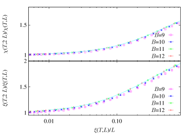
Figure 1: (color online) Rescaled data for $\rho=5/3$ according to Eq. (9) and interpolating FSS functions $F_{\chi}$ (top) and $F_{\xi_{2}}$ (bottom) for sizes $L=2^{B}$. Error bars are smaller than symbol sizes. The two continuous lines are the fits performed with Eq. (11). In the figures of this paper we will use $\xi$ as $\xi_{2}$.

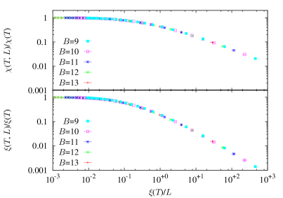
Figure 2: (color online) Rescaled data for $\rho=5/3$ according to Eq. (7).

Once we have the extrapolated values of $\xi_{2}$ and $\chi$, as a consistency test, we check if Eq. (7) holds. We present this test in Fig. 2. We can see that all the points are lying on the same universal curves corresponding to $f_{\chi}$ (top) and $f_{\xi_{2}}$ (bottom). For large $x$ a simple fitting procedure returns $f_{\xi_{2}}(x)\sim x^{-0.91(5)}$ and $f_{\chi}(x)\sim x^{-0.59(4)}$, not far from the behavior predicted Eq. (8), but nevertheless underestimating the exponent values. However, data in Fig. 2 clearly show a downward bending, even for the largest $\xi(T)/L$, thus suggesting that finite size effects still prevent a proper asymptotic estimate for the exponents (so, we need to take into account scaling corrections). An improved test can be obtained by plotting the quantity

$$C(O,L,T)\equiv x^{y_{O}/\nu}f_{O}(x)$$ (12)

versus $1/x\equiv L/\xi(T)$, that is expected to extrapolate to a finite value on the $y$ axis (as $L/\xi(T)\to 0$ or equivalently $\xi(T)\to\infty$). The results of this test clearly confirm this behavior, as shown in Fig. 3.

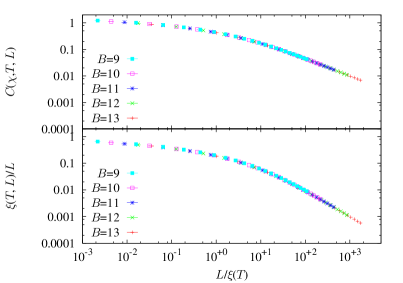
Figure 3: (color online) Test on the scaling functions $f_{\chi}$ and $f_{\xi}$ for $\rho=5/3$. We plot $C(O,T,L)\equiv x^{y_{O}/\nu}f_{O}(x)$ versus $1/x\equiv L/\xi(T)$ ($O=\xi,\chi$). Notice that $C(\xi,T,L)=\xi(T,L)/L$.

Using the interpolating functions for $F_{\chi}$ and $F_{\xi_{2}}$ (see Fig. 1) we can extrapolate susceptibility and correlation length to the thermodynamic limit. In Fig. 4 we show the resulting infinite volume susceptibility, which is well fitted by the usual power law, including scaling corrections,

$$\chi=A\xi_{2}^{2-\eta}\left(1+B\xi_{2}^{-\Delta}\right)+C.$$ (13)

Notice that the constant $C$ in the fit takes into account the background in the susceptibility induced by the analytic part of the free energy.

Fitting in the range $\xi_{2}>10$ we obtain: $\eta=1.353(15)$ and $\Delta=0.4(1)$ ($\chi^{2}/\mathrm{d.o.f.}=4.5/12$). Eventually, we can exploit the knowledge of the exact value $\eta=3-\rho=4/3$ and find a better estimate for the correction-to-scaling exponent $\Delta=0.28(2)$ ($\chi^{2}/\mathrm{d.o.f.}=5.4/13$).

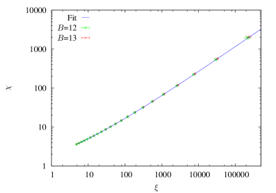
Figure 4: (color online) Extrapolated thermodynamical susceptibility $\chi$ versus $\xi_{2}$ for $\rho=5/3$. The two data sets correspond to extrapolations obtained by using up to $B=13$ data (red points) and up to $B=12$ data (green points).

The final step of the analysis is to compute the critical temperature $T_{c}$, the correlation length exponent $\nu$, and the scaling correction exponent $\theta$, according to the following equation

$$\xi_{2}(T,\infty)=A(T-T_{c})^{-\nu}\left(1+B(T-T_{c})^{\theta}\right)\,.$$ (14)

By fitting the data in the range $T\leq 2.3$ we obtain $T_{c}=1.35(1)$, $\nu=5.0(3)$ and $\theta=1.9(1)$ with a $\chi^{2}/\mathrm{d.o.f.}=5.4/13$, cf. Fig. 5.

If we associate $\Delta$ and $\theta$ to non-confluent scaling corrections, one should have $\theta=\nu\Delta$. Taking the estimates of $\nu$ and $\theta$ from the $\xi_{2}$-fit, we obtain $\theta/\nu=0.38(3)$, which compares well with the values obtained for $\Delta$ from the $\chi$ versus $\xi_{2}$ fit.

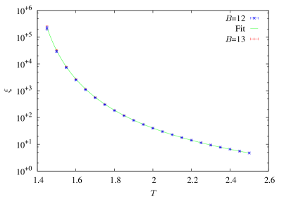
Figure 5: (color online) $\rho=5/3$. Extrapolated thermodynamical correlation length $\xi_{2}$ versus temperature, together with the best fit. The two data sets correspond to extrapolations obtained by using up to $B=13$ data (red points) and up to $B=12$ data (green points).

As an additional test of the extrapolation procedure, we show in Figs. 4 and 5 the infinite volume results obtained using data from simulations of system sizes up to $B=12$ (green points) and up to $B=13$ (red points), that coincide very well within the errors.

Finally, we can compare the above results with previous estimates Leuzzi08 obtained using the quotient method: quotient $T_{c}=1.36(1)$, $\nu=5.3(8)$ and $\omega=0.8(1)$. While $T_{c}$ and $\nu$ agree well, the correction-to-scaling exponent $\omega$ is different from the $\Delta$ exponent measured here. A similar disagreement on the value of the correction to scaling exponent in long range models has been recently observed in Ref. Angelini14, .

IV.2 Critical behavior for $\rho=9/5$ ($D_{\rm L}<D<3$)

We will be following the same procedure to extract the critical exponents as described in the previous subsection. In Fig. 6 we test the Finite Size Scaling Ansatz in the form of Eq. (9). Also for this value of $\rho$ all the data from different lattice sizes, but the smallest one, lie on the same universal curve both for the susceptibility (top panel) and the correlation length (bottom panel). The next step is to parameterize the two universal functions by means of a fit. The fits proposed in references [Caracciolo95, ,Palassini99, ] fail again for this value of $\rho$. We have rather used that of Eq. (11) for the interpolation, displaying a $\chi^{2}/\mathrm{d.o.f.}=15.7/17$ for the susceptibility and $\chi^{2}/\mathrm{d.o.f.}=1.1/18$ for the correlation length.

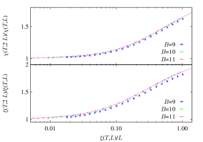
Figure 6: (color online) FSS functions $F_{\xi_{2}}$ (below) and $F_{\chi}$ (above)for $\rho=9/5$. We plot data for lattice sizes $2^{B}$ with $B=9,10,11$ and $12$. The error bars are less than the size of the symbols. The two continuous lines are the fits using Eq. (11).

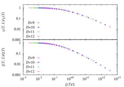
Figure 7: (color online) FSS functions $f_{\xi_{2}}$ (below) and $f_{\chi}$ for $\rho=9/5$. (above). The error bars are less than the size of the symbol

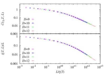
Figure 8: (color online) Test on the scaling functions $f_{\chi}$ and $f_{\xi}$ for $\rho=9/5$. We plot $C(O,T,L)\equiv x^{y_{O}/\nu}f_{O}(x)$ versus $1/x$ ($O=\xi,\chi$). Notice that $C(\xi,T,L)=\xi(T,L)/L$.

We show in Fig. 7 the scaling behavior of $\xi_{2}$ and $\chi$. By fitting the tails, taking into account the statistical error in both variables, we find $f_{\xi_{2}}(x)\sim x^{-0.89(5)}$ and $f_{\chi}(x)\sim x^{-0.70(3)}$. These results are to be compared with $f_{\xi_{2}}(x)\sim x^{-1}$ and $f_{\chi}(x)\sim x^{-0.8}$. Once again the scaling exponents turn out to be underestimated. To gain a deeper insight on this issue, we, therefore, plot $C(O,T,L)$ versus $L/\xi(T)$ in Fig. 8 obtaining finite extrapolated values as $L/\xi(T)\to 0$.

Using the $F_{O}$ and $F_{\xi_{2}}$ functions (see Fig. 6) we can extrapolate the finite volume correlation length and susceptibility to the thermodynamic limit. In Fig. 9 we present our results for the infinite volume susceptibility. We have fitted the data shown in Fig. 9 to Eq. (13), and we have obtained (discarding data with $\xi_{2}<15$) $\eta=1.221(15)$ and $\Delta=0.36(7)$ ($\chi^{2}/\mathrm{d.o.f.}=4.5/14$), while, assuming $\eta=3-\rho=1.2$, we obtain $\Delta=0.30(1)$ ($\chi^{2}/\mathrm{d.o.f.}=5.7/15$).

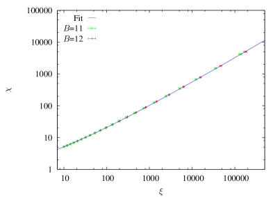
Figure 9: (color online) Extrapolated $\chi$ vs. $\xi_{2}$ for $\rho=9/5$. Notice the two sets of points: one corresponds to the extrapolation of the $B=12$-data (red) and the other one to the extrapolation of the $B=11$-data (green).

The final step is the analysis of the correlation length. By fitting the data to Eq. (14) (see Fig. 10) we obtain $T_{c}=0.961(8)$, $\nu=5.8(1)$ and $\theta=2.67(6)$ ($\chi^{2}/\mathrm{d.o.f.}=16.9/18$ with $T\leq 2.3$). Notice that $\theta/\nu=0.46(1)$, roughly compatible with the two estimates of $\Delta$.

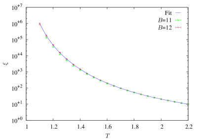
Figure 10: (color online) $\rho=9/5$. Extrapolated $\xi_{2}$ vs. $T$. We have plotted our best fit using Eq. (14) (see the text). Notice the two sets of points: one corresponds to the extrapolation of the $B=12$-data (red) and the other one to the extrapolation of the $B=11$-data (blue). The best fits is marked using a continuous green line.

As an additional test of the extrapolation procedure, we show in Figs. 9 and 10 the infinite volume data from system sizes up to $B=11$ and up to $B=12$: for this value of $\rho$ data turn out to be statistically compatible.

Finally, we can compare these results with the results obtained using the behavior of the non-zero Fourier momenta of the spin glass correlation function: Leuzzi11 $T_{c}=1.060(7)$.

IV.3 Critical behavior at the critical threshold exponent $\rho_{\rm L}=2$

As a last point we study numerically the model right at the value of $\rho$ corresponding to the lower critical dimension. In Fig. 11 we again test the Finite Size Scaling Ansatz in the form of Eq. (9). We can also see that, except for the $L=2^{6}$ system, which suffers stronger scaling corrections, all the data for larger lattice sizes lie on the same universal curve both for the susceptibility (top panel) and the correlation length (bottom panel). The next step has been to parameterize the two universal functions by means of numerical interpolation. The fits proposed in references [Caracciolo95, ,Palassini99, ] do not work for $\rho=2$. We have found, though, that a simple seventh- or eight-degree cubic spline polynomial fit works well for both observables. In addition, also fits following Eq. (11) work quite well (for $F_{\xi}$, $\chi^{2}/\mathrm{d.o.f.}=23.1/34$, and for $F_{\chi}$, $\chi^{2}/\mathrm{d.o.f.}=16.4/33$, again discarding the $x$-error bars). We present, in the following, the outcome of extrapolations according to Eq. (11).

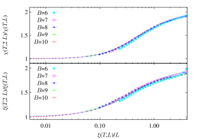
Figure 11: (color online) $\rho=2$. FSS functions $F_{\xi}$ (below) and $F_{\chi}$ (above). We plot data for $L=2^{6,7,8,9,10,11}$. We mark with the continuous line the fit to Eq.  (11).

Once again, we check if Eq. (7) holds. We present this test in Fig. 12. We can see that all the points, even those at $L=2^{6}$, are lying on the same universal curves (top panel for the susceptibility and bottom panel for the correlation length). By fitting the tails we obtain $f_{\xi_{2}}(x)\propto x^{-0.86(15)}$ and $f_{\xi_{2}}(x)\propto x^{-0.87(6)}$ (taking into account the error bars in both axes). One should expect that both scaling functions behave as $x^{-1}$, assuming that the relation $\eta=3-\rho$ is valid down to $\rho=2$. We, thus, repeated the analysis in term of $C(O,T,L)$, cf. Eq. (12), and the results are plotted in Fig. 13: one can see the expected behavior for small values of $L/\xi(T)$ (i.e. reaching a constant value).

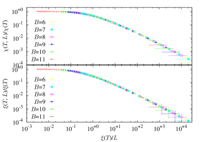
Figure 12: (color online) FSS functions $f_{\xi}$ (below) and $f_{\chi}$ (above) for $\rho=2$. We plot data for sizes $L=2^{6,7,8,9,10,11}$.

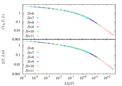
Figure 13: (color online) Test on the scaling functions $f_{\chi}$ and $f_{\xi}$ for $\rho=2$. We plot $C(O,T,L)\equiv x^{y_{O}/\nu}f_{O}(x)$ versus $1/x$ ($O=\xi,\chi$). Notice that $C(\xi,T,L)=\xi(T,L)/L$.

The extrapolated correlation length and susceptibility values to the thermodynamic limit are plotted in Figs. 14, 15. There we show the interpolations performed by means of Eq. (11) for data sizes up to $B=10$ and up to $B=11$ and also by means of the cubic spline fit. Our data for $\xi_{2}$ are well fitted by a law like

$$\xi(T,\infty)\propto\exp\left(\frac{a}{\sqrt{T}}\right)\,,$$ (15)

where $a=18.1(2)$ ($\chi^{2}/\mathrm{d.o.f.}=4.45/9$). The simulated numerical data are not compatible, though, with the law $\xi\propto\exp(-a\log T/T^{2})$ suggested by Moore, Moore10 (at least for $T\geq 0.5$), but it is worth reminding that the fully connected version studied by Moore and the diluted version we simulate may have a different critical behavior at $\rho=2$. Weigel

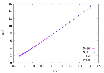
Figure 14: (color online) Extrapolated $\log\xi_{2}$ vs. $1/\sqrt{T}$ for $\rho=2$. We show points from the extrapolations of sizes up to $B=10$ and up to $B=11$, using Eq. (11). We also show the extrapolated points using the alternative fit by means of an eight degree cubic spline polynomial (on data up to $B=11$). The three extrapolations turn out to be in good agreement. For small values of the temperature the behavior (marked by “Fit” in the plot) is linear.

Finally, we analyze the relationship between susceptibility and correlation length. From a naive theoretical point of view, from the law $\chi\propto\xi^{2-\eta}$, we should expect a relation as $\chi\propto\xi$ in $\rho=2$, assuming $\eta=1$. This linear relation is possibly modified by logarithmic corrections. In Fig. 15 we plot $\log(\chi/\xi)$ versus $\log(\xi)$. One can see that finite size corrections to the leading behavior are there, though it is rather difficult to precisely determine their nature. Data are, indeed, consistent with logarithmic corrections, as well as power-law corrections with small exponents. The latter are estimated using data set of sizes up to $B=11$, either with an exponent $-0.08(4)$, using a large $\xi_{2}$ interpolation over points obtained by means of a cubic spline extrapolation, or with an exponent $-0.16(2)$, by means of Eq. (11). With the latter kind of behavior, one has $\chi\propto\xi^{1-0.16(2)}$, a bit different from the naive theoretical prediction. In any case, such small correction $\xi^{-0.16(2)}$ is very hard to be distinguished from a logarithmic correction.

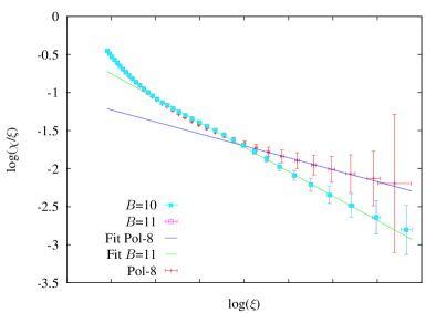
Figure 15: (color online) Extrapolated $\log(\chi/\xi)$ vs. $\log(\xi)$ for $\rho=2$, where logarithmic corrections can be appreciated. The large correlation length interpolation over points obtained by means of a cubic spline extrapolation (data set of sizes up to $B=11$) is consistent with a power law decay with exponent $-0.08(4)$. A even better power-law estimate is obtained using the extrapolation Eq. (11) on the same simulation data and yielding a decay exponent of or -0.16(2). Notice the consistency among all three extrapolations used.

V Discussion

In Fig. 16 we have plotted the behavior of $1/\nu$ as a function of $\rho$. Together with our numerical estimates, we have drawn the mean field prediction ($1/\nu=\rho-1$), which is valid for $\rho<4/3$ and the prediction from a first order renormalization group (RG) calculation, that should be valid very close to $\rho=4/3$. Since for $\rho=2$ we expect $1/\nu=0$, the decrease should be very fast and likely incompatible with the linear behavior $1/\nu\propto(2-\rho)$, predicted in Ref. Moore10, . Such a difference may be due to a possibly different critical behavior between the fully-connected and the diluted versions of the model. Weigel However another possibility is that one of the approximations made in Ref. Moore10, in order to solve the RG equations is too crude: actually the author of Ref. Moore10, warns the reader, just after Eq. (35), that the approximation made is not valid close to $T_{c}$ for $\rho<2$ (which is exactly the region we are studying).

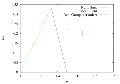
Figure 16: (color online) Behavior of $1/\nu$ as a function of $\rho$. The green straight line is the MF prediction ($1/\nu=\rho-1)$, the blue line is the results of the first order $\epsilon$-expansion and the points are from numerical simulations: the two rightmost points are from this work.

The behavior of the correlation length that we have found is consistent with the following renormalization flow of the temperature

$$\frac{dT}{dl}\propto T^{3/2}\,\,\,\mathrm{as}\,\,\,T\to 0\,,$$ (16)

whereas the phenomenological renormalization of Ref. Moore10, predicts a different leading behavior like

$$\frac{dT}{dl}\propto\frac{T^{3}}{\log T}\,\,\,\mathrm{as}\,\,\,T\to 0\,,$$ (17)

not compatible with our numerical data. This is another motivation to reconsider the approximation made in Ref. Moore10, .

VI Conclusions

We have numerically revisited the one dimensional bond diluted Levy Ising spin glass.Leuzzi08 ; Leuzzi09 In particular we have focused in the less explored region of power-law decaying interaction with large power-law exponents, not compatible with a mean-field critical behavior. Being $\rho=4/3$ the mean-field threshold, we have been analyzing data for the critical behavior of systems with $\rho=5/3,9/5$ and $2$. The latter being the exponent of the long-range model whose critical behavior is at zero temperature. Through a careful finite size scaling analysis we have been able to extrapolate, to infinite volume, refined susceptibility and correlation length scaling behaviors. These results allows us to test analytical predictions for the behavior at the lower critical dimension, corresponding to $\rho=2$, as the renormalization flow towards the zero temperature fixed point and the correlation length behavior in temperature. For the critical temperature flow our data are not compatible with the picture obtained in Ref. [Moore10, ] (see Ref. [Palassini99, ] for a similar discussion in the finite dimensional model). For the $\xi(T)$ behavior our data are compatible with Eq. (15) and not with the law proposed in Ref. [Moore10, ]. Quite generally, the methods used in this paper are very suitable for studying models near their lower critical dimension.

VII Acknowledgments

This work was partially supported by the Ministerio de Ciencia y Tecnología (Spain) through Grant No. FIS2013-42840-P, by the Junta de Extremadura (Spain) through Grant No. GRU10158 (partially founded by FEDER), by European Union through Grant No. PIRSES-GA-2011-295302, by European Research Council (ERC) through grant agreement No. 247328, by the Italian Ministry of Education, University and Research under the Basic Research Investigation Fund (FIRB/2008) through grants No. RBFR08M3P4 and RBFR086NN1, and under the PRIN2010 program, grant No. 2010HXAW77-008 and by the People Programme (Marie Curie Actions) of the European Union’s Seventh Framework Programme FP7/2007-2013/ under REA grant agreement n. 290038, NETADIS project.

References

- (1) L. Leuzzi, G. Parisi, F. Ricci-Tersenghi, and J. J. Ruiz-Lorenzo, Phys. Lett. Rev. 101, 107203 (2008).
- (2) G. Parisi, S. Franz and M. A. Virasoro, Journal de Physique I (France) 2, 1869-1880 (1992).
- (3) S. Guchhait and R. Orbach Phys. Rev. Lett. 112, 126401 (2013).
- (4) L. Leuzzi, G. Parisi, F. Ricci-Tersenghi, and J. J. Ruiz-Lorenzo, Phys. Rev. Lett. 103, 267201 (2009)
- (5) G. Kotliar, P.W. Anderson and D.L. Stein, Phys. Rev. B 27, 602 (1983). L. Leuzzi, J. Phys. A 32, 1417 (1999).
- (6) M. Campanino et al., Commun. Math. Phys. 108, 241 (1987).
- (7) S. Boettcher, Phys. Rev. Lett. 95, 197205 (2005).
- (8) H.G. Katzgraber, D. Larson and A.P. Young, Phys. Rev. Lett. 102, 177205 (2009).
- (9) R. A. Baños, L.A. Fernandez, V. Martin-Mayor, and A. P. Young, Phys. Rev. B 86, 134416 (2012).
- (10) M. Ibáñez Berganza and L. Leuzzi, Phys. Rev. B 88, 144104 (2013).
- (11) L. Leuzzi and G. Parisi, Phys. Rev. B 88, 224204 (2013).
- (12) M. C. Angelini, F. Ricci-Tersenghi, G. Parisi, Phys. Rev. E 89, 062120 (2014).
- (13) S. Caracciolo, R. G. Edwards, S. J. Ferreira, A. Pelissetto and A. D. Sokal, Phys. Rev. Lett. 74, 2969 (1995).
- (14) M. Moore, Phys. Rev. B 82, 014417 (2010).
- (15) M. Palassini and S. Caracciolo, Phys. Rev. Lett. 82, 5128 (1999).
- (16) W. H. Press, B. P. Flannery, S. A. Teukolsky and W. T. Vetterling, Numerical Recipes in C: The Art of Scientific Computing, Second Edition. (Cambridge University Press, Cambridge, 1992).
- (17) K. Hukushima and K. Nemoto, J. Phys. Soc. Japan 65, 1604 (1996).
- (18) H. G. Ballesteros, L. A. Fernandez, V. Martın-Mayor, and A. Munoz Sudupe, Phys. Lett. B 378, 207 (1996); 387, 125 (1996); Nucl. Phys. B 483, 707 (1997).
- (19) L. Leuzzi, G. Parisi, F. Ricci-Tersenghi, and J. J. Ruiz-Lorenzo, Philos. Mag. 91, 1917 (2011).
- (20) F. Beyer, M. Weigel, and M.A. Moore, Phys. Rev. B 86, 014431 (2012).