Pressure is not a state function for generic active fluids
Abstract
Pressure is the mechanical force per unit area that a confined system exerts on its container. In thermal equilibrium, it depends only on bulk properties (density, temperature, etc.) through an equation of state. Here we show that in a wide class of active systems the pressure depends on the precise interactions between the active particles and the confining walls. In general, therefore, active fluids have no equation of state; their mechanical pressures exhibit anomalous properties that defy the familiar thermodynamic reasoning that holds in equilibrium. The pressure remains a function of state, however, in some specific and well-studied active models that tacitly restrict the character of the particle-wall and/or particle-particle interactions.
For fluids in thermal equilibrium, the concept of pressure, , is familiar as the force per unit area exerted by the fluid on its containing vessel. This primary, mechanical definition of pressure seems to require knowledge of the interactions between the fluid’s constituent particles and its confining walls. But we learn from statistical mechanics that can also be expressed thermodynamically, as the derivative of a free energy with respect to volume. The pressure therefore obeys an equation of state, which only involves bulk properties of the fluid (temperature , number density , etc.). Hydrodynamics provides a third definition of , as the trace of the bulk thermodynamic stress tensor, whose microscopic definition in terms of momentum fluxes is again well known Allen . In thermal equilibrium, all these definitions of pressure coincide. The corresponding physical insight is that the fluid may be divided into blocks that are in mechanical equilibrium with each other and with any confining walls, so bulk and wall-based pressure definitions must agree.
Purely thermodynamic concepts, like temperature, are well known to be ill-defined in systems far from equilibrium Cugliandolo2011 . However, one could hope that mechanical properties, like pressure, are less problematic. Here we investigate this question for active fluids, in which energy dissipation at the microscopic level drives the motion of each particle to give strong non–equilibrium effects MarchettiRMP2013 . Assemblies of self-propelled particles (SPPs) have been proposed as simplified models for systems ranging from bacteria Bergbook ; CatesRRP2012 and active colloidal ‘surfers’ PalacciPRL2010 ; FilyPRL2012 ; ButtinoniPRL2013 , to shaken grains KudrolliPRL2008 ; NarayanSCI2007 and bird flocks BalleriniPNAS2008 . We define the mechanical pressure of an active fluid as the mean force per area exerted by its constituent particles on a confining wall. This was studied numerically for a number of active systems, showing some surprising effects for finite-size, strongly confined fluids MalloryPRE2014 ; FilySM2014 ; Fily2014 ; Niarxiv2014 ; Yang2014 ; TakatoriPRL2014 ; Takatoriarxiv2014 . Alternatively, when describing the dynamics of such active fluids at larger scales, some authors have introduced a bulk stress tensor and defined pressure as its trace MarchettiRMP2013 ; Yang2014 ; TakatoriPRL2014 ; Takatoriarxiv2014 , leading to recent experimental measurements GinotPRX2014 . Since we are far from equilibrium, an equivalence between these different definitions, as seen numerically in MalloryPRE2014 ; Yang2014 ; TakatoriPRL2014 , requires explanation.
In this article, we show analytically and numerically that the pressure exerted on a wall by generic active fluids directly depends on the microscopic interactions between the fluid and the wall. Unless these interactions, as well as the interactions between the fluid particles, obey strict and exceptional criteria, there is no equation of state relating the mechanical pressure to bulk properties of the fluid. Therefore, all connections to thermodynamics and to the bulk stress tensor are lost. Nevertheless, we provide analytical formulas to compute the wall-dependent pressure for some of the most studied classes of active systems. Exceptional models for which an equation of state is recovered include the strictly spherical SPPs considered in MalloryPRE2014 ; Yang2014 ; TakatoriPRL2014 . Below we find that such simplified models are structurally unstable: small orientation-dependent interactions (whether wall-particle or particle-particle) immediately destroy the equation of state. Such interactions are present in every experimental system we know of.
A clear distinction exists between the present work and that of Ref 20. The latter includes an explicit proof that pressure is, after all, well defined within a narrow class of models: spherical SPPs with torque-free wall interactions and torque-free pairwise interparticle forces. Because this class has been a major focus of theory and simulation studies, that finding is important, creating in those cases a direct link between pressure and correlation functions that can be exploited in future theoretical advances. However, in general terms it is even more important to know that an equation of state for the pressure is the exception, rather than the rule, in active matter systems. This we establish here.
To appreciate the remarkable consequences of the generic absence of an equation of state, consider the quasi-static compression of an active fluid by a piston. Since the mechanical pressure depends on the piston, compressing with a very soft wall—into which particles bump gently—or with a very hard one requires different forces and hence different amounts of work to reach the same final density. This is not the only way our thermodynamic intuition can fail for active systems. We will show both that pressure can be anisotropic, and that active particles admit flux-free steady-states in which the pressure is inhomogeneous. Finally, in the models we consider (which best describe, e.g., crawling bacteria Bergbook or colloidal surfers or rollers near a supporting surface PalacciSCI2014 ; BricardNAT2013 ) there are situations in which the confinement forces at the edges of a sample do not sum to zero. We show how this unbalanced force is compensated by momentum transfer to the support. The issue of whether an equation of state exists in so-called “wet” active matter MarchettiRMP2013 —in which full momentum conservation applies throughout the interior of the system—remains open.
Non–interacting particles
We consider a standard class of models for SPPs in which the independent Brownian motion of each particle (diffusivity ) is supplemented by self-propulsion at speed in direction ,
| (1) |
with a Gaussian white noise of unit variance. The reorientation of the direction of motion then occurs with a system-specific mechanism: active Brownian particles (ABPs) undergo rotational diffusion, while run-and-tumble particles (RTPs) randomly undergo complete reorientations (‘tumbles’) at a certain rate. These well-established models have been used FilyPRL2012 ; StenhammarPRL2013 ; RednerPRL2013 ; SchnitzerPRE1993 ; TailleurPRL2008 ; CatesRRP2012 ; CatesPNAS to describe respectively active colloids PalacciPRL2010 ; ButtinoniPRL2013 ; BricardNAT2013 ; PalacciSCI2014 , or bacterial motion Bergbook ; CatesPNAS and cell migration RTPcells . Such models neglect any coupling to a momentum conserving solvent, and are thus best suited to describe particles whose locomotion exploits the presence of a gel matrix or supporting surface as a momentum sink. This is true of many active systems, such as crawling cells SepulvedaPCB2013 , vibrated disks or grains DeseignePRL2010 ; NarayanSCI2007 ; KudrolliPRL2008 , and colloidal rollers BricardNAT2013 or sliders PalacciSCI2014 .
We address a system of SPPs with spatial coordinates in 2D; we assume periodic boundary conditions, and hence translational invariance, in the direction. The system is confined along by two walls at specified positions, which exert forces on particles at ; these forces have finite range and thus vanish in the bulk of the system. The propulsion direction of a particle is with along the direction. In the absence of interactions between the particles, the master equation for the probability of finding a particle at position at time pointing along the direction reads
| (2) |
Here and are the translational mobility and diffusivity; likewise and for rotations. The propulsive velocity is , and is the tumble rate. ABPs correspond to and RTPs to . Here we allow all intermediate combinations, to test the generality of our results. In addition to the external force , we include an external torque , which may, for example, describe the well–documented alignment of bacteria along walls ElgetiEPL2009 . Generically, just as in passive fluids, a wall–torque will arise whenever the particles are not spherical and its absence is thus strictly exceptional. Obviously, the asphericity of (say) water molecules does not violate the thermodynamical precepts of pressure; remarkably, we show below that, for active particles, it does so.
Since our setup is invariant along the direction, the mechanical pressure can be computed directly from the force exerted by the system on a wall (which we place at ), as
| (3) |
Here an origin is taken in the bulk, and is the steady-state density of particles at . As stated previously, for a passive equilibrium system () with the same geometry, the mechanical definition (3) of pressure is equivalent to the thermodynamic definition, as proved for completeness in the Supplementary Information (SI). Note that Eq. (3) still applies in the presence of other particles, such as solvent molecules, so long as those particles do not themselves exert any direct force on the wall (which is thus semi-permeable). Under such conditions is, by definition, an osmotic pressure; the results below will still apply to it, whenever Eq.(2) remains valid.
As described in the SI, the pressure can be computed analytically from Eq. (2) as:
| (4) |
This is a central result, and exact for all systems obeying Eq. (2). Clearly, in general depends on the wall-particle interactions, as does which is sensitive to both and . Thus the mechanical pressure obeying Eq. (4) is likewise sensitive to these details: it follows that no equation of state exists for active particle systems in the general case.
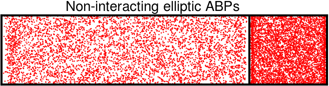
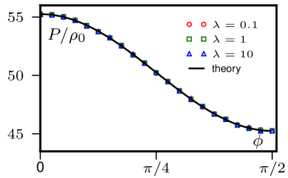
To illustrate this effect and show that (4) can indeed be used to compute the pressure, we study a model of ABPs with elliptical shape (see SI for details). We choose a harmonic confining potential, for , with otherwise, accompanied by a torque (again, for and zero otherwise). With , this is the torque felt by an elliptical particle of axial dimensions and unit area , subject to the linear force field distributed across its body. Assuming the steady-state distribution to relax to its bulk value outside the range of the wall potential, , the pressure in such an ABP fluid (for ) is given by
| (5) |
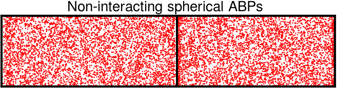
For the torque reduces the pressure by orienting the ABPs parallel to the wall. Equation (5) shows explicitly how walls with different spring constants experience different pressures, in sharp contrast with thermodynamics. We checked this prediction by direct numerical simulations of ABPs and found good agreement (see Fig. 1). We also found similar behavior numerically for (likewise elliptical) RTPs, confirming that the failure of thermodynamics is generic.
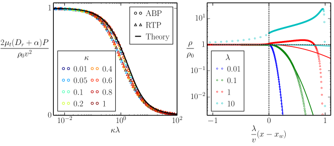
For passive particles in thermal equilibrium, and Eq. (4) reduces to the ideal gas law, , upon use of the Einstein relation (). Another case where an equation of state is recovered is for torque–free (e.g., spherical) particles, with . In that case Eq. (4) reduces to the same ideal gas law but with an effective temperature
| (6) |
This explains why previous numerical studies of torque–free, non–interacting active particle fluids gave consistent pressure measurements between impenetrable FilySM2014 ; Fily2014 or harmonically soft walls MalloryPRE2014 . Related expressions for the pressure of such fluids were found by computing the mean kinetic energy MalloryPRE2014 , or the stress tensor Yang2014 ; TakatoriPRL2014 ; Takatoriarxiv2014 , possibly encouraging a belief that all reasonable definitions of pressure in active systems are equivalent. However, Eq. (4) shows that these approaches cannot yield consistent results beyond the simplest, torque–free case.
The “effective gas law" of Eq. (6) for the torque–free case is itself remarkable. For ABPs or RTPs in an external potential , the effective temperature concept predicts a steady-state density that is accurate only for weak force fields TailleurEPL2009 ; ABPvsRTP . Yet Eq. (6) holds even with hard-core walls for which the opposite applies and the steady-state density profile is far from a Boltzmann distribution (see the simulation results of Fig. 1 and the analytical results for one–dimensional RTPs in SI). In fact the result stems directly from the exact computation of , which can be done at the level of the master equation and leads to Eq. (4), so that no broader validity of the concept is required, or implied.
Interacting active particles
Equation (4) gives the pressure of non–interacting active particles and we now address the extent to which our conclusions apply to interacting SPPs. Clearly, interactions will not restore the existence of an equation of state in the presence of wall torques and we thus focus on “torque-free” walls.
Interparticle alignment is probably the most studied interaction in active matter MarchettiRMP2013 . To measure its impact on pressure, we consider ABPs whose positions and orientations evolve according to (1) and
| (7) |
where is an aligning torque between the particles. As shown in SI, the pressure can be computed analytically to give
| (8) |
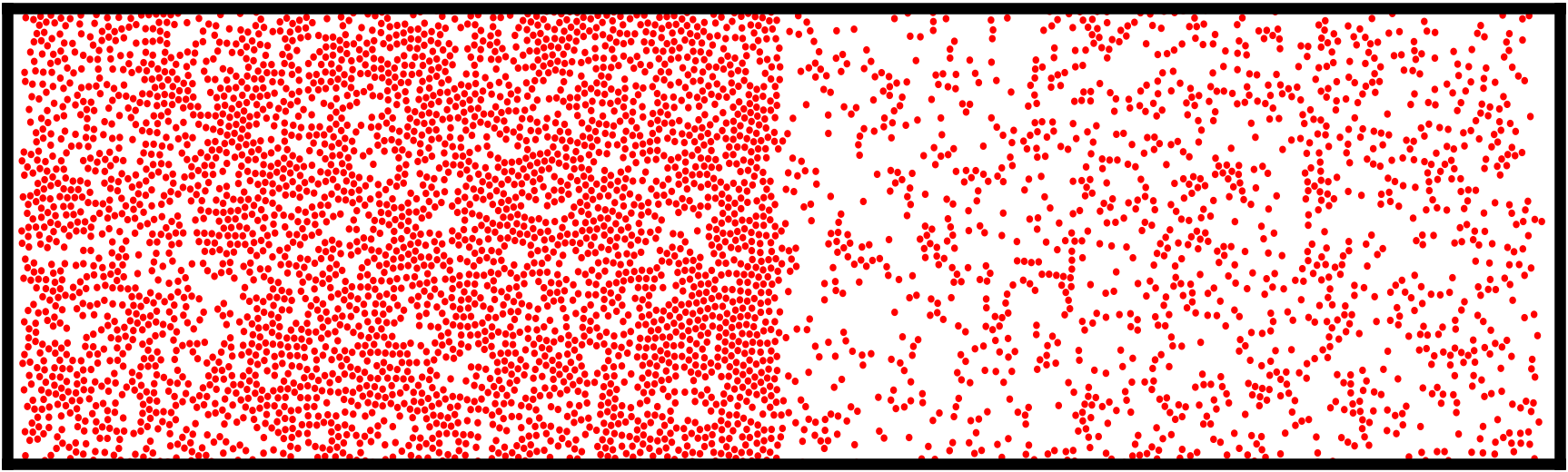
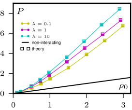
where the integral over is over the whole space. Since the distribution depends (for ) on the wall potential, so does the pressure. Therefore, even in the absence of wall torques, alignment interactions between particles destroy any equation of state. Figure 2 shows the result of ABP simulations with a particular choice of interparticle torque : The measured pressure indeed depends on the wall potential and agrees with equation (64).
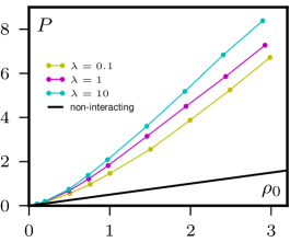
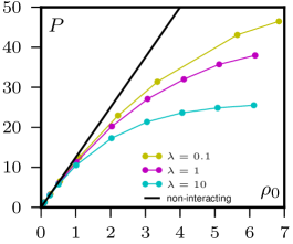
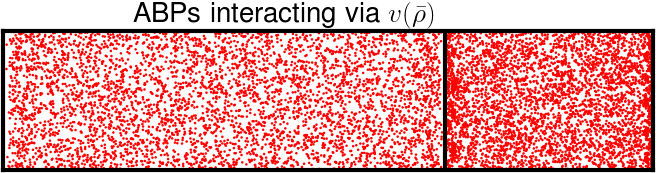
In active matter, more general interactions than pairwise torques often have to be considered. For example, in bacteria with “quorum sensing" (a form of chemical communication), particles at position can adapt their dynamics in response to changes in the local coarse–grained particle density LiuSCI2011 . Also shown in Fig. 2 are simulations for the case , reflecting a pairwise speed reduction (see SI for details). This is an example where even completely torque-free particles have no equation of state. Again, we show in SI how an explicit formula for the pressure can be computed from first principles.
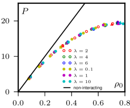
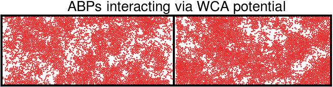
The case of torque–free ABPs with short range repulsive interactions RednerPRL2013 ; StenhammarPRL2013 ; LowenEPL2013 ; GompperEPL2013 was recently considered in Yang2014 ; TakatoriPRL2014 . The mechanical force exerted on a wall was found to coincide with a pressure computed from the bulk stress tensor, suggesting that in this case an equation of state does exist. To check this, we choose a Weeks–Chandler–Andersen (WCA) potential: if and otherwise, where is the inter-particle distance and the particle diameter. Using simulations we determined as a function of bulk density for various harmonic and linear wall potentials. As shown in Fig. 2, all our data collapses onto a wall-independent equation of state . An analytical expression for in this rather exceptional case is derived and studied in pressureABP in the context of phase equilibria.
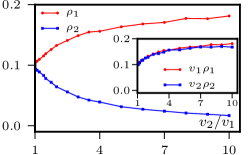
The cases explored above show that there is generically no equation of state in an active fluid, one exception being when wall-particle and particle-particle torques are both negligible. Given this outcome, a simple test for the presence or absence of an equation of state, in simulations or experiments, would be welcome. If the pressure is set by bulk properties of the fluid, when an asymmetrically interacting partition is used to separate the system in two parts, no force acts upon the partition and it does not move. Conversely, if the partition does move, there is no equation of state. To check this, we simulated a large box of homogeneous active fluid, introduced at its centre a mobile wall with asymmetric potentials on its two sides, and let the system reach steady state. In the cases shown above to have an equation of state, the wall remains at the center of the box so that the densities on its two sides stay equal. In the other cases, however, the partition moves to equalize the two wall–dependent pressures, resulting in a flux-free steady-state with unequal densities in the two chambers (Fig. 3).
Anomalous attributes of the pressure
A defining property of equilibrium fluids is that they cannot statically support an anisotropic stress. Put differently, the normal force per unit area on any part of the boundary is independent of its orientation. This applies even to oriented fluids (without positional order), such as nematic liquid crystals ChaikinLubensky , but breaks down for active nematics MarchettiRMP2013 .
We next show that it can also break down for active fluids with isotropic particle orientations, as long as the propulsion speed is anisotropic, i.e. . This could stem from an anisotropic mobility as might arise for cells crawling on a corrugated surface. We suppose so that oppositely oriented particles have the same speed; Eq. (2) then shows that the bulk steady state particle distribution remains isotropic. In addition, as shown in SI, the pressure acting on a wall whose normal is at angle to the axis remains independent of the wall interactions, but is -dependent; for RTPs () it obeys
| (9) |
To verify that the pressure is indeed anisotropic we performed numerical simulations for which show perfect agreement with Eq. (9) (see Fig. 4).
For passive fluids without external forces, mechanical equilibrium requires that the pressure is not only isotropic, but also uniform. This follows from the Navier–Stokes equation for momentum transport ChaikinLubensky , but also holds in (say) Brownian dynamics simulations which do not conserve momentum Allen .
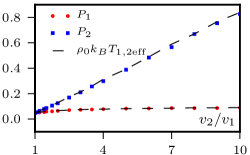
We now show that need not be uniform in active fluids, even when an equation of state exists. Consider non–interacting spherical ABPs in a closed container with different propulsion speeds in different regions, say for and for . This is a realizable laboratory experiment in active colloids whose propulsion is light-induced PalacciSCI2014 ; ButtinoniPRL2013 . From Eq. 2, the flux-free steady state has throughout SchnitzerPRE1993 ; TailleurPRL2008 ; CatesEPL2013 , so that the pressures are unequal. Though different, the pressures in the two compartments are well defined, uniform within each bulk, and independent of the wall-particle interactions. They remain different when interparticle interactions are added (see Fig 5). Indeed, if for equality of the ideal pressure is restored by setting , the effect of such interactions is to reinstate a pressure imbalance. Nonuniformity of is thus fully generic for nonuniform .
The above example implies a remarkable result, that also holds for systems with no equation of state enclosed by spatially heterogeneous walls. In both cases the net force acting across the system boundary is generically nonzero. Were momentum conserved, this would require the system as a whole to be accelerating. Recall however that Eq. (2) describes particles moving on, or through, a medium that absorbs momentum and this net force is exactly cancelled by the momentum exchange with the support. The latter vanishes on average in the isotropic bulk, but is nonzero in a layer of finite polarization () close to each wall.
Discussion
Our work shows that in active fluids the concept of pressure defies many suppositions based upon concepts from thermal equilibrium. The generic absence of an equation of state is the most striking instance of this. Despite its absence, we have shown how to compute the mechanical pressure for a large class of active particle systems. Clearly, the concept of pressure is even more powerful in the exceptional cases where an equation of state does exist. This excludes any chemically-mediated variation in propulsion speed, and also requires wall–particle and interparticle torques both to be negligible. Because it can easily be achieved on a computer, though not in a laboratory, the torque-free case of spherical active Brownian particles without bulk momentum conservation has played a pivotal role in recent theoretical studies of active matter MalloryPRE2014 ; Yang2014 ; TakatoriPRL2014 . The proof pressureABP that an equation of state does exist for this system is all the more remarkable because, as we have seen, such an outcome is the exception and not the rule.
It is interesting to inquire how our results would change for systems with full momentum conservation in the bulk. As mentioned previously, if Eq. (2) still applies, our exact results for remain valid so long as this is taken as an osmotic pressure. For dilute systems Eq. (2) should indeed hold in bulk, even though particles now propel by exerting force multipoles on the surrounding solvent. (Since the walls of the system are semipermeable, the solvent can carry momentum across them, and effectively becomes a momentum sink for the active particles.) However, even for spherical swimmers, hydrodynamic interactions can now cause torques, both between the particles and near the wall BerkePRL2008 , making an equation of state less likely. Its absence would then manifest as a nonzero net force on a semipermeable partition between two identical samples of (say) a swimming bacterial fluid. We predict this outcome whenever the two faces of the partition have different interactions with the swimming particles.
References and Notes
- (1) Allen, M. P. and Tidlesley, D. J. , Computer Simulation of Liquids, Oxford University Press, Oxford (1987)
- (2) Cugliandolo, L. F., The effective temperature, J. Phys. A 44, 483001 (2011)
- (3) Marchetti, M. C. et al., Hydrodynamics of soft active matter, Rev. Mod. Phys. 85, 1143 (2013)
- (4) Berg, H., E. coli in Motion Springer, Berlin (2001)
- (5) Cates, M. E., Diffusive transport without detailed balance in motile bacteria: does microbiology need statistical physics?, Repts. on Prog. in Phys. 75, 042601 (2012)
- (6) Palacci, J., Cottin-Bizonne, C., Ybert, C. and Bocquet, L., Sedimentation and Effective Temperature of Active Colloidal Suspensions, Phy. Rev. Lett. 105, 088304 (2010)
- (7) Fily, Y. and Marchetti, M. C, Athermal Phase Separation of Self-Propelled Particles with No Alignment, Phys. Rev. Lett. 108, 235702 (2012)
- (8) Buttinoni, I. et al., Dynamical Clustering and Phase Separation in Suspensions of Self-Propelled Colloidal Particles, Phys. Rev. Lett. 110, 238301 (2013)
- (9) Kudrolli, A., Lumay, G., Volfson, D. and Tsimring, L. S., Swarming and Swirling in Self-Propelled Polar Granular Rods, Phys. Rev. Lett. 100, 058001 (2008).
- (10) Narayan, V., Ramaswamy, S. and Menon, N., Long-Lived Giant Number Fluctuations in a Swarming Granular Nematic, Science 317, 105-108 (2007)
- (11) Ballerini, M. et al., Interaction ruling animal collective behavior depends on topological rather than metric distance: Evidence from a field study, Proc. Natl Acad. Sci. USA 105, 1232-1237 (2008)
- (12) Mallory, S. A., Saric, A., Valeriani, C. and Cacciuto, A., Anomalous thermomechanical properties of a self-propelled colloidal fluid, Phys. Rev. E 89, 052303 (2014)
- (13) Fily, Y., Baskaran, A. and Hagan, M. F., Dynamics of self-propelled particles under strong confinement, Soft Matter 10, 5609 (2014)
- (14) Fily, Y., Baskaran, A. and Hagan, M. F., Dynamics of strongly confined self propelled particles in non convex boundaries, arXiv:1410.5151 (2014)
- (15) Ni, R., Cohen Stuart, M. A. and Bolhuis, P. G., Tunable long range forces mediated by self-propelled colloidal hard spheres, arxiv:1403.1533 (2014)
- (16) Yang, X., Manning, M. L. and Marchetti, M. C., Aggregation and segregation of confined active particles, Soft Matter 10, 6477 (2014)
- (17) Takatori,S. C., Yan, W. and Brady, J. F., Swim Pressure: Stress Generation in Active Matter, Phys. Rev. Lett. 113, 028103 (2014)
- (18) Takatori, S. C. and Brady, J. F., Towards a ’Thermodynamics’ of Active Matter, arxiv:1411.5776 (2014)
- (19) Ginot, F. et al., Nonequilibrium equation of state in suspensions of active colloids, Phys. Rev. X in press, arxiv:1411.7175 (2014)
- (20) Solon, A.P. et al., Pressure and Phase Equilibria in Interacting Active Brownian Spheres, arXiv:1412.5475 (2014)
- (21) Palacci, J. et al., Living Crystals of Light-Activated Colloidal Surfers, Science 339, 936 (2013)
- (22) Bricard, A., Caussin, J. B., Desreumaux, N., Dauchot, O. and Bartolo, D., Emergence of macroscopic directed motion in populations of motile colloids, Nature 503, 95 (2013)
- (23) Redner, G. S., Hagan, M. F. and Baskaran, A., Structure and Dynamics of a Phase-Separating Active Colloidal Fluid, Phys. Rev. Lett. 110, 055701 (2013)
- (24) Stenhammar, J. et al., Continuum Theory of Phase Separation Kinetics for Active Brownian Particles, Phys. Rev. Lett. 111, 145702 (2013)
- (25) Schnitzer, J., Theory of continuum random walks and application to chemotaxis, Phys. Rev. E 48, 2553 (1993)
- (26) Tailleur, J. and Cates, M. E., Statistical Mechanics of Interacting Run-and-Tumble Bacteria, Phys. Rev. Lett. 100, 218103 (2008)
- (27) Cates, M. E., Marenduzzo, D., Pagonabarraga, I. and Tailleur, J., Arrested phase separation in reproducing bacteria creates a generic route to pattern formation, Proc. Nat. Acad. Sci. USA 107, 11715-11729 (2010)
- (28) Theveneau, E. et al., Collective Chemotaxis Requires Contact-Dependent Cell Polarity, Dev. Cell 19, 39 (2010)
- (29) Sepulveda, N. et al., Collective Cell Motion in an Epithelial Sheet Can Be Quantitatively Described by a Stochastic Interacting Particle Model, PLoS Comp. Biol. 9, e1002944 (2013)
- (30) Deseigne, J., Dauchot, O. and Chaté, H., Collective Motion of Vibrated Polar Disks, Phys. Rev. Lett. 105, 098001 (2010)
- (31) Elgeti, J. and Gompper, G., Self-propelled rods near surfaces, EPL 85, 38002 (2009)
- (32) Tailleur, J. and Cates, M. E., Sedimentation, trapping, and rectification of dilute bacteria, EPL 86, 60002 (2009)
- (33) Bialké, J., Lowen, H. and Speck, T., Microscopic theory for the phase separation of self-propelled repulsive disks, EPL 103, 30008 (2013)
- (34) Wysocki, A., Winkler, R. G. and Gompper, G., Cooperative motion of active Brownian spheres in three-dimensional dense suspensions, EPL 105, 48004 (2014)
- (35) Cates, M. E. and Tailleur, J., When are active Brownian particles and run-and-tumble particles equivalent? Consequences for motility-induced phase separation, EPL 101, 20010 (2013)
- (36) Liu, C. et al., Sequential Establishment of Stripe Patterns in an Expanding Cell Population, Science 334, 238-241 (2011)
- (37) Chaikin, P. M. and Lubensky, T. C., Principles of Condensed Matter Physics, Cambridge University Press, Cambridge (2000)
- (38) Berke, A. P., Turner, L., Berg, H. C. and Lauga, E., Hydrodynamic Attraction of Swimming Microorganisms by Surfaces, Phys. Rev. Lett. 101, 038102 (2008)
- (39) A. P. Solon, M. E. Cates and J. Tailleur, Active Brownian Particles and Run-and-Tumble Particles: a Comparative Study, arXiv:1504.07391 (2015)
Acknowledgements.
We thank K. Keren, M. Kolodrubetz, C. Marchetti, A. Polkovnikov, J. Stenhammar, R. Wittkowski and Xingbo Yang for discussions. This work was funded in part by EPSRC EP/J007404. MEC holds a Royal Society Research Professorship. YK was supported by the I-CORE Program of the Planning and Budgeting Committee and the Israel Science Foundation. MK is supported by NSF grant No. DMR-12-06323. AB and YF acknowledge support from NSF grant DMR-1149266 and the Brandeis Center for Bioinspired Soft Materials, an NSF MRSEC, DMR-1420382. Their computational resources were provided by the NSF through XSEDE computing resources and the Brandeis HPCC. YK, AS and JT thank the Galileo Galilei Institute for Theoretical Physics for hospitality. AB, MEC, YF, AS, MK and JT thank the KITP at the University of California, Santa Barbara, where they were supported through National Science Foundation Grant NSF PHY11-25925.Supplementary information
I Details of Numerical Simulations
Time-stepping: Simulations were run using Euler time-discretization schemes over total times or larger (up to ).
Non-interacting particles: At each time step , particles update their direction of motion , then their position . For ABPs, where is a Gaussian white noise of unit variance. For RTPs, the time before the next tumble is chosen using an exponential distribution . When this time is reached, a new direction is chosen uniformly in and the next tumble time is drawn from the same distribution. This neglects the possibility to have two tumbles during . Both types of particles then move according to the Langevin equation where is a Gaussian white noise of unit variance.
Hard-core repulsion: To model hard-core repulsion we use a WCA potential if and 0 otherwise. The unit of length is chosen such that the interaction radius . Because of the stiff repulsion, one needs to use much smaller time steps ( for the speeds considered in the paper).
Aligning particles: Particles exert torques on each other to align their directions of motion . The torque exerted by particle on particle reads if and otherwise, where is the number of particles interacting with particle . The interaction radius is chosen as unit of length. For the parameters used in simulations , , with a time-step .
Quorum sensing : The velocities of the particles depend on the local density . The unit of length is fixed such that the radius of interaction is 1. To compute the local density, we use the Schwartz bell curve for and otherwise, where is a normalization constant. The average density around particle is then given by and the velocity of particle is . We used .
Asymmetric wall experiment: The simulation box is separated in two parts by an asymmetric wall which has a different stiffness and on both sides. At each time step, the total force exerted on the wall by the particles is computed and the wall position is updated according to , where is the wall mobility.
SI movie 1: Asymmetric wall experiment with non-interacting ABP particles. The particles are spherical (no torque) for and and ellipses with for . Wall potentials are harmonic and other parameters are , , (external box) and for the asymmetric mobile wall on the left and on the right.
II Equilibrium Pressure
Here, for completeness, we show that in equilibrium 1) the thermodynamic pressure equals the mechanical pressure given by Eq. (3) of the main text, and 2) that it is independent from the wall potential. For simplicity we consider a system of interacting point-like particles in one-dimension where the pressure is a force and we work in the canonical ensemble. The extension to other cases is trivial.
The thermodynamic pressure is defined as
| (10) |
where is the system length, is the free energy, and the number of particles is kept constant. Note that since is extensive, any contribution from the potential of the wall is finite and will therefore not influence the pressure. Next, the free energy is given by
| (11) |
where
| (12) |
is the partition function, with the temperature, and the sum runs over all micro-states. The origin of the wall is chosen at , as opposed to in the main text. The energy function of the system is given by , where is the wall potential, is the position of particle , and contains all the other interactions in the system. Using the definition of we have
| (13) |
where the angular brackets denote a thermal average, and is the number density. Exchanging for , we obtain the expression from the main text
| (14) |
III Derivation of the pressure for non-interacting SPPs
To compute the mechanical pressure for SPPs, we first define . Taking moments of the master equation, Eq. (2) in the main text, we find that in steady state
| (15) | ||||
| (16) |
Equation (15) is tantamount to setting , where is a particle current that must vanish in any confined system; while Eq. (16) expresses a similar result for the first moment . Equation (3) of the main text and Eq. (15) together imply that
| (17) |
Next, from Eqs. (15,16) we see that, apart from the term involving the torque , is a total derivative. We can trivially integrate this contribution to Eq. (17), noting that at , isotropic bulk conditions prevail so that , and (say), while as , far beyond the confining wall, . Restoring the term we finally obtain Eq. (4) of the main text.
IV Pressure for an ellipse in a harmonic potential
In what follows we first compute the torque applied on an ellipse in a harmonic potential. We then derive an approximate expression for the pressure, Eq. (5) of the main text, which is valid as long as the density distribution equals its bulk value as soon as the wall potential vanishes (at ).
IV.1 Torque on an ellipse
We consider an ellipse of uniform density and long and short axes of lengths and respectively. We define two sets of axes: 1) (, ) are the real space coordinates with the wall parallel to the axis, and 2) (, ) are the coordinates associated with the ellipse so that is parallel to its long axis. The angle between the two sets of coordinates is , which is also the direction of motion of the particle (see Fig. 6). For simplicity, we assume that the particle is moving along its long principal axis.
Since the wall is perpendicular to the axis, the force acting on an area element of the ellipse is given by , where is the position of the center of mass of the ellipse and the relative coordinate of the area element within the ellipse, both along the direction.
The torque applied by the force at a point is then given by
| (18) | ||||
| (19) |
Next, we integrate over the ellipse, taking its mass density to be uniform . Rescaling the axes as and to transform the ellipse into a unit circle, and switching from to polar coordinates , yields
| (20) | ||||
For a harmonic wall potential , the integral can be computed, and we get
| (21) |
which has the expected symmetries: it vanishes for a sphere (), and for particles moving along or perpendicular to the -axis. Note that the torque is constant, independent of the position of the particle as long as the whole ellipse is within the range of the wall potential. In the main text we assume that this is always the case, which means that the ellipse is very small when compared to the typical decay length of due to . In the simulations, we thus simulated point-like ABPs with external torques for left and right walls. For real systems, the collision details would clearly be different, hence giving different quantitative predictions for the pressure , but the qualitative results would be the same. We set for ease of notation and define the asymetry coeficient as in the main text.
IV.2 Approximate expression for the pressure
We now turn to the derivation of the approximate expression Eq. (5) in the main text for the pressure. In particular we focus on the case of ABP () ellipses confined by a harmonic wall potential and for simplicity neglect the translational diffusion . In that case the contribution of the torque to the pressure reads
| (22) |
where we have used expression (21) for and defined .
We will now expand the pressure as a power series in . If we make the approximation , so that the steady-state distribution relaxes to its bulk value as soon as the system is outside the range of the wall potential, we can resum the series to obtain Eq. (5) of main text.
We first expand the probability distribution in powers of
| (23) |
so that the pressure is given by
| (24) |
where
| (25) |
IV.2.1 Computation of the coefficients
is known since . Using the hypothesis , so that , we can now relate to and then compute iteratively the ’s.
In steady-state, the master equation gives for , order by order in :
| (26) | ||||
| (27) |
Multiplying Eq. (26) by an arbitrary function and integrating over and , one gets
| (28) | ||||
| (29) |
For conciseness, we define the operators and
| (30) |
where the integral signs refer to indefinite integrals, to rewrite Eqs. (28-29) as
| (31) | ||||
| (32) |
where . The ’s then reduce to the explicit integrals
| (33) |
where we use so that .
Let us now compute the ’s. By inspection, one sees that is of the form
| (34) |
where the coefficients obey the recursion
| (35) | ||||
| (36) | ||||
| (37) | ||||
| (38) | ||||
| (39) |
which solution is
| (40) |
After the application of in Eq. (33), the only term that contributes to in is , because for . One thus finally gets
| (41) |
IV.2.2 Approximate expression for the pressure
The series (24) can now be resummed to yield
| (42) |
where is the ideal gas pressure. As expected, the pressure tends to as .
As can be seen in the right panel of Fig. 1 in the main text, the approximation that the wall does not affect the probability density for is not satisfied when is large. However, this happens only when is already very small, so that the analytic formula Eq. (42) compares very well with the curve obtained numerically, as shown in Figure 1 of main text.
V Non–Boltzmann Distribution
While the analytical computation of the full distribution for RTPs and ABPs in two dimensions is beyond the scope of this paper, here we show explicitly that the steady–state density is not a Boltzmann distribution for 1D RTPs. The master equation for the probability densities of right and left-movers ( and ) is given by (see Ref. (26) of the main text)
| (43) |
Note that for this system. The equation for the steady-state density then reads
| (44) |
First, rescale the potential so that the equation reduces to
| (45) |
with and . The steady state distribution is then given by
| (46) |
and
| (47) |
The probability distribution is non-local inside the wall and not given by a Boltzmann distribution. (Note that particles are confined within the region where and outside.)
Despite the absence of a Boltzmann distribution, the pressure is well defined (as for the 2D case considered in the text). To see this explicitly in one dimension consider the expression for the pressure
| (48) |
with . Then using the explicit expression of the steady-state distribution, can be written as
| (49) |
so that
| (50) |
Now, since at the upper bound of the integral within the exponential the integrand diverges we have
| (51) |
VI Anisotropic pressure
We consider spherical particles whose speeds depend on their direction of motion . As discussed in the main text, such situations could arise, for example, when the motion takes place on a corrugated surface. For simplicity, we consider only run–and–tumble particles (). The case of active Brownian particles can be treated following the same argument.
In steady–state, the master equation yields
| (52) |
We want to restrict ourselves to cases where the bulk currents along any direction vanish (the system is therefore uniform in the bulk), which we achieve by assuming that . Following the same steps that lead to Eq. (4) in the main text, we get in steady state
| (53) | ||||
| (54) |
where we have defined (which differs from in section III because it includes the speed).
From these two equations, we can express the mechanical pressure as a function of the bulk density and , as
| (55) |
This holds for a wall perpendicular to the axis. For a wall tilted by an angle , one obtains the anisotropic pressure
| (56) |
which is Eq. (9) of the main text.
VII Interacting active brownian particles
In the following we study ABPs with aligning interactions (Section VII.1) and quorum-sensing interactions (Section VII.2). In particular, we derive exact expressions for the pressure in terms of microscopic correlators evaluated near the wall. These show to depend explicitly on the details of the interaction with the wall, hence forbidding the existence of equations of state.
VII.1 Aligning particles
We consider a system of spherical ABPs which can exert torque on each other, for instance to promote the alignment of their directions of motion, but which do not feel any wall-torque. The positions and orientations of the particles evolve according to the Itō-Langevin equations
| (57) | ||||
| (58) |
where and are uncorrelated Gaussian white noises of unit variance and appropriate dimensionality. is the torque exerted by particle on particle .
We now define a microscopic density field as
| (59) |
Following Farrell , its evolution equation is given by
| (60) |
where the integral is performed over all space.
We then follow the same reasoning as for non-interacting particles to derive an expression for the pressure. We first average Eq. (VII.1) in steady-state, assuming translational invariance along , to get
| (61) |
where the brackets denote averaging over noise realisations. Note that the noise terms average to zero due to our use of the Itō convention.
| (62) | ||||
| (63) |
where and .
Inserting Eq. (63) in Eq. (62) allows us to rewrite the pressure exactly as
| (64) |
We see that, just as in Eq. (4) in main text, the mechanical pressure depends explicitly on the density close to the wall, which in turn depends on the detail of the interaction between the particles and the wall. There is thus no equation of state.
Using the microscopic definition of , Eq. (59), one can rewrite the integral in Eq. (64) as a sum over all particles, more suitable to numerical measurements:
| (65) |
where if and zero otherwise. In Fig. 7, we compare measurements of from the force applied on the confining wall and from Eq. (65), for a particular choice of . They show perfect agreement, thus confirming Eq. (64).
VII.2 Quorum-sensing interactions
A similar path can be followed to compute the pressure exerted by ABPs that adapt their swim speed to the local density computed through a coarse-graining kernel , where the sum runs over all particles. The dynamics of the system is now given by the Itō-Langevin equations
| (66) | ||||
| (67) |
As before, the dynamics of the density field can be obtained using Itō calculus Farrell
| (68) | ||||
By the same procedure as for aligning particles (except that we first multiply Eq. (68) by for the second equation) we get the two relations
| (69) | ||||
| (70) |
where and are fluctuating quantities whose averages are and .
We can now rewrite the pressure using these two equalities:
| (71) | ||||
| (72) |
Integrating by part the last integral, we obtain
| (73) | ||||
where the brackets denote an average done in the bulk of the system.
As for aligning particles, one can use Eq. (59) to obtain a “microscopic expression” for which is more suitable for numerical evaluation:
| (74) | ||||
Here, for ease of notation, we have written . Again this exact formula shows that no equation of state relates the mechanical pressure to bulk properties of the system.
References and Notes
- (1) Farrell, F. D. C., Tailleur, J., Marenduzzo D. and Marchetti M. C. , Pattern formation in self-propelled particles with density-dependent motility, Phys. Rev. Lett. 108, 248101 (2012)