Holography from quantum cosmology

Abstract

The Weyl-Wigner-Groenewold-Moyal formalism of deformation quantization is applied to the closed Friedmann-Lemaître-Robertson-Walker (FLRW) cosmological model. We show that the phase space average for the surface of the apparent horizon is quantized in units of the Planck’s surface, and that the total entropy of the universe is also quantized. Taking into account these two concepts, it is shown that ’t Hooft conjecture on the cosmological holographic principle (CHP) in radiation and dust dominated quantum universes is satisfied as a manifestation of quantization. This suggests that the entire universe (not only inside the apparent horizon) can be seen as a two-dimensional information structure encoded on the apparent horizon.

I Introduction

Deformation quantization, which is presented as Weyl-Wigner-Groenewold-Moyal phase space quantization, describes a quantum system in terms of the $c$-number (classical number) variables Moyal ; WWGM . Operators are mapped into the $c$-number functions so that their compositions could be obtained by the star product which is noncommutative but associative. Therefore, the observables would be classical functions of the phase space. Quantum structure is constructed by replacing point-wise products of classical observables of the phase space, by star-product tillman ; kont . The product of two smooth functions, say $f$ and $g$, on a Poisson manifold is given by

$$f\ast g:=\sum_{n=0}^{\infty}(i\hbar)^{n}\mathcal{C}_{n}(f,g)=fg+i\hbar\mathcal{C}_{1}(f,g)+{\mathcal{O}}(\hbar^{2}),$$ (1)

where $\hbar$ plays the role of the deformation parameter. The first term denotes the common product of ${f}$ and ${g}$. Also, the coefficients $\mathcal{C}_{n}(f,g)$ are bi-differential operators, where their product is noncommutative hirshfeld . These coefficients satisfy the following properties

$$\begin{cases}{\mathcal{C}}_{0}(f,g)=fg,\\ \mathcal{C}_{1}(f,g)-\mathcal{C}_{1}(g,f)=\{f,g\},\\ \sum_{i+j=n}\mathcal{C}_{i}(\mathcal{C}_{j}(f,g),h)=\sum_{i+j=n}\mathcal{C}_{i}(f,(\mathcal{C}_{j}(g,h)),\end{cases}$$ (2)

where $\{f,g\}$ denotes the Poisson bracket. In Eq. (2) the first expression means that in the limit, $\hbar\rightarrow 0$, the star product of $f$ and $g$ agrees with the point-wise products of these two functions. The second expression shows that at the lowest order of the deformation parameter, the commutator $[f,g]_{\ast}:=f*g-g*f$ tends to the Poisson bracket: $\lim_{\hbar\rightarrow 0}\frac{1}{i\hbar}[f,g]_{*}=\{f,g\}$. The last expression implies that, the star product is associative: $(f*g)*h=f*(g*h)$.

One of the most important components of deformation quantization is the Wigner quasi-probability distribution function (WF) WF ; zachos1 . In fact, it is a generating function for all spatial autocorrelation functions of a given quantum mechanical wave function Wig ; fed . The WF in a $(2D)$-dimensional phase space is given by

$$\begin{array}[]{cc}W_{n}(x,p):=\\ \frac{1}{(2\pi)^{D}}\int\psi_{n}^{\ast}(x-\frac{\hbar}{2}y)e^{-ip.y}\psi_{n}(x+\frac{\hbar}{2}y)d^{D}y,\end{array}$$ (5)

where $\psi_{n}$ is the state of the system. The distribution is real and the normalization is expressed as $\int d^{D}xd^{D}pW_{n}(x,p)=1$.

In flat spaces, the special star product has long been known. In this case, the components of the Poisson tensor $J^{ij}$ can be considered constant. The coefficient $\mathcal{C}_{2}$ could be chosen as antisymmetric so that

$$\mathcal{C}_{2}(f,g)=\frac{1}{2}J^{ij}\partial_{i}f\partial_{j}g=\frac{1}{2}\{f,g\}.$$ (6)

In canonical coordinates, the poisson tensor $J$ is represented by the matrix

$$J=\begin{pmatrix}0&-I_{D}\\ I_{D}&0\\ \end{pmatrix},$$ (7)

where $I_{D}$ is the $D\times D$ identity matrix. The higher order coefficients may be obtained by exponentiation of $\mathcal{C}_{2}$. This procedure yields the following Moyal star product Moyal

$$\begin{array}[]{cc}f(x,p)\ast_{\textsc{m}}g(x,p):=f\exp\left(\frac{i\hbar}{2}(\overleftarrow{\partial_{q}}\overrightarrow{\partial_{p}}-\overleftarrow{\partial_{p}}\overrightarrow{\partial_{q}})\right)g\\ =f(x+\frac{i\hbar}{2}\vec{\partial}_{p},p-\frac{i\hbar}{2}\vec{\partial}_{x})g(x,p),\end{array}$$ (10)

where in the last step we used the Bopp shift argument. An alternative integral representation of the Moyal star product is given by Arratia

$$\begin{array}[]{cc}f*_{\textsc{m}}g=\\ \frac{1}{(2\pi\hbar)^{4D}}\int d^{2D}vd^{2D}v^{\prime}f(v)g(v^{\prime})e^{\frac{i}{\hbar}(u^{t}Jv+v^{t}Jv^{\prime}+v^{\prime t}Ju)},\end{array}$$ (13)

where $u=(x,p)^{t}$, $v=(x^{\prime},p^{\prime})^{t}$ and $v^{\prime}=(x^{\prime\prime},p^{\prime\prime})^{t}$. As a direct consequence, the Moyal star product is a non local product. As a result, we have

$$\int d^{D}xd^{D}pf*g=\int d^{D}xd^{D}pg*f=\int d^{D}xd^{D}pfg.$$ (14)

The WF is closely tied to the wave function. Therefore, it is necessary to define the phase space integrals corresponding to the expectation values of the operator formalism. The expectation value or “phase space average” of phase space function, say $A(x,p)$, is given by

$$\begin{array}[]{cc}\left\langle A(x,p)\right\rangle=\int W(x,p)\ast A(x,p)d^{D}xd^{D}p=\\ \int A(x,p)\ast\ W(x,p)d^{D}xd^{D}p,\end{array}$$ (17)

where in the last step we have used the property expressed by Eq. (14). The $\ast_{\textsc{m}}$-genvalue equation for WF is given by Wig

$${H}\ast_{\textsc{m}}W_{n}(x,p)={E_{n}}W_{n}(x,p),$$ (18)

or equivalently

$$H(x+\frac{i\hbar}{2}\vec{\partial}_{p},p-\frac{i\hbar}{2}\vec{\partial}_{x})W_{n}(x,p)=E_{n}W_{n}(x,p),$$ (19)

where ${H}$ is the Weyl correspondence to the Hamiltonian and ${E_{n}}$ is the spectrum of energy. The dynamical equations in this picture are given by Moyal’s equation

$$\frac{\partial f}{\partial t}=\frac{1}{i\hbar}[H,f]_{*_{\textsc{m}}}.$$ (20)

In fact, it is the generalization of Liouville’s theorem of classical mechanics. The Moyal dynamical equation is similar to the Heisenberg’s equation of motion for operators. But here, $H$ and $f$, as was said previously, are phase space functions, not operators. Another point in this formulation of quantum mechanics is the absence of the wave function. This plays an important role in the construction of quantum cosmology. In quantum cosmology, problems occur in two ways. Firstly when the Copenhagen interpretation is implemented, and secondly when the working tool is the wave function. In the former, the observer itself is also an element of the quantum cosmology, where the Copenhagen interpretation requires an external observer, while the whole universe has nothing external to it. For the latter, we must ask, how is it possible to construct a wave packet which would peak around the classical trajectories in the configuration space; the wave function describing this universe must approach a wave packet that characterizes the presently observed cosmological data. The advantage of deformation quantization is that it makes quantum cosmology look like the Hamiltonian formalism of cosmology. This is done by avoiding the operator formalism.

The holographic principle is a feature of string theory and in principle implies that the degrees of freedom in a spatial region can all be encoded on its boundary. Note that, the holographic principle was first proposed by Gerard ’t Hooft 't Hooft1 , where it is worth seeing suskind 1 if interested in a string theory interpretation. The holographic principle has since been applied in the context of pre big-bang scenarios pre. big bang , singularity problem singular prob. , and inflation inflation , typically for a flat universe. Also, it is investigated regarding the standard big-bang cosmology by Fischler and Susskind (FS) suskind 2 . They have found that if our universe is flat or open, it obeys this principle. This (FS) version of CHP demands that the entropy contained in a volume of particle horizon should not exceed the area of the horizon in Planck units. Lately, there have been two further proposals for the completion of the holographic principle by Easther and Lowe, based on the second law of thermodynamics EL holography , and by Bak and Rey, using the cosmological apparent horizon instead of the particle horizon Bak ray 1 . In both of these completions, the closed universe also obeys the holographic principle naturally. Therefore, these proposals are perhaps more natural compared to the FS proposal.

In this paper we investigate the quantum cosmology of a closed FLRW universe, filled with radiation or dust. In the first step, we investigate the deformation quantization of the model. Using WF we show that the deformed cosmology predicts a good agreement with the corresponding classical cosmology. Also, we demonstrate that the phase space average of apparent horizon is quantized. This leads us to conclude that the total entropy of radiation or a dust dominated quantum universe satisfies ’t Hooft conjecture. The paper consists of the following sections. In Section II we present the classical model. Section III provides quantum cosmological description of the model and quantization rules. In Section IV, we summarize our results.

II The Classical Model

A useful cosmological model that agrees well with observations is the homogeneous and isotropic FLRW universe. In this model the line element for a closed universe is given by

$$ds^{2}=-N^{2}(t)dt^{2}+a^{2}(t)d\Omega_{(3)}^{2},$$ (21)

where $N(t)$ is the lapse function, $a(t)$ is the scale factor and $d\Omega_{(3)}^{2}$ is the standard line element of the unit three-sphere. The action functional which consists of a gravitational part and a matter part when the matter field is considered as a perfect fluid, is given by haw-ellis

$$\begin{array}[]{cc}{\mathcal{I}}=\frac{M^{2}_{\textsc{p}}}{2}\int_{\mathcal{M}}\sqrt{-g}Rd^{4}x+M^{2}_{\textsc{p}}\int_{\partial\mathcal{M}}\sqrt{g^{(3)}}Kd^{3}x\\ -\int_{\mathcal{M}}\sqrt{-g}\rho d^{4}x,\end{array}$$ (24)

where $M_{\textsc{p}}=\frac{1}{\sqrt{8\pi G}}=\frac{1}{L_{\textsc{p}}}$ is the reduced Planck’s mass in natural units $(c=\hbar=k_{\textsc{b}}=1)$, $\mathcal{M}=I\times S^{3}$ is the spacetime manifold, $\partial\mathcal{M}$ is equal to $S^{3}$, $K$ is the trace of extrinsic curvature of the spacetime boundary and the overdot denotes differentiation with respect to $t$. If we assume a universe filled with non-interacting dust $\rho=\rho_{0m}(a/a_{0})^{-3}$ and radiation $\rho=\rho_{0\gamma}(a/a_{0})^{-4}$, and redefining the scale factor and the lapse function as

$$\begin{cases}N(t)=12\pi^{2}M_{\textsc{p}}a(t)\tilde{N}(t),\\ a(t)=x(t)+\frac{M}{12\pi^{2}M^{2}_{\textsc{p}}}=x-x_{0},\end{cases}$$ (25)

the total Lagrangian will be jalalzadeh-moniz

$$\mathcal{L}=-\frac{1}{2\tilde{N}}M_{\textsc{p}}\dot{x}^{2}+\frac{\tilde{N}}{2}M_{\textsc{p}}\omega^{2}x^{2}-\mathcal{E}\tilde{N},$$ (26)

where we have defined

$$\mathcal{E}=12\pi^{2}\mathcal{N}_{\gamma}M_{\textsc{p}}+\frac{M^{2}}{2M_{\textsc{p}}},\hskip 5.69046pt\omega=12\pi^{2}M_{\textsc{p}}.$$ (27)

Besides, we introduce $M$ and $\mathcal{N}_{\gamma}$ as

$$\begin{cases}M=\int_{\partial M}\sqrt{g^{(3)}}\rho_{0m}a^{3}_{0}d^{3}x=2\pi^{2}\rho_{0m}a_{0}^{3},\\ \mathcal{N}_{\gamma}=\int_{\partial M}\sqrt{g^{(3)}}\rho_{0\gamma}a^{4}_{0}d^{3}x=2\pi^{2}\rho_{0\gamma}a_{0}^{4},\end{cases}$$ (28)

where, $M$ is the total mass of the dust content of the universe and $\mathcal{N}_{\gamma}$ could be related to the total entropy of radiation, see Eq. (54). The conjugate momentum to the shifted scale factor $x$ and the primary constraint are given by

$$\begin{cases}\Pi_{x}=\frac{\partial\mathcal{L}}{\partial\dot{x}}=-\frac{M_{\textsc{p}}}{\tilde{N}}\dot{x},\\ \Pi_{\tilde{N}}=\frac{\partial\mathcal{L}}{\partial\dot{\widetilde{N}}}=0.\end{cases}$$ (29)

Consequently, the Hamiltonian corresponding to Lagrangian (26) will be

$$H\mathcal{:}=-{\tilde{N}\mathcal{H}}=-\tilde{N}\left[\frac{1}{2M_{\textsc{p}}}\Pi^{2}_{x}\ +\frac{1}{2}M_{\textsc{p}}\omega^{2}x^{2}-\mathcal{E}\right].$$ (30)

In Hamiltonian (30), $\tilde{N}$ is a Lagrange multiplier, therefore it enforces the Hamiltonian constraint

$$\mathcal{H}=\frac{1}{2M_{\textsc{p}}}\Pi^{2}_{x}\ +\frac{1}{2}M_{\textsc{p}}\omega^{2}x^{2}-\mathcal{E=}0.$$ (31)

Eq. (31) for any value of $\mathcal{E}$ shows the elliptical patterns in 2-dimensional phase space. By choosing the gauge $\widetilde{N}=\frac{1}{\omega}$ the Hamiltonian equations of motion will be

$$\dot{x}=\{x,H\}=\frac{1}{\omega M_{\textsc{p}}}\Pi_{x},\hskip 2.84544pt\dot{\Pi}_{x}=\{\Pi_{x},H\}=-\omega M_{\textsc{p}}x,$$ (32)

which leads us to

$$\begin{cases}x(t)=x(t_{0})\cos(t)+\frac{1}{\omega M_{\textsc{p}}}\Pi_{x}(t_{0})\sin(t),\\ \Pi(t)=\Pi(t_{0})\cos(t)-\omega M_{\textsc{p}}x(t_{0})\sin(t).\end{cases}$$ (33)

If we assume that the origin of cosmic time is $t_{0}=0$ and $x(0)=x_{0}$, where $x_{0}$ is defined in (25), we obtain the well-known classical solution

$$\begin{cases}a(t)=\frac{a_{\text{max}}}{1+\sec\phi}[1-\sec\phi\cos(t+\phi)],\\ a_{\text{max}}:=\frac{M}{12\pi^{2}M^{2}_{\textsc{p}}}+(\frac{2\mathcal{E}}{M_{\textsc{p}}\omega^{2}})^{\frac{1}{2}},\\ \cos(\phi):=\frac{M}{\sqrt{2\mathcal{E}M_{\textsc{p}}}},\end{cases}$$ (34)

where $a_{\text{max}}$ is the maximum radius of the closed universe.

III Deformation Quantization

The deformation quantization of this simple model is accomplished straightforwardly by replacing the ordinary products of the observables in phase space by Moyal product. Therefore, Hamiltonian constraint (31) becomes the Moyal-Wheeler-DeWitt (MWDW) equation by replacing the classical Hamiltonian (31) with its deformed counterpart cordero

$$\begin{array}[]{cc}\mathcal{H}\ast_{\textsc{m}}W_{n}(x,\Pi_{x})=\\ \mathcal{H}\left(x+\frac{i\hbar}{2}\vec{\partial}_{\Pi_{x}},\Pi_{x}-\frac{i\hbar}{2}\vec{\partial}_{x}\right)W_{n}(x,\Pi_{x})=0.\end{array}$$ (37)

For simple Hamiltonian defined in (31), this equation has turned into two simple PDEs zachos1 ; hirshfeld . The imaginary part of this equation, restricts WF to depend on $\frac{1}{2}(\frac{1}{M_{\textsc{p}}}\Pi^{2}_{x}\ +M_{\textsc{p}}\omega^{2}x^{2})$. The real part yields Laguerre’s equation. Hence, one can easily find the following solution of WDWM equation for the closed FLRW cosmology

$$\begin{array}[]{cc}W_{n}(x,\Pi_{x})=\\ \frac{(-1)^{n}}{\pi}\exp(-{{\frac{\Pi^{2}_{x}}{M_{\textsc{p}}\omega}-M_{\textsc{p}}\omega x^{2}}})L_{n}\left(\frac{2\Pi^{2}_{x}}{\omega M_{\textsc{p}}}+2M_{\textsc{p}}\omega x^{2}\right),\end{array}$$ (40)

where $L_{n}(z)$ represents the Laguerre polynomials. Figure 1 shows the WF of the model for the third excited state. It will be observed that there exists a pattern for the extrema in the vicinity of classical loci defined in Eq. (31). Also, the Moyal evolution equations (20) will be

$$\begin{cases}\dot{x}=\frac{1}{i}(x*_{\textsc{m}}H-H*_{\textsc{m}}x)=\frac{1}{\omega M_{\textsc{p}}}\Pi_{x},\\ \dot{\Pi}_{x}=\frac{1}{i}(\Pi_{x}*_{\textsc{m}}H-H*_{\textsc{m}}\Pi_{x})=-\omega M_{\textsc{p}}x.\end{cases}$$ (41)

The solutions of the above deformed cosmology are

$$\begin{cases}x(t)=x(t_{0})\cos(t)+\frac{1}{\omega M_{\textsc{p}}}\Pi_{x}(t_{0})\sin(t),\\ \Pi(t)=\Pi(t_{0})\cos(t)-\omega M_{\textsc{p}}x(t_{0})\sin(t).\end{cases}$$ (42)

These look similar to the classical equations of motion (33). These equations of motions show that the functional form of WF is preserved along classical phase space trajectories.

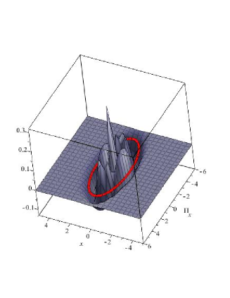
Figure 1: Wigner function for third excited state, $n=3$, ($M_{p}=\frac{1}{2\pi}$). The corresponding classical trajectory is denoted by redline loci.

Let us define in the unconstrained phase space, the complex-valued holomorphic functions

$$\begin{cases}A=\sqrt{\frac{\omega M_{\textsc{p}}}{2}}(x+\frac{i\Pi_{x}}{\omega M_{\textsc{p}}}),\\ \bar{A}=\sqrt{\frac{\omega M_{\textsc{p}}}{2}}(x-\frac{i\Pi_{x}}{\omega M_{\textsc{p}}}).\\ \end{cases}$$ (43)

Then, classical Hamiltonian (31) will be

$$\mathcal{H}=\omega A\bar{A}-\mathcal{E}.$$ (44)

On the other hand, the Moyal commutation relation between these new variables is

$$[A,\bar{A}]_{\ast_{\textsc{m}}}=A\ast_{\textsc{m}}\bar{A}-\bar{A}\ast_{\textsc{m}}A=1,$$ (45)

where the Moyal star product is redefined as $\ast_{\textsc{m}}:=e^{\frac{1}{2}\left(\overleftarrow{\partial_{A}}\overrightarrow{\partial_{\bar{A}}}-\overleftarrow{\partial_{\bar{A}}}\overrightarrow{\partial_{A}}\right)}$ hirshfeld . The Moyal star product between $A$ and $\bar{A}$ leads us to the following relation between star and ordinary products of holomorphic variables

$$\bar{A}\ast_{\textsc{m}}A=\bar{A}e^{\frac{1}{2}\left(\overleftarrow{\partial_{A}}\overrightarrow{\partial_{\bar{A}}}-\overleftarrow{\partial_{\bar{A}}}\overrightarrow{\partial_{A}}\right)}A=\bar{A}A-\frac{1}{2}.$$ (46)

Consequently, by combining Eq. (46) and Eq. (44) we obtain the Hamiltonian for the model as

$$\mathcal{H}=\omega(\bar{A}*_{\textsc{m}}A+\frac{1}{2})-\mathcal{E.}$$ (47)

In addition, the Wigner function (40), in terms of the holomorphic variables will be

$$W_{n}(A,\bar{A})=\frac{1}{n!}(\bar{A})^{n}\ast_{\textsc{m}}W_{0}\ast_{\textsc{m}}(A)^{n},$$ (48)

where $W_{0}=2e^{-2A\bar{A}}$ denotes the ground state of the WF. Note that for the ground state we have $A\ast_{\textsc{m}}{W}_{0}=0=W_{0}\ast_{\textsc{m}}\bar{A}$. Now, the MWDW Eq. (37) will be

$$\begin{array}[]{cc}\mathcal{H}*_{\textsc{m}}W_{n}=\omega(\bar{A}*_{\textsc{m}}A+\frac{1}{2}-\mathcal{E})*_{\textsc{m}}W_{n}\\ =\left[\omega(n+\frac{1}{2})-\mathcal{E}\right]W_{n}=0,\end{array}$$ (51)

which leads to

$$\mathcal{E}_{n}=\omega(n+\frac{1}{2}).$$ (52)

III.1 Cosmological holographic principle in a radiation dominated universe

Let us first assume that the universe is radiation dominated, where $M=0$. In this case, Eq. (52) and definition of $\mathcal{E}$ in (27) give

$${\mathcal{N}}_{\gamma}=n+\frac{1}{2}.$$ (53)

As was mentioned at the beginning of this section, $\mathcal{N}_{\gamma}$ could be related to the total entropy of radiation. Recalling the relation of the energy density of radiation $\rho_{\gamma}$, the entropy density ${s_{\gamma}}$ and the scale factor ${a}$ with temperature, $\rho_{\gamma}=\frac{\pi^{2}}{30}gT^{4}$, $s_{\gamma}=\frac{4}{3}\frac{\rho}{T}$, $a(t)\sim\frac{1}{T}$ mukhan , and using these relations in definition of ${\mathcal{N}}_{\gamma}$ in (28), we find

$$\mathcal{N}_{\gamma}=\left(\frac{5\times 3^{5}}{2^{8}\pi^{4}g}\right)^{\frac{1}{3}}(S_{\gamma})^{\frac{4}{3}},$$ (54)

where $S_{\gamma}=2\pi^{2}a^{3}s_{\gamma}$ denotes the total entropy and $g$ is the internal degrees of freedom. Now, by inserting (53) into Eq. (54), we obtain

$$S_{\gamma}=\left(\frac{2^{8}\pi^{4}g}{5\times 3^{5}}\right)^{\frac{1}{4}}\left(n+\frac{1}{2}\right)^{\frac{3}{4}},$$ (55)

which shows that the total entropy of radiation is quantized. Let us now deal with the relation between the total entropy and the phase space average of the apparent horizon. First note that in definition (25), for a radiation dominated universe, we have $x(t)=a(t)$. Hence Eq. (43) leads us to obtain the scale factor in terms of holomorphic variables $a(t)=\frac{1}{\sqrt{2M_{\textsc{p}}\omega}}(A+\bar{A})$. One can easily show that the phase space average of biquadratic scale factor is

$$\begin{array}[]{cc}\left\langle a^{4}\right\rangle=\frac{1}{4M_{\textsc{p}}^{2}\omega^{2}}\left\langle(A+\bar{A})^{4}\right\rangle\\ =\frac{3}{2M_{\textsc{p}}^{2}\omega^{2}}\left(n^{2}+n+\frac{1}{2}\right).\end{array}$$ (58)

On the other hand, the apparent horizon of a radiation dominated universe is given by, $R_{\text{ah}}^{2}=(\mathrm{H}^{2}+\frac{1}{a^{2}})^{-1}={\frac{6\pi^{2}M^{2}_{\textsc{p}}}{\mathcal{N}_{\gamma}}}a^{4}$, where ${H}$ is the Hubble parameter. Therefore the phase space average of the area for the apparent horizon becomes

$$\langle\mathcal{A}_{\text{ah}}\rangle:=4\pi\langle R^{2}_{\text{ah}}\rangle=\frac{L^{2}_{\textsc{p}}}{4\pi}\left(1+\frac{n^{2}}{n+\frac{1}{2}}\right),$$ (59)

where $L_{\textsc{p}}$ is the reduced Planck’s length. Hence, the phase space average of the apparent horizon is quantized. By comparing Eqs. (55) and (59) for large values of the quantum number $n$ we obtain

$$S_{\gamma}\simeq g^{\frac{1}{4}}\left(\frac{\langle\mathcal{A}_{\text{ah}}\rangle}{4G}\right)^{\frac{3}{4}}.$$ (60)

The above equation is in the form conjectured by ’t Hooft 't Hooft1 .

III.2 ’t Hooft conjecture in a dust dominated universe

Let us now return to a universe filled only with dust, (${\mathcal{N}_{\gamma}}=0$). In this case, comparing Eqs. (27) and (52) implies the following quantization rule for the total mass of the universe

$$M=\sqrt{24\pi^{2}(n+\frac{1}{2})}M_{\textsc{p}}.$$ (61)

We now estimate the total entropy of the dust dominated universe. Consider the case where a system has a total of $\Omega$ states of equal likelihood. Then the entropy will be

$$S=\ln(\Omega),\hskip 8.5359pt(k_{\text{B}}=1).$$ (62)

Further, let us assume that all the particles are identical. Then $\Omega=\tilde{n}^{N}$, where $\tilde{n}$ is the number of states accessible to a single particle, hence

$$S=N\ln(\tilde{n}).$$ (63)

Evaluating the one particle phase space, one finds kittel for an ideal gas with $N$ free particles

$$S_{(\text{ideal})}=N\ln\left(\frac{V}{N}(\frac{\text{m}T}{2\pi})^{\frac{3}{2}}e^{\frac{5}{2}}\right),$$ (64)

where $V$ is the volume and $m$ denotes the mass of particles. For the case of a continuous fluid, let us rewrite Eq. (64). To this end, we consider an ideal gas contained within a small volume element $dV$. The number of particles inside $dV$ is

$$dN=\frac{\rho}{\text{m}}dV.$$ (65)

Inserting expression (65) into Eq. (64), the entropy associated with the volume element, in terms of the density of the fluid, can be written as

$$dS^{(\text{dust})}=\frac{\rho}{\text{m}}\ln\left(\frac{KT^{\frac{3}{2}}}{\rho}\right)dV,$$ (66)

where $K=(\frac{m^{5}e^{5}}{2\pi})^{\frac{1}{2}}$ gron . For a dust dominated universe, the density and temperature are $\rho=\rho_{0}(\frac{a}{a_{0}})^{-3}$ and $T=T_{0}(\frac{a}{a_{0}})^{-2}$. Hence we have $S^{(\text{dust})}=\ln(KT^{\frac{3}{2}}_{0}/\rho_{0})N$. We use the simple approximation

$$S^{(\text{dust})}\simeq N=\frac{M}{\text{m}},$$ (67)

which is accurate within two orders of magnitude because, as noted by Fermi, all large logs are less than a thousand even in cosmology. Therefore from Eqs. (61) and (67) we obtain

$$S_{n}^{(\text{dust})}\simeq\frac{M_{\textsc{P}}}{\text{m}}\pi\sqrt{24(n+\frac{1}{2})}.$$ (68)

Let us investigate ’t Hooft conjecture for this model. The apparent horizon of a dust dominated universe using the definition of total mass in Eq. (28) and the Friedmann equation is given by

$$R^{2}_{\text{ah}}=\frac{6\pi^{2}M_{\textsc{P}}^{2}}{M}a^{3}.$$ (69)

Moreover, using definition (10), the phase space average of the cubic scale factor will be

$$\begin{array}[]{cc}\left\langle a^{3}\right\rangle=\left\langle(x-x_{0})^{3}\right\rangle=\\ \left\langle x^{3}\right\rangle-3x_{{}_{0}}\left\langle x^{2}\right\rangle+3x^{2}_{0}\left\langle x\right\rangle-x^{3}_{0},\end{array}$$ (72)

where from definition (43) we have $x=\frac{1}{\sqrt{2\omega M_{\textsc{p}}}}(A+\bar{A})$. Hence, with an eye on the definition of $x_{0}$ in (25), we obtain

$$\left\langle a^{3}\right\rangle=\frac{3M(n+\frac{1}{2})}{M^{2}_{\textsc{p}}\omega^{2}}+\left(\frac{M}{M_{\textsc{p}}\omega}\right)^{3}.$$ (73)

Eqs. (61) and (73) lead us to

$$\left\langle a^{3}\right\rangle=\frac{5\sqrt{2}}{({M_{\textsc{p}}\omega})^{\frac{3}{2}}}\left({n+\frac{1}{2}}\right)^{\frac{3}{2}}.$$ (74)

Therefore, the phase space average of squared apparent horizon becomes $\left\langle R^{2}_{\text{ah}}\right\rangle=\left(\frac{30\pi^{2}}{\omega^{2}}\right)\left(n+\frac{1}{2}\right)$, which shows that the area of the apparent horizon is quantized

$$\left\langle\mathcal{A}_{\text{ah}}\right\rangle=4\pi\left\langle R^{2}_{\text{ah}}\right\rangle=\left(\frac{5L^{2}_{\textsc{p}}}{6\pi}\right)\left(n+\frac{1}{2}\right).$$ (75)

Furthermore, from Eqs. (61) and (75) the total mass of the universe is

$${M}=M_{\textsc{p}}\frac{12\pi}{\sqrt{10}}\left(\frac{\langle\mathcal{A}_{\text{ah}}\rangle}{4G}\right)^{\frac{1}{2}}.$$ (76)

Substituting (76) into (67), the entropy of dust will be

$$S^{(\text{dust})}\simeq\frac{M_{\textsc{p}}}{m}\left(\frac{\langle\mathcal{A}_{\text{ah}}\rangle}{4G}\right)^{\frac{1}{2}}.$$ (77)

For further simplification, we use the well known relation between the radius of universe (herein the radius of apparent horizon defined via $L_{\text{ah}}:=\sqrt{\langle\mathcal{A}_{\text{ah}}\rangle}/4\pi$) and mass of nucleons, $m$, as a result of the uncertainty principle Sivaram

$$L_{\text{ah}}\simeq\sqrt{N}\frac{1}{m}=\sqrt{\frac{M}{m}}\frac{1}{m}.$$ (78)

By substituting Eqs. (61) and (75) in Eq. (78) we obtain

$$m\simeq M_{\text{P}}(n+\frac{1}{2})^{-\frac{1}{6}}.$$ (79)

Also combining Eqs. (75), (77) and (79) we obtain

$$S^{(\text{dust})}\simeq\left(\frac{\langle\mathcal{A}_{\text{ah}}\rangle}{4G}\right)^{\frac{2}{3}},$$ (80)

which again is in agreement with ’t Hooft conjecture. Let us investigate this result for large values of quantum number $n$, which according to the correspondence principle, the behavior of the model should reduce to its corresponding classical region. For very large values of $n$, we can estimate from relation (55) the following value for the entropy of radiation

$$S_{\gamma}\simeq n^{\frac{3}{4}}.$$ (81)

On the other hand, the entropy of the dust content of the universe will be

$$S^{(\text{dust})}\simeq n^{\frac{2}{3}}.$$ (82)

Let us examine our model for present epoch of the universe. The current entropy density of radiation in the universe is $s_{0\gamma}=2970(\frac{T_{0}}{2.5K})^{3}\frac{1}{\text{cm}^{3}}$. Therefore, the entropy of radiation is $S_{0\gamma}\simeq 10^{88}$. This estimation leads us to obtain the approximate value of the quantum number $n$ as $n\simeq 10^{117}$. Hence by inserting the obtained value of the quantum number $n$ in Eq. (82), we obtain $S^{(\text{dust})}\simeq 10^{79}$. This is in agreement with the classical estimation of the entropy of dust in the universe farmpton . At the end of this section, let us concentrate on the relation of our simple quantum cosmology model with the Large Number Hypothesis (LNH). For very large values of quantum number $n$, Eqs. (61), (75) and (79) simplify to the following well known scaling relations

$$\begin{cases}M\simeq\beta^{3}M_{\text{P}},\\ L_{\text{ah}}\simeq\beta^{3}L_{\text{P}},\\ m\simeq\beta^{-1}M_{\text{P}},\end{cases}$$ (83)

where $\beta:=n^{1/6}\simeq 10^{19}$. As showed by Marugan and Carneiro LNH , the scaling relations that lie behind the LNH can be expressed in the same way as the above relations. Also, they have shown that if one assumes a flat universe dominated by the cosmological constant $\Lambda$, then Dirac’s LNH can be explained in terms of the holographic conjecture. On the other hand, our results show that the CHP could be the result of quantum nature of the universe. Consequently it seems to be natural that the LNH could be embedded in quantum cosmology as one can see in relations (83). Eliminating $\beta$ from the two last scaling relations in (83), we obtain

$$m\simeq\left(\frac{1}{GL_{\text{ah}}}\right)^{\frac{1}{3}},$$ (84)

This equation is equivalent to the empirical Weinberg formula for the mass of the pion Weinberg .

IV Conclusion

In this paper we studied the deformation quantization or phase space quantization of a closed quantum FLRW model, whose matter is either a fluid of radiation or dust. Our results show that the peaks of the WF coincides with the classical trajectory of the universe. Our main upshot is that the CHP can be achieved by means of quantization of cosmological models. According to the CHP the entropy of non-black hole configurations is given by relation $S\simeq(\frac{\mathcal{A}}{4G})^{\frac{3}{4}}$, where ${\mathcal{A}}$ denotes the area of containing volume. We showed that the same result is maintained for radiation dominated universe, where ${\mathcal{A}}$ is replaced by the phase space average of apparent horizon $\langle{\mathcal{A}}_{\text{ah}}\rangle$, and $S$ is the total entropy (inside and outside). On the other hand, for a dust dominated universe, we obtained $S\simeq(\frac{\langle\mathcal{A_{\text{ah}}}\rangle}{4G})^{\frac{2}{3}}$. It seems that the power of apparent horizon in units of Planck’s surface is different for various matter configurations: for black holes this value is equal to 1, for radiation it is equal to 3/4, and for dust it is equal to 2/3. We are aware that our results are obtained within a very simple cosmological model. Nevertheless, we think they are intriguing and provide motivation for subsequent research works. Possible extensions to test the CHP may include

• Considering various Bianchi cosmological models.

• Considering other perfect fluids besides radiation and dust.

• Exploring the modified theories of gravity, like string cosmology and $f(R)$ theories.

V Acknowledgments

The authors would like to thank the anonymous referee for enlightening comments.

References

• (1) J. Moyal, Proc. Cambridge Philos. Soc. 45, 99 (1949).
• (2) H. Weyl, Z. Phys. 46, 1 (1927), E. Wigner, Phys. Rev. 40, 749 (1932), H. J. Groenewold, Physica 12, 405 (1946), F. Bayen, M.  Flato, C. Fronsdal, A. Lichnerowicz and D. Sternheimer, Ann. of Phys., 111, 111 (1978), A. Groenewold, Physica 12, 405 (1964).
• (3) P. Tillman, arXiv:gr-qc/0610159.
• (4) M. Kontsevich, Lett. Math. Phys. 48, 35 (1999).
• (5) A.C. Hirschfeld and P. Henselder, Am. J. Phys. 70, 5 ( 2002).
• (6) M Hillery, R.F. Oconnell, M.C. Scully and E.P. Wigner, Phys. Rep. 106, 121 (1984), T. Curtright, D. Fairlie and C. Zachos, Phys. Rev. D 58, 025002 (1998), M. Levanda and V. Fleurov, Ann. Phys. (N.Y.) 292, 199 (2001), C. Zachos, Int. J. Mod. Phys. A 17, 297 (2002).
• (7) T. Curtright, T. Uematsu and C. Zachos, J. Math. Phys. 42, 2396 (2001), F. Bonneau, M. Gerstenhaber, A. Giaquinto and D. Sternheimer, J. Math. Phys. 45, 3703 (2004), C. Zachos, Int. J. Mod. Phys. A, 17, 297 (2002).
• (8) H. Weyl, Group Theory and Quantum Mechanics. Dover, New York (1931).
• (9) B. Fedosov, J. Diff. Geom. 40, 213 (1994), M. Gadella, Prog. Phys., 43, 229 (1995).
• (10) J. V. Neumann, Math. Ann. 104 (1931) 570.
• (11) G. ’t Hooft, arXiv:gr-qc/9310026.
• (12) S. Leonard, J. Math. Phys. 36, 6377 (1995).
• (13) A.K. Biswas, J. Maharana and R.K. Pradhan, Phys. Lett. B 462, 243 (1999), G. Veneziano, Phys. Lett. B 454, 22 (1999).
• (14) M. Maggiore and A. Riotto, Nucl. Phys. B 548, 427 (1999).
• (15) S. Kalyana Rama and T. Sarkar, Phys. Lett. B 450 55 (1999).
• (16) W. Fischler and L. Susskind, arXiv:hep-th/9806039.
• (17) R. Easther and D. Lowe, Phys. Rev. Lett. 82, 4967 (1999).
• (18) D. Bak and S.J. Rey, Class. Quant. Grav. 17, 83 (2000).
• (19) S.W. Hawking and G.F.R. Ellis, The Large Scale Structure of Space-Time. Cambridge University Press, Cambridge, (1973).
• (20) S. Jalalzadeh and P.V. Moniz, Phys. Rev. D 89, 083504, (2014).
• (21) V. Mukhanov, Physical Foundations of Cosmology. Cambridge University Press, Cambridge, UK (2005).
• (22) R. Cordero, H. Garcia-Compean and F.J. Turrubiates, Phys. Rev. D 83, 125030 (2011).
• (23) C. Kittel and G. Kroemer, Thermal Physics. Freeman, W. H. (1980), 2nd ed.
• (24) M. Amarzguioui and O. Grøn, Phys. Rev. D 71, 083011 (2005).
• (25) P. Frampton, S.D.H. Hsu, T.W. Kephart and D. Reeb, Class. Quant. Grav. 26, 145005 (2009).
• (26) R. Bousso and S.W. Hawking, Phys. Rev. D 54, 6312 (1996), J. Garriga and A. Vilenkin, Phys. Rev. D 56, 2464 (1997), A.D. Linde, Phys. Rev. D 58, 083514 (1998).
• (27) C. Sivaram, Astrophys. Sp. Sci., 124, 195 (1986).
• (28) G. A. Mena Marugan and S. Carneiro, Phys. Rev. D 65, 087303 (2002).
• (29) S. Weinberg, Gravitation and Cosmology, Wiley, New York, (1972).