Region segmentation for sparse decompositions: better brain parcellations from rest fMRI

Abstract

Functional Magnetic Resonance Images acquired during resting-state provide information about the functional organization of the brain through measuring correlations between brain areas. Independent components analysis is the reference approach to estimate spatial components from weakly structured data such as brain signal time courses; each of these components may be referred to as a brain network and the whole set of components can be conceptualized as a brain functional atlas. Recently, new methods using a sparsity prior have emerged to deal with low signal-to-noise ratio data. However, even when using sophisticated priors, the results may not be very sparse and most often do not separate the spatial components into brain regions. This work presents post-processing techniques that automatically sparsify brain maps and separate regions properly using geometric operations, and compares these techniques according to faithfulness to data and stability metrics. In particular, among threshold-based approaches, hysteresis thresholding and random walker segmentation, the latter improves significantly the stability of both dense and sparse models.

1 Introduction

Functional connectivity between brain networks observed during resting state functional Magnetic Resonance Imaging (R-fMRI) is a promising source of diagnostic biomarkers, as it can be measured on impaired subjects such as stroke patients [9]. However, its quantification highly depends on the choice of the brain atlas. A brain atlas should be i) consistent with neuroscientific knowledge ii) as faithful as possible to the original data and iii) robust to inter-subject variability.

Publicly available atlases (such as structural [8] or functional [13] atlases) went through a quality assessment process and are reliable. To extract a data driven atlas from R-fMRI, Independent Component Analysis (ICA) remains the reference method. In particular, it yields some additional flexibility to adapt the number of regions to the amount of information available. Networks extracted by ICA are full-brain and require a post-processing step to extract the salient features, i.e., brain regions, which is often done manually [5] (see figure 4). To avoid post-processing and directly extract regions, more sophisticated approaches rely on sparse, spatially-structured priors [1]. Indeed, maps of functional networks or regions display a small number of non-zero voxels, and thus are well characterized through a sparsity criterion, even in the case of ICA [11, 3]. However, sophisticated priors such as structured sparsity come with computational cost and still fail to split some networks into separate regions. Altogether, region extraction is unavoidable to go from brain image decompositions to Regions-of-Interest-based analysis [6].

A simple approach to obtain sharper maps is to use hard thresholding, which is a good sparse, albeit non convex, recovery method [2]. We improve upon it by introducing richer post-processing strategies with spatial models, to avoid small spurious regions and isolate each salient feature in a dedicated region. Based on purely geometric properties, these take advantage of the spatially-structured and sparsity-inducing penalties of recent dictionary learning methods to isolate regions. These can also be used in the framework of computationally cheaper ICA algorithms. In addition to these automatic methods that extract brain atlases, we propose two metrics to quantitatively compare them and determine the best one. The paper is organized as follows. In section 2, we introduce the region extraction methods. Section 3 presents the experiments run to compare them. Finally, results are presented in section 4.

2 Region extraction methods

Extracting regions to outline objects is a well-known problem in computer vision. For the particular problem of extracting regions of interest (ROIs) out of brain maps, we want a method that i) handles 3D images ii) processes one image while taking into account the remainder of the atlas (e.g., region extraction for a given image may be different depending on the number of other regions) and iii) isolates each salient feature from a smooth image in an individual ROI without strong edges or structure (see figure 1). Here, we assume that a given set of brain maps has been obtained by a multivariate decomposition technique.

Most of the following methods allow overlapping components after region extraction. In fact, multivariate decomposition techniques most often decompose the signal of one voxel as a linear mixture of several signal components. In practice, these overlapping regions are small and located in areas of low confidence. Voxels that belong to no component are left unlabeled.

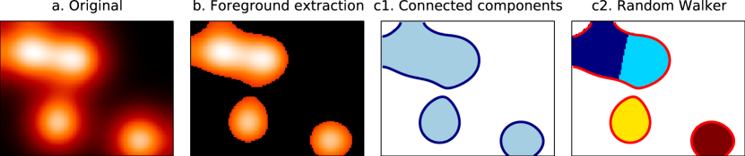
Figure 1: Example of region extraction. Foreground pixels (b) are extracted from the original image (a). Regions are extracted using connected component extraction (c1) or random walker (c2).

2.1 Foreground extraction

Let $\mathcal{I}=\{I_{1},...,I_{k}\}$ be a set of brain maps (3D images), or atlas. $I(p)$ designates the value for image $I$ at point $p$. We define by $\mathcal{F}(I)$ the set of foreground points of image $I$, i.e., the points that are eligible for region extraction. We propose two strategies to extract the foreground.

Hard assignment.

Hard assignment transforms a set of maps into a brain segmentation with no overlap between regions. That means that each voxel will be represented by a unique brain map from the atlas. This map is the one that has the highest value for this voxel. The result is a segmentation from which we can extract connected components.

$$\mathcal{F}_{hard}(I_{i})=\{p\in I_{i}\;|\;\text{argmax}_{j\in[1,k]}\,I_{i}(p)=i\}$$

Automatic thresholding.

Thresholding is the common approach used to extract ROIs from ICA. However, the threshold is usually set manually and is different for each map. In order to propose an automatic threshold choice, we consider that on average, an atlas assigns each voxel to one region. For this purpose, we set the threshold $t^{k}(\mathcal{I})$ so that the number of nonzero voxels corresponds to the number of voxels in the brain:

$$\mathcal{F}_{automatic}(I_{a})=\{p\in I_{a},I(p)>t^{k}(\mathcal{I})\}$$

2.2 Component extraction

Connected components.

Let $\mathcal{N}(p)$ be the set of neighbors of point $p$. Two points $p_{1}$ and $p_{n}$ are $\mathcal{N}$-connected if $p_{n}$ can be reached from $p_{1}$ by following a path of consecutive neighboring points:

$$(p_{1},p_{n})\;\mathcal{N}\text{-connected}\equiv\exists(p_{2},...,p_{n-1}):p_{i+1}\in\mathcal{N}(p_{i}),\forall\ i\in[1,n-1]$$

We define a connected component as a maximum set of foreground points that are $\mathcal{N}$-connected. The set of all $\mathcal{N}$-connected components for a given image $I$ (see figure 1.c1) is written $ccs(\mathcal{N},I)$. Extraction of connected components can be done after hard assignment or automatic thresholding to obtain ROIs (figures 2 and 4). In the following methods, we consider the points extracted with automatic thresholding as foreground ($\mathcal{F}=\mathcal{F}_{automatic}$) and use more sophisticated priors to extract ROI.

Hysteresis thresholding.

Hysteresis thresholding is a two-threshold method where all voxels with value higher than a given threshold $t_{high}$ are used as seeds for the regions. Neighboring voxels with values between the high threshold $t_{high}$ and the low threshold $t_{low}$ are added to these seed regions. In our setting, the high threshold can be seen as a minimal activation value over the regions in order to sort out regions of marginal importance. Each brain map has its own optimal value but, in practice, cross validation has shown that keeping the 10% highest foreground voxels as seeds gives the best results. The automatic thresholding strategy described above is used to set the low threshold $t_{low}$.

Conserving connected components that have their maximum value over $t_{high}$ is done at component extraction:

$$ccs_{hysteresis}(\mathcal{N},I)=\{c\in ccs(\mathcal{N},I)\;|\;\text{max}(c)\geq t_{high}\}$$

Random Walker.

Random Walker is a seed-based segmentation algorithm similar to watershed. It calculates, for each point $p$, the probabilities to end up in each of the seeds by doing a random walk across the image starting from $p$. The original version of the algorithm [4] was of probabilistic nature, whereby the probability to jump to a neighboring point is driven by the gradient magnitude between them. After convergence the point is attached to the seed with the highest probability.

Random Walker can also be seen as a diffusion process. It is equivalent to hysteresis thresholding where regions that have grown enough to share a boundary are not allowed to be merged. The probabilities to reach each of the seeds can be computed using the laplacian matrix of the graph associated with the map. Due to space limitations we refer the reader to [4] for the complete description of the algorithm. We suppose $seed(p)$ returns the seed associated with point $p$. We refine our neighborhood relationship by considering two points as neighbours only if they are associated to the same seed:

$$\mathcal{N}_{rw}(p)=\{q\in\mathcal{N},seed(p)=seed(q)\}\;;\;ccs_{rw}(I)=ccs(\mathcal{N}_{rw},I)$$

Note that, in our setting, a high value in the map means a high confidence. So, instead of using the finite difference gradient, we consider the max of the image minus the lowest voxel. Therefore, diffusion is facilitated in areas of high confidence and more difficult elsewhere. We take the local maxima of the smoothed image as seeds for the algorithm.

3 Experiments

Experiments are made on a subset of the publicly available Autism Brain Imaging Database Exchange dataset. Preprocessing is done with SPM and includes slice timing, realignment, coregistration to the MNI template and normalization. We select 101 subjects suffering from autism spectrum disorders and 93 typical controls from 4 sites and compute brain atlases on 10 cross-validation iterations by taking a random half of the dataset as the train set. We extract regions from these atlases and quantify their performance on the other half of the dataset with two metrics.

We investigate two decomposition methods to extract brain maps from resting-state fMRI: ICA –independent component analysis– that yields full brain continuous maps, and MSDL –multi-subject dictionary learning–, [1], that directly imposes sparsity and structure on the maps thanks to the joint effect of $\ell_{1}$ norm and total variation minimization. Our goal is to compare the effects of region extraction on sparse and non-sparse sets of maps.

To quantify the usefulness of a set of regions extracted automatically, we consider metrics that characterize two different aspects of the segmentation: the ability to explain newly observed data and the reproducibility of the information extracted, as in the NPAIRS framework [7]. We use Explained Variance (EV) to measure how faithful the extracted regions are to unseen data. Stability with regards to inter-subject variability is measured using Normalized Mutual Information (NMI) over models learned on disjoint subsets of subjects.

Following [10], we extract $k=42$ maps. For the metrics to be comparable, we need to apply them on models of similar complexity, i.e. with the same number of regions. For this purpose, we assume that there must be on average 2 symmetric regions per map (some of them may have more, and some of them may have only one inter-hemispheric region). We therefore aim at extracting 2$k$ regions, and take the largest connected components after region extraction. In the end, some maps may not contribute to the final atlas.

3.1 Data faithfulness – Explained variance

The explained variance measures how much a model accounts for the variance of the original data. The more variance is explained, the better the model explains the original data. Linear decomposition models original data $y_{orig}$ by decomposing them into two matrices. In our case, these matrices are brain networks $\mathcal{I}$ and their associated time series $y_{model}$. Time series of regions are measured using least square fitting instead of simple averaging to handle mixed features in region overlaps. Explained variance of these series is then computed over the original ones.

$$y_{orig}=\mathcal{I}\times y_{model}+y_{\varepsilon}\;;\;\text{EV}(y_{model})=1-\frac{\text{Var}(y_{\varepsilon})}{\text{Var}(y_{orig})}=\frac{\text{Var}(y_{orig})-\text{Var}(y_{model})}{\text{Var}(y_{orig})}$$

3.2 Stability – Normalized Mutual Information

To assess model stability, we rely on Normalized Mutual Information, a standard clustering similarity score, applied on hard assignments [12]: given two hard assignments $U$ and $V$ with marginal entropy $H(U)$ and $H(V)$ respectively,

$$NMI(U,V)=\frac{H(U)+H(V)-H(U,V)}{\sqrt{H(U)*H(V)}}\;;H(X)=-\sum_{i=1}^{n}p(x_{i})\;log\;p(x_{i})$$

4 Results

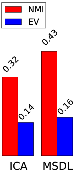
a. Hard thresholding

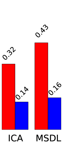
b. Automatic thresholding

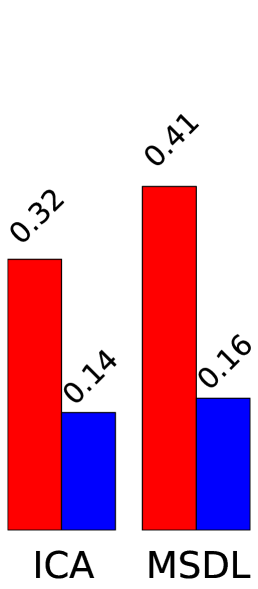
c. Hysteresis thresholding

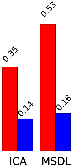
d. Random Walker

Figure 2: Comparison of region extraction methods (after selection of 2$k$ regions). Brain maps obtained with MSDL are located on the left. The activated regions are symbolically represented below in a height map. The bars on the right of each image represent the Normalized Mutual Information and Explained variance obtained on dense maps (ICA) and sparse maps (MSDL). Random walker is the most stable method.

Visual cortex
Original Manual Hard Automatic Hysteresis Random Walker
Default mode network
Original Hard Automatic Hysteresis Random Walker

Figure 2 presents region extraction results using each method on the same map. In all figures, the threshold applied during region extraction is shown in a given slice to help understanding. Results for each metric are displayed on the right. We vary parameters for each model (smoothing for ICA, 3 parameters of MSDL) and, for each region extraction method, display the best 10% results across parametrization. Figure 4 shows 2 networks out of 42 extracted.

Region shape

The regions extracted by hard assignment (figure 2.a) present salient angles and their limits do not follow a contour line of the original map. The straight lines are the results of two maps in competition with each other. The 1D cut shows that the threshold applied when using hard thresholding is not uniform on the whole image. The other methods look smoother and follow actual contour lines of the original map. On this particular example, automatic thresholding (figure 2.b) extracts 2 regions: a large one on the left and a very small one on the right. This is one of the drawbacks of thresholding: small regions can appear when their highest value is right above the threshold. Thanks to its high threshold, hysteresis thresholding (figure 2.c) gets rid of the spurious regions but still fails to separate the large region on the left. Random Walker (figure 2.d) manages to split the large region into two subregions.

Similarly, in figure 4 we can see that Random Walker manages to split the default mode network into 3 components, where other methods extract two.

Stability.

Random Walker dominates the stability metric. It uses local maxima to get regions seeds, and will thus split regions even if they are connected after thresholding. Its performance is statistically significant for both dense and sparse atlases and any parametrization. The stability improvement is larger for sparse than for dense maps. This could be due to the inability of random walker to compensate for the original instabilities of the models.

Data fidelity.

The explained variance scores on best performing models, shown in figure 2, are similar for all methods. In poorly performing models, we observe that automatic and hysteresis thresholdings are slightly above random walker (about 2%), exhibiting the same trade-off as in [1].

5 Discussion and conclusion

Functional atlases extracted using ICA or sparse decomposition methods are composed of continuous maps and sometimes fail to separate symmetric functional regions.

Starting from hard thresholding [2], we introduce richer strategies integrating spatial models, to avoid small spurious regions and isolate each salient feature in a dedicated region. Indeed, the notion of regions is hard to express with convex penalties. Relaxations such as total-variation used in [1] only captures it partially, while a non-convex segmentation step easily enforces regions. We find that a Random-Walker based strategy brings substantial increase in stability of the regions extracted, while keeping very good explanatory power on unseen data. Finer results and interpretation may arise by using more adapted metrics, for example a version of DICE that can deal with overlapping fuzzy regions. This point is under investigation.

Acknowledgments We acknowledge funding from the NiConnect project and NIDA R21 DA034954, SUBSample project from the DIGITEO Institute, France.

References

- [1] Abraham, A., Dohmatob, E., Thirion, B., Samaras, D., Varoquaux, G.: Extracting brain regions from rest fMRI with total-variation constrained dictionary learning. In: MICCAI, p. 607 (2013)
- [2] Blumensath, T., Davies, M.E.: Iterative hard thresholding for compressed sensing. Applied and Computational Harmonic Analysis 27, 265 (2009)
- [3] Daubechies, I., Roussos, E., Takerkart, S., Benharrosh, M., Golden, C., D’Ardenne, K., Richter, W., Cohen, J.D., Haxby, J.: Independent component analysis for brain fMRI does not select for independence. Proc Natl Acad Sci 106, 10415 (2009)
- [4] Grady, L.: Random walks for image segmentation. Pattern Analysis and Machine Intelligence, IEEE Transactions on 28(11), 1768–1783 (2006)
- [5] Kiviniemi, V., Starck, T., Remes, J., et al.: Functional segmentation of the brain cortex using high model order group PICA. Hum Brain Map 30, 3865 (2009)
- [6] Nieto-Castanon, A., Ghosh, S.S., Tourville, J.A., Guenther, F.H.: Region of interest based analysis of functional imaging data. Neuroimage 19, 1303 (2003)
- [7] Strother, S., Anderson, J., Hansen, L., Kjems, U., Kustra, R., Sidtis, J., Frutiger, S., Muley, S., LaConte, S., Rottenberg, D.: The quantitative evaluation of functional neuroimaging experiments: the NPAIRS data analysis framework. NeuroImage 15, 747 (2002)
- [8] Tzourio-Mazoyer, N., Landeau, B., Papathanassiou, D., Crivello, F., Etard, O., Delcroix, N., Mazoyer, B., Joliot, M.: Automated anatomical labeling of activations in SPM using a macroscopic anatomical parcellation of the MNI MRI single-subject brain. Neuroimage 15, 273 (2002)
- [9] Varoquaux, G., Baronnet, F., Kleinschmidt, A., Fillard, P., Thirion, B.: Detection of brain functional-connectivity difference in post-stroke patients using group-level covariance modeling. In: MICCAI, pp. 200–208 (2010)
- [10] Varoquaux, G., Gramfort, A., Pedregosa, F., Michel, V., Thirion, B.: Multi-subject dictionary learning to segment an atlas of brain spontaneous activity. In: Inf Proc Med Imag. pp. 562–573 (2011)
- [11] Varoquaux, G., Keller, M., Poline, J., Ciuciu, P., Thirion, B.: ICA-based sparse features recovery from fMRI datasets. In: ISBI. p. 1177 (2010)
- [12] Vinh, N., Epps, J., Bailey, J.: Information theoretic measures for clusterings comparison: Variants, properties, normalization and correction for chance. Journal of Machine Learning Research 11, 2837–2854 (2010)
- [13] Yeo, B., Krienen, F., Sepulcre, J., Sabuncu, M., et al.: The organization of the human cerebral cortex estimated by intrinsic functional connectivity. J Neurophysio 106, 1125 (2011)