The Effect of Network-Topology to Propagation on Networks

Abstract

We study the effect of the network topology to propagation phenomena on networks in this article. We do not assume any propagation model such as the contact process or SIR model[1] because the study is only the consideratons of the purely topological effect, especially the effect of cycles of a network. To uncover universal properties independent of explicit propagation models is expected due to it. First of all, we introduce some indeces for propagation phenomena of a network. Second we introduce a concept of cycles with a little differences to usal cycles, which is called ”STOC” in the body of this article. We find some analytic relations between thesm, STOC and some indeces. Moreover we can find the total number of STOCs in a network, analytically. This consideration leads to an extension of the celebrated ”Euler’s polyhedron formula”, which is only applicable to planar graphs. This extended formula is applicable to any graphs. Last we estimate numerically the indeces and the number of STOCs based on the theoretical considerations for some complex networks and make some discussion on the effects of cycles in networks to propagation.

Keywords;Small world network, Scale free network, topology, cycle, propagation, Eurer’s Polyhedron Theorem

1 Introduction

In 1967, Milgram has made a great impact on the world by advocating ”Six Degrees of Separation”[2]. After that, his research group makes some social experiments to establish the conjecture[3], [4]. Recently Watts and his research group adduced evidence in support of it more intensively by experiments using e-mail[5], [6].

We have studied the mathematical structures of complex networks [7]-[11] to understand ”six degrees of separation” advocated by Milgram[2]. Especially, we have developed an original formulation [7]-[11] based on ” string formulation” developed by Aoyama[12] in order to study the effect of cycles in a network to propagation.

We have proceeded with our study for scale free networks and small world networks in the basis of Milgram condition proposed by Aoyama [12]. As a result, it proved that the generalized clustering coefficient, which takes on the responsibility of cycles in a network, has the opposite effect for propagation in the both networks. That is, the existence of closed paths in a network impedes the propagation in small world networks, but does not in scale free networks[7]-[11]. An epitom is given in Fig.1. The analyses in the articles, however, did no more than the study up to cycles with 6 nodes.

So changing the approach to this problem, we develop arguments from a new angle, that is an ego-network inspired by [13], on this problem. We also study propagation phenomena on networks from purely topological point of view, especially the effect of cycles of a network. Thus we do not assume any propagation models such as the contact process or SIR model[1]. First of all, we introduce some indeces for propagation phenomena of a network, which is easy to estimate. Second we introduce a concept of cycles with a little differences to usal cycles, called ”STOC”. We find some relations between STOC and the indeces, and one among them is represented by a recursion relation for regular networks. This recursion relation is solvable analytically so that the solution gives an explict relation between STOC and the indeces. Thanks to the recursion relation, we also can evaluate the total number of STOC in a network that leads to an extension of the celebrated ”Euler’s polyhedron formula”, which is only applicable to planar graphs. Last we estimate numerically the indeces and the number of STOCs based on the theoretical considerations for some complex networks and make some discussions on the effects of cycles in networks to propagation.

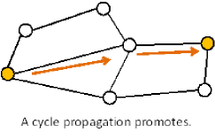
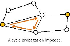
Figure 1: Two roles of cycle structure on a graph.

2 Indeces for propagation

We first introduce a generation number of nodes. We choose a node freely. This node is $0$-th generation node. We call the $n$-generation node that can arrive at the $0$-th generation node by shortest $n$-hops. Thus the number of nodes of the first generation is the same as the degree $k_{0}$ of the $0$-th generation node. For example of Fig.2 where $v_{1}$ is the $0$-th generation node, $v_{2}$ and $v_{3}$ are first generation nodes and $v_{4}$, $v_{5}$ and $v_{6}$ are second generation nodes, respectively.

Though we should properly consider a rate of propagation to adjacent nodes in introducing indeces for propagation, we here introduce rather simple indeces, since our aim is to uncover the purely topological effect to the propagation on networks. Indeces introduced in this article represent how many nodes the nodes at a certain generation can arrive. Thus the indeces in this article represent the maximum number of nodes that nodes at every generation can reach by one hop. It would be natural that these indeces give an estimation of propagation. When the starting node is $v_{i}$, we define the local absolute index $N_{M}(v_{i})$ of $M$-generation by the number of nodes that newly reaches by $M$-th hop from $v_{i}$. In Fig.2 Cwhen $v_{1}$is the starting node, we find $N_{0}(v_{1})=1$, $N_{1}(v_{1})=3$ and $N_{2}(v_{1})=2$, where the index introduced depends on the starting node. We further introduce the absolute index $N_{M}$ independently of a starting node as the average over all starting nodes;

$$N_{M}=\frac{1}{N}\sum_{i=1}^{N}N_{M}(v_{i}),$$ (1)

where $N$ is the total number of nodes in the considering network. These indeces means the maximum number of nodes that can propagate from a generation to the next generation. The expected value of the absolute index also gives the average length from a starting node $v_{i}$ to nodes in a whole network. So the index gives the detail for an average length.

Moreover we define the local relative index $R_{M}(v_{i})$ of $M$-generation by the ratio between the local absolute index for $M$-th generation and the one for $(M+1)$-th generation;

$$R_{M}(v_{i})=\frac{{N}_{M+1}(v_{i})}{{N}_{M}(v_{i})}.$$ (2)

The correspondong relative index $R_{M}$ is defined by the average over all starting nodes;

$$R_{M}=\frac{1}{N}\sum_{i=1}^{N}R_{M}(v_{i}).$$ (3)

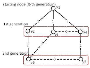
Figure 2: The generation number of nodes and edges

3 Definition of STOC

We define the generation number of edges. We define $n$-th generation edge as the set of edges that connect a $(n-1)$-th generation nodes to a $(n-1)$-th or a $n$-th generation nodes. The figures on edges show the generation number of edges in Fig.2.

Next we define the primary edges that are edges connecting $n$-th generation nodes and $(n+1)$-th generation nodes, where anyone among the edges is the primary edge but others are secondary edges in the cases that plural $n$-th generation nodes connect a $(n+1)$-th generation node. Edges that connect among nodes in the same generation are also defined as secondary edges. Solid lines are primary edges and dotted lines are secondary ones in Fig.2.

We define STOC as cycles that include only one secondary edge. A cycle $v1-v4-v3-v1$ is STOC consisting of three nodes in Fig.2, since the cycles includes only one secondary edge. Cycles $v1-v2-v6-v3-v1$ and $v1-v2-v6-v4-v3-v1$ are likewise STOCs with four nodes and five nodes, respectively. The cycle $v4-v3-v6-v5-v4$, however, is not STOC, since it includes two secondary nodes.

STOC is a concept that removes redundancy in usual cycles in a sense. STOCs that newly is made by introducing $M$-th generation edges are called $M$-generation STOCs. $C^{(j)}_{M}(v_{i})$ represents the number of $M$-generation STOCs with node $j$ when the starting node is $v_{i}$. The numbers of $M$-th generation STOCs with any nodes are written as $C_{M}(v_{i})=(C^{(3)}_{M},C^{(4)}_{M}(v_{i}),\cdots,C^{(j)}_{M}(v_{i}),\cdots,C^{(2M)}_{M}(v_{i}))$, where $2M\geq j\geq 3$, because there are no cycles with nodes less than 3 and there are only cycles with at most $2M$ nodes up to $M$-th genetartion node. In Fig.2 Cwe find $C_{0}(v_{1})=(0),\;C_{1}(v_{1})=(0,0),\;C_{2}(v_{1})=(1,1,0,0),\;C_{3}(v_{1})=(0,0,1,0,0,0)$.

4 Relations between the indeces and STOC

4.1 The absolute index and STOC

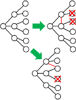
Figure 3: Relations between cycles and propagation

The local absolute index in every generation becomes maximum at a tree like structure in a network as shown in the left figure of Fig.3. When there are some cycles, as shown in the above figure to the right of Fig.3, the number of nodes in the next generation decreases by two every cycle with odd number nodes. Moreover when a cycle with even number nodes is made, the number of nodes in the next generation and the further next generation decreases by one as is shown in the lower right network in Fig.3, respectively. From these considerations, we can obtain the following relation between the absolute index $N_{M}(v_{i})$ and STOC for $M\geq 2$.

$$N_{M}(v_{i}) = \sum_{j=1}^{N_{M}-1}\bigl{(}k^{j}_{M-1}(v_{i})-1\bigr{)}-2\sum_{i=3,5\cdots}^{2M-1}C^{(i)}_{M}(v_{i})$$ (4)

$$- \sum_{i=4,6\cdots}^{2M}C^{(i)}_{M}(v_{i})-\sum_{i=4,6\cdots}^{2(M-1)}C^{(i)}_{M-1}(v_{i}),$$

where $k^{j}_{M-1}(v_{i})$ is the degree of $j$-th node in $M-1$ generation. It can be proven that (LABEL:120 does not depend on which edges is secondary edges. The proof is omitted in this article because of limited page space. The essential fact for the proof is that one secondary corresponds to just one cycle. The first term of the right hand side in (4) represents the contribution to $N_{M}$ at tree approximation of a network. The second term and the third term of right hand side represent the decreasing numbers of nodes in the present generation when cycles with odd number of nodes and even number of nodes are made, respectively. The fourth term represents the decreasing numbers of nodes in the present generation when a cycle with the even number of nodes is made at two generations before. (4) is actually confirmed with some regural networks, a ring-type network, extended rings, the triangular lattice, tetragonal lattice and the tetragonal lattice on torus.

When the degree of all nodes included in the network is equal to constant $k$, we obtain

$$N_{M}(v_{i}) = N^{(k)}_{M-1}(v_{i})(k-1)-2\sum_{i=3,5\cdots}^{2M-1}C^{(i)}_{M}(v_{i})$$ (5)

$$- \sum_{i=4,6\cdots}^{2M}C^{(i)}_{M}(v_{i})-\sum_{i=4,6\cdots}^{2(M-1)}C^{(i)}_{M-1}(v_{i}).$$

(4) is a recursion relation for the local absolute index. We can analytically solve the recursion relation;

$$N_{M}(v_{i}) =k(k-1)^{M-1}$$ (6)

$$- \sum_{j=2}^{M}\Bigl{(}2\sum_{i=j}^{M}(k-1)^{M-i}C^{(2j-1)}_{i}(v_{i})$$

$$+k \sum_{i=j}^{M-1}(\!k\!-\!1\!)^{M\!-\!1\!-\!i}C^{(2j)}_{i}(v_{i})+C^{(2j)}_{M}(v_{i})\Bigr{)}.$$

(6) can be proven by mathematical induction and also applies for $M=1$. Thus we could indicate the relation between the local absolute index $N^{(k)}_{M}$ and the number of STOCs by (6). It is considered that STOC impedes propagation on the whole from (6) in networks with the same degree for every node. STOCs with the odd number of nodes and STOCs with the even number of ones have a different type effect on the impediment of the propagation.

4.2 Total number of STOCs and Euler’s polyhedron theorem

It is also possible to find the total number of STOCs in the whole network from (4). Let $L$ be the last generation for nodes in a network, so there are no nodes in $L+1$ generation. Taking the sum from $0$-th generation to $L$-th generation for (4), we obatin

$$\sum_{i=0}^{L}N_{i} = \sum_{i=0}^{L}N_{i}+N_{L}=2+\sum_{i=0}^{L-1}(\overline{k_{i_{j}}}-1)N_{i}$$ (7)

$$-2\sum_{i=2}^{L}\sum_{j=3}^{2i}C^{(j)}_{i}+\sum_{i=4,6,8\cdots}^{2L}C^{(i)}_{L+1},$$

The third term in the right hand side of (8) shows the total number of STOCs. We must manage the last term in the right hand side of (8) in order to obtain the total number of STOCs without any other information about STOCs.

When there are $L$-th generation nodes, there are, however, $L+1$ generation edges. We formally consider $(L+1)$-th generation as a dummy in order to include $L+1$ generation edege. As is shown later, this device solve the problem for the last term. Thus taking the sum from $0$-th generation to $(L+1)$-th generation, we obatin

$$\sum_{i=0}^{L+1}N_{i} = \sum_{i=0}^{L}N_{i}+N_{L+1}=2+\sum_{i=0}^{L}(\overline{k_{i_{j}}}-1)N_{i}$$ (8)

$$-2\sum_{i=2}^{L+1}\sum_{j=3}^{2i}C^{(j)}_{i}+\sum_{i=4,6,8\cdots}^{2(L+1)}C^{(i)}_{L+1},$$

where $\overline{k_{i_{j}}}$ is the number of edges between the nodes in $(i-1)$-th generation and $j$-th node in $i$-th generation. The second term in the right hand side in (8) is just the total number of STOCs in a whole network. The last term of the right hand side in (8) vanishes, since there is no STOC with odd numbers of nodes in the $L+1$-th generation. Thus we obtain the total number of STOCs

$$S_{L}(v_{i}) = \sum_{i=2}^{L}\sum_{j=3}^{2i}C^{(j)}_{i}\!(v_{i})\!$$ (9)

$$= 1+\frac{1}{2}\sum_{i=0}^{L}N_{i}\overline{k_{i_{j}}}-\sum_{i=0}^{M}N_{i}.$$

The fact is, this formula is applicable not only to the last generation $L$, but also to every generation $M$ by simirarly thinking some dummies at every generation. Thus we can estimate the total number $S_{M}(v_{i})$ of STOCs upto any generations, where $\overline{k_{i_{j}}}$ is numerically calculated in actuality.

Further we find that the (9) leads to an exatension of the celebrated Euler’s polyhedron theorem (without genuses) at the last generation, because the second term and the third term of the right hand side in (9) means the total number of edges and nodes in a whole network, respectively;

$$Euler:surface = 1+edges-nodes,$$ (10)

$$STOC:S_{M}(v_{i}) = 1+edges-nodes,$$ (11)

where (10) applies when one surface on the outside of a network is omitted and $S_{M}(v_{i})$ in (11) does not depend on any starting node $v_{i}$, because it is determined only by the total numbers of the surfaces and the edges in the considering network. While the Euler’s polyhedron theorem applies only to planar graphs, (11) applies in any graphs. Thus when we put up a menbrane at one STOC, (11) gives an exatension of the Euler’s polyhedron theorem.

5 Simulation and its results

We numerically calculate the number of STOCs and the absolute index in every generation in two types of complex networks to consider their relations. One is the small world network proposed by Watts-Strogatz[14] where the probability $p$ replacing edges is a control parameter for the number of small size cycles. Second is the scale free network proposed by Holme-Kim[15] where $q$, the probability making cycles consist of three nodes, plays role of a control parameter for the number of small size cycles. The network becomes Barabasi-Albert model[16] with scaling exponent $3$ at $q=0$. We set up the network size $N=3000$ and the average deggree $<k>=6$ in both networks. The number of STOCs in every generation is estimated by taking a difference of two adjacent generations in (9) and the average over all starting nodes $v_{i}$. Ten times of average are taken at every simulation. The total number of STOCs has not any effect on propagation phenomena, since it is determined by the total number of nodes and edges in a network by the extended Euler’s polyhedron theorem. We will show only the results of the absolute indeces in this article, since the relative indces are essentially the same behaviors as the absolute ones in both networks.

5.1 Small World Network

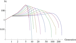
Figure 4: The absolute index of small world network

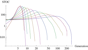
Figure 5: STOC of small world network

In the small world network, $p$ is changed from 0 to 1 by $p=2^{-m}$ for $m=0,1,2,\cdots 10$. The absolute index and the total number of STOCs of small world network are given by Fig.4 and Fig.5. Each curved line in Fig.4 and Fig.5 shows the results of 11 kinds of $p$, where the curved line with the smallest maximum is one for the smallest $p$ and the one with the largest maximum is the one for $p=1.0$ in the both figures. These show that Fig.4 behaves the same way as Fig.5. While from Fig.4, one can reach many nodes in small generation at large $p$, one can reach many nodes in large generation at small $p$.

5.2 Holme-Kim Network

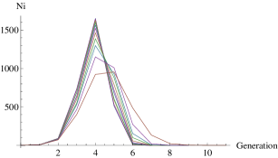
Figure 6: The absolute index of Holme-Kim model

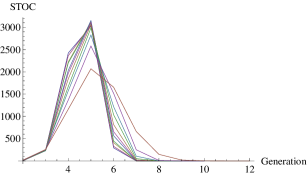
Figure 7: STOC of Holme-Kim model

$q$ is moved from 0 to 1 at 0.1 intervals. The absolute index and the total number of STOCs of Holme-Kim network are given by Fig.6 and Fig.7. Each curved line in Fig.6 and Fig.7 shows the results of 11 kinds of $q$, where the curved line with the smallest maximum is one for the smallest $q=0$ and the one with the largest maximum is the one for $q=1.0$. These show that Fig.6 behaves the same way as Fig.7. While from Fig. 6, one can reach many nodes in small generation at large $q$, one can reach many nodes in relatively large generation at small $q$.

5.3 Small World Network vs. Holme-Kim network

Comparing the results in the both networks, the maxmum of $N_{i}$ in Holme-Kim model is larger than the one of Small-world networks. We find that there is a generation reachable to many nodes of the next generation in Holme-Kim model. The fact is consistent with the well-known fact that Holme-Kim model is more smallnes than Watts-Strogatz mode[13].

From these four figures, we find that the number of STOCs reach the peak, after the absolute indeces reach the peak in bothy networks. We guess that the reason is because edges between the same generation are also likely drawn after many nodes are connected in a generation. We can check that the total numbers of STOCS are consistent with the extended Euler’s polyhedron theorem. From these numerical analyses, we resulted in the conclusion that STOC is an important concept for studying propagation phenomena on networks.

6 Concluding remarks

In this research, we can succeed in making a connection with cycles with any sizes, where cycles with only six size have been discussed till now, and propagation on a network by introducing new indeces for propagation and STOCs that is a new concept of the cycles.

Moreover we showed that the total number of STOCs leads to an exatension of the celebrated Euler’s polyhedron theorem where surfaces are considered as menbranes put up at every STOC. Thus the extended theorm applies to non-planar graph. The constant $1$ appeared in (10 is essentially a topological constant. It is important problem that the constant $1$ appeared in (11 has aany topological meanings.

We calculated indeces and the number of STOC in every generation in some typical complex networks. As result, we find that the behaviors of the indeces for propagation are totally different in scale free networks and Watts-Strogatz[14]-type small world network. So a series of the absolute indeces $N_{M}$ or the relative indeces $R_{M}$ may give an index characterizing various type networks. For it, it is needed to study more diverse networks. The total number of STOCs has not any effect on propagation in networks, because it is given by the extended Euler’s theorem, independently of details of network topology. We, however, resulted in the conclusion that STOC in every generation plays an important role of propagation phenomena on networks.

References

- [1] W. O. Kermack and A. G. McKendrick, gA Contribution to the Mathematical Theory of Epidemics, hProc. Roy. Soc. of London. Series A, Vol. 115, No. 772 (Aug. 1, 1927), pp. 700-721
- [2] S. Milgram, ”The small world problem”, Psychology Today 2, 60-67 (1967)
- [3] J. Travers and S. Milgram, ”An Experimental Study of the Small World Problem”, Sociometry 32, 425 (1969)
- [4] C. Korte and S. Milgram, ”Acquaintance links between White and Negro populations: Application of the small world method”, Journal of Personality and social Psychology 15 (2), pp.101-108 (1970)
- [5] D. J. Watts et al., Small World Project-Columbia University. http://small world.columbia.edu/
-
[6]
P.S.Dodds, R.Muhamad and D.J. Watts, ”An Experimental Study of Research in Global
Social Networks”, Science 301, pp.827-829:
http://small world.columbia.edu/images/dodds2003 pa.pdf (2003) - [7] N. Toyota, IEICE Thecnical Report, ”String Formalism for -Clustering Coefficient-Toward Six Degrees of Separations”,NLP2009-49(2009) in Japanese.
- [8] N. Toyota, ” -th Clustering coefficients and Adjacent Matrix for Networks: Formulation based on String”, arXiv:0912.2807
- [9] N. Toyota and T. Sakamoto, ”- degrees of separation in the string-adjacent matrix formalism”, sixth symposium of network ecology, 2009 Dec. in Japanese
- [10] N. Toyota and T. Sakamoto, ”Six degrees of separation and the generalized clustering coefficients in scale free networks ”, 42-th lecture meeting of the Society of Instrument and Control Engineers in Hokkaido, 2010.Feb. in Japanese
- [11] Norihito Toyota, gp-th Clustering coefficients and q-th degrees of separation based on String-Adjacent Formulation h CPreprint arXiv:1002.3431
- [12] H. Aoyama, ”Six degrees of separation; some caluculation”, SGC library65, ” Introduction to Network Science”, (2008) ; H, Aoyama, Y.Fujiwara, H, Ietomi, Y. Ikeda and W.Soma ”EconoPhysics”,Kyouritu Shuppan 2008 in Japanese
- [13] M.E.J.Newman, gEgo-centered Networks and the ripple effect or why all your friends are wired h, Social Networks 25, p.83;arXiv. Cond-mat/0111070 ,2003.
- [14] D. Watts, S. Strogatz, ”Collective dynamics of small-world networks”, Nature 393 1998.
- [15] P.Holme and J.Kim, gGrowing Scale-Free Networks with Tunable Clustering h,Phys. Rev. E65 ,026107;arxiv;cond-mat/0110452,2002.
- [16] A.-L.Barabasi, and R.Albert, ”Emergence of scaling in random networks”, Science 286, pp. 509-512 ,1999 D