Exploring the structure and function of temporal networks with dynamic graphlets

Abstract

With the growing amount of available temporal real-world network data, an important question is how to efficiently study these data. One can simply model a temporal network as either a single aggregate static network, or as a series of time-specific snapshots, each of which is an aggregate static network over the corresponding time window. The advantage of modeling the temporal data in these two ways is that one can use existing well established methods for static network analysis to study the resulting aggregate network(s). However, doing so loses valuable temporal information either completely (in the first case) or at the interface between the different snapshots (in the second case). Here, we develop a novel approach for studying temporal network data more explicitly, by using the snapshot-based representation but by also directly capturing relationships between the different snapshots. We base our methodology on the well established notion of graphlets (subgraphs), which have been successfully used in numerous contexts in static network research. Here, we take the notion of static graphlets to the next level and develop new theory needed to allow for graphlet-based analysis of temporal networks. Our new notion of dynamic graphlets is quite different than existing approaches for dynamic network analysis that are based on temporal motifs (statistically significant subgraphs). Namely, these approaches suffer from many limitations. For example, they can only deal with subgraph structures of limited complexity. Also, their major drawback is that their results heavily depend on the choice of a null network model that is required to evaluate the significance of a subgraph. However, choosing an appropriate null network model is a non-trivial task. Our dynamic graphlet approach overcomes the limitations of the existing temporal motif-based approaches. At the same time, when we thoroughly evaluate the ability of our new approach to characterize the structure and function of an entire temporal network or of individual nodes, we find that the dynamic graphlet approach outperforms the static graphlet approach, independent on whether static graphlets are applied to the aggregate network or to the snapshot-based network representation. Clearly, accounting for more temporal information helps with result accuracy.

I Introduction

I-A Motivation

Networks (or graphs) are powerful models for studying complex systems in various domains, from biological cells to societies to the Internet. Traditionally, due to limitations of data collection techniques, researchers have mostly focused on studying the static network representation of a given system [1]. However, many real-world systems are not static but they change over time [2]. With new technological advancements, it has become possible to record temporal changes in network structure (or topology). Thus, on top of the traditional static network representation of the system of interest, one can now also obtain information on arrival or departure times of nodes or edges. Examples of temporal networks include person-to-person communication [3], online social [4], citation [5], cellular [6], and functional brain [7] networks.

The increasing availability of temporal real-world network data, while opening new opportunities, has also raised new challenges for researchers. Namely, despite a large arsenal of powerful methods that already exist for studying static networks, these methods cannot be directly applied to temporal network data. Instead, the simplest approach to deal with a temporal network is to completely discard its time dimension by aggregating all nodes and edges from the temporal data into a single static network. While this would allow to directly apply to the resulting aggregate network the existing and well established methods for static network analysis, such an aggregate or static approach loses all important temporal information from the data. To overcome this, one could model the temporal network as a series of snapshots, each of which is a static network that aggregates the temporal data observed during the corresponding time interval. Then, with such a snapshot-based network representation, one could use a static-temporal approach to study each snapshot independently via the existing methods for static network analysis and then consider time-series of the results. However, this strategy treats each network snapshot in isolation and discards relationships between the different snapshots. Clearly, both static and static-temporal approaches overlook temporal information that is important for studying evolution of a dynamic system [2]. Therefore, proper analysis of temporal network data requires development of conceptually novel strategies that can fully exploit the available temporal information from the data. And this is exactly the focus of our study.

I-B Related work

Static networks. One way to study the structure of a static network is to compute its global properties such as the degree distribution, diameter, or clustering coefficient [1]. However, even though global network properties can summarize the structure of the entire network in a computationally efficient manner, they are not sensitive enough to capture detailed topological characteristics of the complex real-world networks [8]. Thus, local properties have been proposed that can capture more detailed aspects of complex network structure. For example, one can study small partial subgraphs called network motifs that are statistically significantly over-represented in a network compared to some null model [9, 10]. However, the practical usefulness of network motifs has been questioned, since the choice of null model can significantly affect the results [11, 8], and since selecting an appropriate null model is not a trivial task [12]. Hence, to address this challenge, graphlets have been proposed [13], which are small induced subgraphs of a network that can be employed without reference to a null model (Figure 1), unlike network motifs. Also, unlike network motifs, graphlets must be induced subgraphs, whereas motifs are partial subgraphs, which makes graphlets more precise measures of network topology compared to motifs [8]. Graphlets have been well established when studying static networks. For example, they were used as a basis for designing topologically constraining measures of network [13] or node [14] similarities. These measures in turn have been used to develop state-of-the-art algorithms for various computational problems such as network alignment [15, 16, 17], clustering [18, 19], or de-noising [20], as well as for a number of application problems, such as studying human aging [21, 22], cancer [23, 24], or pathogenicity [18, 25].

Temporal networks. Analogous to studying static networks from a global perspective, temporal networks can also be studied by considering evolution of their global properties [5, 26]. As this again leads to imprecise insights into network changes with time, recent focus has shifted onto local-level dynamic network analysis via notion of “temporal motifs”. In the simplest case of the static-temporal approach, static motifs (as defined above) are counted in each snapshot and then their counts are compared across the snapshots [27]. To overcome this approach’s limitation of ignoring any motif relationships between different snapshots, the notion of static network motifs has been extended into several notions of temporal motifs [28, 29, 30, 31, 32]. However, each of these existing temporal motif-based approaches suffers from at least three of the following drawbacks:

1. They can only deal with motif structures of limited complexity, such as small motifs or simple topologies (e.g., linear paths) [28, 29, 32], which limits their practical usefulness to capture complex network structure in detail.

2. They pose additional constraints, such as limiting the number of events (temporal edges) a node can participate in at a given time point [30, 31].

3. They allow for obtaining the motif-based topological “signature” of the entire network only but not of each individual node [27, 28, 29, 32, 30, 31], whereas the latter is very useful when aiming to link the network topological position of a node to its function via e.g., network alignment or clustering (see the above discussion on static graphlets).

4. Importantly, just as static motifs, the temporal motif-based approaches rely on a null model [27, 28, 29, 32, 30, 31], which again makes their practical usefuleness questionable [11, 8, 12], especially since adequately choosing an appropriate null model is an even more complex problem in the dynamic setting compared to the static setting (see above).

5. They are typically dealing with directed networks (e.g., mobile communications). While this is not necessarily a drawback per se, many real-world networks are undirected (e.g., protein-protein interaction networks). Thus, these approaches cannot be directly applied to such networks.

Analogous to extending the notion of network motifs from the static to dynamic setting, recently, we took the first step to do the same with the notion of graphlets. Namely, we used graphlets, along with several other measures of network topology, as a basis of a static-temporal approach to study human aging from protein-protein interaction networks [21]. That is, we counted static graphlets, along with the other network measures, within each snapshot (where different snapshots correspond to different human ages), and then we studied the time-series of the results to gain insights into network structural changes with age [21]. However, in this initial work, we only used the already established notion of static graphlets within a static-temporal approach that ignored important relationships between different snapshots, in order to demonstrate that accounting for at least some temporal information in the static-temporal fashion can improve results compared to using the trivial static (aggregate) approach that has traditionally been used in the field of computational biology. Further important temporal inter-snapshot information remains to be explored via a novel truly temporal approach. In this study, we aim to develop such an approach, as follows.

I-C Our contribution

To overcome the issues of the existing methods for temporal network analysis, we take the well established notion of static graphlets to the next level to develop new theory of dynamic graphlets that are needed for efficient truly temporal network analysis. Unlike any of the existing temporal motif-based approaches, our dynamic graphlets allow for all of the following: 1) they can study topological and temporal structures of arbitrary complexity, as permitted by available computational resources; 2) there are no limitations such as the one on the number of events that a node can participate in; 3) they can capture the topological signature of the entire network as well as of each individual node; 4) they allow for studying temporal networks without relying on a null model; 5) they complement the temporal motif-based approaches by working with undirected networks. Unlike the existing graphlet-based static-temporal approach, our dynamic graphlets explicitly consider relationships between different snapshots.

Compared to the existing methods, the closest approaches to our work are those of temporal motifs as defined in [30], static graphlets [13, 14], and static-temporal graphlets [21]. Since temporal motifs have limitations (see above), the major one being dependence on a null model, they are not comparable to our dynamic graphlet approach. Static and static-temporal graphlet approaches, which ignore all temporal information or inter-snapshot temporal information, respectively, are directly comparable to our dynamic graphlet approach, which does account for inter-snapshot temporal information. Thus, our goal is to fairly compare the three approaches, in order to evaluate the effect on result accuracy of the amount of temporal information that the given approach can consider.

In the rest of the paper, we formally define our novel notion of dynamic graphlets and present an approach for enumerating all dynamic graphlets of an arbitrary size and counting them in a given network (Section II). We thoroughly evaluate the ability of dynamic graphlets to characterize the structure and function of an entire temporal network as well as of individual nodes. Namely, on both synthetic and real-world temporal network data, we measure how well our approach can group (or cluster) temporal networks (or nodes) of similar structure and function and separate those networks (or nodes) of dissimilar structure and function. We find that our dynamic graphlet approach outperforms both static and static-temporal graphlet approaches in all of these tasks (Section III). This confirms our hypothesis that accounting for more temporal information leads to better result accuracy. This in turn illustrates real-life relevance of our new dynamic graphlet methodology, especially because the amount of available temporal network data is expected to continue to grow across many domains.

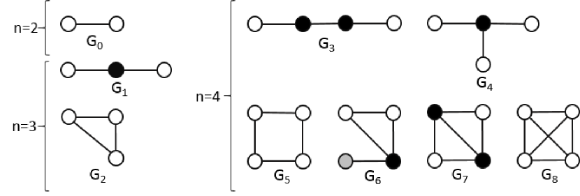
Figure 1: All nine static graphlets with up to four nodes, along with their 15 “node symmetry groups” (or formally, automorphism orbits) [13, 14]. Within a given graphlet, different orbits are denoted by different node colors. For example, there is a single orbit in graphlet $G_{2}$, as all three nodes are topologically identical to each other. But there are two orbits in graphlet $G_{2}$, as the two end nodes are topologically identical to each other but not to the middle node (and vice versa).

II Methods

We introduce the theoretic notion of dynamic graphlets in Section II-A. We give an algorithm for dynamic graphlet counting in Section II-B. We discuss a related notion of causal dynamic graphlets in Section II-C. We describe our experimental setup and evaluation framework in Section II-D.

II-A Dynamic graphlets

Let $G(V,E)$ be a temporal network, where $V$ is the set of nodes and $E$ is the set of events (temporal edges) that are associated with a start time and duration [2]. An event can be represented as a $4$-tuple $(u,v,t_{start},\sigma)$,where $u$ and $v$ are its endpoints, $t_{start}$ is its starting time, and $\sigma$ is its duration. Thus, each event is linked to a unique edge in the aggregate static network, whereas each static edge may be linked to multiple events. Note that here we consider undirected events, but most ideas can be extended to directed events as well.

Let $G^{\prime}(V^{\prime},E^{\prime})$ be a temporal subgraph of $G$ with $V^{\prime}\subseteq V$ and $E^{\prime}\subseteq E$, where $E^{\prime}$ is restricted to nodes in $V^{\prime}$. Let events $e_{i}$ and $e_{j}$ be $\Delta t$-adjacent if they share a node and if both events occur within a given time interval $\Delta t$. Two events $e_{i}$ and $e_{j}$ are $\Delta t$-connected if there exists a sequence of $\Delta t$-adjacent events joining $e_{i}$ an $e_{j}$. A temporal network is called $\Delta t$-connected if any two of its nodes are $\Delta t$-connected.

Let two nodes $s$ and $t$ be connected by a $\Delta t$-time-respecting path if there is a sequence of events $(v_{0},u_{0},t_{start0},\sigma_{0}),(v_{1},u_{1},t_{start1},\sigma_{1}),\dots,(v_{k},u_{k},t_{startk},\sigma_{k})$, such that $v_{0}=s$, $u_{k}=t$, $\forall i\in[0,k-1]$ $u_{i}=v_{i+1}$, and $t_{i+1}\in[t_{i}+\sigma_{i},t_{i}+\sigma_{i}+\Delta t]$. A temporal subgraph is $\Delta t$-causal if it has no isolated nodes and if for every two events in this subgraph there exists a $\Delta t$-time-respecting path containing both of the events. So, every $\Delta t$-causal subgraph is also $\Delta t$-connected, while the opposite is not always true.

Then, a dynamic graphlet is an equivalence class of isomorphic $\Delta t$-causal temporal subgraphs; equivalence is taken with respect to the relative temporal order of events. For isomorphism, we do not consider events’ actual start times but only their relative ordering. Thus, two $\Delta t$-causal temporal subgraphs will correspond to the same dynamic graphlet if they are isomorphic and their corresponding events occur in the same order. Note that we consider only $\Delta t$-causal temporal subgraphs, in contrast to temporal motifs that consider only $\Delta t$-connected subgraphs [30], so our definition is more restricting. Figure 2 illustrates all dynamic graphlets with up to three events, but we evaluate larger graphlets as well.

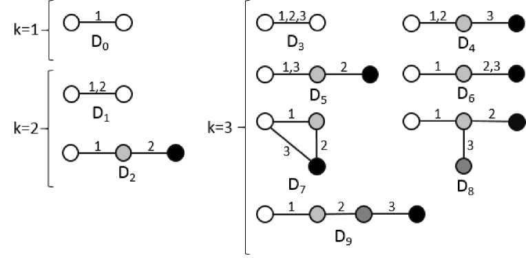
Figure 2: All dynamic graphlets with up to three events, along with their automorpism orbits. Multiple events along the same edge are separated with commas. Node colors correspond to different orbits.

Note that if for a given dynamic graphlet with $n$ nodes and $k$ events we discard the order of the events and remove duplicate events over the same edge, we get a static graphlet with $n$ nodes and $k^{\prime}\leq k$ edges, which we call the backbone of the dynamic graphlet. Each dynamic graphlet has a single backbone, while one backbone can correspond to different dynamic graphlets (Figure 3). Supplementary Table S1 shows for each static graphlet with up to five nodes [14] the number of corresponding dynamic graphlets with up to ten events.

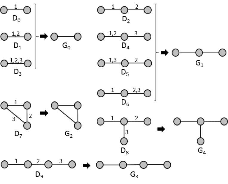
Figure 3: All dynamic graphlets $D_{i}$ with up to three events, and their corresponding (static) backbones $G_{j}$.

The above definitions allow us to describe all dynamic graphlets of a given size in the entire network, in order to obtain topological signature of the network. There already exists a popular notion of topological signature of an individual node in a static network, called the graphlet degree vector (GDV) the node, which describes the number of each of the static graphlets that the node “touches” at a specific “node symmetry group” (or automorphism orbit) within the given graphlet (Figure 1) [14]. Analogously, one might want to describe the node’s dynamic GDV equivalent. In this case, automorphism orbits of a dynamic graphlet will be determined based on both topological (as in static case) and temporal (unlike in static case) position of a node within the dynamic graphlet. Thus, a dynamic graphlet with $n>2$ nodes will have $n$ different orbits (Figure 2), whereas the number of orbits in a static graphlet of size $n$ is typically less than $n$ (Figure 1); note that for dynamic graphlets with $n=2$, there will be only one orbit, since events are undirected and thus their end nodes are topologically equivalent.

Next, we discuss the way for computing $D(n,k)$, the number of dynamic graphlets with $n$ nodes and $k$ events. Since at least $n-1$ edges are needed to connect $n$ nodes, it follows that $D(n,k)=0$ for $k<n-1$. Moreover, since we assume that events are undirected, $D(2,k)=1$, for any $k$. To compute $D(n,k)$ when $n\geq 3$ and $k\geq n-1$, notice that each dynamic graphlet with $k$ events can be formed from a dynamic graphlet with $k-1$ events and either $n-1$ or $n$ nodes, by adding a new event between some two existing nodes or between an existing node and a new node, respectively (Figure 4).

In the first case, we take a dynamic graphlet with $n$ nodes and $k-1$ events and add a new event between its existing nodes, in order to obtain a dynamic graphlet with $n$ nodes and $k$ events (e.g., construct $D_{6}$ from $D_{2}$). Due to the $\Delta t$-causality constraint, this new event has to involve at least one of the two nodes participating in event $(k-1)$. We can add the new event in $2n-3$ different ways: between one of these nodes and the “remaining” $n-2$ nodes (which is $2(n-2)=2n-4$ ways) or just duplicate event $(k-1)$.

In the second case, we take a dynamic graphlet with $n-1$ nodes and $k-1$ events and add an event from one of its nodes to the new ($n^{th}$) node, in order to obtain a dynamic graphlet with $n$ nodes and $k$ events (e.g., construct $D_{4}$ from $D_{1}$). For $n-1\geq 3$, there are two ways to do this, since there are two potential candidates for this new event (the two endpoints of event $(k-1)$). Note that since events are undirected, for $n-1=2$, the two nodes are indistinguishable from our point of view, and so we have only one way to construct a new dynamic graphlet with $3$ nodes and $k$ events.

In summary, we can get $2n-3$ new dynamic graphlets with $n$ nodes and $k$ events from each dynamic graphlet with $n$ nodes and $k-1$ events. Moreover, we can get two new dynamic graphlets with $n$ nodes and $k$ events from each dynamic graphlet with $n-1$ nodes and $k-1$ events. The only exception is for $n=3$, since we can get only one new dynamic graphlet with three nodes from a dynamic graphlet with two nodes, as these two nodes are indistinguishable (Figure 2). Importantly, since each dynamic graphlet with $k$ events has a unique $(k-1)$-“prefix” from which it was extended, all of these new dynamic graphlets with $n$ nodes will be different. Thus, we get the following recursive formulas for $D(n,k)$:

$$D(3,k)=3D(3,k-1)+D(2,k-1),n=3$$

$$D(n,k)=(2n-3)D(n,k-1)+2D(n-1,k-1),n>3$$

By expanding the formulas for few smallest values of $n$ and $k$, we can get the following closed-form solution:

$$D(n,k)=\sum\limits_{i=0}^{n-2}\frac{(-1)^{n+i}\binom{n-2}{i}(2i+1)^{k-1}}{2(n-2)!},n\geq 3.$$

Supplementary Table S2 shows dynamic graphlet counts for up to $n=11$ and $k=10$.

Since now we can compute $D(n,k)$, we next consider the task of enumerating and generating each of these dynamic graphlets (we discuss the process of counting each of the generated graphlets in Section II-B). We build upon the fact that each dynamic graphlet with $k$ events has a unique $(k-1)$-“prefix” (see above). Thus, we start with a single event (dynamic graphlet $D_{0}$ with $n=2$ and $k=1$) as the current graphlet and then recursively extend the current graphlet until the desired size is reached. Supplementary Algorithm S1 illustrates our enumeration procedure.

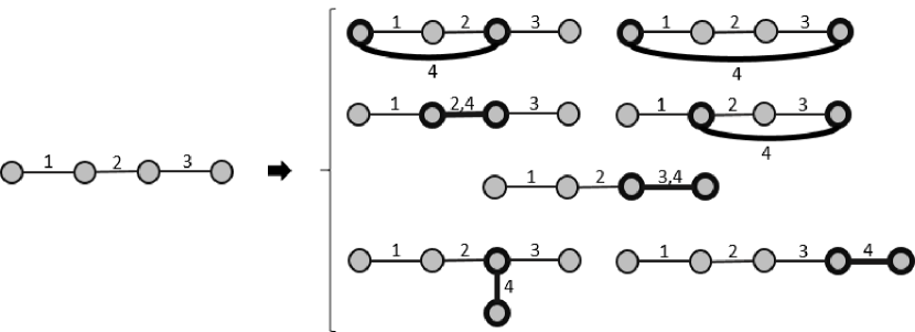
Figure 4: Illustration of how we extend a dynamic graphlet with an additional more recent event, on the example of $D_{9}$. There are seven possible extensions of $D_{9}$ (which contains four nodes and three events) with the most recent event $4$ (shown in bold) into a dynamic graphlet with four events. Five of the extensions keep the same number of nodes but increment the number of events, while the remaining two extensions increment both the number of nodes and events. Note that in order to extend $D_{9}$ with event $4$, at least one of the nodes involved in event $3$ has to participate in event $4$ as well.

II-B Counting dynamic graphlets in a network

As now we know the number of different dynamic graphlets with a given number of nodes and events and also how to enumerate and generate each one of them, how to actually count each of the dynamic graphlets in a given network?

We perform dynamic graphlet counting in the same way as we generate the graphlets. That is, for each event in a temporal network, we use this event as the current dynamic graphlet $D_{0}$ and then search for larger graphlets that are grown recursively from the current one (Figure 5). Supplementary Algorithms S2-S4 describe this algorithm. Its running time depends on the structure of the given temporal network. In general, since the algorithm explicitly goes through every dynamic graphlet that it counts, the running time is proportional to the number of dynamic graphlets. For a network with $D$ $\Delta t$-adjacent event pairs, counting all dynamic graphlets with up to $k$ events takes $\mathcal{O}(|E|+|E|(\frac{D}{|E|})^{k-1})$. As with static graphlets, the running time of exhaustive dynamic graphlet counting is exponential in graphlet size (but is still practical, as we will show). Yet, as elegant non-exhaustive approaches were proposed for faster static graphlet counting [33, 34], similar techniques can be sought for dynamic graphlet counting as well.

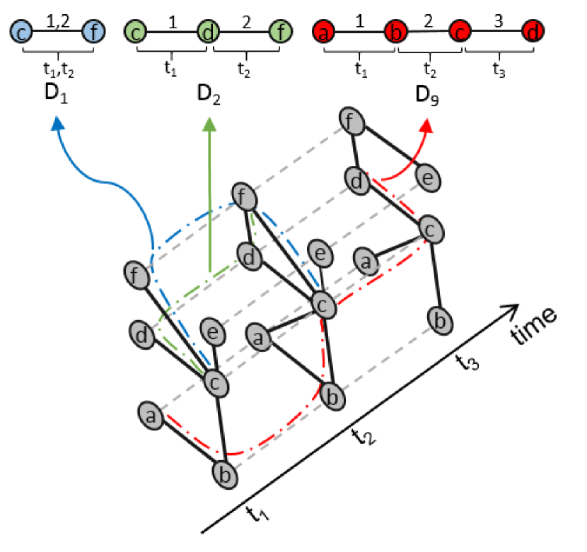
Figure 5: Illustration of our dynamic graphlet counting procedure. The temporal network is presented as a sequence of three snapshots. Dashed lines denote instances of the same node in different snapshots. Colored lines illustrate the path of how the temporal network is explored in order to count the given dynamic graphlet. Regular dynamic graphlet counting (Section II-B) will detect all three of the dynamic graphlets $D_{1}$ (involving nodes $c$ and $f$), $D_{2}$ (involving nodes $c$, $d$, and $f$), and $D_{9}$ (involving nodes $a$, $b$, $c$, and $d$). Causal dynamic graphlet counting (Section II-C) will detect only the first two of these dynamic graphlets. This is because nodes $c$ and $d$ are interacting in both the second and third snapshot, and thus, the third condition from the definition of causal dynamic graphlet counting is violated when it comes to $D_{9}$.

II-C Causal counting of dynamic graphlets in a network

A network having dense neighborhoods with many events between the same node pairs will have a large number of different dynamic graphlets with large counts. This is because for a given dynamic graphlet, there will be many $\Delta t$-adjacent candidates which can be used to “grow” this dynamic graphlet. For each of these possible extensions of a dynamic graphlet, we will again have many possibilities for further extension, and so on. For example, consider a snapshot-based network representation where each snapshot is the same dense graph. Clearly, a large number of different dynamic graphlets will be detected, yet many of them will just be artifacts of the consecutive snapshots “sharing” the dense network structure.

To address this issue and remove the likely redundant graphlet counts, which is expected to also reduce computational complexity of dynamic graphlet counting, we propose a modification to the counting process from Section II-B, as follows. When we are extending a dynamic graphlet ending with event $e_{1}=(u_{1},v_{1},t_{1},\sigma_{1})$ with a new event $e_{2}=(u_{2},v_{2},t_{2},\sigma_{2})$, if $\{u_{1},v_{1}\}=\{u_{2},v_{2}\}$, i.e., if the two events correspond to the same static edge, then we impose the same two conditions as in the regular counting procedure from Section II-B: 1) the two events $e_{1}$ and $e_{2}$ must be $\Delta t$-adjacent with $t_{2}>t_{1}$, and 2) the two events must share a node. Otherwise, if $\{u_{1},v_{1}\}\neq\{u_{2},v_{2}\}$, i.e., if the two events correspond to two different static edges, we also add a new third condition: to extend the dynamic graphlet ending with event $e_{1}$ with event $e_{2}$, $u_{2}$ and $v_{2}$ cannot interact between the starting times of $e_{1}$ and $e_{2}$ (i.e., $\not\exists e^{\prime}=(u_{2},v_{2},t^{\prime},\sigma^{\prime})\in E$ with $t_{1}-\sigma^{\prime}\leq t^{\prime}<t_{2}$).

Intuitively, the new third condition requires a “causal” relationship between $e_{1}$ and $e_{2}$: $u_{2}$ and $v_{2}$ start their interaction only after the end of $e_{1}$ (though note that there could still be an event involving $u_{2}$ and $v_{2}$ sometime before the start of $e_{1}$). That is, in order to extend a dynamic graphlet ending with event $e_{1}$ with some event $e_{2}$, the two nodes participating in $e_{2}$ should not interact with each other between the start of $e_{1}$ and the start of $e_{2}$, unless $e_{1}$ and $e_{2}$ involve the same nodes (otherwise, the counting process is as in Section II-B). This allows one to reduce the number of likely redundant temporal subgraphs that are being considered, which in turn reduced the total running time.

Note that we split the counting procedure into two above cases ($e_{1}$ and $e_{2}$ corresponding to the same static edge, and $e_{1}$ and $e_{2}$ not corresponding to the same edge) for the following reason. We want to impose the new third condition only in the latter case, but not in the former one. This is because in the former case we still want to allow for counting dynamic graphlets having consecutive repetitions of the same event, such as $D_{1}$ or $D_{4}$. And if we imposed the third condition in the former case as well, then such a dynamic graphlet would never be counted.

Henceforth, we refer to this modified counting procedure as causal dynamic graphlet counting. Figure 5 illustrates the distinction between regular and causal dynamic graphlet counting procedures. Clearly, causal dynamic graphlet counting allows for examining fewer dynamic graphlet options during counting compared to regular dynamic graphlet counting, because the former excludes from consideration graphlets that are likely artifacts of repeated events, unlike the latter. As a consequence, causal dynamic graphlet counting is expected to be more computationally efficient in terms of running time.

II-D Experimental setup

Graphlet methods under consideration, and the corresponding network construction strategies. We compare four graphlet-based approaches: static, static-temporal, dynamic and causal dynamic graphlets. To apply static graphlet counting to a temporal network, we first aggregate the temporal data into a single static network, by keeping the node set the same, and by adding an edge between two nodes in the static network if there are at least $w$ events between these two nodes in the temporal network. For other methods, we use a snapshot-based representation of the temporal network: we split the whole time interval of the temporal network into time windows of size $t_{w}$, and for each time window, we construct the corresponding static snapshot by aggregating the temporal data during this window with the parameter $w$, as above. For static and static-temporal graphlet approaches, we vary the number of graphlet nodes $n$, and for dynamic and causal dynamic graphlet approaches, we vary both the number of graphlet nodes $n$ and the number of graphlet events $k$.

We began our analysis by testing in detail $w$ values of 1, 2, 3, 5, and 10 on one of our data sets (see below). Since we observed no qualitative differences in results produced by the different choices of this parameter, we continued with the choice of $w=1$, and we report the corresponding results throughout the paper. We also tested multiple values for $t_{w}$ in each data set (see below), and again we saw no significant qualitative differences in the results. Hence, throughout the paper, we report results for $t_{w}=2$ (the unit of time for this parameter depends on the data set; see below).

Network classification. An approach that captures network structure (and function) well should be able to group together similar networks (i.e., networks from the same class) and separate dissimilar networks (i.e., networks from different classes) [35]. To evaluate our dynamic graphlet approach against static and static-temporal graphlet approaches in this context, we generate a set of synthetic (random graph) temporal networks of nine different classes corresponding to nine different versions of an established network evolution model [4]. We use synthetic temporal network data because obtaining real-world temporal network data for multiple different classes and with multiple examples per class is hard. And even if a wealth of temporal network data were available, we typically have no prior knowledge of which real-networks are (dis)similar, i.e., which networks belong to which functional class.

The network evolution model that we use was designed to simulate evolution of real-world (social) networks, and it incorporates the following parameters: node arrival rate, initiation of an edge by a node, and selection of edge destination. Specifically, the model is parameterized by the node arrival function $N(t)$ that corresponds to the number of nodes in the network at a given time, parameter $\lambda$ that controls the lifetime of a node, and parameters $\alpha$ and $\beta$ that control how active the nodes are in adding new edges. By choosing different options for the model parameters, we can generate networks with different evolution processes. In particular, for our analysis, we test three different types of the node arrival function (linear, quadratic, and exponential) and two sets of parameters corresponding to edge initiation ($\lambda_{1}=0.032$, $\alpha_{1}=0.8$, $\beta_{1}=0.002$, and $\lambda_{2}=0.02$, $\alpha_{2}=0.9$, $\beta_{2}=0.004$) [4], resulting in six different network classes. We also test a modification of the network evolution model, in which each node upon arrival simply adds a fixed number of edges (in our case, 20) according to preferential attachment and then stops [36]. Intuitively, this modification corresponds to preferential attachment model extended with a node arrival function. In this way, we create three additional network classes, one for each of the three node arrival functions, resulting in nine different network classes in total.

In order to test the robustness of the network classification methods to the network size, in each of the nine classes, we test three network sizes: 1000, 2000, and 3000 nodes. Then, for each network size and class, we generate 25 random graph instances. For the above synthetic network set, we report results for the following network construction parameters: $w=1$ and $t_{w}=2$. We tested other parameter values as well ($t_{w}=5$ and $t_{w}=10$), and all results were qualitatively similar. Also, unless otherwise noted, we report results for the largest network size of 3000 nodes. Results for the other network sizes were qualitatively similar.

Given the resulting aggregate or snapshot-based network representations, we then compute static, static-temporal, or dynamic graphlet counts in each network and reduce the dimensionality of the networks’ graphlet vectors with principle component analysis (PCA). For a given graphlet vector, we keep its first two PCA components, since in all cases the first two PCA components account for more than 90% of variation. Then, we use Euclidean distance in this PCA space as a network distance measure and evaluate whether networks from the same class are closer in the graphlet-based PCA space than networks from different classes, as described below.

Node classification. We also compare the three graphlet-based methods by evaluating whether they can group together similar nodes rather than entire networks. Specifically, we measure the ability of the methods to distinguish between functional node labels (i.e., classes) based on the nodes’ graphlet-based topological signatures. As a proof of concept, we do this on a publicly available Enron dataset [3], which is both temporal and contains node labels. Unfortunately, availability of additional temporal and labeled network data is very limited. The Enron network is based on email communications of 184 users from 2000 to 2002, and seven different user roles in the company are used as their labels: CEO, president, vice president, director, managing director, manager, and employee.

For the above real-world network, we report results for the following network construction parameters: $w=1$ and $t_{w}=2$ months. Note that we tested other parameter values as well ($w=2$, $w=3$, $w=5$, and $w=10$; $t_{w}=1$ week, $t_{w}=2$ weeks, $t_{w}=1$ month, and $t_{w}=3$ months), and all results were qualitatively similar.

Given the appropriate aggregate or snapshot-based network data representations, we then compute static, static-temporal, or dynamic graphlet counts of each node in the network and reduce the dimensionality of the given node’s graphlet vector with PCA. We keep the first three PCA components to account for enough of the variation. Then, we use Euclidean distance in this PCA space as a node distance measure, and evaluate whether nodes having the same label are closer in the graphlet-based PCA space than nodes with different labels, as follows.

Evaluation strategy. We have a set of objects (networks or nodes), graphlet-based PCA distances between the objects, and the objects’ ground truth classification (with respect to nine network classes or seven node labels). For a given method, we measure its graphlet-based PCA performance as follows.

First, we take all possible pairs of objects and retrieve them in the order of increasing distance, starting from the closest ones. We retrieve the object pairs in increments of $k\%$ (including ties), where we vary $k$ from $0\%$ to $100\%$ in increments of 0.01% until we retrieve top 1% of all pairs and in increments of 1% afterwards. If we retrieve a pair with two objects of the same ground truth class, the pair is a true positive, otherwise the pair is a false positive. At a given step, for all pairs that we do not retrieve, the given pair is either a true negative (if it contains objects of different classes) or a false negative (if it contain objects of the same class). Then, at each value of $k$, we compute precision, the fraction of correctly retrieved pairs out of all retrieved pairs, and recall, the fraction of correctly retrieved pairs out of all correct pairs. We find the value of $k$ where precision and recall are equal, and we refer to the resulting precision and recall value as the break-even point. Since lower precision means higher recall, and vice versa, we summarize the two measures into F-score, their harmonic mean, and we report the maximum F-score over all values of $k$. To summarize these results over the whole range of $k$, we measure average method accuracy by computing the area under the precision-recall curve (AUPR). Moreover, we compute an alternative classification accuracy measure, namely the area under the receiver operator characteristic curve (AUROC), which corresponds to the probability of a method ranking a randomly chosen positive pair higher than a randomly chosen negative pair (and so the AUROC value of $0.5$ corresponds to a random result). AUPRs are considered to be more credible than AUROCs when there exists imbalance between the size of the set of network pairs that share a class and the size of the set of network pairs that do not share a class.

Second, we split all pairs of objects (and their corresponding graphlet-based PCA distances) into two classes: correct pairs (each containing two objects of the same class) and incorrect pairs (each containing two objects of two different classes). Then, we compare distances of correct pairs against distances of incorrect pairs, with the expectation that distances of the correct pairs would be statistically significantly lower than distances of the incorrect pairs. For this purpose, we compare the two sets of distances using Wilcoxon rank-sum test [19].

For each of these evaluation tests, we also evaluate all three graphlet-based methods against a random approach. First, as the simplest possible random approach (which favors the graphlet-based methods the most), we randomly embed objects (networks or nodes) into a 2-dimensional (for networks) or 3-dimensional (for nodes) Euclidean space, compute the objects’ pairwise Euclidean distances, and evaluate the resulting random approach in the same way as above. Second, as a more sophisticated and restrictive random approach (which favors the graphlet-based methods the least), for each graphlet-based method, we keep its actual PCA distances between objects, and we just randomly permute the object classes/labels before we evaluate the results. By comparing the performance of each actual method with the performance of the method’s corresponding restrictive random counterpart, we can be more confident in potential non-random behavior of the given method than with the initial simple randomization approach.

For each randomization approach, we compute its results as an average over 10 different runs. We report as “random” approach’s results the highest-scoring values over all of the different randomization schemes, in order to gain as much confidence as possible into the graphlet approaches’ results.

III Results and discussion

We evaluate our novel dynamic graphlet approach against the existing static and static-temporal graphlet approaches in the context of two evaluation tasks: network classification (Section III-A) and node classification (Section III-B). Also, we discuss the effect of different method parameters on the results (Section III-C).

III-A Network classification

We test how well the different methods distinguish between nine different classes of synthetic temporal networks based on the networks’ graphlet counts. The different evaluation criteria give consistent results: while according to Wilcoxon rank-sum test, all methods have intra-class distances significantly lower than inter-class distances and thus show non-random behavior ($p$-values less than $10^{-100}$), (causal) dynamic graphlets are superior both in terms of accuracy and computational complexity, followed by static-temporal graphlets, followed by static graphlets, (Figure 6, Figure 7, and Table I). Some additional observations are as follows: regular dynamic graphlets perform better than causal dynamic graphlets in terms of accuracy, and the two are comparable in terms of computational complexity.

Method	AUPR	AUROC	Break-even point	Maximum F-score	Running time, s
Static, 3-node	0.507	0.935	0.508	0.613	3.3 (1.785)
Static, 4-node	0.423	0.882	0.463	0.468	3.3 (1.785)
Static, 5-node	0.321	0.807	0.341	0.376	3.3 (1.785)
Static-temporal, 3-node	0.784	0.947	0.702	0.707	3.7 (0.173)
Static-temporal, 4-node	0.498	0.826	0.475	0.476	3.7 (0.173)
Static-temporal, 5-node	0.374	0.790	0.379	0.390	3.7 (0.173)
Dynamic, 3-event, 3-node	0.960	0.994	0.884	0.885	0.6 (0.116)
Dynamic, 5-event, 3-node	0.960	0.994	0.884	0.885	0.7 (0.104)
Dynamic, 7-event, 3-node	0.960	0.994	0.884	0.885	1.4 (0.149)
Dynamic, 6-event, 4-node	0.714	0.937	0.656	0.660	4.8 (0.875)
Causal dynamic, 3-event, 3-node	0.949	0.993	0.881	0.881	0.6 (0.188)
Causal dynamic, 5-event, 3-node	0.949	0.993	0.881	0.881	0.7 (0.145)
Causal dynamic, 7-event, 3-node	0.949	0.993	0.881	0.881	1.5 (0.206)
Causal dynamic, 6-event, 4-node	0.740	0.939	0.672	0.675	4.2 (0.684)
Random	0.107 (0.002)	0.499 (0.005)	0.108 (0.006)	0.194 (0.000)	-

TABLE I: Detailed network classification results for the different methods and different parameters in each method. Different columns correspond to different performance measures. In a given column, the value in bold corresponds to the best result over all methods. Numbers in parentheses correspond to standard deviations. For illustration purposes, graphlet counting running times are shown for one of the nine network classes (using the exponential node addition function and the first set of edge initiation parameters (Section II-D)); running times for the remaining network classes are shown in Supplementary Table S3. Note that for static and static-temporal graphlets, running times for 3- and 4-node graphlets are the same as for 5-node graphlets simply because their implementations [8, 38] compute graphlet counts for all up to 5-node graphlets by default and then they compute graphlet counts for smaller graphlet sizes simply by removing counts corresponding to the larger graphlet sizes.

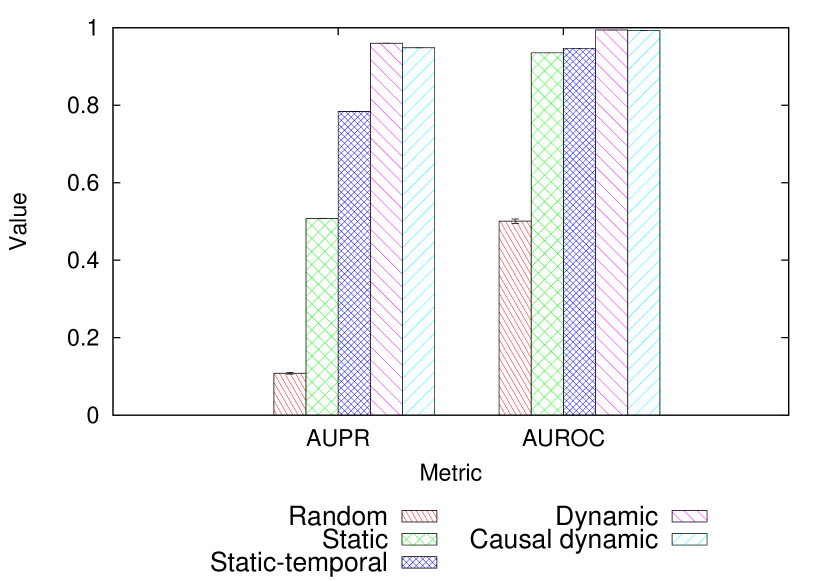
Figure 6: Network classification accuracy of the different methods in terms of AUPR and AUROC. For each method, the highest-scoring graphlet size is chosen. For other parameter choices, see Table I.

Figure 7: Network classification accuracy of the different methods in terms of precision-recall curves. For each method, the highest-scoring graphlet size is chosen. For other parameter choices, see Table I.

III-B Node classification

Also, we test how well the different methods distinguish between six different classes of nodes in a real-world network based on the nodes’ graphlet counts. The different evaluation criteria give consistent results: while according to Wilcoxon rank-sum test, all methods have intra-class distances significantly lower than inter-class distances and thus show non-random behavior ($p$-values less than $10^{-100}$), just as with network classification, (causal) dynamic graphlets are again superior both in terms of accuracy and computational complexity, followed by static-temporal graphlets, followed by static graphlets (Figure 8, Figure 9, and Table II).

Method	AUPR	AUROC	Break-even point	Maximum F-score	Running time, s
Static, 3-node	0.464	0.600	0.456	0.562	9.4
Static, 4-node	0.469	0.610	0.461	0.567	9.4
Static, 5-node	0.464	0.604	0.462	0.566	9.4
Static-temporal, 3-node	0.499	0.644	0.508	0.571	2.7
Static-temporal, 4-node	0.503	0.643	0.609	0.689	2.7
Static-temporal, 5-node	0.482	0.570	0.486	0.554	2.7
Dynamic, 3-event, 3-node	0.479	0.622	0.477	0.569	2.7
Dynamic, 5-event, 3-node	0.474	0.615	0.458	0.569	9.6
Dynamic, 7-event, 3-node	0.470	0.609	0.460	0.572	27.5
Dynamic, 3-event, 4-node	0.541	0.684	0.547	0.594	24.5
Dynamic, 6-event, 4-node	0.525	0.666	0.516	0.583	1,024
Dynamic, 4-event, 5-node	0.591	0.726	0.615	0.620	753
Causal dynamic, 3-event, 3-node	0.491	0.639	0.498	0.569	1.1
Causal dynamic, 5-event, 3-node	0.492	0.638	0.495	0.570	1.9
Causal dynamic, 7-event, 3-node	0.492	0.638	0.495	0.571	2.6
Causal dynamic, 3-event, 4-node	0.550	0.695	0.570	0.600	4.9
Causal dynamic, 6-event, 4-node	0.550	0.695	0.571	0.600	37.2
Causal dynamic, 4-event, 5-node	0.594	0.732	0.618	0.637	60.8
Causal dynamic, 5-event, 6-node	0.611	0.743	0.636	0.654	815
Causal dynamic, 6-event, 7-node	0.608	0.742	0.635	0.652	10,029
Random	0.376 (0.009)	0.495 (0.016)	0.369 (0.007)	0.550 (0.000)	-

TABLE II: Detailed node classification results for the different methods and different parameters in each method. The table can be interpreted just as Table I. Causal dynamic graphlet methods below the dashed line correspond to parameter choices that were not feasible to test with regular dynamic graphlets. Also, notice that in this test of node classification we could test some additional parameters (e.g., graphlets on five or more nodes) compared to the test of network classification (Table I); this is because the test of network classification is computationally much more complex, given that graphlets need to be counted in multiple networks, as opposed to counting graphlets in only one network in the node classification task.

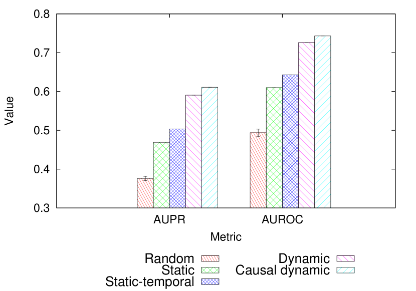
Figure 8: Node classification accuracy of the different methods in terms of AUPR and AUROC. For each method, the highest-scoring graphlet size is chosen. For other parameter choices, see Table II.

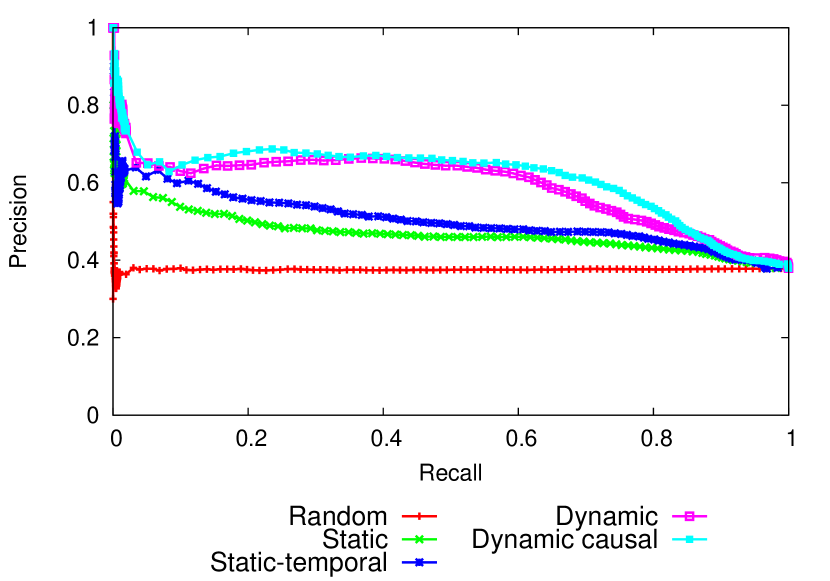
Figure 9: Node classification accuracy of the different methods in terms of precision-recall curves. For each method, the highest-scoring graphlet size is chosen. For other parameter choices, see Table II.

In this evaluation test of node classification, unlike in the test of network classification, the best parameter version of causal dynamic graphlets is more accurate than the best parameter version of dynamic graphlets. We note, however, that due to the differences in the counting process, causal dynamic graphlet counting allows us to consider larger graphlet sizes (e.g., six or seven nodes) that are not attainable when using regular dynamic graphlet counting due to computational constraints (Table II). And it is at these large graphlet sizes of six or seven nodes where causal dynamic graphlets peform the best. So, in order to evaluate which one is more accurate, dynamic graphlets or causal dynamic graphlets, it might not be fair to compare the two methods’ best parameter versions, due to differences in the considered graphlet sizes. Nonetheless, even if we compare dynamic and causal dynamic graphlets of the same size, we find that causal dynamic graphlets still demonstrate better results (Table II).

Further, in this evaluation test of node classification, unlike in the test of network classification, causal dynamic graphlet counting takes significantly less time than regular dynamic graphlet counting (Table II), which justifies our motivation behind causal dynamic graphlets.

Importantly, not only the different methods differ quantitatively, but they also lead to different qualitative results (Figure 10): there is a clear separation between static, static-temporal, and (causal) dynamic graphlets in terms of which nodes they describe as topologically similar. If we zoom into these results even further, within both dynamic and causal dynamic graphlets, we can see two clear clusters corresponding to three-node graphlets with different numbers of events. Thus, the number of nodes seems to play a larger role in separating the different dynamic graphlet methods compared to the number of events. (We discuss the effect of the method parameters in more detail in the following section.)

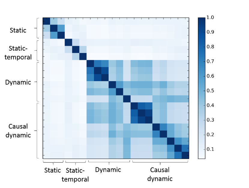
Figure 10: Pairwise similarities between the different methods and their parameter variations in the test of node classification. Similarities are computed as Jaccard similarity coefficients between two methods’ top 5% node pairs that are the closest in the graphlet-based PCA space. The order of the methods in the figure directly corresponds to the method order in Table II (we leave out detailed method names for visual clarity).

III-C Effect of graphlet size on results

Number of graphlet nodes. We next test the effect of graphlet size in terms of the number of nodes on the result quality (i.e., accuracy), for all four graphlet methods. For network classification, we surprisingly find that increasing the number of graphlet nodes leads to inferior accuracy, for all three graphlet-based methods (Table I). On the other hand, in node classification, for static and static-temporal graphlets, results are almost the same for all graphlet sizes, with 4-node graphlets showing marginally better performance, while for dynamic and causal dynamic graphlets, larger number of nodes leads to better accuracy (Table II). In terms of the running time (rather than accuracy), as expected, larger number of nodes leads to increase in computational complexity, independent on evaluation test or graphlet method.

Number of graphlet events. Also, we test the effect of graphlet size in terms of the number of events on the result quality (i.e., accuracy), for dynamic and causal dynamic graphlets (the other two graphlet methods, static and static-temporal graphlets, do not deal with the notion of events, i.e., temporal edges). For network classification, we surprisingly find that the number of events does not affect the accuracy (Table I). On other hand, in node classification, for a fixed number of nodes, the increase in the number of events leads to slight improvement in accuracy for dynamic graphlets but slight decrease in accuracy for causal dynamic graphlets (Table II). In terms of the running time (rather than accuracy), larger number of events leads to increase in computational complexity, although the level of running time increase is less pronounced than when increasing the number of nodes.

IV Conclusions

The increasing availability of temporal real-world network data has raised new challenges to the network researchers. While one can use the existing static approaches to study the aggregate or snapshot-based network representation of the temporal data, doing so overlooks important temporal information from the data. Hence, we develop a novel approach of dynamic graphlets that can capture the temporal information explicitly. In a systematic and thorough evaluation, we demonstrate the superiority of our approach over its static counterparts. This confirms that efficiently accounting for temporal information helps with structural and functional interpretation of the network data. This in turn illustrates real-life relevance of our new dynamic graphlet methodology, especially because the amount of available temporal network data is expected to continue to grow across many domains.

References

- [1] M. Newman, Networks: an introduction. Oxford University Press, 2010.
- [2] P. Holme and J. Saramäki, “Temporal networks,” Physics Reports, vol. 519, no. 3, pp. 97–125, 2012.
- [3] C. E. Priebe, J. M. Conroy, D. J. Marchette, and Y. Park, “Scan statistics on Enron Graphs,” Computational & Mathematical Organization Theory, vol. 11, no. 3, pp. 229–247, 2005.
- [4] J. Leskovec, L. Backstrom, R. Kumar, and A. Tomkins, “Microscopic evolution of social networks,” in Proceedings of the 14th ACM SIGKDD international conference on Knowledge discovery and data mining. ACM, 2008, pp. 462–470.
- [5] J. Leskovec, J. Kleinberg, and C. Faloutsos, “Graphs over time: densification laws, shrinking diameters and possible explanations,” in Proceedings of the eleventh ACM SIGKDD international conference on Knowledge discovery in data mining. ACM, 2005, pp. 177–187.
- [6] T. M. Przytycka, M. Singh, and D. K. Slonim, “Toward the dynamic interactome: it’s about time,” Briefings in bioinformatics, p. bbp057, 2010.
- [7] M. Valencia, J. Martinerie, S. Dupont, and M. Chavez, “Dynamic small-world behavior in functional brain networks unveiled by an event-related networks approach,” Physical Review E, vol. 77, no. 5, p. 050905, 2008.
- [8] Milenković, Tijana and Lai, Jason and Pržulj, Nataša, “GraphCrunch: a tool for large network analyses,” BMC Bioinformatics, vol. 9, no. 1, p. 70, 2008.
- [9] R. Milo, S. Shen-Orr, S. Itzkovitz, N. Kashtan, D. Chklovskii, and U. Alon, “Network motifs: simple building blocks of complex networks,” Science, vol. 298, no. 5594, pp. 824–827, 2002.
- [10] R. Milo, S. Itzkovitz, N. Kashtan, R. Levitt, S. Shen-Orr, I. Ayzenshtat, M. Sheffer, and U. Alon, “Superfamilies of evolved and designed networks,” Science, vol. 303, no. 5663, pp. 1538–1542, 2004.
- [11] Y. Artzy-Randrup, S. J. Fleishman, N. Ben-Tal, and L. Stone, “Comment on ”network motifs: simple building blocks of complex networks” and ”superfamilies of evolved and designed networks”,” Science, vol. 305, no. 5687, pp. 1107–1107, 2004.
- [12] T. Milenković, I. Filippis, M. Lappe, and N. Pržulj, “Optimized null model for protein structure networks,” PLOS ONE, vol. 4, no. 6, p. e5967, 2009.
- [13] N. Pržulj, D. G. Corneil, and I. Jurisica, “Modeling interactome: scale-free or geometric?” Bioinformatics, vol. 20, no. 18, pp. 3508–3515, 2004.
- [14] T. Milenković and N. Pržulj, “Uncovering biological network function via graphlet degree signatures.” Cancer Informatics, no. 6, 2008.
- [15] T. Milenković, W. L. Ng, W. Hayes, and N. Pržulj, “Optimal network alignment with graphlet degree vectors,” Cancer Informatics, vol. 9, p. 121, 2010.
- [16] O. Kuchaiev, T. Milenković, V. Memišević, W. Hayes, and N. Pržulj, “Topological network alignment uncovers biological function and phylogeny,” Journal of the Royal Society Interface, vol. 7, pp. 1341–1354, 2010.
- [17] V. Saraph and T. Milenković, “MAGNA: Maximizing Accuracy in Global Network Alignment,” Bioinformatics, vol. 30, no. 20, pp. 2931–2940, 2014.
- [18] R. W. Solava, R. P. Michaels, and T. Milenković, “Graphlet-based edge clustering reveals pathogen-interacting proteins,” Bioinformatics, vol. 28, no. 18, pp. i480–i486, 2012.
- [19] Y. Hulovatyy, S. D’Mello, R. A. Calvo, and T. Milenković, “Network analysis improves interpretation of affective physiological data,” Journal of Complex Networks, 2014.
- [20] Y. Hulovatyy, R. W. Solava, and T. Milenković, “Revealing missing parts of the interactome via link prediction,” PLOS ONE, vol. 9, no. 3, p. e90073, 2014.
- [21] F. E. Faisal and T. Milenković, “Dynamic networks reveal key players in aging,” Bioinformatics, p. btu089, 2014.
- [22] F. Faisal, H. Zhao, and T. Milenković, “Global Network Alignment In The Context Of Aging,” Computational Biology and Bioinformatics, IEEE/ACM Transactions on Computational Biology and Bioinformatics, vol. PP, no. 99, 2014.
- [23] T. Milenković, V. Memišević, A. K. Ganesan, and N. Pržulj, “Systems-level cancer gene identification from protein interaction network topology applied to melanogenesis-related functional genomics data,” Journal of The Royal Society Interface, vol. 7, no. 44, pp. 423–437, 2010.
- [24] H. Ho, T. Milenković, V. Memišević, J. Aruri, N. Pržulj, and A. Ganesan, “Protein interaction network uncovers melanogenesis regulatory network components within functional genomics datasets,” BMC Systems Biology, vol. 4, no. 84, 2010.
- [25] T. Milenković, V. Memišević, A. Bonato, and N. Pržulj, “Dominating biological networks,” PLOS ONE, vol. 6, no. 8, p. e23016, 2011.
- [26] V. Nicosia, J. Tang, M. Musolesi, G. Russo, C. Mascolo, and V. Latora, “Components in time-varying graphs,” Chaos: An Interdisciplinary Journal of Nonlinear Science, vol. 22, no. 2, p. 023101, 2012.
- [27] D. Braha and Y. Bar-Yam, “Time-dependent complex networks: Dynamic centrality, dynamic motifs, and cycles of social interactions,” in Adaptive Networks. Springer, 2009, pp. 39–50.
- [28] Q. Zhao, Y. Tian, Q. He, N. Oliver, R. Jin, and W.-C. Lee, “Communication motifs: a tool to characterize social communications,” in Proceedings of the 19th ACM international conference on Information and knowledge management. ACM, 2010, pp. 1645–1648.
- [29] P. Bajardi, A. Barrat, F. Natale, L. Savini, and V. Colizza, “Dynamical patterns of cattle trade movements,” PLOS ONE, vol. 6, no. 5, p. e19869, 2011.
- [30] L. Kovanen, M. Karsai, K. Kaski, J. Kertész, and J. Saramäki, “Temporal motifs in time-dependent networks,” Journal of Statistical Mechanics: Theory and Experiment, vol. 2011, no. 11, p. P11005, 2011.
- [31] L. Kovanen, K. Kaski, J. Kertész, and J. Saramäki, “Temporal motifs reveal homophily, gender-specific patterns, and group talk in call sequences,” Proceedings of the National Academy of Sciences, vol. 110, no. 45, pp. 18 070–18 075, 2013.
- [32] D. Jurgens and T.-C. Lu, “Temporal motifs reveal the dynamics of editor interactions in wikipedia.” in ICWSM, 2012.
- [33] T. Hočevar and J. Demšar, “A combinatorial approach to graphlet counting,” Bioinformatics, vol. 30, no. 4, pp. 559–565, 2014.
- [34] D. Marcus and Y. Shavitt, “Rage–a rapid graphlet enumerator for large networks,” Computer Networks, vol. 56, no. 2, pp. 810–819, 2012.
- [35] Ö. N. Yaveroğlu, N. Malod-Dognin, D. Davis, Z. Levnajic, V. Janjic, R. Karapandza, A. Stojmirovic, and N. Pržulj, “Revealing the hidden language of complex networks,” Scientific Reports, vol. 4, 2014.
- [36] A.-L. Barabási and R. Albert, “Emergence of scaling in random networks,” Science, vol. 286, no. 5439, pp. 509–512, 1999.
- [37] J. Davis and M. Goadrich, “The relationship between precision-recall and roc curves,” in Proceedings of the 23rd international conference on Machine learning. ACM, 2006, pp. 233–240.
- [38] O. Kuchaiev, A. Stevanović, W. Hayes, and N. Pržulj, “GraphCrunch 2: software tool for network modeling, alignment and clustering,” BMC Bioinformatics, vol. 12, no. 1, p. 24, 2011.