Abstract

We study matter with central charge $c>1$ coupled to two-dimensional (2d) quantum gravity, here represented as causal dynamical triangulations (CDT). 2d CDT is known to provide a regularization of (Euclidean) 2d Hořava-Lifshitz quantum gravity. The matter fields are massive Gaussian fields, where the mass is used to monitor the central charge $c$. Decreasing the mass we observe a higher order phase transition between an effective $c=0$ theory and a theory where $c>1$. In this sense the situation is somewhat similar to that observed for “standard” dynamical triangulations (DT) which provide a regularization of 2d quantum Liouville gravity. However, the geometric phase observed for $c>1$ in CDT is very different from the corresponding phase observed for DT.

email: ambjorn@nbi.dk
email: goerlich@nbi.dk, atg@th.if.uj.edu.pl
email: jerzy.jurkiewicz@uj.edu.pl
email: zhang@th.if.uj.edu.pl

1 Introduction

Two-dimensional models of quantum gravity are useful toy models when it comes to study a number of conceptual problems related to a theory of quantum gravity: how do we define diffeomorphism invariant observables, how do we define distance when we at the same time integrate over geometries etc…? Some two-dimensional models have the further advantage that they can be solved analytically both as continuum quantum field theories and as regularized “lattice” theories. Quantum Liouville gravity (2d Euclidean quantum gravity) can be solved as a conformal field theory [1, 2, 3] and also using dynamical triangulations (DT) [4, 5, 6]. Similarly 2d (Euclidean) quantum Hořava-Lifshitz gravity (HLG) [7] can be solved both using continuum methods and as a lattice theory [8]. In both cases there seems to be a $c=1$ barrier: the geometries for $c<1$ and $c>1$ look completely different. However, it has not been easy to study the transition in either of the cases since no analytic solutions exist for $c>1$ and since it is difficult to vary $c$ continuously in numerical simulations.

The exist many numerical studies (and a few analytic studies) of DT coupled to matter in the $c>1$ region (for a partial list see [9]), and a few numerical studies of CDT coupled to matter in the same region [10, 11]. In this paper we will study the transition from $c<1$ to $c>1$ in a CDT model coupled to four Gaussian matter fields. In order to be able to interpolate between the two regimes we introduce a mass for the Gaussian fields. When the mass is large (of the order of the inverse lattice spacing) we expect the Gaussian fields to decouple from the geometry The geometry will then be that of pure 2d HLG. If the mass is zero the Gaussian fields will represent a conformal field theory with $c=4$. We have already studied this system numerically [11] and we observed a change of the geometry compared to the $c=0$ case. Decreasing the mass will bring us from $c=0$ to $c=4$. On the way we will observe a phase transition between to the two geometric regimes.

Let us briefly describe what has already been observed before the present study. The numerical studies of 1+1 dimensional CDT are conducted using an (Euclidean) spacetime with topology $S^{1}\times S^{1}$. The choice of a periodic (imaginary) time direction is mainly for numerical convenience and will not play a role as an indicator of finite temperature (the time extent can always be considered long, relative to any finite temperature considerations). In the original formulation of the CDT model in 1+1 dimensions [12] the geometry is represented by a discretized spacetime built of triangles. The vertices of triangles are located at integer times, with two vertices at a time $t$ and one at $t\pm 1$. Spatial slices at the discrete integer-labeled times then have the topology of a circle $S^{1}$. Equivalently, one can use the dual lattice with points in the centers of triangles connected by links, dual to the links of the triangles. The dual vertices are placed at half-integer times. In the dual formulation each vertex is connected to three other vertices, two of which are neighbors in the same time slice and one which lies in the half-integer time slice positioned above or below. Links joining vertices with the same time index form (together with the corresponding vertices) “space” at that given time, and spatial topology is $S^{1}$. In this paper we use this dual formulation.

Without matter fields the model can be solved analytically [12]. Let $\langle n(t)\rangle$ denote the average spatial volume measured at (half-integer) time $t$. If the time direction has length $L$ and the spacetime volume is $N$ we have $\langle n(t)\rangle=N/L$. The fluctuations around this average value can also be calculated analytically. If we couple matter fields to the geometry, one observes the same (trivial) picture as long as the central charge $c\leq 1$ for the matter fields [13]. However, if $c>1$ one observes a change in the behavior of the universe [10, 11]. If one looks at the distribution $n(t)$ in a single 1+1 dimensional universe generated by Monte Carlo simulations one observes a “blob” and a “stalk”. In the stalk $n(t)$ is of the order of the cut-off. In the computer simulations we do not allow $n(t)$ to shrink to zero which would result in disconnected universes and we thus put in a lower cut off $n(t)=2$. In the blob we have large $n(t)$’s and the average time extent of the blob scales as $N^{1/3}$, independent of $L$ if $L$ is larger than the size of the blob. As a function of computer time the “center of volume” of the blob is performing a random walk in the periodic time direction and to measure average properties of the blob we have to break the translation symmetry in our periodic discrete time. For each configuration we define $t=0$ as the “center of volume” of the blob In this way one can obtain the average spatial volume distribution of the blob with high accuracy:

$$\langle n(t)\rangle=\frac{2}{\pi}\alpha\,N^{1-1/3}\cos^{2}\left(\alpha\frac{t}{N^{1/3}}\right),~{}~{}~{}~{}|t|<\frac{\pi N^{1/3}}{2\alpha}.$$ (1)

with $\alpha$ being a constant which depends on the central charge $c>1$ of the matter fields, typically growing with $c$ [11]. The formula is only valid for the blob, i.e. in the $t$ range indicated in eq. (1). For $t$ outside this range we are in the stalk and $n(t)$ is of the order of the cut off. For large spacetime volume $N$ the effect of the stalk can be neglected when discussing properties of the blob. The scaling of the blob as a function of the size $N$ is precisely what one expects for (a deformed) sphere $S^{3}$, $t$ being the distance from equator and we thus say that the Hausdorff dimension of the average two-dimension graph representing the blob is $D_{H}=3$.

2 The model

A massless Gaussian field has central charge $c=1$. Thus $d$ Gaussian fields have central charge $d$. In this paper we couple $d$ Gaussian fields to the geometry using the CDT model. The scalar fields $\phi_{i}^{\mu},~{}\mu=1,\dots d$ are located at the vertices of the dual lattice. The combined system of geometry and matter is then a statistical model described by the partition function

$$Z=\sum_{T}\frac{1}{S_{T}}\;\mbox{e}^{-\lambda N_{T}}\int\prod_{i,\mu}d\phi_{i}^{\mu}\mbox{e}^{-S_{measure}(\phi_{i}^{\mu},m)}$$ (2)

where $\lambda$ is a cosmological constant, $N_{T}$ is the number of vertices in the graph dual to the triangulation $T$ and $S_{T}$ is a symmetry factor of the graph (the order of the automorphism group of the graph). The Gaussian measure (or action) $S_{measure}$ is defined as

$$S_{measure}(\phi_{i}^{\mu},m)=\frac{1}{2}\sum_{l_{ij},\mu}(\phi_{i}^{\mu}-\phi_{j}^{\mu})^{2}+m^{2}\sum_{i,\mu}\left(\phi_{i}^{\mu}\right)^{2},$$ (3)

where $l_{ij}$ is the link between vertices $i$ and $j$ and where we have also added a mass term to the action.

It is convenient to use $d$ massless Gaussian fields in the simulations if we want to study the effect of matter with central charge $d$ on the geometry. In contrast, using $2d$ Ising spins would require that we first locate the critical point of these Ising spins coupled to the geometry and then conduct the simulations precisely at this critical point. Massless Gaussian fields are automatically critical. Using such massless Gaussian fields we have measured the scaling (1) for various $d>1$.

However, it is difficult to study in detail the change of geometry between the regime with $c<1$ and $c>1$ using massless Gaussian fields since $d$ is an integer. In order to induce a continuous change between the two regimes we thus introduce a mass term for the Gaussian fields. We start out with $d=4$ massless fields and by increasing the mass we will eventually for large mass have a system which effectively has $c=0$. In principle one could obtain the same effect for multiple Ising spins by moving gradually away from the critical point, but the procedure is much more difficult to control numerically.

The role of the mass parameter in the action $S_{measure}$ can be can be made clear by redefining the field variables by $\psi_{i}^{\mu}=m\phi_{i}^{\mu}$. Thus the action becomes

$$S_{measure}(\psi_{i}^{\mu},m)=\frac{1}{2m^{2}}\sum_{l_{ij},\mu}(\psi_{i}^{\mu}-\psi_{j}^{\mu})^{2}+\sum_{i,\mu}\left(\psi_{i}^{\mu}\right)^{2}$$ (4)

and the the integration measure simply redefines the cosmological constant

$$\prod_{i,\mu}d\phi_{i}^{\mu}=m^{-dN_{T}}\prod_{i,\mu}d\psi_{i}^{\mu}$$ (5)

For large $m$ we can neglect the couplings between the neighboring vertices in $S_{measure}(\psi,m)$ and as a consequence, up to a redefinition of the cosmological constant, we can eliminate the fields completely and obtain the pure gravity system. For large $m$ we thus expect a behavior qualitatively identical to pure gravity for all geometric observables. In the small $m$ limit we expect to observe the same kind of geometries as observed for massless Gaussian fields.

Typical configurations for various choices of masses are shown in Fig. 1 when we have four Gaussian fields. We see a blob for small masses, it gets broader with increasing mass and it finally disappears for large masses. This will be seen even better when we study the average profile of the blob.

Figure 1: Individual configurations $n(t,m^{2})$ for $d=4$, $m^{2}=0.00$ (top left), 0.05 (top right), 0.15 (bottom left) and 0.20 (bottom right). In all cases we center the distribution so that the center of volume is shifted to $t=0$.

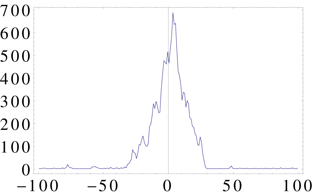
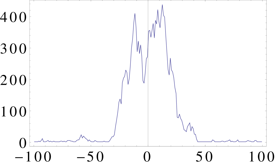
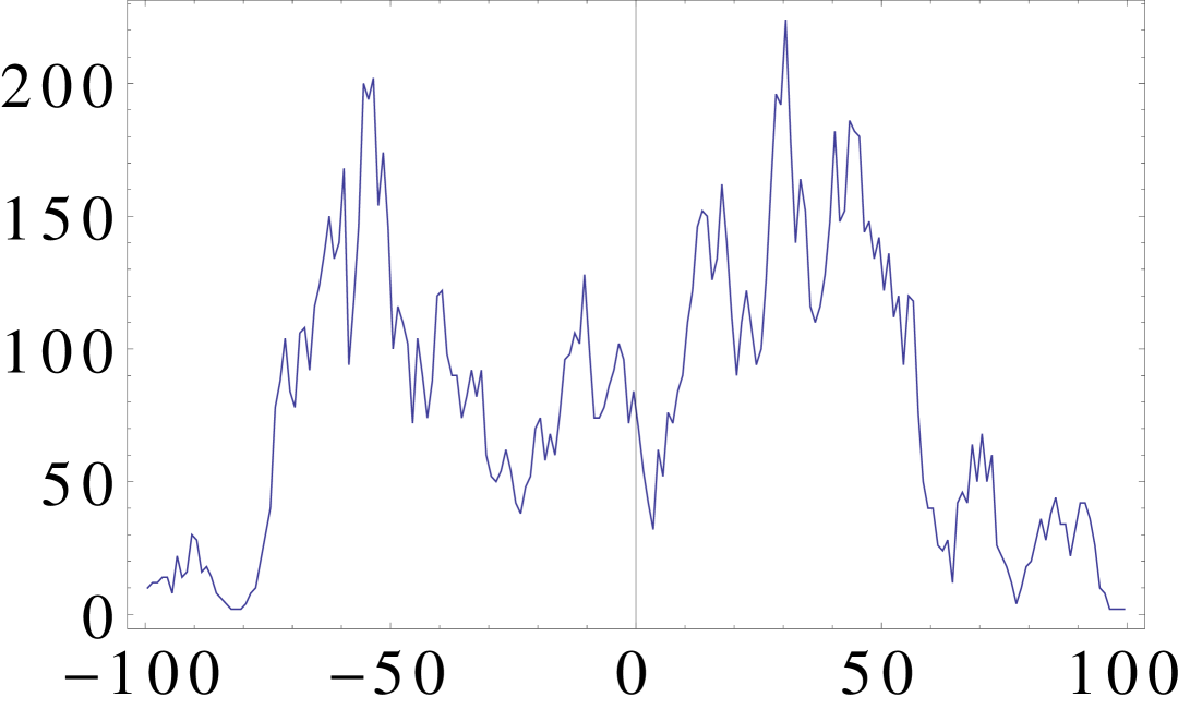
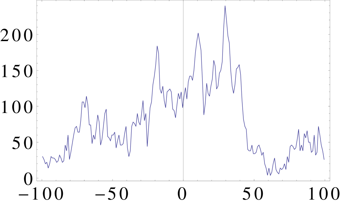
In the next Sections we shall quantify these effects and try to determine a transition between the two regimes as a function of the mass parameter $m^{2}$.

3 Mass dependence of the volume profiles

3.1 Small masses

For a small mass $m^{2}$ the average profile of spatial volumes $\langle n(t,m^{2})\rangle$ contains a central blob where $\langle n(t,m^{2})\rangle\gg 2$ and a stalk where $\langle n(t,m^{2})\rangle$ is of the cut-off size 2. In Fig. 2 we show the dependence of the volume profiles for a fixed total volume $N=16000$ and a sequence of time periods $L$. We see that the thickness (the spatial volume $\langle n(t,m^{2})\rangle$) of the stalk does not change with $L$. The peaks of the blobs get slightly reduced for larger $L$ since more and more volume is shifted to the stalk with increasing $L$.

Figure 2: Average spatial volume distribution $\langle n(t,m^{2})\rangle$ for a fixed spacetime volume $N=16000$ and $m^{2}=0.01$ (top) and 0.05 (bottom) and time periods $L=200,~{}400,~{}600$. On the left plots we show the whole range of times $-L/2<t<L/2$. On the right plots we zoom in on the onset of the stalk regime in order to show that the stalk is independent of $L$.

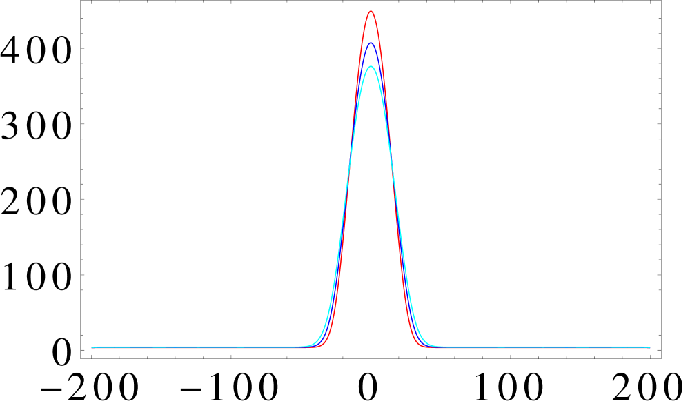
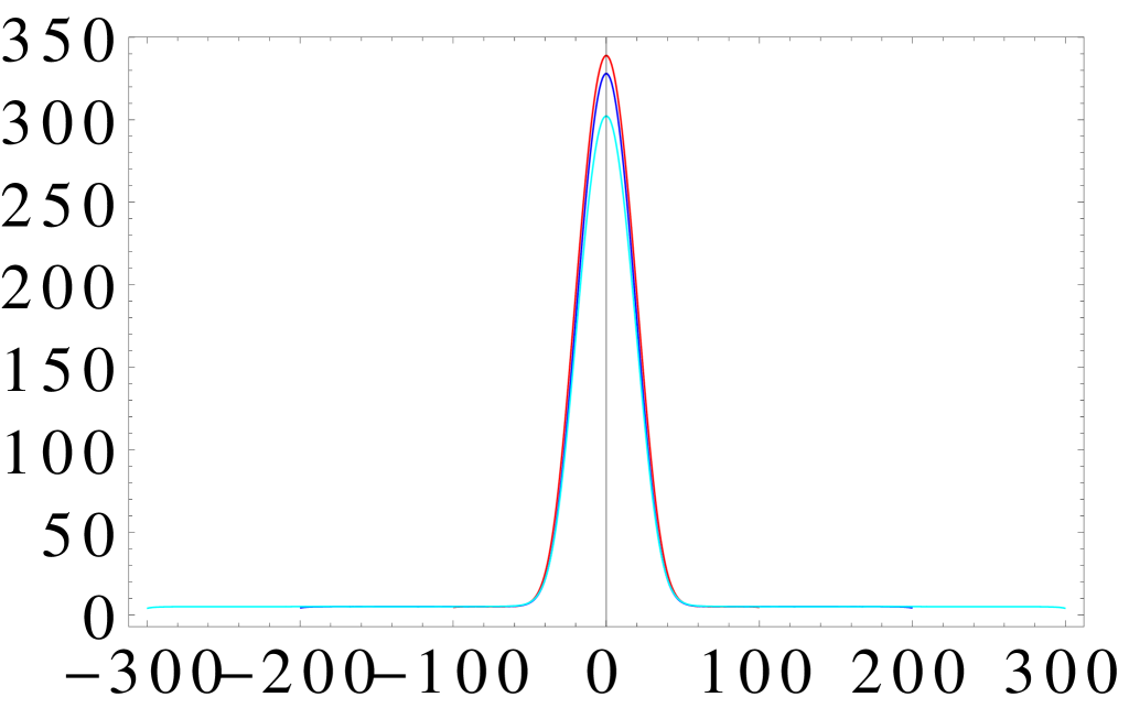
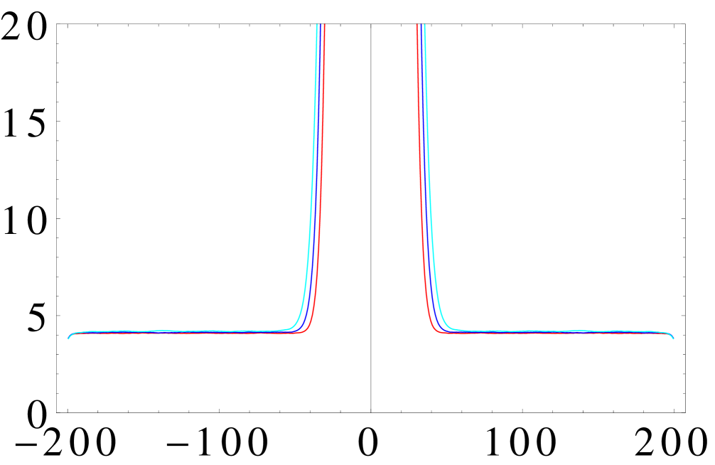
In addition the thickness of the stalk does not change with the total volume $N$ (provided of course that $L$ is big enough to contain both the blob and a stalk). $\langle n(t,m^{2})\rangle$ in the stalk depends on the mass and grows with $m^{2}$. The values are given in the Table.1 for $0\leq m^{2}\leq 0.07$. For this range of masses they are still of the order of the cut off.

$m^{2}$	0.00	0.01	0.02	0.03	0.04	0.05	0.06	0.07
$h$	3.75	3.82	3.96	4.22	4.48	4.84	5.43	6.29

Table 1: Average spatial volume $\langle n(t,m^{2})\rangle$ in the stalk for $0.00<m^{2}<0.07$

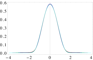
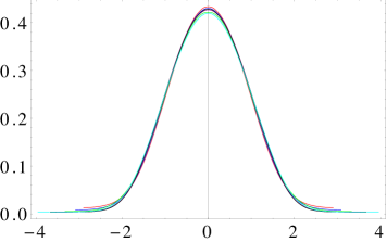
For $t$ in the blob range, $\langle n(t,m^{2})\rangle$ scales with $N$ in a way consistent with a Hausdorff dimension $D_{H}=3$, i.e. the time extent of the blob scales as $N^{1/3}$. In Fig. 3 we illustrate the scaling to a distribution $\rho(\tau,m^{2})=N^{1/D_{H}-1}n(t,m^{2})$, independent of $N$, plotted as a function of the scaled time variable $\tau=t/N^{1/D_{H}}$. The requirement of a scaling function $\rho(\tau,m^{2})$ for different spacetime volumes $N$ determines $D_{H}=3$ with good precision for all small values of $m^{2}$.

Figure 3: The scaling function $\rho(\tau,m^{2})$ which scales in the the blob range (but not in the stalk region), shown for two masses $m^{2}=0.01$ (left) and 0.05 (right) for a sequence of spacetime volumes $N$. Notice the change of scale for the different masses. The combination of volumes and lengths are: ($N=10000,~{}L=100$), ($N=14400,~{}L=120$), ($N=22500,~{}L=150$), ($N=32400,~{}L=180$), ($N=40000,~{}L=200$), ($N=62500,~{}L=250$).

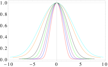
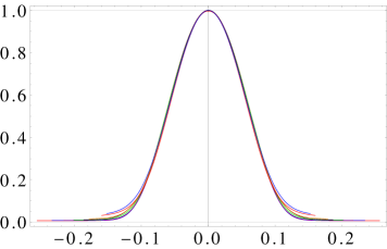
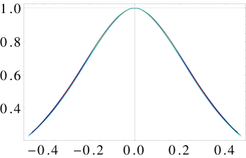
However, the universality is even larger. For small masses all distributions $\langle n(t,m^{2})\rangle$ can be made to coincide if we, rather than scaling the time as $\tau=t/N^{1/3}$, define a rescaled time which depends on the mass: $\tilde{\tau}=\alpha(m^{2})\tau$ and redefine the height of distribution accordingly as $\tilde{\rho}(\tilde{\tau})=(\alpha(m^{2}))^{-1}N^{1/3-1}n(t,m^{2})$. A comparison of the rescaled distributions $\tilde{\rho}(\tilde{\tau})$ for $m^{2}\in[0.01,0.09]$ is presented on Fig. 4. The left curves are obtained by keeping the time variable $\tau$ unchanged but rescaling the maximum height of the curves to the $m^{2}=0$ curve (which is equivalent to multiplying $\rho(\tau,m^{2})$ with $\alpha(0)/\alpha(m^{2})$, provided a universal $\tilde{\rho}(\tilde{\tau})$ exists). The right curves are then obtained by rescaling $\tau$ to $\tilde{\tau}$ for the various curves, and in this way determining $\alpha(m^{2})/\alpha(m^{2}=0)$ as the value leading to maximal overlap with the $m^{2}=0$ curve. It thus follows from (1) that

$$\tilde{\rho}(\tilde{\tau})=\frac{2}{\pi}\cos^{2}{\tilde{\tau}},~{}~{}~{}~{}\tau\in[-\pi/2,\pi/2].$$ (6)

The $\alpha$ values drop for larger mass (see Fig. 8 for the plot of $\alpha(m^{2})/\alpha(0)$), implying that the blob gets broader when expressed in the unscaled time-variable. However, using the rescaled variable $\tilde{\tau}$ we can talk about one universal scaling distribution (6) of spatial volumes in the “blob” phase, independent of the mass for $m^{2}\in[0,0.09]$.

Figure 4: Scaling for small masses $m^{2}\in[0,0.09]$: the left plot shows the distributions $\frac{\rho(\tau,m^{2})}{\alpha(m^{2})}\frac{\alpha(0)}{\rho(\tau,0)}$ plotted as functions of $\tau=t/N^{1/3}$. The right plot shows the same ratio plotted as a function of $\tilde{\tau}=\alpha(m^{2})\tau$, where the factors $\alpha(m^{2})$ are determined by maximizing the overlap between the various curves. The universal curve that emerges on the right plot is $\tilde{\rho}(\tilde{\tau})$ up to a normalization factor $\pi/2$ (see eq. (6)).

3.2 Large masses

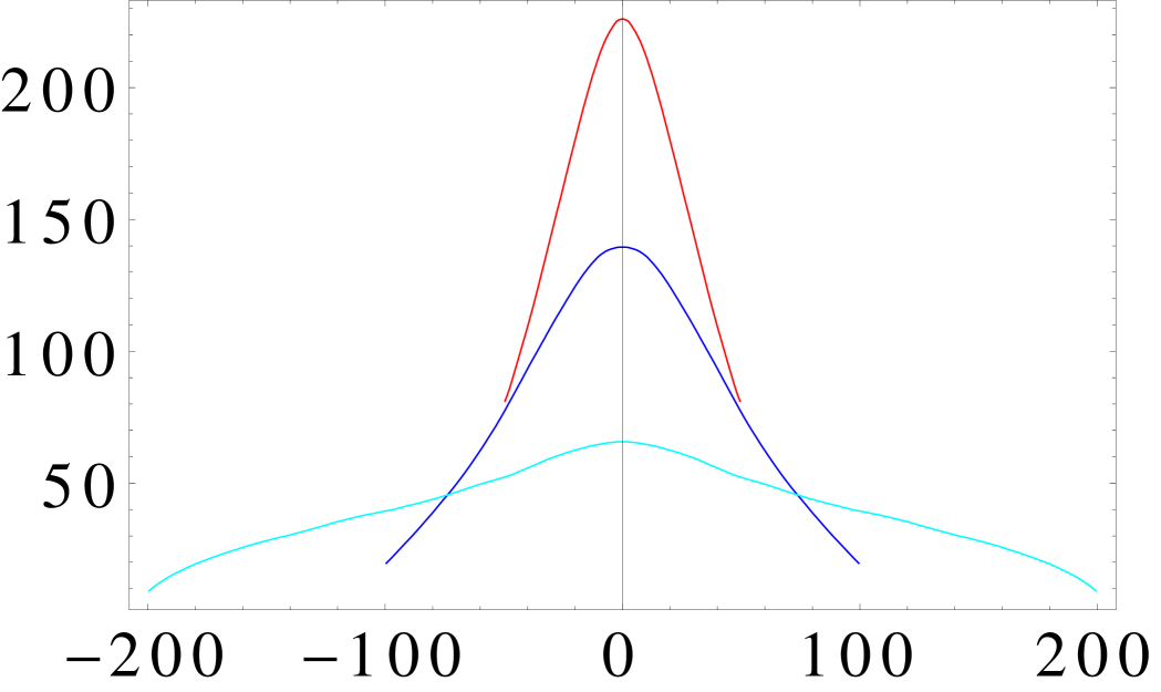
The behavior is different for masses $m^{2}\geq 0.15$. As was explained above we expect for large masses that $\langle n(t,m^{2})\rangle$ will be qualitatively similar to the pure gravity case, where it is known analytically that any scaling should correspond to a Hausdorff dimension $D_{H}=2$. In our approach we use the same method to center the volume of individual configurations as we used in the case where we observed a genuine blob (see footnote 2). As a consequence we see an artificial maximum around time $t=0$, as already mentioned in footnote 3. The stalk is absent, and the distributions have triangular shapes, with the height depending on the assumed period $L$ as $1/L$. Thus

$$\langle n(t,m^{2})\rangle=\frac{N}{L}f(t/L,m^{2}),~{}~{}~{}\int_{-1/2}^{1/2}f(x,m^{2})dx\approx 1.$$ (7)

This is illustrated in Fig. 5.

Figure 5: $\langle n(t,m^{2})\rangle$ for $m^{2}=0.15$ (left) and 0.20 (right) for different $L$ and a fixed spacetime volume $N=16000$.

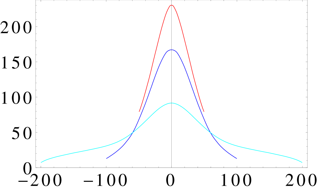
If we want to look for scaling behavior of $\langle n(t,m^{2})\rangle$ when changing $N$, we have to change the length of the time period $L$ simultaneously as $L\propto N^{1/2}$ since there is no stalk. For the choice $L=\sqrt{N}$ eq. (7) reads

$$\langle n(t,m^{2})\rangle=N^{1/2}f(t/N^{1/2},m^{2}).$$ (8)

For each value of $m^{2}\geq 0.15$ we can extract a scaling function $f(\tau,m^{2})$, $\tau=t/N^{1/2}$, by varying $N$, as illustrated in Fig. 6. When comparing (8) with the general scaling form $N^{1-1/D_{H}}f(t/N^{1/D_{H}},m^{2})$ we see that the observed scaling indeed is compatible with $D_{H}=2$.

Figure 6: The scaling function $f(\tau,m^{2})$, $\tau=t/L$ as it appears by collapsing the various graphs $N^{1/D_{H}-1}\langle n(t,m^{2})\rangle$ for $m^{2}=0.15$ (left) and 0.20 (right), with $D_{H}=2$. The combination of volumes and lengths are: ($N=10000,~{}L=100$), ($N=14400,~{}L=120$), ($N=22500,~{}L=150$), ($N=32400,~{}L=180$), ($N=40000,~{}L=200$),($N=62500,~{}L=250$).

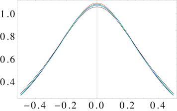
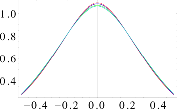
In the same way as we did for the small masses, we now try to find a universal scaling of $\langle n(t,m^{2})\rangle$ for all large masses. We construct the universal function in two steps, starting from the scaling functions $f(\tau,m^{2})$, $\tau=t/N^{1/2}$, we already have available for each $m^{2}$. First we scale these functions such that they agree at $\tau=0$ using $f(\tau,m_{max}^{2})$ as reference, i.e.

$$\hat{f}(\tau,m^{2})=\frac{f(0,m^{2}_{max})}{f(0,m^{2})}\,f(\tau,m^{2}),$$ (9)

The result is shown in the left plot in Fig. 7.

Figure 7: The function $\hat{f}(\tau,m^{2})$ (left plot) and the universal scaling function $\tilde{f}(\tilde{\tau})$ (right plot) for $m^{2}\in[0.12,0.18]$.

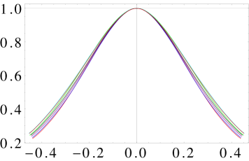
Then we try to rescale the time variable as we did for the small masses: $\tilde{\tau}=\beta(m^{2})\,t/L$, where the function $\beta(m^{2})$ is determined to ensure maximal overlap. This results in our universal scaling function

$$\tilde{f}(\tilde{\tau})=\hat{f}(\tau,m^{2}),~{}~{}~{}~{}\tilde{\tau}=\beta(m^{2})\tau$$ (10)

The result is shown in the right plot in Fig. 7 and the function $\beta(m^{2})$ is shown Fig. 8. Note that this procedure results in overlapping graphs, but not in the same range of the common scaling variable $\tilde{\tau}$. This is in contrast to the situation for small masses, the reason being that for small masses the original $t$ range was a “physical” range, namely the time extent of the blob, which was a function of $m^{2}$ and our rescaling $\tilde{\tau}=\alpha(m^{2})\tau$ made the time extent of the blobs agree and thus, if we had first adjusted the maximum height of the blobs, would also ensure the collapse of the blobs to a universal curve (assuming such one exists). In the large mass case we have no blob and by definition the range of $t$ is from $-L/2$ to $L/2$. Thus, by in addition choosing $L=N^{1/2}$ and $\tau=t/N^{1/2}$ we have also chosen the range of $\tau$ to be identical for the various large masses. Redefining $\tau$ to $\tilde{\tau}$ will then change the range of $\tilde{\tau}$ for the various masses and we can only talk about the overlap of functions in the common $\tilde{\tau}$ region. One could have compensated for this by choosing from the outset different $L$’s according to $L=L/\beta(m^{2})$ and one would have had a starting point similar to the small mass case where the range of $t$ was mass dependent. From this point of view it makes sense to talk about one universal scaling function associated with $\langle n(t,m^{2})\rangle$ also in the large mass regime, and this scaling function can be extracted from pure CDT without matter fields, which is the limit of $m^{2}\to\infty$. From Fig. 8 it is seen that the function $\beta(m^{2})$ is 1 for $m^{2}>0.18$. $m^{2}=\infty$ thus effectively starts at $m^{2}=0.18$.

Figure 8: Possible range of the phase transition: $\alpha(m^{2})/\alpha(0)$ is the scale factor for the small masses and $\beta(m^{2})/\beta(\infty)$ the scaling factor for large masses. The Hausdorff dimension is respectively $D_{H}=3$ and $D_{H}=2.0$ .

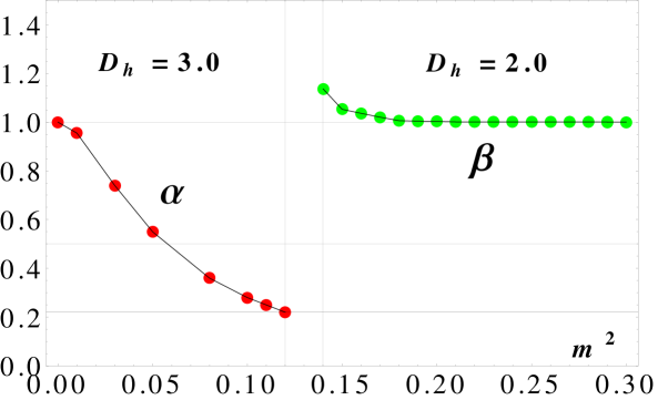
On the fig.8 we show values of $\alpha(m^{2})/\alpha(0)$ and $\beta(m^{2})/\beta(\infty)$ as functions of $m^{2}$. For $m^{2}\in[0.10,0.14]$ there is a cross over between the two well defined regimes corresponding to $D_{H}=3$ and $D_{H}=2$, respectively. In this range none of the fitting prescriptions described above work and using scaling arguments alone do not allow us to determine if there is a genuine phase transition or just a rapid cross over between the $D_{H}=3$ and the $D_{H}=2$ regions of $m^{2}$.

4 Study of the phase transition

In order to study better the change from $D_{H}=3$ to $D_{H}=2$ we introduce the so-called volume-volume correlator $\langle\mathrm{corr}(\Delta)\rangle$, where $\mathrm{corr}(\Delta)$ is defined for individual configurations as

$$\mathrm{corr}(\Delta)=\sum_{i=1}^{L}n(t_{i})n(t_{i}+\Delta)$$ (11)

A great advantage of using the correlation function (11) is that one does not need to identify and to center the blob and it is well defined even if there is no blob.

A correlator similar to that defined by (11) was used in numerical studies of the scaling in three and four-dimensional CDT [15]. We will measure $\mathrm{corr}(\Delta)$ at the maximal separation $\Delta=L/2$. In the small mass regime, where the blob is well localized we expect a behavior

$$\langle\mathrm{corr}(L/2)\rangle\approx 2hN$$ (12)

where $h$ is the average spatial volume of the time slices belonging to the stalk. As a consequence we expect in this mass regime that $\langle\mathrm{corr}(L/2)\rangle/N\approx 2h$, i.e.  approximately both $N$ and $L$ independent. In the large mass regime we expect a different behavior

$$\langle\mathrm{corr}(L/2)\rangle\approx N^{2}/L$$ (13)

and consequently $L\langle\mathrm{corr}(L/2)\rangle/N^{2}\approx 1$ should be $N$ and $L$ independent. In our analysis we fix the time period $L$ and the spacetime volume $N$ and measure the correlator as a function of $m^{2}$. In Fig. 9 we show the typical behavior of $\langle\mathrm{corr}(L/2)\rangle/N$ and $L\langle\mathrm{corr}(L/2)\rangle/N^{2}$ for $L=800$ and a sequence of spacetime volumes $N$. The plots illustrate the difference between the small and large mass behavior and indicate that there is a well defined transition between the two regimes.

Figure 9: The dependence of $\langle\mathrm{corr}(L/2)\rangle/N$ and $L\langle corr(L/2)\rangle/N^{2}$ on the mass in the range between $m^{2}=0.01$ and $m^{2}=0.30$ Both plots are for $L=800$ with spacetime volumes $N=$ 8000, 16000, 24000, 32000 and 40000.

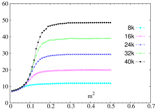
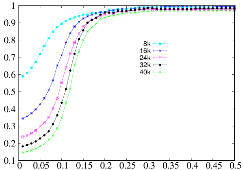
To substantiate this we calculate the derivative $\mbox{d}\langle\mathrm{corr}(L/2)\rangle/\mbox{d}m^{2}$. It has a clear peak growing with the size $N$ of the system and thus signals a phase transition transition. In Fig. 10 we show the values of the numerically estimated derivative $(1/N)\Delta\langle\mathrm{corr}(L/2)\rangle/\Delta m^{2}$ as a function of $m^{2}$ for $L=800$ and for a sequence of spacetime volumes $N$ (left plot) and the peak values of the estimated derivatives as a function of $N$ (right plot).

Figure 10: $(1/N)\Delta\langle\mathrm{corr}(L/2,m^{2})\rangle/\Delta m^{2}$ for $m^{2}\in[0.01,0.30]$ (left). The curves correspond to $N=$ 8000, 16000, 24000, 32000 and 40000 and $L=800$. The right figure shows the maximum as a function of $N$, the curve being a fit to $N^{1.5}$.

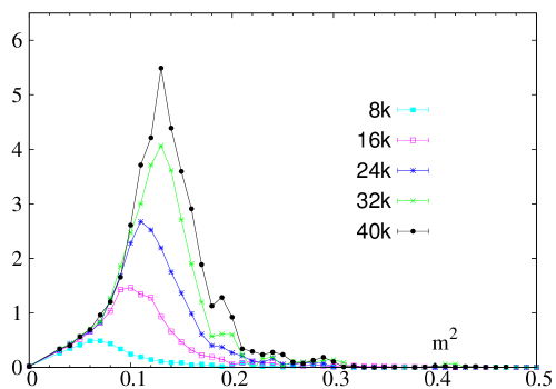
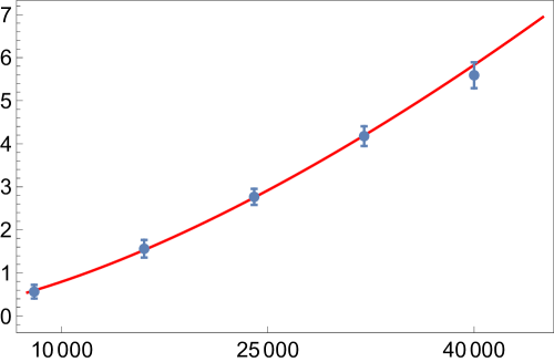
The position of the maxima permits us to estimate the transition to be located at the critical mass $m^{2}_{c}\approx 0.135\pm 0.005$. A more precise determination of the critical mass $m_{c}$ is difficult with the present numerical setup. The scaling of the maxima $H(N)$ as a function of the spacetime volume $N$ can be parametrised by

$$H(N)\sim N^{\alpha},\quad\alpha=1.48\pm 0.12$$ (14)

strongly suggesting a higher order phase transition (the fit is presented on right plot in Fig. 10 as a red line).

5 Discussion and conclusion

We analyzed spatial volume distributions $\langle n(t,m^{2})\rangle$ for CDT geometries interacting with 4 massive scalar fields. There seem to be two regimes: a small mass regime with a universal distribution identical to the distribution obtained for massless fields, i.e. for a conformal field theory with central charge $c=4$, containing a blob and a stalk, and with the blob scaling with Hausdorff dimension $D_{H}=3$. The other regime where the masses are large also has a universal distribution scaling with $D_{H}=2$ and the universal distribution is the one of pure gravity without any matter fields. Using the volume-volume correlator we located the critical mass $m_{c}^{2}$ where the transition between the two regime of different geometries takes place. The scaling of the derivative of the correlator at the critical mass $m_{c}^{2}$ as a function of system size suggests that the phase transition is of second or higher order.

We observe the same blob structure for any number $d>1$ of massless Gaussian fields, as well as for multiple critical Ising spins corresponding to $c>1$ coupled to CDT geometries. We have not observed the blobs for a single Ising spin, a single three-states Pott model or a single massless Gaussian field coupled to CDT geometries, systems which all have $c\leq 1$. Thus it is natural to conjecture that there is $c=1$ barrier also in 2d CDT/Hořava-Lifshitz quantum gravity coupled to conformal field theories, and that it is a transition associated with this barrier that we observe by changing the mass of the four Gaussian fields.

It would be very interesting if one could solve the CDT model coupled to Gaussian fields analytically. Understanding the $c=1$ barrier might help us to a better understanding of the $c=1$ barrier in quantum Liouville gravity and understanding the formation of the blobs might help us to understand better the similar phenomenon in higher dimensional CDT [16], where the appearance of the blob has been important in the attempts to define a continuum limit of lattice gravity [17, 14].

Acknowledgments. HZ is partly supported by the International PhD Projects Programme of the Foundation for Polish Science within the European Regional Development Fund of the European Union, agreement no. MPD/2009/6. JJ acknowledges the support of grant DEC-2012/06/A/ST2/00389 from the National Science Centre Poland. JA and AG acknowledge support from the ERC-Advance grant 291092, “Exploring the Quantum Universe” (EQU).

References

- [1] V.G. Knizhnik, A.M. Polyakov and A.B. Zamolodchikov, Mod. Phys. Lett. A 3 (1988) 819.
- [2] F. David, Mod. Phys. Lett. A 3 (1988) 1651.
- [3] J. Distler and H. Kawai, Nucl. Phys. B 321 (1989) 509.
-
[4]
F. David,
Nucl. Phys. B 257 (1985) 45.
A. Billoire and F. David, Phys. Lett. B 168 (1986) 279-283. -
[5]
V.A. Kazakov, A.A. Migdal and I.K. Kostov,
Phys. Lett. B 157 (1985) 295-300.
D.V. Boulatov, V.A. Kazakov, I.K. Kostov and A.A. Migdal, Nucl. Phys. B 275 (1986) 641-686. -
[6]
J. Ambjorn, B. Durhuus and J. Fröhlich,
Nucl. Phys. B 257 (1985) 433-449.
J. Ambjorn, B. Durhuus, J. Fröhlich and P. Orland, Nucl. Phys. B 270 (1986) 457-482. - [7] P. Hořava, Phys. Rev. D 79 (2009) 084008 [arXiv:0901.3775, hep-th].
- [8] J. Ambjorn, L. Glaser, Y. Sato and Y. Watabiki, Phys. Lett. B 722 (2013) 172 [arXiv:1302.6359 [hep-th]].
[9]
J. Ambjorn, B. Durhuus, T. Jonsson and G. Thorleifsson,
Nucl. Phys. B 398 (1993) 568
[hep-th/9208030].
J. Ambjorn and G. Thorleifsson, Phys. Lett. B 323 (1994) 7 [hep-th/9312157].
J. Ambjorn, G. Thorleifsson and M. Wexler, Nucl. Phys. B 439 (1995) 187 [hep-lat/9411034].
M. G. Harris and J. Ambjorn, Nucl. Phys. B 474 (1996) 575 [hep-th/9602028].
F. David, Nucl. Phys. B 487 (1997) 633 [hep-th/9610037]. - [10] J. Ambjorn, K. N. Anagnostopoulos and R. Loll, Phys. Rev. D 61 (2000) 044010 [hep-lat/9909129].
- [11] J. Ambjorn, A. Görlich, J. Jurkiewicz and H. G. Zhang, Nucl.Phys. B863 (2012) 421-434, [hep-th/1201.1590].
- [12] J. Ambjorn and R. Loll, Nucl.Phys.B 536 (1998) 407-434, [hep-th/9805108].
[13]
J. Ambjorn, K.N. Anagnostopoulos and R. Loll:
Phys. Rev. D 60 (1999) 104035 [hep-th/9904012].
J. Ambjorn, K.N. Anagnostopoulos, R. Loll and I. Pushkina, Nucl. Phys. B 807 (2009) 251 [arXiv:0806.3506, hep-lat]. -
[14]
J. Ambjorn, A. Görlich, J. Jurkiewicz and R. Loll,
Phys. Rev. Lett. 100 (2008) 091304 [arXiv:0712.2485, hep-th].
Phys. Rev. D 78 (2008) 063544 [arXiv:0807.4481, hep-th].
Phys. Lett. B 690 (2010) 420-426 [arXiv:1001.4581, hep-th]. -
[15]
J. Ambjorn, J. Jurkiewicz and R. Loll,
Phys. Rev. Lett. 93 (2004) 131301 [hep-th/0404156].
Phys. Rev. D 72 (2005) 064014 [hep-th/0505154]. Phys. Lett. B 607 (2005) 205-213 [hep-th/0411152]. -
[16]
J. Ambjorn, J. Jurkiewicz and R. Loll:
Phys. Rev. D 64 (2001) 044011 [hep-th/0011276];
Nucl.Phys.B 610 (2001), 347-382 [hep-th/0105267].
Phys. Rev. Lett. 85 (2000) 924 [hep-th/0002050]. -
[17]
J. Ambjorn, A. Goerlich, J. Jurkiewicz and R. Loll,
Phys. Rept. 519 (2012) 127
[arXiv:1203.3591 [hep-th]].
J. Ambjorn, A. Gorlich, S. Jordan, J. Jurkiewicz and R. Loll, Phys. Lett. B 690 (2010) 413 [arXiv:1002.3298 [hep-th]].
J. Ambjorn, S. Jordan, J. Jurkiewicz and R. Loll, Phys. Rev. Lett. 107 (2011) 211303 [arXiv:1108.3932 [hep-th]]. Phys. Rev. D 85 (2012) 124044 [arXiv:1205.1229 [hep-th]].