Constraining the Higgs portal
with antiprotons
Abstract
The scalar Higgs portal is a compelling model of dark matter (DM) in which a renormalizable coupling with the Higgs boson provides the connection between the visible world and the dark sector. In this paper we investigate the constraint placed on the parameter space of this model by the antiproton data. Due to the fact that the antiproton-to-proton ratio has relative less systematic uncertainties than the antiproton absolute flux, we propose and explore the possibility to combine all the available data. Following this approach, we are able to obtain stronger limits if compared with the existing literature. In particular, we show that most of the parameter space close to the Higgs resonance is ruled out by our analysis. Furthermore, by studying the reach of the future AMS-02 antiproton and antideuteron data, we argue that a DM mass of GeV offers a promising discovery potential. The method of combining all the antiproton-to-proton ratio data proposed in this paper is quite general, and can be straightforwardly applied to other models.
Keywords:
dark matter; cosmic rays; multichannel analysis; antiprotons; Higgs portal.1 Introduction
Since the discovery of the first negative proton in 1955 Segre , antiprotons have become a fundamental pillar in experimental high-energy physics, both in collider physics and astrophysics. In particular, antiprotons play a starring role in the context of indirect detection of dark matter (DM): they are copiously produced in the final stages of DM annihilations into Standard Model (SM) particles as a consequence of showering and hadronization processes. This is in particular true considering DM annihilation into hadronic channels, like for instance annihilation into . However, thanks to the electroweak radiative corrections, this is also true for DM annihilations into leptonic channels, providing that the DM mass is around the TeV scale Kachelriess:2009zy ; Ciafaloni:2010qr ; Ciafaloni:2010ti .
Furthermore, the astrophysical background plaguing this potential DM signal is relatively well understood. In a standard scenario it mostly consists in secondary antiprotons originated from the interactions of primary cosmic-ray protons, produced in supernova remnants, with the interstellar gas. For these reasons the antiproton channel is considered one of the most promising probes to shed light on the true nature of DM Bergstrom:1999jc ; Barrau:2005au ; Chardonnet:1996ca ; Bergstrom:2006tk .
However, all the experimental data collected so far show a fairly good agreement with the predictions of the astrophysical background, usually computed by means of dedicated codes such as GALPROP or DRAGON. Overturning the previous perspective, this negative results is often exploited to place strong bounds on the annihilation cross-section of DM into SM particles (see, e.g., refs. Fornengo:2013xda ; Evoli:2011id ; Cirelli:2013hv ; Asano:2012zv ; Cheung:2010ua ; Cheung:2010fu ; Garny:2011ii ; Cerdeno:2011tf ; Lavalle:2011fm ; DeSimone:2013fia ; Cirelli:2014lwa ; Bringmann:2014lpa ). Following this line, in this paper we explore the constraining power of the antiproton data considering as a benchmark example the so-called Higgs portal DM model Silveira:1985rk ; McDonald ; Burgess ; PW . Despite its simplicity, in fact, this model offers a rich phenomenology, and it provides a simple and motivated paradigm of DM.
The aim of this paper is twofold. On the one hand, we extract our bounds focusing the analysis on the experimental data describing the antiproton-to-proton ratio instead of (as customary in the literature) the absolute antiproton flux. In this way we can get rid of the systematic uncertainties that usually preclude the comparison between data taken by different experiments. On the other one, we compare, in the context of the Higgs portal model and in a wide range of DM mass, our results with the bounds obtained considering the invisible Higgs decay width and the spin-independent DM-nucleon cross-section. The purpose of this comparison is to highlight the regions of the parameter space in which the antiproton data give the most stringent limits.
This paper is organized as follows. In section 2, we briefly introduce the scalar Higgs portal model. In section 3, we discuss all the relevant aspects of our analysis; in particular, we present in detail the computation of the flux considering both the standard astrophysical background and the DM signal. In section 4 we present our results, and in section 5 we discuss future prospects. Finally, we conclude in section 6. In appendix A, we generalize our results to the fermionic Higgs portal model.
2 Setup: the scalar Higgs portal
The Lagrangian of the scalar Higgs portal model that we consider in this work has the following structure Silveira:1985rk ; McDonald ; Burgess ; PW
| (1) |
where is the SM Lagrangian, is the Higgs portal coupling, and the real field is a scalar gauge singlet with mass – after electroweak symmetry breaking – given by ; is the SM Higgs doublet with vacuum expectation value (vev) GeV.
The relevant parameter space of the model is the two-dimensional plane . After electroweak symmetry breaking the Higgs portal coupling generates the trilinear vertex , where is the physical Higgs boson; this interaction is responsible for all the phenomenological properties of the model since via this vertex the DM particle communicates with all the SM species. In this paper, we focus on the possibility that the scalar field plays the role of cold DM in the Universe.
In appendix A, we will analyze a different type of Higgs portal with fermionic DM.
2.1 Relic density
Through the exchange of the Higgs in the s-channel, two DM particles can annihilate into all the SM final states that are kinematically allowed by the value of the DM mass, . The annihilation cross-section times the relative velocity of the two annihilating DM particles takes the remarkably simple form
| (2) |
where the square of the total energy in the c.o.m. frame is . In eq. (2) is the off-shell decay width of the Higgs boson (with ), summed over all the SM final states. We use the public code HDACAY Djouadi:1997yw to compute the width . In this way we are able to include i) the NLO QCD radiative corrections to the Higgs decay into quarks and ii) the Higgs decay modes into off-shell gauge bosons. The importance of these radiative effects has been emphasized in ref. Cline:2012hg .
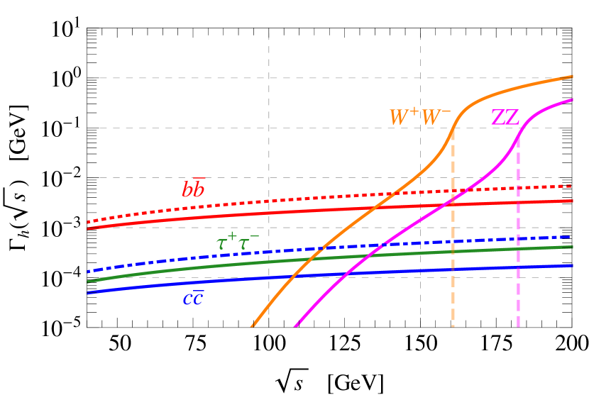
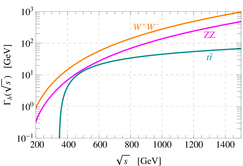
We plot in the left panel of fig. 1 the function in the energy interval GeV (left panel); we separate the most important contributions, namely the Higgs decays into SM quarks ( and ) and tau leptons as well as electroweak gauge bosons ( and ). The importance of the radiative corrections is evident from the comparison with the corresponding tree level expressions (dashed lines in fig. 1).
Going towards higher energies, there is an important issue to keep in mind. In the SM the Higgs quartic coupling is a function of the Higgs mass, i.e. and, as a consequence, . In the computation of the off-shell decay width , some electroweak corrections involving the quartic coupling are overestimated at high energy, growing like . In order to get rid of this issue, for GeV we compute analytically; we show the corresponding values for annihilation into , and in the right panel of fig. 1 in the energy interval GeV. Finally, notice that above the kinematical threshold GeV DM annihilation into two Higgses is kinematically allowed; the corresponding annihilation cross-section, however, cannot be recast in the form described by eq. (2) since, in addition to the s-channel exchange of the Higgs, also t- and u-channel diagrams in which the DM particle is exchanged contribute to the amplitude. We include this channel computing the cross-section analytically (see, e.g., ref. Guo:2010hq ).
In eq. (2) represents the on-shell decay width of the Higgs boson and it consists of two pieces, namely ; MeV is the SM contribution while is the decay width describing the process , kinematically allowed if . The explicit expression of is discussed in the context of the LHC bound (see section 2.2, eq. (8)).
The thermally averaged annihilation cross-section is given by
| (3) |
where is the temperature and are the modified Bessel functions of second kind. We numerically solve the Boltzmann equation describing the evolution of the number density of the DM particles during the expansion of the Universe, being . In terms of the yield , where is the entropy density, this equation reads
| (4) |
where
| (5) |
GeV is the Planck mass, and is the number of relativistic degrees of freedom. At the equilibrium, we have
| (6) |
where is the effective entropy.111We include in our numerical analysis the temperature dependence in and ; we extract the corresponding functions from the DarkSUSY code Gondolo:2004sc ; DarkSUSYweb . The integration of the Boltzmann equation gives the yield today, , which is related to the DM relic density through
| (7) |
The Planck collaboration has recently reported the value Ade:2013zuv ( C.L.); we compute the relic density according to eq. (7), and we impose to match the measured value.
Before proceeding, let us stress that the value of the relative velocity sets the position of the Higgs resonance during DM annihilation. From eq. (2) it follows that the pole of the Higgs propagator is given by ; at zero relative velocity, therefore, the resonant annihilation occurs at GeV, while in general it occurs at . Considering the annihilation in the early Universe – i.e. taking for definiteness – the resonance occurs at GeV.
2.2 LHC bound
If , the Higgs boson can decay into two DM particles resulting in the possibility to have a sizable invisible decay channel. In this case the invisible decay width of the Higgs is
| (8) |
The invisible branching ratio
| (9) |
is severely constrained by the current searches at the LHC ATLASinv ; CMSinv , and is excluded at 95% C.L. Falkowski:2013dza . Using eq. (9) it is straightforward to translate this bound in the parameter space , and in section 4 we will include this constraint in our analysis. To give a quantitative idea of the size of the invisible branching ratio in eq. (9), notice that for the benchmark values GeV, we have . As soon as the invisible decay channel is kinematically allowed, therefore, it can easily dominate over the SM final states even for relatively small values of the Higgs portal coupling. Notice that invisible width in eq. (8) is equal to zero for the resonant value . Therefore, it will be impossible to test this particular region using the bound on the invisible branching ratio.
2.3 Direct detection constraint
The Higgs portal interaction, through the exchange of the Higgs boson in the t-channel, provides the possibility to have a non-zero spin-independent elastic cross-section of DM on nuclei.
Integrating out the Higgs in the limit of negligible exchanged momentum, it is possible to write the following effective interactions between DM and light quarks and gluons inside the nucleus
| (10) |
with , and , where is the gluon field strength. Using this effective interaction, it is straightforward to compute the spin-independent cross-section describing the elastic DM-nucleon scattering
| (11) |
where is the DM-nucleon reduced mass, GeV is the nucleon mass, and is the Higgs-nucleon coupling Cline:2012hg . The LUX experiment has reported the strongest limit on Akerib:2013tjd . Using eq. (11) we translate this bound in the parameter space , and in section 4 we will include this constraint in our analysis.
Before proceeding, let us stress a simple but important point. The square of the momentum transferred in a typical DM-nucleus elastic scattering always satisfies the condition , with where the mass of a Xenon nucleus is GeV and for the typical recoil energy one has few keV. This simply implies that there is no resonant enhancement in elastic scatterings via the Higgs portal; as a consequence, the region with GeV where the model reproduces the correct relic abundance is beyond the present reach of direct detection experiments, and it will be covered only in the next future.
3 Antiprotons: Background vs Signal
In this section we address the properties of the transport equation describing the propagation of cosmic rays in the Galaxy. In section 3.1, we discuss the background contribution, focusing our attention mostly on astrophysical background of protons and antiprotons. In section 3.2, we illustrate the strategy that we follow in order to extract our bound on the scalar Higgs portal model.
3.1 Selection of propagation models
Considering the total luminosity injected in the Milky Way galaxy via cosmic rays, most (%) of it consists of primary protons, % of helium nuclei, a further % of heavier nuclei, and % of free electrons. In full generality, the evolution of the cosmic-ray density in the Galaxy is described by the following transport equation
| (12) | |||||
where is the number density per total unit momentum of the -th atomic species, is its momentum and is its velocity. The construction of a propagation model consists in solving eq. (12) with a certain boundary condition for all the cosmic-ray species; in this way one can compute – for a given distribution and energy spectrum of the sources – the spatial distribution and energy spectrum after propagation. Eq. (12) contains a number of free parameters to be determined. Let us discuss these parameters one by one.
-
•
For each nucleus, the source distribution and the injection index (or indices, if a break is considered). In eq. (12) these informations are encoded into the source term . Considering the contribution of the astrophysical background, describes the distribution and injection spectrum of supernova remnants Ferriere:2001rg . As far as the spectral index is concerned, we assume – following ref. Evoli:2011id – the same spectral index for all the nuclear species.
-
•
The normalization and energy dependence of the diffusion coefficient, . In eq. (12), we assume the following functional form
(13) where is the rigidity of the nucleus of charge , is the absolute normalization at reference rigidity , is the diffusion spectral index related to the turbulence of the interstellar medium, and is the scale height that controls the vertical spatial dependence, which is assumed to be exponential; the halo thickness is the height of the propagation halo where stochastic diffusion and re-acceleration take place. An additional parameter, , controls the low-energy behavior of the diffusion coefficient.
-
•
The Alfvén velocity, . It parametrizes the efficiency of the stochastic re-acceleration mechanism. In eq. (12) it enters in the explicit expression of the diffusion coefficient in momentum space, Evoli:2011id .
-
•
The convective velocity, . It is the velocity of the convective wind, if present, that may contribute to the escape of cosmic rays from the Galactic plane. The convective velocity is zero in the Galactic plane and linearly increasing with the vertical distance from the Galactic plane.
-
•
For each nucleus, the scattering cross-sections on the interstellar medium gas. The distribution of gas in the interstellar medium concentrates in the disk of the Galaxy. Its number density is denoted as , which is mainly constituted by atomic and molecular hydrogen and helium. There are two main effects. On the one hand, the -th nucleus is generated by the nuclear species with cross-section ; on the other one, the -th nucleus is destroyed by scattering on interstellar medium gas with total inelastic cross-section .
The propagation of cosmic rays can be simplified, if one takes into account only the high-energy region ( GeV). In this regime, diffusion and energy losses play an important role while other effects, such as convection and re-acceleration, are negligible. However, following this approach one is forced to neglect all the cosmic ray data at low-energy; as a consequence, the ability of constraining DM models – especially with relative low mass – decreases dramatically. In order to take advantage of all the data set, the propagation equation needs to be solved numerically without these approximation. To achieve this result, we use the public code DRAGON Evoli:2008dv ; Gaggero:2013rya , and our procedure goes as follows.
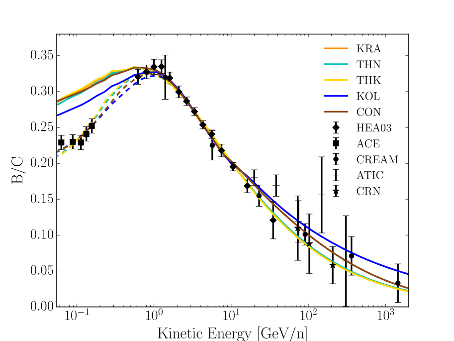
Following ref Evoli:2011id , we start from five different benchmark propagation models: KRA, KOL, CON, THK and THN. These propagation models are characterized by different halo height , slope of the diffusion coefficient , spectral index , and gradient of the convection velocity . We collect the corresponding values in table 1. KRA, KOL and CON are characterized by the same halo height ( kpc) but they describe differently turbulence effects and convection velocity. THK and THN, on the contrary, explore two extreme values for the halo height, namely kpc and kpc. Using these five benchmark propagation models, the intent is to capture a wide range of astrophysical uncertainties. For a more detailed discussion we refer the interest reader to ref. Evoli:2011id .
The second step in our analysis is to use the Boron-over-Carbon (B/C hereafter) data in order to determine – for each one of the propagation setups defined before – the remaining phenomenological parameters in eq. (12). The B/C data employed in our analysis come from the HEAO3 Engelmann:1990zz , CREAM Ahn:2008my ATIC Panov:2007fe and CRN CRN experiments. In table 1, we complete the definition of the five benchmark propagation models by minimizing the against B/C data; in this way we obtain, as output of the fitting procedure, , and the Alfvén velocity . The B/C data with energy larger than GeV are considered, and solar modulation is fixed to the value GV. The reason why we chose to define our benchmark propagation models focusing exclusively on the B/C data is that antiproton flux may originate both from astrophysical and exotic sources, while Boron and Carbon are usually generated only by astrophysical processes. Moreover, B/C represents the ratio between stable secondary cosmic-ray flux divided by the corresponding primary cosmic-ray flux, which is exactly the same as that we will use in the next step of our analysis. In the left panel of fig. 2 we show the best-fit value for the B/C flux for the five propagation models in table 1. Solid lines are obtained using GV, and the dashed line is to tune the value of in order to fit that low-energy data from the ACE collaboration. Notice that to compute , we use fixed value of the solar modulation GV to fit the other experiments data.
Finally, we can use the five propagation models in table 1 to compute the background contribution to the flux. The choice of the ratio is made with the purpose of decreasing the systematic uncertainties that come from the comparison of data taken by different experiments. As far as the antiproton flux is concerned, for instance, various experiments can have different absolute flux due to different energy calibrations, which we want to avoid. Using data describing the flux, on the contrary, we can safely combine different datasets. The data employed in our analysis come from the BESS Orito:1999re ; Asaoka:2001fv , CAPRICE Boezio:2001ac and PAMELA Adriani:2012paa experiments. At this stage, the only free parameter is the value of solar modulation; in principle, since different experiments operated at different time, we can use three independent values of – one for each experiment – in order to fit the data, and in table 1 we show the result of the corresponding fit (see caption for details).
| Model | |||||||||||
|---|---|---|---|---|---|---|---|---|---|---|---|
| (kpc) | (km s-1 kpc-1) | ( cm2 s-1) | (km s-1) | (GV) | |||||||
| KRA | 4 | 0.50 | 2.35 | 0 | 2.68 | -0.384 | 21.07 | 0.950 | 0.95 | 1.26 | 1.08 |
| THN | 0.5 | 0.50 | 2.35 | 0 | 0.32 | -0.600 | 17.87 | 0.950 | 0.88 | 1.41 | 1.26 |
| THK | 10 | 0.50 | 2.35 | 0 | 4.45 | -0.332 | 19.91 | 0.950 | 0.98 | 1.24 | 1.08 |
| KOL | 4 | 0.33 | 1.78 / 2.45 | 0 | 4.45 | 1.00 | 40.00 | 0.673 | 0.57 | 1.11 | 0.93 |
| CON | 4 | 0.60 | 1.93 / 2.35 | 50 | 0.99 | 0.786 | 40.00 | 0.19 | 0.58 | 1.00 | 0.67 |
Once the astrophysical background has been fixed, we are now in the position to discuss the contribution from DM annihilation in the Higgs portal model.

3.2 Antiproton bound on the scalar Higgs portal model
We now move to discuss the computation of the antiproton flux originated from DM annihilation in the context of the Higgs portal model.
We solve eq. (12) using as a source term
| (14) |
where is the DM density profile, the antiproton emission spectrum, i.e. the number of antiprotons per each annihilation, and is the thermally averaged annihilation cross-section times relative velocity evaluated at the present epoch. The solution of eq. 12 allows us to compute – as a function of DM mass and portal coupling, and at the location of the Earth – the antiproton flux originated from DM annihilation, . Next, we compute the local flux by combining DM contribution and astrophysical background, . Finally, by means of a fit of the data, we extract a bound on the parameter space of the scalar Higgs portal model.
We will discuss in section 4.2 the impact of different DM density profiles on the results of our analysis. In the computation of the antiproton emission spectrum, we included – consistently with the computation of the relic density – the three-body final states consisting of one on-shell and one off-shell electroweak gauge bosons. Following ref. Ciafaloni:2011sa , we made use of the PYTHIA 8.1 event generator Sjostrand:2007gs ; pythiaWS to extract these energy spectra.
4 Results
Following the approach outlined in section 3, we derived the bound on the parameter space of the scalar Higgs portal model by analyzing the antiproton-to-proton ratio data, and in this section we present and discuss our main results. We show the bound as a 3- exclusion line in the planes and . In both cases we compare the antiproton bound with the region that reproduces the correct amount of relic abundance, according to the result of the numerical analysis outlined in section 2.1. In addition, we superimpose the constraints obtained considering the invisible Higgs decay width and the spin-independent DM-nucleon elastic cross-section as described, respectively, in sections 2.2 and 2.3.
In section 4.1 we analyze the impact of different propagation models while in section 4.2 we discuss the impact of different DM density profiles.
4.1 On the impact of different propagation models
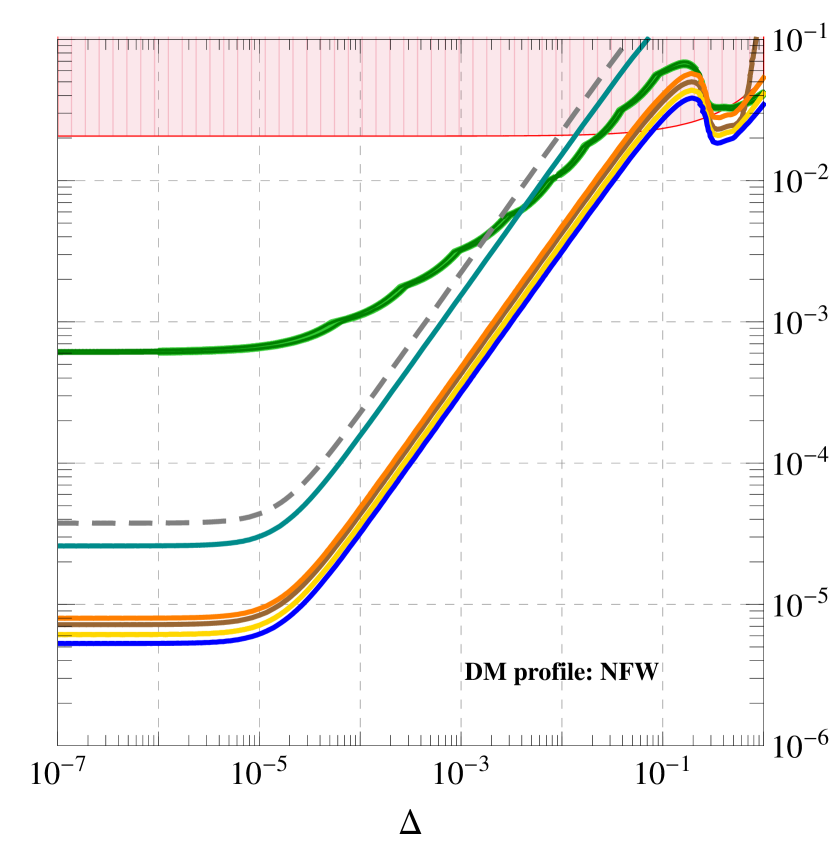
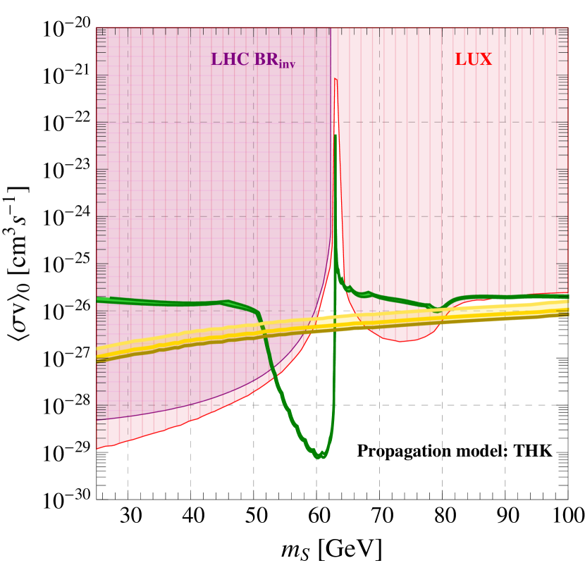
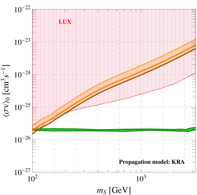
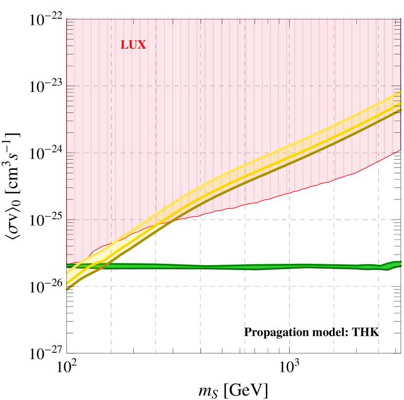
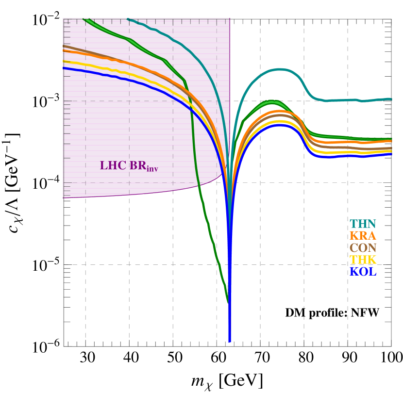
In this section, we study the antiproton bound on varying the propagation model, according to table 1. We show our results in fig. 3 and in fig. 4 where, for definiteness, we use the NFW DM density profile Navarro:1995iw (see fig. 6, eq. (15), and table 2 below).
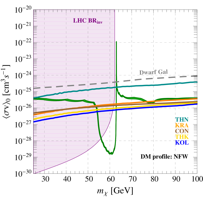
Let us start the discussion with some general comments. The region that reproduces the correct value of relic density is represented by a green strip, while the regions excluded by the LHC and LUX experiments are shaded, respectively, in purple and red. In fig. 3 we focus on small values for the DM mass, i.e. GeV, in order to emphasize the role of the antiproton bound in the region close to the Higgs resonance.
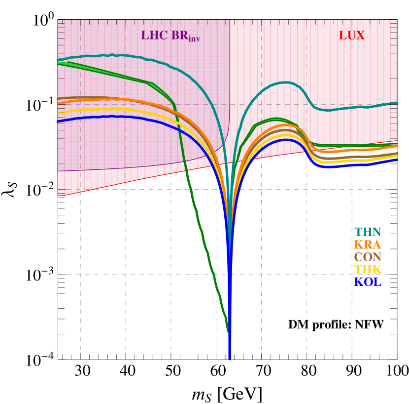
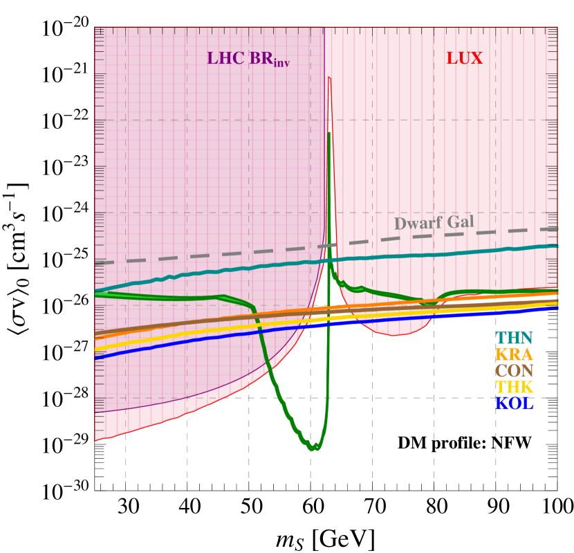
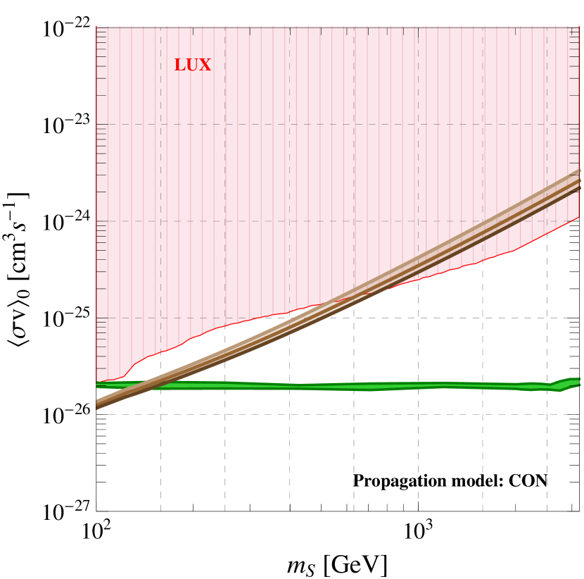
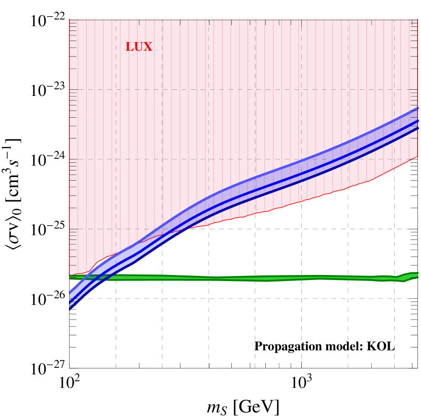
In the left panel of fig. 3 we show our results in the parameter space ; considering the green strip that reproduces the correct value of relic abundance, the resonant region is immediately recognizable because of the usual funnel-shaped form. As already discussed in section 2.1, this region extends also for values of the DM mass smaller than GeV as a consequence of thermal effects during the freeze-out epoch, and this feature clearly emerges in the plot from the result of our numerical analysis; moreover, notice that both the bound on the invisible Higgs decay width and the spin-independent DM-nucleon cross-section can not rule out this region because of the kinematical reasons discussed in sections 2.2, 2.3. In the right panel of fig. 3, we translate our analysis in the plane . Away from the resonance the value of that reproduces the observed relic abundance is close to the usual WIMP-miracle cross-section cm3s-1. Close to the resonance, on the contrary, this value is distorted by the presence of the aforementioned thermal effects that move the position of the resonance during the freeze-out epoch. In particular, we find that for the thermally averaged annihilation cross-section times relative velocity today can be as small as cm3s-1, while for we have cm3s-1. In fig. 4 we focus on large values for the DM mass, i.e. GeV. As in fig. 3, we show the constraints placed by our phenomenological analysis in the plane , left panel, and , right panel.
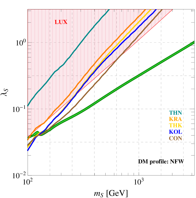
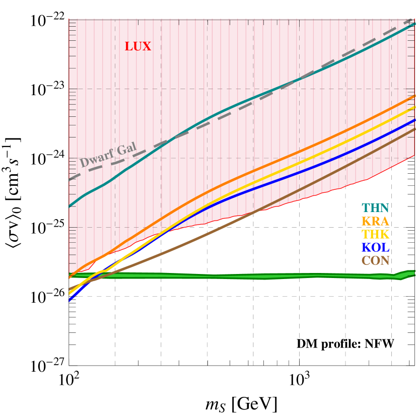
In fig. 3 and fig. 4 we show the antiproton bound that corresponds to the five propagation models defined in section 3, and we use the same color code introduced in table 1. The results of our analysis point towards the following remarks.
-
•
On a general ground, we find that the KOL, THK, CON and KRA propagation models give similar bound, while the THN propagation model places the weaker constraint. In greater detail, in the low mass region the KOL model, characterized by a strong re-acceleration, gives the strongest constraint. On the contrary in the high mass region the CON model, characterized by a strong convective wind, provides the most stringent bound. The presence of strong convective effects, in fact, hardens the antiproton flux thus leading to stronger constraints on heavier DM models Evoli:2011id . It is worth noticing that the THN model, based on a thin diffusion zone, is disfavored by recent studies on synchrotron emission, radio maps and low energy positron spectrum DiBernardo:2012zu .
-
•
In the low mass region the antiproton bound is competitive with the bound obtained from direct detection and invisible Higgs decay width. In particular, we find that the bound from antiproton is the only one able to rule out the resonant region with . Let us stress once again that this specific value for the DM mass would be otherwise inaccessible. On the one hand, in fact, the invisible Higgs branching ratio goes to zero moving towards the kinematical threshold ; on the other one, the square of the momentum transferred in a typical DM-nucleus elastic scattering always satisfies the condition , with where the mass of a Xenon nucleus is GeV and for the typical recoil energy one has few keV.
-
•
In the high mass region the antiproton bound obtained using the KOL, THK, CON and KRA propagation models is competitive with the exclusion curve traced by the LUX experiment. In particular, as clear from the right panel of fig. 4, using the KOL, THK and CON propagation models it is possible to probe the thermal cross-section up to GeV.
-
•
For comparison, we show in the right panel of figs. 3, 4 the 95% C.L. exclusion curve obtained considering the measurement of the gamma-ray flux from the dwarf spheroidal satellite galaxies of the Milky Way Ackermann:2013yva . These dwarf galaxies are some of the most DM-dominated objects known, and – because of their proximity, high DM content, and lack of astrophysical backgrounds – they are usually considered to be the most promising targets for the indirect detection of DM via gamma rays. For simplicity, in our analysis we used only the data from the Draco dwarf spheroidal galaxy since it gives the strongest constraint. Let us now describe in more detail our approach. In order to use the result of ref. Ackermann:2013yva , first we computed the gamma-ray flux from the Draco dwarf spheroidal galaxy in the Higgs portal model under scrutiny, combining all the different annihilation channels including three-body final states. Then, for each value of the DM mass, we compared the gamma-ray flux previously obtained with the 95% C.L. exclusion limit in each of the 24 energy bins analyzed in fig. 2 of ref. Ackermann:2013yva . Finally, we extracted the bound on the cross-section from the energy bin that provides the strongest constraint. We find that, both in the low- and high-mass regions, the bound from antiproton that we obtain using the KOL, THK, CON and KRA propagation models is more than one order of magnitude stronger than the bound obtained from the analysis of the gamma-ray flux measured from the Draco dwarf spheroidal galaxy. Needless to say, a more detailed analysis would require to include all the 25 dwarf spheroidal galaxies studied in ref. Ackermann:2013yva together with a more careful investigation of the systematic errors involved. This task goes well beyond the purpose of the simple estimation that we derived in this work, and will be left for future investigation.
In conclusion, we have found that the antiproton bound provides a strong constraint on the parameter space of the scalar Higgs portal model introduced in section 2. Remarkably, the constraining power of the antiproton data is comparable to the exclusion curves placed by the LHC and LUX experiments in particular for GeV. Most importantly, the antiproton bound is the only one able to rule out the Higgs resonant region for GeV. This conclusion does not strongly depend on the model used to describe the dynamics underlying the propagation of charged particle in the Galaxy; in particular, we have shown that the KOL, THK, CON and KRA propagation setups give, in magnitude, similar bounds.
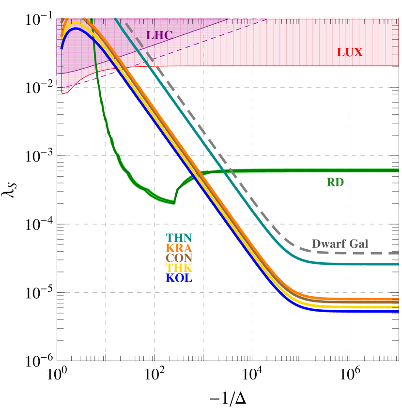
In order to stress this point we show in fig. 5, following ref. Feng:2014vea , a zoom on the Higgs resonant region. We introduce the variable , and we present our constraints in the plane . From this point of view, it is clear that the bound we get from the antiproton data is by far the most stringent if compared with LHC and LUX results. The only region left unconstrained by the antiproton bound is the small mass window with which corresponds to GeV with . In this region the position of the Higgs resonance is subject to thermal effects; as previously discussed, in this small mass window the resonant annihilation cross-section reproducing in the early Universe the correct relic abundance corresponds to an off-resonant value in today’s annihilations in the Galactic halo.
In this section we extracted the antiproton bound using the standard NFW profile in order to describe the density distribution of DM in the Galaxy. In the next section, we will discuss the impact of different DM halo profiles.
4.2 On the impact of different DM density profiles
In this section we explore the impact of different DM density profile on the analysis of the antiproton data. In addition to the NFW profile Navarro:1995iw already used in section 4.1, we repeat our analysis using the Einasto Navarro:2008kc ; Graham:2005xx and the Isothermal profile Burkert:1995yz . The former – similar to the NFW profile and characterized by a DM density distribution peaked towards the Galactic center – is favored by the latest standard numerical simulations Navarro:2003ew ; Graham:2006ae while the latter – characterized by a constant core – seems to be in agreement with the numerical simulations that include baryons, because of large exchange of angular momentum between the gas and DM particles ElZant:2003rp . We show these three DM density distributions in fig. 6 and eqs. (15, 16, 17), while in table 2 we collect the numerical values of the parameters that enter in their definitions.
![[Uncaptioned image]](/html/1412.3798/assets/x11.png)
| (15) | |||||
| (16) | |||||
| (17) |
| DM halo | [kpc] | [GeVcm-3] |
|---|---|---|
| NFW | 24.42 | 0.184 |
| Ein | 28.44 | 0.033 |
| Iso | 4.38 | 1.385 |
We show our results in fig. 7, for the low mass region, and in fig. 8, for the high mass region. In both cases we focus on the plane .


Let us start our discussion pointing out an important argument to keep in mind for the rest of the section. As a rule of thumb, one would expect that the antiproton flux from DM annihilation is larger for profiles in which the DM density is enhanced towards the Galactic center while is smaller for density distribution described by an isothermal sphere; as a consequence, one would naïvely guess that a common feature of the analysis is that the antiproton bound is always more (less) stringent for the NFW (Isothermal) profile. In general, however, this conclusion turns out to be partially incorrect. What really matters, in fact, is not the value of DM density at the Galactic center but at the position where the antiprotons – whose flux is measured on Earth – are generated. As one can easily imagine, further insights on this issue are strongly linked to the assumed propagation model, and our analysis points towards the following results.
-
•
We find that the antiproton bound obtained using the THN model, based on a very thin diffusion zone, does not significantly depend on the DM density profile, and we do not show the corresponding plot in figs. 7, 8. In the THN model, in fact, the antiproton flux from DM annihilation is dominated by local contributions where the three profiles are equivalent Evoli:2011id .
-
•
As far as the antiproton bound obtained assuming the CON propagation model is concerned, we find that also in this case the impact of different DM density distribution is moderately negligible, as shown in the upper-left panel of figs. 7, 8. As already observed in ref. Evoli:2011id , therefore, we argue that the uncertainty related to the DM distribution towards the Galactic center has a negligible effect in the CON model in which the antiproton flux from DM annihilation is dominated by local contributions.
-
•
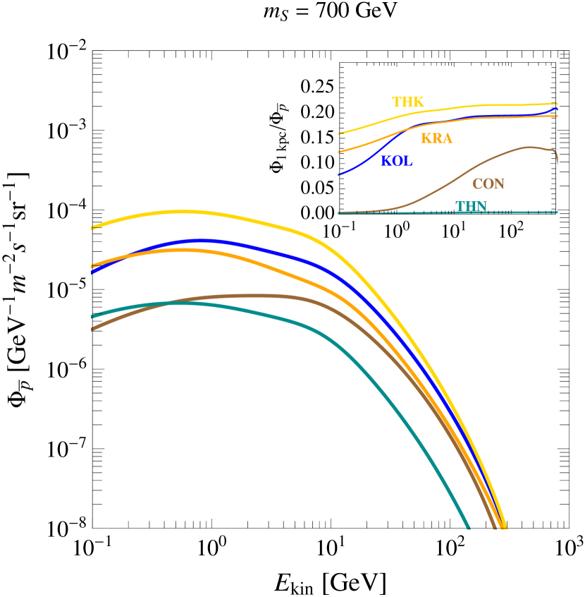
The impact of different DM density distribution is relevant considering the antiproton bound obtained using the KOL, THK and KRA propagation models. In these models, therefore, a large contribution on the antiproton flux from DM annihilation comes from non-local regions pointing towards the Galactic center where the three profiles present sizable differences, being more or less peaked. In greater detail, we find that the Isothermal (Einasto) profile gives the weaker (stronger) constraint; moreover, comparing with the NFW case, the bound obtained assuming the Isothermal density distribution has the largest deviation, while the Einasto density distribution gives a similar result. Comparing the three profiles, as done in fig. 6, we notice that in the region kpc – being r the radial distance from the Galactic center – the density distribution in both the Einasto and the NFW profiles are significantly larger than the Isothermal case; moreover, in this region the Einasto density distribution is larger if compared with the NFW one, thus reflecting the hierarchy observed in the exclusion curves. On the contrary, for kpc, the density distribution in the NFW case is larger w.r.t. the Einasto profile. All in all, we argue that in the KOL, THK and KRA propagation model the antiproton flux from DM annihilation is dominated by regions close to the Galactic center, with kpc. In order to strengthen this argument, we show in fig. 9 the local antiproton flux coming from DM annihilation and, in the inset plot, the relative contribution from a region enclosed within kpc from the Galactic center. For definiteness, we consider cm3s-1 and DM annihilation into () for GeV ( GeV).222Without solar modulation, as plotted in the left panel of fig. 9, the CON and THN models have similar flux at given DM mass ( GeV) and cross section. However, their antiproton bounds are different as shown in fig. 3. The reason is that the CON model gives harder cosmic-ray spectrum, which asks for smaller value of solar modulation. Taking properly into account the different values of solar modulation, the THN model has looser bound than the CON one. From this plot it is clear that for all the propagation models the contribution to the total antiproton flux from the inner Galactic region is at most %. Moreover, as expected, the THN and CON propagation models receive a negligible contribution from the region with kpc. The thin height of the diffusion zone and the presence of strong convective wind efficiently remove a large fraction of the antiprotons originated towards the center of the Galaxy increasing their escape probability.

In conclusion, we have shown that the role of the DM density distribution in the Galaxy plays only a relatively marginal role in our analysis, and the astrophysical uncertainties affecting the limits on the scalar Higgs portal model that one can obtain using the antiproton data are mostly dominated by the details of the propagation model.333We remind that in this paper we do not consider additional uncertainties that could affect the computation of the antiproton flux both from DM annihilation and cosmic rays. Strong outflows from the Galactic center, for instance, can carry away a lot of annihilation products thus weakening the correlation between the locally observed at Earth and the ones produced by DM annihilation; a more detailed analysis of astrophysical uncertainties can be found in ref. Evoli:2011id . Notice, moreover, that in our analysis we extract the bound on DM using a fixed value for the solar modulation potential (the one obtained from the best-fit of the background contribution, see table 1). A different approach is based on the possibility to treat this variable as a nuisance parameter in the fit, thus leading to slightly weaker constraints; a more detailed analysis along this line can be found in refs. Fornengo:2013xda ; Cirelli:2014lwa . Finally, there is an additional source of uncertainty related to the nuclear cross-sections describing the production of secondary . If introduced, this additional uncertainty will weaken the bound Fornengo:2013xda . In this regards, the antiproton data that will be released by the AMS-02 experiment will play a crucial role in order to improve the current sensitivity. In the next section, therefore, we will briefly discuss future perspectives.
5 Future perspectives
In this section we discuss some future perspectives related to our analysis. In section 5.1, we analyze the constraining power of the antiproton data that will be released by the AMS-02 experiment. In section 5.2, we analyze the antideuteron flux from DM annihilation in the scalar Higgs portal model.
5.1 AMS-02
The Alpha Magnetic Spectrometer (AMS-02) is a particle physics detector hosted on board of the International Space Shuttle, and designed to measure various cosmic-ray fluxes; thanks to this instrument, in the next future a more precise determination of the antiproton and antiproton-to-proton ratio will improve the constraints derived in this paper. To get a more concrete idea, we can simulate the prospects of this experiment by means of a set of mock data, in the energy range of (1 GeV, 450 GeV). Following ref. AMS02slides , we use a linear approximation of the AMS-02 detector energy resolution
| (18) |
DeSimone:2013fia ; Cirelli:2013hv . which determines the energy bin-size of the data. Having the bin size and the flux for each bin, the observed antiproton number can be derived as , where we take for the efficiency, m2sr for the geometrical acceptance of the instrument, and year for the reference data taking time. Since the dominant statistical uncertainty comes from the antiproton rather than the proton flux, the statistical error is approximately ; for definiteness, we fixed the systematic uncertainties to be for one-year data taking. The uncertainty at each data point is the sum in quadrature of the systematic and statistical errors. The central value of the data for each bin, , follows the predicted flux from our five benchmark propagation models, which does not contain any DM contribution. With these mock data in hand, we can study the future sensitivity of antiproton-to-proton ratio data on DM models.


In fig. 10 we show the projected bounds on the DM annihilation cross-section in the low- (left panel) and high-mass region (right panel) considering, as two extreme cases, the THN and KOL propagation models. We find that the future AMS-02 antiproton data will improve the bound for more than an order of magnitude in the high-mass region. On the contrary, in the low-mass region, our analysis show a little improvement if compared with the existing data. This is because we already exploited the full available data set, which is of reasonably good quality in the low-energy region, and goes until the lowest value of GeV, while the mock AMS-02 data starts from GeV. In the high-energy region, on the contrary, AMS-02’s resolution and luminosity are much better than the current status.
5.2 Antideuteron
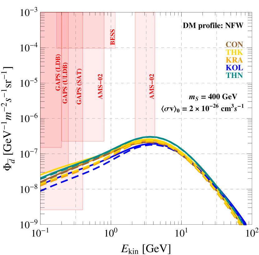
Antideuteron has been proposed in ref. Donato:1999gy as a promising indirect signal of DM annihilation in the Galactic halo. On a general ground, the annihilation of DM particles into SM hadronic channels – i.e. , , and – may produce antideuterons in the final state as a consequence of a two-step process. First – after showering, hadronization, and decay of unstable particles – a large number of antiprotons and antineutrons are produced. Second, an antiproton-antineutron pair may coalesce to form an antideuteron nucleus. The description of this process is usually addressed in the context of the so-called coalescence model. Given an antiproton and an antineutron with four-momenta and , the coalesce model approximates the probability for the formation of an antideuteron with the step function , where , and is the maximum value of relative momentum that allows to form an antideuteron bound state. In this picture, is a free parameter and its numerical value has to be extracted from experimental data (see refs. Ibarra:2012cc ; Fornengo:2013osa for a detailed discussion). In our analysis we use the results of ref. Cirelli:2010xx in order to reconstruct the antideuteron energy spectra produced by DM annihilation. These energy spectra have been obtained using MeV, and the coalescence model previously discussed has been applied studying DM annihilations event-by-event Kadastik:2009ts . Let us now move to discuss the antideuteron produced by high-energy astrophysical phenomena. The most relevant argument supporting the claim in ref. Donato:1999gy , in fact, emerges from the comparison between the antideuteron signal produced by DM annihilation and the corresponding astrophysical background. To be more precise, there are two key points to keep in mind. i) Antideuterons are produced by high-energy collisions between extragalactic cosmic rays (mostly , and He) and the interstellar gas (mostly H and He) in the Galactic disk; the corresponding cross-section is small and – most importantly – it is characterized by a relatively high kinematical threshold; for instance the energy threshold for the creation of an antideuteron from a collision of a cosmic ray proton (antiproton) with the interstellar gas is mp ( mp). Let us give a closer look to this numbers considering for definiteness the scattering between a cosmic ray proton and a proton at rest in the interstellar gas. Because of conservation of baryon number, the production of an antideuteron from a proton-proton collision requires a six-body final state, with a total energy square . On the other hand, in the rest frame of the gas, , where and are the energy and momentum of the cosmic ray proton. From these considerations, it follows that the impinging cosmic ray proton needs to have an energy mp in order to create an antideuteron. ii) The binding energy for an antideuteron is extremely low, namely MeV. This implies that antideuterons are easily destroyed, and – as a consequence – they do not have to possibility to propagate long enough in order to loose most of their energy. The astrophysical background of antideuterons with kinetic energy GeV, therefore, is expected to be extremely small. Below these kinetic energies, an antideuteron flux originated from DM annihilation may easily stand out from the astrophysical background for more than one order of magnitude.
In order to translate these qualitative statements into more quantitative results, we need to compare antideuteron background and DM signal after propagation in the Galaxy. The cross-sections describing production, elastic and inelastic scattering of antideuteron – key ingredients in order to solve the corresponding propagation equation, see eq. (12) – are not well known. Following ref. Hryczuk:2014hpa , we implemented in the DRAGON code all these cross-sections using the results of ref. Duperray:2005si , where they were extrapolated from experimental data under reasonable assumptions. In this way, we are in the position to solve numerically the propagation equation for antideuterons considering both the astrophysical background and the DM signal.
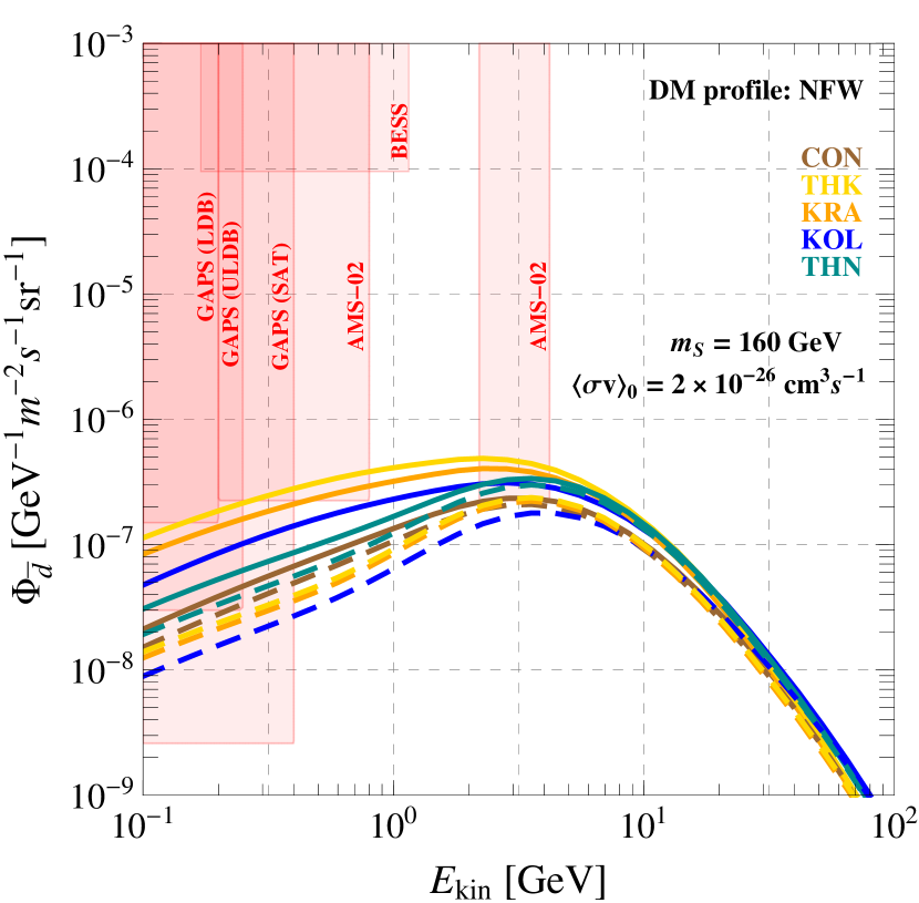
Present and future experiments – two energy bands of the AMS-02 experiment and the three phases of the General AntiParticle Spectrometer (GAPS) Mori:2001dv ; Fuke:2008zz – will increase the sensitivity of searches for cosmic-ray antideuteron over the current bound set by the BESS experiment. For the proposed sensitivities of AMS-02 and GAPS experiments we use the values from ref. Hryczuk:2014hpa . In fig. 11, we present the predictions of the scalar Higgs portal model for the antideuteron flux, comparing background and background plus DM signal hypothesis. We analyze two benchmark values for the DM mass, and we use for definiteness the NFW density profile. In the left panel of fig. 1 we take GeV, with cm3s-1. These values correspond to a DM candidate that, according to figs. 4, 8, lies close to the present bound placed by the analysis of the PAMELA antiproton data. We find that the corresponding total antideuteron flux is higher than all the experimental sensitivities of the GAPS experiment assuming the KOL, THK and KRA propagation models. Therefore in these cases, if such DM candidate is realized in Nature, we expect – in principle – a combined detection in both antideuteron and antiproton channels. For illustrative purposes, we show in the right panel of fig. 11 a different situation with GeV, cm3s-1. These values correspond to a DM candidate that, according to fig. 10, lies close to the future bound that will be placed by the analysis of the AMS-02 antiproton data. In this case, however, the total antideuteron flux will be hardly distinguishable from the astrophysical background.
6 Conclusions and outlook
In this work, we extracted a new bound on the scalar Higgs portal DM model using high-energy cosmic-ray astrophysics. In summary, the main points of our analysis are the following. First, we studied the propagation equation that governs the motion of charged particles in the Milky Way galaxy using the numerical code DRAGON. This equation depends on several free parameters that encode the astrophysical uncertainties describing the propagation of cosmic rays in the Galaxy. We fixed some of these parameters – i.e. the halo thickness, the source spectral index, the rigidity slope and the gradient of the convection velocity in the vertical direction – so to define five different propagation setups. Using the measurement of the boron-to-carbon ratio performed by the HEAO-3, ACE, CREAM, ATIC and CRN experiments, we fixed, via a minimization procedure, the remaining ones – i.e. the normalization of the diffusion coefficient, the Alfvén velocity and the low-energy diffusion index. Second, using the propagation setups fixed by the B/C data, we predicted the background contribution to the antiproton-to-proton ratio. Finally, we computed the antiproton flux from DM annihilation in the Higgs portal model including three-body final states and QCD radiative corrections; using the antiproton-to-proton ratio previously discussed, and combining background and DM signal, we extracted 3- bound on the parameter space of the model. The use of the antiproton-to-proton ratio allowed us to combine different experiments, namely PAMELA, BESS and CAPRICE data. In the antiproton-to-proton ratio, in fact, several systematic effects that plague the comparison between different experiments – as for instance different energy calibration – are integrated out. We compared our antiproton bound with the constraints coming from the LUX and LHC experiments considering – respectively – direct detection of DM particles and the invisible decay width of the Higgs boson. At the same time, we required to reproduce the observed amount of relic density.
We found that the antiproton bound is competitive; in particular, it provides the most stringent constraint on the model in the mass range GeV for most of the analyzed propagation setups. Most importantly, the antiproton bound is the only one able to put in significant tension the resonant region , otherwise of difficult access to direct detection and collider searches.
In our analysis, we investigated the impact of astrophysical uncertainties related to different propagation setups and different models for the DM density distribution in the Galaxy. Moreover, we discussed future perspectives using a set of mock data in order to simulate those that will be released in the near future by the AMS-02 experiment. Finally, we highlighted in the context of the scalar Higgs portal model the role of the antideuteron channel as an important indirect detection observable able to provide a signature of annihilating DM.
Acknowledgements.
We thank Daniele Gaggero, Andrzej Hryczuk and in particular Piero Ullio for useful discussions and advices. The work of A.U. is supported by the ERC Advanced Grant n∘ , “Electroweak Symmetry Breaking, Flavour and Dark Matter: One Solution for Three Mysteries” (DaMeSyFla).Appendix A Spin-1/2 Higgs portal
In this Appendix we focus on the following fermionic Higgs portal Lagrangian LopezHonorez:2012kv
| (19) |
where is Dirac field playing the role of DM. The parity-conserving interaction is severely constrained by direct detection experiments Kanemura:2010sh ; moreover the annihilation cross-section suffers from a p-wave suppression (see, e.g., Ref. Huang:2013apa ) that makes it undetectable for any indirect detection experiment. The bound discussed in this paper, therefore, does not apply on this interaction. The parity-violating interaction , on the contrary, induces a velocity-suppressed spin-independent elastic cross-section on nuclei but an unsuppressed annihilation cross-section. As a consequence we expect that the bound from antiprotons, in absence of a significant direct detection signal, is the strongest constraint that can be placed on the parameter space of this model.
Compared with eq. (2), the annihilation cross-section times relative velocity is
| (20) |
with , and
| (21) |
The phenomenological analysis proceeds parallel to the scalar case.
References
- (1) O. Chamberlain, E. Segre, C. Wiegand and T. Ypsilantis, Phys. Rev. 100, 947 (1955).
- (2) M. Kachelriess, P. D. Serpico and M. A. Solberg, Phys. Rev. D 80, 123533 (2009) [arXiv:0911.0001[hep-ph]].
- (3) P. Ciafaloni and A. Urbano, Phys. Rev. D 82, 043512 (2010) [arXiv:1001.3950[hep-ph]].
- (4) P. Ciafaloni, D. Comelli, A. Riotto, F. Sala, A. Strumia and A. Urbano, JCAP 1103, 019 (2011) [arXiv:1009.0224[hep-ph]].
- (5) L. Bergstrom, J. Edsjo and P. Ullio, Astrophys. J. 526, 215 (1999) [astro-ph/9902012].
- (6) A. Barrau, P. Salati, G. Servant, F. Donato, J. Grain, D. Maurin and R. Taillet, Phys. Rev. D 72, 063507 (2005) [astro-ph/0506389].
- (7) P. Chardonnet, G. Mignola, P. Salati and R. Taillet, Phys. Lett. B 384, 161 (1996) [astro-ph/9606174].
- (8) L. Bergstrom, J. Edsjo, M. Gustafsson and P. Salati, JCAP 0605, 006 (2006) [astro-ph/0602632].
- (9) N. Fornengo, L. Maccione and A. Vittino, JCAP 1404, 003 (2014) [arXiv:1312.3579[hep-ph]].
- (10) C. Evoli, I. Cholis, D. Grasso, L. Maccione and P. Ullio, Phys. Rev. D 85, 123511 (2012) [arXiv:1108.0664[astro-ph.HE]].
- (11) M. Cirelli and G. Giesen, JCAP 1304, 015 (2013) [arXiv:1301.7079[hep-ph]].
- (12) M. Asano, T. Bringmann, G. Sigl and M. Vollmann, Phys. Rev. D 87, no. 10, 103509 (2013) [arXiv:1211.6739[hep-ph]].
- (13) K. Cheung, P. Y. Tseng and T. C. Yuan, JCAP 1101, 004 (2011) [arXiv:1011.2310[hep-ph]].
- (14) K. Cheung, J. Song and P. Y. Tseng, JCAP 1009, 023 (2010) [arXiv:1007.0282[hep-ph]].
- (15) M. Garny, A. Ibarra and S. Vogl, JCAP 1204, 033 (2012) [arXiv:1112.5155[hep-ph]].
- (16) D. G. Cerdeno, T. Delahaye and J. Lavalle, Nucl. Phys. B 854, 738 (2012) [arXiv:1108.1128[hep-ph]].
- (17) J. Lavalle, J. Phys. Conf. Ser. 375 (2012) 012032 [arXiv:1112.0678[astro-ph.HE]].
- (18) A. De Simone, A. Riotto and W. Xue, JCAP 1305, 003 (2013) [JCAP 1305, 003 (2013)] [arXiv:1304.1336 [hep-ph]].
- (19) M. Cirelli, D. Gaggero, G. Giesen, M. Taoso and A. Urbano, arXiv:1407.2173[hep-ph].
- (20) T. Bringmann, M. Vollmann and C. Weniger, Phys. Rev. D 90, 123001 (2014) [arXiv:1406.6027[astro-ph.HE]].
- (21) V. Silveira and A. Zee, Phys. Lett. B 161, 136 (1985).
- (22) J. McDonald, Phys. Rev. D 50, 3637 (1994) [hep-ph/0702143].
- (23) C. P. Burgess, M. Pospelov and T. ter Veldhuis, Nucl. Phys. B 619, 709 (2001) [hep-ph/0011335].
- (24) B. Patt and F. Wilczek, hep-ph/0605188.
- (25) A. Djouadi, J. Kalinowski and M. Spira, Comput. Phys. Commun. 108, 56 (1998) [hep-ph/9704448].
- (26) J. M. Cline and K. Kainulainen, JCAP 1301, 012 (2013) [arXiv:1210.41968].
- (27) W. -L. Guo and Y. -L. Wu, JHEP 1010, 083 (2010) [arXiv:1006.2518].
- (28) P. Gondolo, J. Edsjo, P. Ullio, L. Bergstrom, M. Schelke and E. A. Baltz, JCAP 0407, 008 (2004) [astro-ph/0406204].
- (29) P. Gondolo, J. Edsjö, P. Ullio, L. Bergström, M. Schelke, E.A. Baltz, T. Bringmann and G. Duda, DarkSUSY webpage.
- (30) P. A. R. Ade et al. [Planck Collaboration], arXiv:1303.5076.
- (31) ATLAS Collaboration, ATLAS-CONF-2013-011.
- (32) CMS Collaboration, HIG-13-028.
- (33) A. Falkowski, F. Riva and A. Urbano, JHEP 1311, 111 (2013) [arXiv:1303.1812].
- (34) D. S. Akerib et al. [LUX Collaboration] arXiv:1310.8214.
- (35) K. M. Ferriere, Rev. Mod. Phys. 73, 1031 (2001) [astro-ph/0106359].
- (36) C. Evoli, D. Gaggero, D. Grasso and L. Maccione, JCAP 0810, 018 (2008) [arXiv:0807.4730[astro-ph]].
- (37) D. Gaggero, L. Maccione, G. Di Bernardo, C. Evoli and D. Grasso, Phys. Rev. Lett. 111, no. 2, 021102 (2013) [arXiv:1304.6718[astro-ph.HE]].
- (38) J. J. Engelmann, P. Ferrando, A. Soutoul, P. Goret and E. Juliusson, Astron. Astrophys. 233 (1990) 96.
- (39) H. S. Ahn, P. S. Allison, M. G. Bagliesi, J. J. Beatty, G. Bigongiari, P. J. Boyle, T. J. Brandt and J. T. Childers et al., Astropart. Phys. 30 (2008) 133 [arXiv:0808.1718].
- (40) A. D. Panov, N. V. Sokolskaya, J. H. Adams, Jr., H. S. Ahn, G. L. Bashindzhagyan, K. E. Batkov, J. Chang and M. Christl et al., arXiv:0707.4415.
- (41) D. Mueller, S. P. Swordy, P. Meyer, J. L’Heureux and J. M. Grunsfeld, Astrophysical Journal 374 (1991) 356
- (42) S. Orito et al. [BESS Collaboration], Phys. Rev. Lett. 84, 1078 (2000) [astro-ph/9906426].
- (43) Y. Asaoka, Y. Shikaze, K. Abe, K. Anraku, M. Fujikawa, H. Fuke, M. Imori and S. Haino et al., Phys. Rev. Lett. 88, 051101 (2002) [astro-ph/0109007].
- (44) M. Boezio et al. [WiZard/CAPRICE Collaboration], Astrophys. J. 561, 787 (2001) [astro-ph/0103513].
- (45) O. Adriani, G. A. Bazilevskaya, G. C. Barbarino, R. Bellotti, M. Boezio, E. A. Bogomolov, V. Bonvicini and M. Bongi et al., JETP Lett. 96, 621 (2013) [Pisma Zh. Eksp. Teor. Fiz. 96, 693 (2012)].
- (46) P. Ciafaloni, M. Cirelli, D. Comelli, A. De Simone, A. Riotto and A. Urbano, JCAP 1106, 018 (2011) [arXiv:1104.2996].
- (47) T. Sjostrand, S. Mrenna and P. Z. Skands, Comput. Phys. Commun. 178, 852 (2008) [arXiv:0710.3820].
- (48) PYTHIA 8.1 web-page.
- (49) J. F. Navarro, C. S. Frenk and S. D. M. White, Astrophys. J. 462, 563 (1996) [astro-ph/9508025].
- (50) G. Di Bernardo, C. Evoli, D. Gaggero, D. Grasso and L. Maccione, JCAP 1303, 036 (2013) [arXiv:1210.4546].
- (51) M. Ackermann et al. [Fermi-LAT Collaboration], Phys. Rev. D 89, 042001 (2014) [arXiv:1310.0828].
- (52) L. Feng, S. Profumo and L. Ubaldi, arXiv:1412.1105[hep-ph].
- (53) J. F. Navarro, A. Ludlow, V. Springel, J. Wang, M. Vogelsberger, S. D. M. White, A. Jenkins and C. S. Frenk et al., arXiv:0810.1522.
- (54) A. W. Graham, D. Merritt, B. Moore, J. Diemand and B. Terzic, Astron. J. 132, 2685 (2006) [astro-ph/0509417].
- (55) A. Burkert, IAU Symp. 171, 175 (1996) [Astrophys. J. 447, L25 (1995)] [astro-ph/9504041].
- (56) J. F. Navarro, E. Hayashi, C. Power, A. Jenkins, C. S. Frenk, S. D. M. White, V. Springel and J. Stadel et al., Mon. Not. Roy. Astron. Soc. 349, 1039 (2004) [astro-ph/0311231].
- (57) A. W. Graham, D. Merritt, B. Moore, J. Diemand and B. Terzic, Astron. J. 132, 2701 (2006) [astro-ph/0608613].
- (58) A. A. El-Zant, Y. Hoffman, J. Primack, F. Combes and I. Shlosman, Astrophys. J. 607, L75 (2004) [astro-ph/0309412].
- (59) S. Ting, “The Alpha Magnetic Spectrometer Experiment on the International Space Station”, talk at SpacePart12 - The 4th International Conference on Particle and Fundamental Physics in Space.
- (60) F. Donato, N. Fornengo and P. Salati, Phys. Rev. D 62, 043003 (2000) [hep-ph/9904481].
- (61) A. Ibarra and S. Wild, JCAP 1302, 021 (2013) [arXiv:1209.5539].
- (62) N. Fornengo, L. Maccione and A. Vittino, JCAP 1309, 031 (2013) [arXiv:1306.4171].
- (63) M. Cirelli, G. Corcella, A. Hektor, G. Hutsi, M. Kadastik, P. Panci, M. Raidal and F. Sala et al., JCAP 1103, 051 (2011) [Erratum-ibid. 1210, E01 (2012)] [arXiv:1012.4515].
- (64) M. Kadastik, M. Raidal and A. Strumia, Phys. Lett. B 683, 248 (2010) [arXiv:0908.1578].
- (65) A. Hryczuk, I. Cholis, R. Iengo, M. Tavakoli and P. Ullio, arXiv:1401.6212.
- (66) R. Duperray, B. Baret, D. Maurin, G. Boudoul, A. Barrau, L. Derome, K. Protasov and M. Buenerd, Phys. Rev. D 71, 083013 (2005) [astro-ph/0503544].
- (67) K. Mori, C. J. Hailey, E. A. Baltz, W. W. Craig, M. Kamionkowski, W. T. Serber and P. Ullio, Astrophys. J. 566, 604 (2002) [astro-ph/0109463].
- (68) H. Fuke, J. E. Koglin, T. Yoshida, T. Aramaki, W. W. Craig, L. Fabris, F. Gahbauer and C. J. Hailey et al., Adv. Space Res. 41, 2056 (2008).
- (69) L. Lopez-Honorez, T. Schwetz and J. Zupan, Phys. Lett. B 716, 179 (2012) [arXiv:1203.2064].
- (70) S. Kanemura, S. Matsumoto, T. Nabeshima and N. Okada, Phys. Rev. D 82, 055026 (2010) [arXiv:1005.5651].
- (71) W. C. Huang, A. Urbano and W. Xue, JCAP 1404 (2014) 020 [arXiv:1310.7609[hep-ph]].