Distinguishing cause from effect using observational data: methods and benchmarks

Abstract

The discovery of causal relationships from purely observational data is a fundamental problem in science. The most elementary form of such a causal discovery problem is to decide whether $X$ causes $Y$ or, alternatively, $Y$ causes $X$, given joint observations of two variables $X,Y$. An example is to decide whether altitude causes temperature, or vice versa, given only joint measurements of both variables. Even under the simplifying assumptions of no confounding, no feedback loops, and no selection bias, such bivariate causal discovery problems are challenging. Nevertheless, several approaches for addressing those problems have been proposed in recent years. We review two families of such methods: Additive Noise Methods (ANM) and Information Geometric Causal Inference (IGCI). We present the benchmark CauseEffectPairs that consists of data for 100 different cause-effect pairs selected from 37 datasets from various domains (e.g., meteorology, biology, medicine, engineering, economy, etc.) and motivate our decisions regarding the “ground truth” causal directions of all pairs. We evaluate the performance of several bivariate causal discovery methods on these real-world benchmark data and in addition on artificially simulated data. Our empirical results on real-world data indicate that certain methods are indeed able to distinguish cause from effect using only purely observational data, although more benchmark data would be needed to obtain statistically significant conclusions. One of the best performing methods overall is the additive-noise method originally proposed by Hoyer et al. (2009), which obtains an accuracy of 63 $\pm$ 10 % and an AUC of 0.74 $\pm$ 0.05 on the real-world benchmark. As the main theoretical contribution of this work we prove the consistency of that method.

Keywords: Causal discovery, additive noise, information-geometric causal inference, cause-effect pairs, benchmarks

1 Introduction

An advantage of having knowledge about causal relationships rather than statistical associations is that the former enables prediction of the effects of actions that perturb the observed system. Knowledge of cause and effect can also have implications on the applicability of semi-supervised learning and covariate shift adaptation (Schölkopf et al., 2012). While the gold standard for identifying causal relationships is controlled experimentation, in many cases, the required experiments are too expensive, unethical, or technically impossible to perform. The development of methods to identify causal relationships from purely observational data therefore constitutes an important field of research.

An observed statistical dependence between two variables $X$, $Y$ can be explained by a causal influence from $X$ to $Y$, a causal influence from $Y$ to $X$, a possibly unobserved common cause that influences both $X$ and $Y$ (“confounding”, see e.g., Pearl, 2000), a possibly unobserved common effect of $X$ and $Y$ that is conditioned upon in data acquisition (“selection bias”, see e.g., Pearl, 2000), or combinations of these. Most state-of-the-art causal discovery algorithms that attempt to distinguish these cases based on observational data require that $X$ and $Y$ are part of a larger set of observed random variables influencing each other. For example, in that case, and under a genericity condition called “faithfulness”, conditional independences between subsets of observed variables allow one to draw partial conclusions regarding their causal relationships (Spirtes et al., 2000; Pearl, 2000; Richardson and Spirtes, 2002; Zhang, 2008).

In this article, we focus on the bivariate case, assuming that only two variables, say $X$ and $Y$, have been observed. We simplify the causal discovery problem considerably by assuming no confounding, no selection bias and no feedback. We study how to distinguish $X$ causing $Y$ from $Y$ causing $X$ using only purely observational data, i.e., a finite i.i.d. sample drawn from the joint distribution $\mathbb{P}_{X,Y}$. As an example, consider the data visualized in Figure 1. The question is: does $X$ cause $Y$, or does $Y$ cause $X$? The true answer is “$X$ causes $Y$”, as here $X$ is the altitude of weather stations and $Y$ is the mean temperature measured at these weather stations (both in arbitrary units). In the absence of knowledge about the measurement procedures that the variables correspond with, one can try to exploit the subtle statistical patterns in the data in order to find the causal direction. This challenge of distinguishing cause from effect using only observational data has attracted increasing interest recently (Mooij and Janzing, 2010; Guyon et al., 2010, 2014). Approaches to causal discovery based on conditional independences do not work here, as $X$ and $Y$ are typically dependent, and there are no other observed variables to condition on.

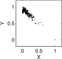
Figure 1: Example of a bivariate causal discovery task: decide whether $X$ causes $Y$, or $Y$ causes $X$, using only the observed data (visualized here as a scatter plot).

A variety of causal discovery methods has been proposed in recent years (Friedman and Nachman, 2000; Kano and Shimizu, 2003; Shimizu et al., 2006; Sun et al., 2006, 2008; Hoyer et al., 2009; Mooij et al., 2009; Zhang and Hyvärinen, 2009; Janzing et al., 2010; Mooij et al., 2010; Daniušis et al., 2010; Mooij et al., 2011; Shimizu et al., 2011; Janzing et al., 2012; Hyvärinen and Smith, 2013; Peters and Bühlmann, 2014; Kpotufe et al., 2014; Nowzohour and Bühlmann, 2015; Sgouritsa et al., 2015) that were claimed to be able to solve this task under certain assumptions. All these approaches exploit the complexity of the marginal and conditional probability distributions, in one way or the other. On an intuitive level, the idea is that the factorization of the joint density $p_{C,E}(c,e)$ of cause $C$ and effect $E$ into $p_{C}(c)p_{E\,|\,C}(e\,|\,c)$ typically yields models of lower total complexity than the alternative factorization into $p_{E}(e)p_{C\,|\,E}(c\,|\,e)$. Although this idea is intuitively appealing, it is not clear how to define complexity. If “complexity” and “information” are measured by Kolmogorov complexity and algorithmic information, respectively, as in (Janzing and Schölkopf, 2010; Lemeire and Janzing, 2013), one can show that the statement “$p_{C}$ contains no information about $p_{E\,|\,C}$” implies that the sum of the complexities of $p_{C}$ and $p_{E\,|\,C}$ cannot be greater than the sum of the complexities of $p_{E}$ and $p_{C\,|\,E}$. Some approaches, instead, define certain classes of “simple” conditionals, e.g., Additive Noise Models (Hoyer et al., 2009) and second-order exponential models (Sun et al., 2006; Janzing et al., 2009), and infer $X$ to be the cause of $Y$ whenever $\mathbb{P}_{Y\,|\,X}$ is from this class (and $\mathbb{P}_{X\,|\,Y}$ is not). Another approach that employs complexity in a more implicit way postulates that $\mathbb{P}_{C}$ contains no information about $\mathbb{P}_{E\,|\,C}$ (Janzing et al., 2012).

Despite the large number of methods for bivariate causal discovery that has been proposed over the last few years, their practical performance has not been studied very systematically (although domain-specific studies have been performed, see (Smith et al., 2011; Statnikov et al., 2012)). The present work attempts to address this by presenting benchmark data and reporting extensive empirical results on the performance of various bivariate causal discovery methods. Our main contributions are fourfold:

• We review two families of bivariate causal discovery methods, Additive Noise Methods (ANM) (originally proposed by Hoyer et al., 2009), and Information Geometric Causal Inference (IGCI) (originally proposed by Daniušis et al., 2010).

• We present a detailed description of the benchmark CauseEffectPairs that we collected over the years for the purpose of evaluating bivariate causal discovery methods. It currently consists of data for 100 different cause-effect pairs selected from 37 datasets from various domains (e.g., meteorology, biology, medicine, engineering, economy, etc.).

• We report the results of extensive empirical evaluations of the performance of several members of the ANM and IGCI families, both on artificially simulated data as well as on the CauseEffectPairs benchmark.

• We prove the consistency of the original implementation of ANM that was proposed by Hoyer et al. (2009).

The CauseEffectPairs benchmark data are provided on our website (Mooij et al., 2014). In addition, all the code (including the code to run the experiments and create the figures) is provided on the first author’s homepage under an open source license to allow others to reproduce and build on our work.

The structure of this article is somewhat unconventional, as it partially consists of a review of existing methods, but it also contains new theoretical and empirical results. We will start in the next subsection by giving a more rigorous definition of the causal discovery task we consider in this article. In Section 2 we give a review of ANM, an approach based on the assumed additivity of the noise, and describe various ways of implementing this idea for bivariate causal discovery. In Appendix A we provide a proof for the consistency of the original ANM implementation that was proposed by Hoyer et al. (2009). In Section 3, we review IGCI, a method that exploits the independence of the distribution of the cause and the functional relationship between cause and effect. This method is designed for the deterministic (noise-free) case, but has been reported to work on noisy data as well. Section 4 gives more details on the experiments that we have performed, the results of which are reported in Section 5. Appendix D describes the CauseEffectPairs benchmark data set that we used for assessing the accuracy of various methods. We conclude in Section 6.

1.1 Problem setting

In this subsection, we formulate the problem of interest central to this work. We tried to make this section as self-contained as possible and hope that it also appeals to readers who are not familiar with the terminology in the field of causality. For more details, we refer the reader to (Pearl, 2000).

Suppose that $X,Y$ are two random variables with joint distribution $\mathbb{P}_{X,Y}$. This observational distribution corresponds to measurements of $X$ and $Y$ in an experiment in which $X$ and $Y$ are both (passively) observed. If an external intervention (i.e., from outside the system under consideration) changes some aspect of the system, then in general, this may lead to a change in the joint distribution of $X$ and $Y$. In particular, we will consider a perfect intervention “$\mathrm{do}(x)$” (or more explicitly: “$\mathrm{do}(X=x)$”) that forces the variable $X$ to have the value $x$, and leaves the rest of the system untouched. We denote the resulting interventional distribution of $Y$ as $\mathbb{P}_{Y\,|\,\mathrm{do}(x)}$, a notation inspired by Pearl (2000). This interventional distribution corresponds to the distribution of $Y$ in an experiment in which $X$ has been set to the value $x$ by the experimenter, after which $Y$ is measured. Similarly, we may consider a perfect intervention $\mathrm{do}(y)$ that forces $Y$ to have the value $y$, leading to the interventional distribution $\mathbb{P}_{X\,|\,\mathrm{do}(y)}$ of $X$.

For example, $X$ and $Y$ could be binary variables corresponding to whether the battery of a car is empty, and whether the start engine of the car is broken. Measuring these variables in many cars, we get an estimate of the joint distribution $\mathbb{P}_{X,Y}$. The marginal distribution $\mathbb{P}_{X}$, which only considers the distribution of $X$, can be obtained by integrating the joint distribution over $Y$. The conditional distribution $\mathbb{P}_{X\,|\,Y=0}$ corresponds with the distribution of $X$ for the cars with a broken start engine (i.e., those cars for which we observe that $Y=0$). The interventional distribution $\mathbb{P}_{X\,|\,\mathrm{do}(Y=0)}$, on the other hand, corresponds with the distribution of $X$ after destroying the start engines of all cars (i.e., after actively setting $Y=0$). Note that the distributions $\mathbb{P}_{X},\mathbb{P}_{X\,|\,Y=0},\mathbb{P}_{X\,|\,\mathrm{do}(Y=0)}$ may all be different.

In the absence of selection bias, we define:

Definition 1

We say that $X$ causes $Y$ if  $\mathbb{P}_{Y\,|\,\mathrm{do}(x)}\neq\mathbb{P}_{Y\,|\,\mathrm{do}(x^{\prime})}$ for some $x,x^{\prime}$.

Causal relations can be cyclic, i.e., $X$ causes $Y$ and $Y$ also causes $X$. For example, an increase of the global temperature causes sea ice to melt, which causes the temperature to rise further (because ice reflects more sun light).

In the context of multiple variables $X_{1},\dots,X_{p}$ with $p\geq 2$, we define direct causation in the absence of selection bias as follows:

Definition 2

$X_{i}$ is a direct cause of $X_{j}$ with respect to $X_{1},\dots,X_{p}$ if

$$\mathbb{P}_{X_{j}\,|\,\mathrm{do}(X_{i}=x,\bm{X}_{\setminus ij}=\bm{c})}\neq\mathbb{P}_{X_{j}\,|\,\mathrm{do}(X_{i}=x^{\prime},\bm{X}_{\setminus ij}=\bm{c})}$$

for some $x,x^{\prime}$ and some $\bm{c}$, where $\bm{X}_{\setminus ij}:=X_{\{1,\dots,p\}\setminus\{i,j\}}$ are all other variables besides $X_{i},X_{j}$.

In words: $X$ is a direct cause of $Y$ with respect to a set of variables under consideration if $Y$ depends on the value we force $X$ to have in a perfect intervention, while fixing all other variables. The intuition is that a direct causal relation of $X$ on $Y$ is not mediated via the other variables. The more variables one considers, the harder it becomes experimentally to distinguish direct from indirect causation, as one has to keep more variables fixed.

We may visualize direct causal relations in a causal graph:

Definition 3

The causal graph $\mathcal{G}$ has variables $X_{1},\dots,X_{p}$ as nodes, and a directed edge from $X_{i}$ to $X_{j}$ if and only if $X_{i}$ is a direct cause of $X_{j}$ with respect to $X_{1},\dots,X_{p}$.

Note that this definition allows for cyclic causal relations. In contrast with the typical assumption in the causal discovery literature, we do not assume here that the causal graph is necessarily a Directed Acyclic Graph (DAG).

If $X$ causes $Y$, we generically have that $\mathbb{P}_{Y\,|\,\mathrm{do}(x)}\neq\mathbb{P}_{Y}$. Figure 2 illustrates how various causal relationships between $X$ and $Y$ (and at most one other variable) generically give rise to different (in)equalities between marginal, conditional, and interventional distributions involving $X$ and $Y$.

Returning to the example of the empty batteries ($X$) and broken start engines ($Y$), it seems reasonable to assume that these two variables are not causally related and case (c) in Figure 2 would apply, and therefore $X$ and $Y$ must be statistically independent.

In order to illustrate case (f), let us introduce a third binary variable, $S$, which measures whether the car starts or not. If the data acquisition is done by a car mechanic who only considers cars that do not start ($S=0$), then we are in case (f): conditioning on the common effect $S$ of $X$ and $Y$ leads to selection bias, i.e., $X$ and $Y$ are statistically dependent when conditioning on $S$ (even though they are not directly causally related). Indeed, if we know that a car doesn’t start, then learning that the battery is not empty makes it much more likely that the start engine is broken.

Another way in which two variables that are not directly causally related can still be statistically dependent is case (e), i.e., if they have a common cause. As an example, take for $X$ the number of stork breeding pairs (per year) and for $Y$ the number of human births (per year) in a country. Data has been collected for different countries and shows a significant correlation between $X$ and $Y$ (Matthews, 2000). Few people nowadays believe that storks deliver babies, or the other way around, and therefore it seems reasonable to assume that $X$ and $Y$ are not directly causally related. One obvious confounder ($Z$ in Figure 2(e)) that may explain the observed dependence between $X$ and $Y$ is land area.

When data from all (observational and interventional) distributions are available, it becomes straightforward in principle to distinguish the six cases in Figure 2 simply by checking which (in)equalities in Figure 2 hold. In practice, however, we often only have data from the observational distribution $\mathbb{P}_{X,Y}$ (for example, because intervening on stork population or human birth rate is impractical). Can we then still infer the causal relationship between $X$ and $Y$? If, under certain assumptions, we can decide upon the causal direction, we say that the causal direction is identifiable from the observational distribution (and our assumptions).

In this work, we will simplify matters considerably by considering only (a) and (b) in Figure 2 as possibilities. In other words, we assume that $X$ and $Y$ are dependent (i.e., $\mathbb{P}_{X,Y}\neq\mathbb{P}_{X}\mathbb{P}_{Y}$), there is no confounding (common cause of $X$ and $Y$), no selection bias (common effect of $X$ and $Y$ that is implicitly conditioned on), and no feedback between $X$ and $Y$ (a two-way causal relationship between $X$ and $Y$). Inferring the causal direction between $X$ and $Y$, i.e., deciding which of the two cases (a) and (b) holds, using only the observational distribution $\mathbb{P}_{X,Y}$ is the challenging task that we consider in this work.

Figure 2: Several possible causal relationships between two observed variables $X,Y$ and a single latent variable: (a) $X$ causes $Y$; (b) $Y$ causes $X$; (c) $X,Y$ are not causally related; (d) feedback relationship, i.e., $X$ causes $Y$ and $Y$ causes $X$; (e) a hidden confounder $Z$ explains the observed dependence; (f) conditioning on a hidden selection variable $S$ explains the observed dependence. We used shorthand notation regarding quantifiers: equalities are generally valid, inequalities not necessarily. For example, $\mathbb{P}_{X}=\mathbb{P}_{X\,|\,y}$ means that $\forall y:\,\mathbb{P}_{X}=\mathbb{P}_{X\,|\,y}$, whereas $\mathbb{P}_{X}\neq\mathbb{P}_{X\,|\,y}$ means $\exists y:\,\mathbb{P}_{X}\neq\mathbb{P}_{X\,|\,y}$. In all situations except (c), $X$ and $Y$ are (generically) dependent, i.e., $\mathbb{P}_{X,Y}\neq\mathbb{P}_{X}\mathbb{P}_{Y}$. The basic task we consider in this article is deciding between (a) and (b), using only data from $\mathbb{P}_{X,Y}$.

2 Additive Noise Models

In this section, we review a family of causal discovery methods that exploits additivity of the noise. We only consider the bivariate case here. More details and extensions to the multivariate case can be found in (Hoyer et al., 2009; Peters et al., 2014).

2.1 Theory

There is an extensive body of literature on causal modeling and causal discovery that assumes that effects are linear functions of their causes plus independent, Gaussian noise. These models are known as Structural Equation Models (SEM) (Wright, 1921; Bollen, 1989) and are popular in econometry, sociology, psychology and other fields. Although the assumptions of linearity and Gaussianity are mathematically convenient, they are not always realistic. More generally, one can define Functional Models (also known as Structural Causal Models (SCM) or Non-Parametric Structural Equation Models (NP-SEM)) (Pearl, 2000) in which effects are modeled as (possibly nonlinear) functions of their causes and latent noise variables.

2.1.1 Bivariate Structural Causal Models

In general, if $Y\in\mathbb{R}$ is a direct effect of a cause $X\in\mathbb{R}$ and $m$ latent causes $\bm{U}=(U_{1},\dots,U_{m})\in\mathbb{R}^{m}$, then it is intuitively reasonable to model this relationship as follows:

$$\left\{\begin{array}[]{l}Y=f(X,U_{1},\dots,U_{m}),\\ X\mbox{${}\perp\mkern-11.0mu\perp{}$}\bm{U},\quad X\sim p_{X}(x),\quad\bm{U}\sim p_{\bm{U}}(u_{1},\dots,u_{m})\end{array}\right.$$ (1)

where $f:\mathbb{R}\times\mathbb{R}^{m}\to\mathbb{R}$ is a possibly nonlinear function (measurable with respect to the Borel sets of $\mathbb{R}\times\mathbb{R}^{m}$ and $\mathbb{R}$), and $p_{X}(x)$ and $p_{\bm{U}}(u_{1},\dots,u_{m})$ are the joint densities of the observed cause $X$ and latent causes $\bm{U}$ (with respect to Lebesgue measure on $\mathbb{R}$ and $\mathbb{R}^{m}$, respectively). The assumption that $X$ and $\bm{U}$ are independent (“$X\mbox{${}\perp\mkern-11.0mu\perp{}$}\bm{U}$”) is justified by the assumption that there is no confounding, no selection bias, and no feedback between $X$ and $Y$. We will denote the observational distribution corresponding to (1) by $\mathbb{P}_{X,Y}^{(\ref{eq:structural_eqn})}$. By making use of the semantics of SCMs (Pearl, 2000), (1) also induces interventional distributions $\mathbb{P}_{X\,|\,\mathrm{do}(y)}^{(\ref{eq:structural_eqn})}=\mathbb{P}_{X}^{(\ref{eq:structural_eqn})}$ and $\mathbb{P}_{Y\,|\,\mathrm{do}(x)}^{(\ref{eq:structural_eqn})}=\mathbb{P}_{Y\,|\,x}^{(\ref{eq:structural_eqn})}$.

Figure 3: Causal graphs of Structural Causal Models (1), (2) and (3), respectively. (a) and (b) are interventionally equivalent, (b) and (c) are only observationally equivalent in general.

As the latent causes $\bm{U}$ are unobserved anyway, we can summarize their influence by a single “effective” noise variable $E_{Y}\in\mathbb{R}$ (also known as “disturbance term”):

$$\left\{\begin{array}[]{l}Y=f_{Y}(X,E_{Y})\\ X\mbox{${}\perp\mkern-11.0mu\perp{}$}E_{Y},\quad X\sim p_{X}(x),\quad E_{Y}\sim p_{E_{Y}}(e_{Y}).\end{array}\right.$$ (2)

This simpler model can be constructed in such a way that it induces the same (observational and interventional) distributions as (1):

Proposition 4

Given a model of the form (1) for which the observational distribution has a positive density with respect to Lebesgue measure, there exists a model of the form (2) that is interventionally equivalent, i.e., it induces the same observational distribution $\mathbb{P}_{X,Y}$ and the same interventional distributions $\mathbb{P}_{X\,|\,\mathrm{do}(y)}$, $\mathbb{P}_{Y\,|\,\mathrm{do}(x)}$.

Proof  Denote by $\mathbb{P}_{X,Y}^{(\ref{eq:structural_eqn})}$ the observational distribution induced by model (1). One possible way to construct $E_{Y}$ and $f_{Y}$ is to define the conditional cumulative density function $F_{Y\,|\,x}(y):=\mathbb{P}^{(\ref{eq:structural_eqn})}(Y\leq y\,|\,X=x)$ and its inverse with respect to $y$ for fixed $x$, $F^{-1}_{Y\,|\,x}$. Then, one can define $E_{Y}$ as the random variable

$$E_{Y}:=F_{Y\,|\,X}(Y),$$

(where now the fixed value $x$ is substituted with the random variable $X$) and the function $f_{Y}$ by

$$f_{Y}(x,e):=F^{-1}_{Y\,|\,x}(e).$$

Now consider the change-of-variables $(X,Y)\mapsto(X,E_{Y})$. The corresponding joint densities transform as:

$$p^{(\ref{eq:structural_eqn})}_{X,Y}(x,y)=p_{X,E_{Y}}\big{(}x,F_{Y\,|\,x}(y)\big{)}\left|\frac{\partial F_{Y\,|\,x}}{\partial y}(x,y)\right|=p_{X,E_{Y}}\big{(}x,F_{Y\,|\,x}(y)\big{)}p^{(\ref{eq:structural_eqn})}_{Y\,|\,X}(y\,|\,x),$$

and therefore:

$$p^{(\ref{eq:structural_eqn})}_{X}(x)=p_{X,E_{Y}}(x,F_{Y\,|\,x}(y))$$

for all $x,y$. This implies that $E_{Y}\mbox{${}\perp\mkern-11.0mu\perp{}$}X$ and that $p_{E_{Y}}=\mathbf{1}_{(0,1)}$.

This establishes that $\mathbb{P}_{X,Y}^{(\ref{eq:structural_eqn_reduced_forwards})}=\mathbb{P}_{X,Y}^{(\ref{eq:structural_eqn})}$. The identity of the interventional distributions follows directly, because:

$$\mathbb{P}_{X\,|\,\mathrm{do}(y)}^{(\ref{eq:structural_eqn})}=\mathbb{P}_{X}^{(\ref{eq:structural_eqn})}=\mathbb{P}_{X}^{(\ref{eq:structural_eqn_reduced_forwards})}=\mathbb{P}_{X\,|\,\mathrm{do}(y)}^{(\ref{eq:structural_eqn_reduced_forwards})}$$

and

$$\mathbb{P}_{Y\,|\,\mathrm{do}(x)}^{(\ref{eq:structural_eqn})}=\mathbb{P}_{Y\,|\,x}^{(\ref{eq:structural_eqn})}=\mathbb{P}_{Y\,|\,x}^{(\ref{eq:structural_eqn_reduced_forwards})}=\mathbb{P}_{Y\,|\,\mathrm{do}(x)}^{(\ref{eq:structural_eqn_reduced_forwards})}.$$

 

A similar construction of an effective noise variable can be performed in the other direction as well, at least to obtain a model that induces the same observational distribution. More precisely, we can construct a function $f_{X}$ and a random variable $E_{X}$ such that:

$$\left\{\begin{array}[]{l}X=f_{X}(Y,E_{X})\\ Y\mbox{${}\perp\mkern-11.0mu\perp{}$}E_{X},\quad Y\sim p_{Y}(y),\quad E_{X}\sim p_{E_{X}}(e_{X})\end{array}\right.$$ (3)

induces the same observational distribution $\mathbb{P}_{X,Y}^{(\ref{eq:structural_eqn_reduced_backwards})}=\mathbb{P}_{X,Y}^{(\ref{eq:structural_eqn_reduced_forwards})}$ as (2) and the original (1). A well-known example is the linear-Gaussian case:

Example 1

Suppose that

$$\left\{\begin{array}[]{ll}Y=\alpha X+E_{Y}&X\sim\mathcal{N}(\mu_{X},\sigma_{X}^{2})\\ E_{Y}\mbox{${}\perp\mkern-11.0mu\perp{}$}X&E_{Y}\sim\mathcal{N}(\mu_{E_{Y}},\sigma_{E_{Y}}^{2}).\end{array}\right.$$

Then:

$$\left\{\begin{array}[]{ll}X=\beta Y+E_{X}&Y\sim\mathcal{N}(\mu_{Y},\sigma_{Y}^{2})\\ E_{X}\mbox{${}\perp\mkern-11.0mu\perp{}$}Y&E_{X}\sim\mathcal{N}(\mu_{E_{X}},\sigma_{E_{X}}^{2}),\end{array}\right.$$

with

$$\beta =\frac{\alpha\sigma_{X}^{2}}{\alpha^{2}\sigma_{X}^{2}+\sigma_{E_{Y}}^{2}},$$

$$\mu_{Y} =\alpha\mu_{X}+\mu_{E_{Y}},\quad\sigma_{Y}^{2}=\alpha^{2}\sigma_{X}^{2}+\sigma_{E_{Y}}^{2},$$

$$\mu_{E_{X}} =(1-\alpha\beta)\mu_{X}-\beta\mu_{E_{Y}},\quad\sigma_{E_{X}}^{2}=(1-\alpha\beta)^{2}\sigma_{X}^{2}+\beta^{2}\sigma_{E_{Y}}^{2}.$$

induces the same joint distribution on $X,Y$.

However, in general the interventional distributions induced by (3) will be different from those of (2) and the original model (1). For example, in general

$$\mathbb{P}^{(\ref{eq:structural_eqn_reduced_backwards})}_{X\,|\,\mathrm{do}(y)}=\mathbb{P}^{(\ref{eq:structural_eqn_reduced_backwards})}_{X\,|\,y}=\mathbb{P}^{(\ref{eq:structural_eqn_reduced_forwards})}_{X\,|\,y}\neq\mathbb{P}^{(\ref{eq:structural_eqn_reduced_forwards})}_{X}=\mathbb{P}^{(\ref{eq:structural_eqn_reduced_forwards})}_{X\,|\,\mathrm{do}(y)}.$$

This means that whenever we can model an observational distribution $\mathbb{P}_{X,Y}$ with a model of the form (3), we can also model it using (2), and therefore the causal relationship between $X$ and $Y$ is not identifiable from the observational distribution without making additional assumptions. In other words: (1) and (2) are interventionally equivalent, but (2) and (3) are only observationally equivalent. Without having access to the interventional distributions, this symmetry prevents us from drawing any conclusions regarding the direction of the causal relationship between $X$ and $Y$ if we only have access to the observational distribution $\mathbb{P}_{X,Y}$.

2.1.2 Breaking the symmetry

By restricting the models (2) and (3) to have lower complexity, asymmetries can be introduced. The work of (Kano and Shimizu, 2003; Shimizu et al., 2006) showed that for linear models (i.e., where the functions $f_{X}$ and $f_{Y}$ are restricted to be linear), non-Gaussianity of the input and noise distributions actually allows one to distinguish the directionality of such functional models. Peters and Bühlmann (2014) recently proved that for linear models, Gaussian noise variables with equal variances also lead to identifiability. For high-dimensional variables, the structure of the covariance matrices can be exploited to achieve asymmetries (Janzing et al., 2010; Zscheischler et al., 2011).

Hoyer et al. (2009) showed that also nonlinearity of the functional relationships aids in identifying the causal direction, as long as the influence of the noise is additive. More precisely, they consider the following class of models:

Definition 5

A tuple $(p_{X},p_{E_{Y}},f_{Y})$ consisting of a density $p_{X}$, a density $p_{E_{Y}}$ with finite mean, and a Borel-measurable function $f_{Y}:\mathbb{R}\to\mathbb{R}$, defines a bivariate additive noise model (ANM) $X\to Y$ by:

$$\left\{\begin{array}[]{l}Y=f_{Y}(X)+E_{Y}\\ X\mbox{${}\perp\mkern-11.0mu\perp{}$}E_{Y},\quad X\sim p_{X},\quad E_{Y}\sim p_{E_{Y}}.\end{array}\right.$$ (4)

If the induced distribution $\mathbb{P}_{X,Y}$ has a density with respect to Lebesgue measure, the induced density $p(x,y)$ is said to satisfy an additive noise model $X\to Y$.

Note that an ANM is a special case of model (2) where the influence of the noise on $Y$ is restricted to be additive.

We are especially interested in cases for which the additivity requirement introduces an asymmetry between $X$ and $Y$:

Definition 6

If the joint density $p(x,y)$ satisfies an additive noise model $X\to Y$, but does not satisfy any additive noise model $Y\to X$, then we call the ANM $X\to Y$ identifiable (from the observational distribution).

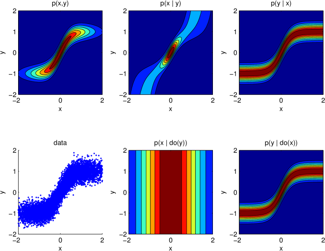
Figure 4: Identifiable ANM with $Y=\tanh(X)+E$, where $X\sim\mathcal{N}(0,1)$ and $E\sim\mathcal{N}(0,0.5^{2})$. Shown are contours of the joint and conditional distributions, and a scatter plot of data sampled from the model distribution. Note that the contour lines of $p(y\,|\,x)$ only shift as $x$ changes. On the other hand, $p(x\,|\,y)$ differs by more than just its mean for different values of $y$.

Hoyer et al. (2009) proved that additive noise models are generically identifiable. The intuition behind this result is that if $p(x,y)$ satisfies an additive noise model $X\to Y$, then $p(y\,|\,x)$ depends on $x$ only through its mean, and all other aspects of this conditional distribution do not depend on $x$. On the other hand, $p(x\,|\,y)$ will typically depend in a more complicated way on $y$ (see also Figure 4). Only for very specific choices of the parameters of an ANM one obtains a non-identifiable ANM. We have already seen an example of such a non-identifiable ANM: the linear-Gaussian case (Example 1). A more exotic example with non-Gaussian distributions was given in (Peters et al., 2014, Example 25). Zhang and Hyvärinen (2009) proved that non-identifiable ANMs necessarily fall into one out of five classes. In particular, their result implies something that we might expect intuitively: if $f$ is not injective, the ANM is identifiable.

Mooij et al. (2011) showed that bivariate identifiability even holds generically when feedback is allowed (i.e., if both $X\rightarrow Y$ and $Y\rightarrow X$), at least when assuming noise and input distributions to be Gaussian. Peters et al. (2011) provide an extension of the acyclic model for discrete variables. Zhang and Hyvärinen (2009) give an extension of the identifiability results allowing for an additional bijective transformation of the data, i.e., using a functional model of the form $Y=\phi\big{(}f_{Y}(X)+E_{Y}\big{)}$, with $E_{Y}\mbox{${}\perp\mkern-11.0mu\perp{}$}X$, and $\phi:\mathbb{R}\to\mathbb{R}$ bijective, which they call the Post-NonLinear (PNL) model. The results on identifiability of additive noise models can be extended to the multivariate case (Peters et al., 2014) if there are no hidden variables and no feedback loops. This extension can be applied to nonlinear ANMs (Hoyer et al., 2009; Bühlmann et al., 2014), linear non-Gaussian models (Shimizu et al., 2011), the model of equal error variances (Peters and Bühlmann, 2014) or to the case of discrete variables (Peters et al., 2011). Full identifiability in the presence of hidden variables for the acyclic case has only been established for linear non-Gaussian models (Hoyer et al., 2008).

2.1.3 Additive Noise Principle

Following Hoyer et al. (2009), we hypothesize that:

Principle 1

Suppose we are given a joint density $p(x,y)$ and we know that the causal structure is either that of (a) or (b) in Figure 2. If $p(x,y)$ satisfies an identifiable additive noise model $X\to Y$, then it is likely that we are in case (a), i.e., $X$ causes $Y$.

This principle should not be regarded as a rigorous statement, but rather as an empirical assumption: we cannot exactly quantify how likely the conclusion that $X$ causes $Y$ is, as there is always a possibility that $Y$ causes $X$ while $p_{X,Y}$ happens to satisfy an identifiable additive noise model $X\to Y$. In general, that would require a special choice of the distribution of $X$ and the conditional distribution of $Y$ given $X$, which is unlikely. In this sence, we can regard this principle as a special case of Occam’s Razor.

In the next subsection, we will discuss various ways of operationalizing this principle. In Section 4, we provide empirical evidence supporting this principle.

2.2 Estimation methods

The following Lemma is helpful to test whether a density satisfies a bivariate additive noise model:

Lemma 7

Given a joint density $p(x,y)$ of two random variables $X,Y$ such that the conditional expectation $\mathbb{E}(Y\,|\,X=x)$ is well-defined for all $x$ and measurable. Then, $p(x,y)$ satisfies a bivariate additive noise model $X\to Y$ if and only if $E_{Y}:=Y-\mathbb{E}(Y\,|\,X)$ has finite mean and is independent of $X$.

Proof  Suppose that $p(x,y)$ is induced by $(p_{X},p_{U},f)$, say $Y=f(X)+U$ with $X\mbox{${}\perp\mkern-11.0mu\perp{}$}U$, $X\sim p_{X}$, $U\sim p_{U}$. Then $\mathbb{E}(Y\,|\,X=x)=f(x)+\nu$, with $\nu=\mathbb{E}(U)$. Therefore, $E_{Y}=Y-\mathbb{E}(Y\,|\,X)=Y-(f(X)+\nu)=U-\nu$ is independent of $X$. Conversely, if $E_{Y}$ is independent of $X$, $p(x,y)$ is induced by the bivariate additive noise model $(p_{X},p_{E_{Y}},x\mapsto\mathbb{E}(Y\,|\,X=x))$.  
In practice, we usually do not have the density $p(x,y)$, but rather a finite sample of it. In that case, we can use the same idea for testing whether this sample comes from a density that satisfies an additive noise model: we estimate the conditional expectation $\mathbb{E}(Y\,|\,X)$ by regression, and then test the independence of the residuals $Y-\mathbb{E}(Y\,|\,X)$ and $X$.

Suppose we have two data sets, a training data set $\mathcal{D}_{N}:=\{(x_{n},y_{n})\}_{n=1}^{N}$ (for estimating the function) and a test data set $\mathcal{D}_{N}^{\prime}:=\{(x_{n}^{\prime},y_{n}^{\prime})\}_{n=1}^{N}$ (for testing independence of residuals), both consisting of i.i.d. samples distributed according to $p(x,y)$. We will write $\bm{x}=(x_{1},\dots,x_{N})$, $\bm{y}=(y_{1},\dots,y_{N})$, $\bm{x}^{\prime}=(x_{1}^{\prime},\dots,x_{N}^{\prime})$ and $\bm{y}^{\prime}=(y_{1}^{\prime},\dots,y_{N}^{\prime})$. We will consider two scenarios: the “data splitting” scenario where training and test set are independent (typically achieved by splitting a bigger data set into two parts), and the “data recycling” scenario in which the training and test data are identical (where we use the same data twice for different purposes: regression and independence testing).

Hoyer et al. (2009) suggested the following procedure to test whether the data come from a density that satisfies an additive noise model. By regressing $Y$ on $X$ using the training data $\mathcal{D}_{N}$, an estimate $\hat{f}_{Y}$ for the regression function $x\mapsto\mathbb{E}(Y\,|\,X=x)$ is obtained. Then, an independence test is used to estimate whether the predicted residuals are independent of the input, i.e., whether $(Y-\hat{f}_{Y}(X))\mbox{${}\perp\mkern-11.0mu\perp{}$}X$, using test data $(\bm{x}^{\prime},\bm{y}^{\prime})$. If the null hypothesis of independence is not rejected, one concludes that $p(x,y)$ satisfies an additive noise model $X\to Y$. The regression procedure and the independence test can be freely chosen.

There is a caveat, however: under the null hypothesis that $p(x,y)$ indeed satisfies an ANM, the error in the estimated residuals may introduce a dependence between the predicted residuals $\bm{\hat{e}}_{Y}^{\prime}:=\bm{y}^{\prime}-\hat{f}_{Y}(\bm{x}^{\prime})$ and $\bm{x}^{\prime}$ even if the true residuals $\bm{y}^{\prime}-\mathbb{E}(Y\,|\,X=\bm{x}^{\prime})$ are independent of $\bm{x}^{\prime}$. Therefore, the threshold for the independence test statistic has to be chosen with care: the standard threshold that would ensure consistency of the independence test on its own may be too tight. As far as we know, there are no theoretical results on the choice of that threshold that would lead to a consistent way to test whether $p(x,y)$ satisfies an ANM $X\to Y$.

We circumvent this problem by assuming a priori that $p(x,y)$ either satisfies an ANM $X\to Y$, or an ANM $Y\to X$, but not both. In that sense, the test statistics of the independence test can be directly compared, and no threshold needs to be chosen. This leads us to Algorithm 1 as a general scheme for identifying the direction of the ANM. In order to decide whether $p(x,y)$ satisfies an additive noise model $X\to Y$, or an additive noise model $Y\to X$, we simply estimate the regression functions in both directions, calculate the corresponding residuals, estimate the dependence of the residuals with respect to the input by some dependence measure $\hat{C}$, and output the direction that has the lowest dependence.

Algorithm 1 General procedure to decide whether $p(x,y)$ satisfies an additive noise model $X\to Y$ or $Y\to X$.

Input:

1. I.i.d. sample $\mathcal{D}_{N}:=\{(x_{i},y_{i})\}_{i=1}^{N}$ of $X$ and $Y$ (“training data”);

2. I.i.d. sample $\mathcal{D}_{N}^{\prime}:=\{(x_{i}^{\prime},y_{i}^{\prime})\}_{i=1}^{N}$ of $X$ and $Y$ (“test data”);

3. Regression method;

4. Score estimator $\hat{C}:\mathbb{R}^{N}\times\mathbb{R}^{N}\to\mathbb{R}$.

Output: $\hat{C}_{X\to Y}$, $\hat{C}_{Y\to X}$, dir.

1. Use the regression method to obtain estimates:

   1. $\hat{f}_{Y}$ of the regression function $x\mapsto\mathbb{E}(Y\,|\,X=x)$,

   2. $\hat{f}_{X}$ of the regression function $y\mapsto\mathbb{E}(X\,|\,Y=y)$

   using the training data $\mathcal{D}_{N}$;

2. Use the estimated regression functions to predict residuals:

   1. $\bm{\hat{e}}_{Y}^{\prime}:=\bm{y}^{\prime}-\hat{f}_{Y}(\bm{x}^{\prime})$

   2. $\bm{\hat{e}}_{X}^{\prime}:=\bm{x}^{\prime}-\hat{f}_{X}(\bm{y}^{\prime})$

   from the test data $\mathcal{D}_{N}^{\prime}$.

3. Calculate the scores to measure dependence of inputs and estimated residuals on the test data $\mathcal{D}_{N}^{\prime}$:

   1. $\hat{C}_{X\to Y}:=\hat{C}(\bm{x}^{\prime},\bm{\hat{e}}_{Y}^{\prime})$;

   2. $\hat{C}_{Y\to X}:=\hat{C}(\bm{y}^{\prime},\bm{\hat{e}}_{X}^{\prime})$;

4. Output $\hat{C}_{X\to Y},\hat{C}_{Y\to X}$ and:

   $$\mathtt{dir}:=\begin{cases}X\to Y&\text{ if }\hat{C}_{X\to Y}<\hat{C}_{Y\to X},\\ Y\to X&\text{ if }\hat{C}_{X\to Y}>\hat{C}_{Y\to X},\\ ?&\text{ if }\hat{C}_{X\to Y}=\hat{C}_{Y\to X}.\end{cases}$$

In principle, any consistent regression method can be used in Algorithm 1. Likewise, in principle any consistent measure of dependence can be used in Algorithm 1 as score function. In the next subsections, we will consider in more detail some possible choices for the score function. Originally, Hoyer et al. (2009) proposed to use the $p$-value of the Hilbert Schmidt Independence Criterion (HSIC), a kernel-based non-parametric independence test. Alternatively, one can also use the HSIC statistic itself as a score, and we will show that this leads to a consistent procedure. Other dependence measures could be used instead, e.g., the measure proposed by Reshef et al. (2011). Kpotufe et al. (2014); Nowzohour and Bühlmann (2015) proposed to use as a score the sum of the estimated differential entropies of inputs and residuals and proved consistency of that procedure. For the Gaussian case, that is equivalent to the score considered in a high-dimensional context that was shown to be consistent by Bühlmann et al. (2014). This Gaussian score is also strongly related to an empirical-Bayes score originally proposed by Friedman and Nachman (2000). Finally, we will briefly discuss a Minimum Message Length score that was considered by Mooij et al. (2010) and another idea (based on minimizing a dependence measure directly) proposed by Mooij et al. (2009).

2.2.1 HSIC-based scores

One possibility, first considered by Hoyer et al. (2009), is to use the Hilbert-Schmidt Independence Criterion (HSIC) (Gretton et al., 2005) for testing the independence of the estimated residuals with the inputs. See Appendix A.1 for a definition and basic properties of the HSIC independence test.

As proposed by Hoyer et al. (2009), one can use the $p$-value of the HSIC statistic under the null hypothesis of independence. This amounts to the following score function for measuring dependence:

$$\hat{C}(\bm{u},\bm{v}):=-\log\hat{p}_{\mathrm{HSIC}_{\kappa_{\hat{\ell}(\bm{u})},\kappa_{\hat{\ell}(\bm{v})}}}(\bm{u},\bm{v}).$$ (5)

Here, $\kappa_{\ell}$ is a kernel with parameters $\ell$, that are estimated from the data. $\bm{u}$ and $\bm{v}$ are either inputs or estimated residuals (see also Algorithm 1). A low HSIC $p$-value indicates that we should reject the null hypothesis of independence. Another possibility is to use the HSIC value itself (instead of its $p$-value):

$$\hat{C}(\bm{u},\bm{v}):=\widehat{\mathrm{HSIC}}{\kappa_{\hat{\ell}(\bm{u})},\kappa_{\hat{\ell}(\bm{v})}}(\bm{u},\bm{v}).$$ (6)

An even simpler option is to use a fixed kernel $k$:

$$\hat{C}(\bm{u},\bm{v}):=\widehat{\mathrm{HSIC}}_{k,k}(\bm{u},\bm{v}).$$ (7)

In Appendix A, we prove that under certain technical assumptions, Algorithm 1 with score function (7) is a consistent procedure for inferring the direction of the ANM. In particular, the product kernel $k\cdot k$ should be characteristic in order for HSIC to detect all possible independencies, and the regression method should satisfy the following condition:

Definition 8

Let $X,Y$ be two real-valued random variables with joint distribution $\mathbb{P}_{X,Y}$. Suppose we are given sequences of training data sets $\mathcal{D}_{N}=\{X_{1},X_{2},\dots,X_{N}\}$ and test data sets $\mathcal{D}_{N}^{\prime}=\{X_{1}^{\prime},X_{2}^{\prime},\dots,X_{N}^{\prime}\}$ (in either the data splitting or the data recycling scenario). We call a regression method suitable for regressing $Y$ on $X$ if the mean squared error between true and estimated regression function, evaluated on the test data, vanishes asymptotically in expectation:

$$\lim_{N\to\infty}\mathbb{E}_{\mathcal{D}_{N},\mathcal{D}_{N}^{\prime}}\left(\frac{1}{N}\sum_{n=1}^{N}\left|\hat{f}_{Y}(X_{n}^{\prime};\mathcal{D}_{N})-\mathbb{E}(Y\,|\,X=X_{n}^{\prime})\right|^{2}\right)=0.$$ (8)

Here, the expectation is taken over both training data $\mathcal{D}_{N}$ and test data $\mathcal{D}_{N}^{\prime}$.

The consistency result then reads as follows:

Theorem 9

Let $X,Y$ be two real-valued random variables with joint distribution $\mathbb{P}_{X,Y}$ that either satisfies an additive noise model $X\to Y$, or $Y\to X$, but not both. Suppose we are given sequences of training data sets $\mathcal{D}_{N}$ and test data sets $\mathcal{D}_{N}^{\prime}$ (in either the data splitting or the data recycling scenario). Let $k:\mathbb{R}\times\mathbb{R}\to\mathbb{R}$ be a bounded non-negative Lipschitz-continuous kernel such that the product $k\cdot k$ is characteristic. If the regression procedure used in Algorithm 1 is suitable for both $\mathbb{P}_{X,Y}$ and $\mathbb{P}_{Y,X}$, then Algorithm 1 with score (7) is a consistent procedure for estimating the direction of the additive noise model.

Proof  See Appendix A (where a slightly more general result is shown, allowing for two different kernels $k,l$ to be used). The main technical difficulty consists of the fact that the error in the estimated regression function introduces a dependency between the cause and the estimated residuals. We overcome this difficulty by showing that the dependence is so weak that its influence on the test statistic vanishes asymptotically.  
In the data splitting case, weakly universally consistent regression methods (Györfi et al., 2002) are suitable. In the data recycling scenario, any regression method that satisfies (8) is suitable. An example of a kernel $k$ that satisfies the conditions of Theorem 9 is the Gaussian kernel.

2.2.2 Entropy-based scores

Instead of explicitly testing for independence of residuals and inputs, one can use the sum of their differential entropies as a score function (e.g., Kpotufe et al., 2014; Nowzohour and Bühlmann, 2015). This can easily be seen using Lemma 1 of Kpotufe et al. (2014), which we reproduce here because it is very instructive:

Lemma 10

Consider a joint distribution of $X,Y$ with density $p(x,y)$. For arbitrary functions $f,g:\mathbb{R}\to\mathbb{R}$ we have:

$$H(X)+H(Y-f(X))=H(Y)+H(X-g(Y))-\big{(}I(X-g(Y),Y)-I(Y-f(X),X)\big{)}.$$

where $H(\cdot)$ denotes differential Shannon entropy, and $I(\cdot,\cdot)$ denotes differential mutual information (Cover and Thomas, 2006).  

The proof is a simple application of the chain rule of differential entropy. If $p(x,y)$ satisfies an identifiable additive noise model $X\to Y$, then there exists a function $f$ with $I(Y-f(X),X)=0$ (e.g., the regression function $x\mapsto\mathbb{E}(Y\,|\,X=x)$), but $I(X-g(Y),Y)>0$ for any function $g$. Therefore, one can use Algorithm 1 with score function

$$\hat{C}(\bm{u},\bm{v}):=\hat{H}(\bm{u})+\hat{H}(\bm{v})$$ (9)

in order to estimate the causal direction, using any estimator $\hat{H}(\cdot)$ of the differential Shannon entropy. Kpotufe et al. (2014); Nowzohour and Bühlmann (2015) prove that this approach to estimating the direction of additive noise models is consistent under certain technical assumptions.

Kpotufe et al. (2014) note that the advantage of score (9) (based on marginal entropies) over score (6) (based on dependence) is that marginal entropies are cheaper to estimate than dependence (or mutual information). This is certainly true when considering computation time. However, as we will see later, a disadvantage of relying on differential entropy estimators is that these can be quite sensitive to discretization effects.

2.2.3 Gaussian score

The differential entropy of a random variable $X$ can be upper bounded in terms of its variance (see e.g., Cover and Thomas, 2006, Theorem 8.6.6):

$$H(X)\leq\frac{1}{2}\log(2\pi e)+\frac{1}{2}\log\mathbb{V}\mathrm{ar}(X),$$ (10)

where identity holds in case $X$ has a Gaussian distribution. Assuming that $p(x,y)$ satisfies an identifiable Gaussian additive noise model $X\to Y$ with Gaussian input and Gaussian noise distributions, we therefore conclude from Lemma 10:

$$\begin{split}\log\mathbb{V}\mathrm{ar}(X)+\log\mathbb{V}\mathrm{ar}(Y-\hat{f}(X))&=2H(X)+2H(Y-\hat{f}(X))-2\log(2\pi e)\\ &<2H(Y)+2H(X-\hat{g}(Y))-2\log(2\pi e)\\ &\leq\log\mathbb{V}\mathrm{ar}Y+\log\mathbb{V}\mathrm{ar}(X-\hat{g}(Y))\end{split}$$

for any function $g$. In that case, we can therefore use Algorithm 1 with score function

$$\hat{C}(\bm{u},\bm{v}):=\log\widehat{\mathbb{V}\mathrm{ar}}(\bm{u})+\log\widehat{\mathbb{V}\mathrm{ar}}(\bm{v}).$$ (11)

This score was also considered recently by Bühlmann et al. (2014) and shown to lead to a consistent estimation procedure under certain assumptions.

2.2.4 Empirical-Bayes scores

Deciding the direction of the ANM can also be done by applying model selection using empirical Bayes. As an example, for the ANM $X\to Y$, one can consider a generative model that models $X$ as a Gaussian, and $Y$ as a Gaussian Process (Rasmussen and Williams, 2006) conditional on $X$. For the ANM $Y\to X$, one considers a similar model with the roles of $X$ and $Y$ reversed. Empirical-Bayes model selection is performed by calculating the maximum evidences (marginal likelihoods) of these two models when optimizing over the hyperparameters, and preferring the model with larger maximum evidence. This is actually a special case (the bivariate case) of an approach proposed by Friedman and Nachman (2000). Considering the negative log marginal likelihoods leads to the following score for the ANM $X\to Y$:

$$\hat{C}_{X\to Y}(\bm{x},\bm{y}):=\min_{\mu,\tau^{2},\bm{\theta},\sigma^{2}}\left(-\log\mathcal{N}(\bm{x}\,|\,\mu\bm{1},\tau^{2}\bm{I})-\log\mathcal{N}(\bm{y}\,|\,\bm{0},\bm{K}_{\bm{\theta}}(\bm{x})+\sigma^{2}\bm{I})\right),$$ (12)

and a similar expression for $\hat{C}_{Y\to X}$, the score of the ANM $Y\to X$. Here, $\bm{K}_{\bm{\theta}}(\bm{x})$ is the $N\times N$ kernel matrix $K_{ij}=k_{\bm{\theta}}(x_{i},x_{j})$ for a kernel with parameters $\bm{\theta}$ and $\mathcal{N}(\cdot\,|\,\bm{\mu},\bm{\Sigma})$ denotes the density of a multivariate normal distribution with mean $\bm{\mu}$ and covariance matrix $\bm{\Sigma}$. If one would put a prior distribution on the hyperparameters and integrate them out, this would correspond to Bayesian model selection. In practice, one typically uses “empirical Bayes”, which means that the hyperparameters $(\mu,\tau,\bm{\theta},\sigma)$ are optimized over instead for computational reasons. Note that this method skips the explicit regression step, instead it (implicitly) integrates over all possible regression functions (Rasmussen and Williams, 2006). Also, it does not distinguish the data splitting and data recycling scenarios, instead it uses the data directly to calculate the (maximum) marginal likelihood. Therefore, the structure of the algorithm is slightly different, see Algorithm 2. In Appendix B we show that this score is actually closely related to the Gaussian score considered in Section 2.2.3.

Algorithm 2 Procedure to decide whether $p(x,y)$ satisfies an additive noise model $X\to Y$ or $Y\to X$ suitable for empirical-Bayes or MML model selection.

Input:

1. I.i.d. sample $\mathcal{D}_{N}:=\{(x_{i},y_{i})\}_{i=1}^{N}$ of $X$ and $Y$ (“data”);

2. Score function $\hat{C}:\mathbb{R}^{N}\times\mathbb{R}^{N}\to\mathbb{R}$ for measuring model fit and model complexity.

Output: $\hat{C}_{X\to Y}$, $\hat{C}_{Y\to X}$, dir.

1. 1. calculate $\hat{C}_{X\to Y}=\hat{C}(\bm{x},\bm{y})$

   2. calculate $\hat{C}_{Y\to X}=\hat{C}(\bm{y},\bm{x})$

2. Output $\hat{C}_{X\to Y},\hat{C}_{Y\to X}$ and:

   $$\mathtt{dir}:=\begin{cases}X\to Y&\text{ if }\hat{C}_{X\to Y}<\hat{C}_{Y\to X},\\ Y\to X&\text{ if }\hat{C}_{X\to Y}>\hat{C}_{Y\to X},\\ ?&\text{ if }\hat{C}_{X\to Y}=\hat{C}_{Y\to X}.\end{cases}$$

2.2.5 Minimum Message Length scores

In a similar vein as (empirical) Bayesian marginal likelihoods can be interpreted as measuring likelihood in combination with a complexity penalty, Minimum Message Length (MML) techniques can be used to construct scores that incorporate a trade-off between model fit (likelihood) and model complexity (Grünwald, 2007). Asymptotically, as the number of data points tends to infinity, one would expect the model fit to outweigh the model complexity, and therefore by Lemma 10, simple comparison of MML scores should be enough to identify the direction of an identifiable additive noise model.

A particular MML score was considered by Mooij et al. (2010). This is a special case (referred to in Mooij et al. (2010) as “AN-MML”) of their more general framework that allows for non-additive noise. Like (12), the score is a sum of two terms, one corresponding to the marginal density $p(x)$ and the other to the conditional density $p(y\,|\,x)$:

$$\hat{C}_{X\to Y}(\bm{x},\bm{y}):=\mathcal{L}(\bm{x})+\min_{\bm{\theta},\sigma^{2}}\left(-\log\mathcal{N}(\bm{y}\,|\,0,\bm{K}_{\theta}(\bm{x})+\sigma^{2}\bm{I})\right).$$ (13)

The second term is an MML score for the conditional density $p(y\,|\,x)$, and is identical to the conditional density term in (12). The MML score $\mathcal{L}(\bm{x})$ for the marginal density $p(x)$ is derived as an asymptotic expansion based on the Minimum Message Length principle for a mixture-of-Gaussians model (Figueiredo and Jain, 2002):

$$\mathcal{L}(\bm{x})=\min_{\bm{\eta}}\left(\sum_{j=1}^{k}\log\left(\frac{N\alpha_{j}}{12}\right)+\frac{k}{2}\log\frac{N}{12}+\frac{3k}{2}-\log p(\bm{x}\,|\,\bm{\eta})\right),$$ (14)

where $p(\bm{x}\,|\,\bm{\eta})$ is a Gaussian mixture model: $p(x_{i}\,|\,\bm{\eta})=\sum_{j=1}^{k}\alpha_{j}\mathcal{N}(x_{i}\,|\,\mu_{j},\sigma_{j}^{2})$ with $\bm{\eta}=(\alpha_{i},\mu_{i},\sigma^{2}_{i})_{i=1}^{k}$. The optimization problem (14) is solved numerically by means of the algorithm proposed by Figueiredo and Jain (2002), using a small but nonzero value ($10^{-4}$) of the regularization parameter.

Comparing this score with the empirical-Bayes score (12), the main conceptual difference is that the former uses a more complicated mixture-of-Gaussians model for the marginal density, whereas (12) uses a simple Gaussian model. We can use (13) in combination with Algorithm 2 in order to estimate the direction of an identifiable additive noise model.

2.2.6 Minimizing HSIC directly

One can try to apply the idea of combining regression and independence testing into a single procedure (as achieved with the empirical-Bayes score described in Section 2.2.4, for example) more generally. Indeed, a score that measures the dependence between the residuals $\bm{y}^{\prime}-f_{Y}(\bm{x}^{\prime})$ and the inputs $\bm{x}^{\prime}$ can be minimized with respect to the function $f_{Y}$. Mooij et al. (2009) proposed to minimize $\widehat{\mathrm{HSIC}}\big{(}\bm{x},\bm{y}-f(\bm{x})\big{)}$ with respect to the function $f$. However, the optimization problem with respect to $f$ turns out to be a challenging non-convex optimization problem with multiple local minima, and there are no guarantees to find the global minimum. In addition, the performance depends strongly on the selection of suitable kernel bandwidths, for which no suitable automatic procedure is known in this context. Finally, proving consistency of such a method might be challenging, as the minimization may introduce strong dependences between the residuals. Therefore, we do not discuss or evaluate this method in more detail here.

3 Information-Geometric Causal Inference

In this section, we review a class of causal discovery methods that exploits independence of the distribution of the cause and the conditional distribution of the effect given the cause. It nicely complements causal inference based on additive noise by employing asymmetries between cause and effect that have nothing to do with noise.

3.1 Theory

Information-Geometric Causal Inference (IGCI) is an approach that builds upon the assumption that for $X\rightarrow Y$ the marginal distribution $\mathbb{P}_{X}$ contains no information about the conditional $\mathbb{P}_{Y\,|\,X}$ and vice versa, since they represent independent mechanisms. As Janzing and Schölkopf (2010) illustrated for several toy examples, the conditional and marginal distributions $\mathbb{P}_{Y},\mathbb{P}_{X\,|\,Y}$ may then contain information about each other, but it is hard to formalize in what sense this is the case for scenarios that go beyond simple toy models. IGCI is based on the strong assumption that $X$ and $Y$ are deterministically related by a bijective function $f$, that is, $Y=f(X)$ and $X=f^{-1}(Y)$. Although its practical applicability is limited to causal relations with sufficiently small noise and sufficiently high non-linearity, IGCI provides a setting in which the independence of $\mathbb{P}_{X}$ and $\mathbb{P}_{Y\,|\,X}$ provably implies well-defined dependences between $\mathbb{P}_{Y}$ and $\mathbb{P}_{X\,|\,Y}$ in a sense described below.

To introduce IGCI, note that the deterministic relation $Y=f(X)$ implies that the conditional $\mathbb{P}_{Y\,|\,X}$ has no density $p(y\,|\,x)$, but it can be represented using $f$ via

$$\mathbb{P}(Y=y\,|\,X=x)=\left\{\begin{array}[]{cc}1&\hbox{ if }y=f(x)\\ 0&\hbox{ otherwise. }\end{array}\right.$$

The fact that $\mathbb{P}_{X}$ and $\mathbb{P}_{Y\,|\,X}$ contain no information about each other then translates into the statement that $\mathbb{P}_{X}$ and $f$ contain no information about each other.

Before sketching a more general formulation of IGCI (Daniušis et al., 2010; Janzing et al., 2012), we begin with the most intuitive case where $f$ is a strictly monotonically increasing differentiable bijection of $[0,1]$. We then assume that the following equality is approximately satisfied:

$$\int_{0}^{1}\log f^{\prime}(x)p(x)\,dx=\int_{0}^{1}\log f^{\prime}(x)\,dx,$$ (15)

where $f^{\prime}$ is the derivative of $f$. To see why (15) is an independence between function $f$ and input density $p_{X}$, we interpret $x\mapsto\log f^{\prime}(x)$ and $x\mapsto p(x)$ as random variables on the probability space $[0,1]$. Then the difference between the two sides of (15) is the covariance of these two random variables with respect to the uniform distribution on $[0,1]$:

$$\begin{split}\mathbb{C}\mathrm{ov}(\log f^{\prime},p_{X})&=\mathbb{E}(\log f^{\prime}\cdot p_{X})-\mathbb{E}(\log f^{\prime})\mathbb{E}(p_{X})\\ &=\int\log f^{\prime}(x)\cdot p(x)dx-\int\log f^{\prime}(x)dx\int p(x)dx\,.\end{split}$$

As shown in Section 2 in (Daniušis et al., 2010), $p_{Y}$ is then related to the inverse function $f^{-1}$ in the sense that

$$\int_{0}^{1}\log(f^{-1})^{\prime}(y)\cdot p(y)\,dy\geq\int_{0}^{1}\log(f^{-1})^{\prime}(y)\,dy\,,$$

with equality if and only if $f^{\prime}$ is constant. Hence, $\log(f^{-1})^{\prime}$ and $p_{Y}$ are positively correlated due to

$$\mathbb{E}\big{(}\log(f^{-1})^{\prime}\cdot p_{Y}\big{)}-\mathbb{E}\big{(}\log(f^{-1})^{\prime}\big{)}\mathbb{E}(p_{Y})>0\,.$$

Intuitively, this is because the density $p_{Y}$ tends to be high in regions where $f$ is flat, or equivalently, $f^{-1}$ is steep (see also Figure 5). Hence, we have shown that $\mathbb{P}_{Y}$ contains information about $f^{-1}$ and hence about $\mathbb{P}_{X\,|\,Y}$ whenever $\mathbb{P}_{X}$ does not contain information about $\mathbb{P}_{Y\,|\,X}$ (in the sense that (15) is satisfied), except for the trivial case where $f$ is linear.

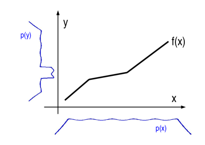
Figure 5: Illustration of the basic intuition behind IGCI. If the density $p_{X}$ of the cause $X$ is not correlated with the slope of $f$, then the density $p_{Y}$ tends to be high in regions where $f$ is flat (and $f^{-1}$ is steep). Source: Janzing et al. (2012).

To employ this asymmetry, Daniušis et al. (2010) introduce the expressions

$$C_{X\to Y} := \int_{0}^{1}\log f^{\prime}(x)p(x)dx$$ (16)

$$C_{Y\to X} := \int_{0}^{1}\log(f^{-1})^{\prime}(y)p(y)dy=-C_{X\to Y}\,.$$ (17)

Since the right hand side of (15) is smaller than zero due to $\int_{0}^{1}\log f^{\prime}(x)dx\leq\log\int_{0}^{1}f^{\prime}(x)dx=0$ by concavity of the logarithm (exactly zero only for constant $f$), IGCI infers $X\to Y$ whenever $C_{X\to Y}$ is negative. Section 3.5 in (Daniušis et al., 2010) also shows that

$$C_{X\to Y}=H(Y)-H(X)\,,$$

i.e., the decision rule considers the variable with lower differential entropy as the effect. The idea is that the function introduces new irregularities to a distribution rather than smoothing the irregularities of the distribution of the cause.

Generalization to other reference measures: In the above version of IGCI the uniform distribution on $[0,1]$ plays a special role because it is the distribution with respect to which uncorrelatedness between $p_{X}$ and $\log f^{\prime}$ is defined. The idea can be generalized to other reference distributions. How to choose the right one for a particular inference problem is a difficult question which goes beyond the scope of this article. From a high-level perspective, it is comparable to the question of choosing the right kernel for kernel-based machine learning algorithms; it also is an a priori structure of the range of $X$ and $Y$ without which the inference problem is not well-defined.

Let $u_{X}$ and $u_{Y}$ be densities of $X$ and $Y$, respectively, that we call “reference densities”. For example, uniform or Gaussian distributions would be reasonable choices. Let $u_{f}$ be the image of $u_{X}$ under $f$ and $u_{f^{-1}}$ be the image of $u_{Y}$ under $f^{-1}$. Then we hypothesize the following generalization of (15):

Principle 2

If $X$ causes $Y$ via a deterministic bijective function $f$ such that $u_{f^{-1}}$ has a density with respect to Lebesgue measure, then

$$\int\log\frac{u_{f^{-1}}(x)}{u_{X}(x)}p(x)\,dx\approx\int\log\frac{u_{f^{-1}}(x)}{u_{X}(x)}u_{X}(x)\,dx\,.$$ (18)

In analogy to the remarks above, this can also be interpreted as uncorrelatedness of the functions $\log(u_{f^{-1}}/u_{X})$ and $p_{X}/u_{X}$ with respect to the measure given by the density of $u_{X}$ with respect to the Lebesgue measure. Again, we hypothesize this because the former expression is a property of the function $f$ alone (and the reference densities) and should thus be unrelated to the marginal density $p_{X}$. The special case (15) can be obtained by taking the uniform distribution on $[0,1]$ for $u_{X}$ and $u_{Y}$.

As generalization of (16,17) we define

$$C_{X\to Y} := \int\log\frac{u_{f^{-1}}(x)}{u_{X}(x)}p(x)dx$$ (19)

$$C_{Y\to X} := \int\log\frac{u_{f}(y)}{u_{Y}(y)}p(y)dy=\int\log\frac{u_{X}(x)}{u_{f^{-1}}(x)}p(x)dx=-C_{Y\to X}\,,$$ (20)

where the second equality in (20) follows by substitution of variables. Again, the hypothesized independence implies $C_{X\to Y}\leq 0$ since the right hand side of (18) coincides with $-D(u_{X}\|u_{f^{-1}})$ where $D(\cdot\|\cdot)$ denotes Kullback-Leibler divergence. Hence, we also infer $X\to Y$ whenever $C_{X\to Y}<0$. Note also that

$$C_{X\to Y}=D(p_{X}\|u_{X})-D(p_{X}\|u_{f^{-1}})=D(p_{X}\|u_{X})-D(p_{Y}\|u_{Y})\,,$$

where we have only used the fact that relative entropy is preserved under bijections. Hence, our decision rule amounts to inferring that the density of the cause is closer to its reference density. This decision rule gets quite simple, for instance, if $u_{X}$ and $u_{Y}$ are Gaussians with the same mean and variance as $p_{X}$ and $p_{Y}$, respectively. Then it again amounts to inferring $X\rightarrow Y$ whenever $X$ has larger entropy than $Y$ after rescaling both $X$ and $Y$ to have the same variance.

3.2 Estimation methods

The specification of the reference measure is essential for IGCI. We describe the implementation for two different choices:

1. Uniform distribution: scale and shift $X$ and $Y$ such that extrema are mapped onto $0$ and $1$.

2. Gaussian distribution: scale $X$ and $Y$ to variance 1.

Given this preprocessing step, there are different options for estimating $C_{X\to Y}$ and $C_{Y\to X}$ from empirical data (see Section 3.5 in (Daniušis et al., 2010)):

1. Slope-based estimator:

   $$\hat{C}_{X\rightarrow Y}:=\frac{1}{N-1}\sum_{j=1}^{N-1}\log\frac{|y_{j+1}-y_{j}|}{x_{j+1}-x_{j}}\,,$$ (21)

   where we assumed the pairs $\{(x_{i},y_{i})\}$ to be ordered ascendingly according to $x_{i}$. Since empirical data are noisy, the $y$-values need not be in the same order. $\hat{C}_{Y\to X}$ is given by exchanging the roles of $X$ and $Y$.

2. Entropy-based estimator:

   $$\hat{C}_{X\to Y}:=\hat{H}(Y)-\hat{H}(X)\,,$$ (22)

   where $\hat{H}(\cdot)$ denotes some differential entropy estimator.

The theoretical equivalence between these estimators breaks down on empirical data not only due to finite sample effects but also because of noise. For the slope based estimator, we even have

$$\hat{C}_{X\to Y}\neq-\hat{C}_{Y\to X}\,,$$

and thus need to compute both terms separately.

Algorithm 3 General procedure to decide whether $\mathbb{P}_{X,Y}$ is generated by a deterministic monotonic bijective function from $X$ to $Y$ or from $Y$ to $X$.

Input:

1. I.i.d. sample $\mathcal{D}_{N}:=\{(x_{i},y_{i})\}_{i=1}^{N}$ of $X$ and $Y$ (“data”);

2. Normalization procedure $\nu:\mathbb{R}^{N}\to\mathbb{R}^{N}$;

3. IGCI score estimator $\hat{C}:\mathbb{R}^{N}\times\mathbb{R}^{N}\to\mathbb{R}$.

Output: $\hat{C}_{X\to Y}$, $\hat{C}_{Y\to X}$, dir.

1. Normalization:

   1. calculate $\tilde{\bm{x}}=\nu(\bm{x})$

   2. calculate $\tilde{\bm{y}}=\nu(\bm{y})$

2. Estimation of scores:

   1. calculate $\hat{C}_{X\to Y}=\hat{C}(\tilde{\bm{x}},\tilde{\bm{y}})$

   2. calculate $\hat{C}_{Y\to X}=\hat{C}(\tilde{\bm{y}},\tilde{\bm{x}})$

3. Output $\hat{C}_{X\to Y},\hat{C}_{Y\to X}$ and:

   $$\mathtt{dir}:=\begin{cases}X\to Y&\text{ if }\hat{C}_{X\to Y}<\hat{C}_{Y\to X},\\ Y\to X&\text{ if }\hat{C}_{X\to Y}>\hat{C}_{Y\to X},\\ ?&\text{ if }\hat{C}_{X\to Y}=\hat{C}_{Y\to X}.\end{cases}$$

Note that the IGCI implementations discussed here make sense only for continuous variables with a density with respect to Lebesgue measure. This is because the difference quotients are undefined if a value occurs twice. In many empirical data sets, however, the discretization (e.g., due to rounding to some number of digits) is not fine enough to guarantee this. A very preliminary heuristic that was employed in earlier work (Daniušis et al., 2010) removes repeated occurrences by removing data points, but a conceptually cleaner solution would be, for instance, the following procedure: Let ${\tilde{x}}_{j}$ with $1\leq j\leq\tilde{N}$ be the ordered values after removing repetitions and let $\tilde{y}_{j}$ denote the corresponding $y$-values. Then we replace (21) with

$$\hat{C}_{X\rightarrow Y}:=\frac{1}{\sum_{j=1}^{\tilde{N}-1}n_{j}}\sum_{j=1}^{\tilde{N}-1}n_{j}\log\frac{|\tilde{y}_{j+1}-\tilde{y}_{j}|}{\tilde{x}_{j+1}-\tilde{x}_{j}}\,,$$ (23)

where $n_{j}$ denotes the number of occurrences of $\tilde{x}_{j}$ in the original data set. Here we have ignored the problem of repetitions of $y$-values since they are less likely, because they are not ordered if the relation between $X$ and $Y$ is noisy (and for bijective deterministic relations, they only occur together with repetitions of $x$ anyway).

Finally, let us mention one simple case where IGCI with estimator (21) provably works asymptotically, even though its assumptions are violated. This happens if the effect is a non-injective function of the cause. More precisely, assume $Y=f(X)$ where $f:[0,1]\rightarrow[0,1]$ is continuously differentiable and non-injective, and moreover, that $p_{X}$ is strictly positive and bounded away from zero. To argue that $\hat{C}_{Y\to X}>\hat{C}_{X\to Y}$ asymptotically for $N\to\infty$ we first observe that the mean value theorem implies

$$\frac{|f(x_{2})-f(x_{1})|}{|x_{2}-x_{1}|}\leq\max_{x\in[0,1]}|f^{\prime}(x)|=:s_{\max}$$ (24)

for any pair $x_{1},x_{2}$. Thus, for any sample size $N$ we have $\hat{C}_{X\to Y}\leq\log s_{\max}$. On the other hand, $\hat{C}_{Y\to X}\to\infty$ for $N\to\infty$. To see this, note that all terms in the sum (21) are bounded from below by $-\log s_{\max}$ due to (24), while there is no upper bound for the summands because adjacent $y$-values may be from different branches of the non-injective function $f$ and then the corresponding $x$-values may not be close. Indeed, this will happen for a constant fraction of adjacent pairs. For those, the gaps between the $y$-values decrease with $\mathcal{O}(1/N)$ while the distances of the corresponding $x$-values remain of $\mathcal{O}(1)$. Thus, the overall sum (21) diverges. It should be emphasized, however, that one can have opposite effects for any finite $N$. To see this, consider the function $x\mapsto 2|x-1/2|$ and modify it locally around $x=1/2$ to obtain a continuously differentiable function $f$. Assume that the probability density in $[1/2,1]$ is so low that almost all points are contained in $[0,1/2]$. Then, $\hat{C}_{X\to Y}\approx\log 2$ while $\hat{C}_{Y\to X}\approx-\log 2$ and IGCI with estimator (21) decides (incorrectly) on $Y\to X$. For sufficiently large $N$, however, a constant (though possibly very small) fraction of $y$-values come from different branches of $f$ and thus $\hat{C}_{Y\to X}$ diverges (while $\hat{C}_{X\to Y}$ remains bounded from above).

4 Experiments

In this section we describe the data that we used for evaluation, implementation details for various methods, and our evaluation criteria. The results of the empirical study will be presented in Section 5.

4.1 Implementation details

The complete source code to reproduce our experiments has been made available online as open source under the FreeBSD license on the homepage of the first author. We used MatLab on a Linux platform, and made use of external libraries GPML v3.5 (2014-12-08) (Rasmussen and Nickisch, 2010) for GP regression and ITE v0.61 (Szabó, 2014) for entropy estimation. For parallelization, we used the convenient command line tool GNU parallel (Tange, 2011).

4.1.1 Regression

For regression, we used standard Gaussian Process (GP) Regression (Rasmussen and Williams, 2006), using the GPML implementation (Rasmussen and Nickisch, 2010). We used a squared exponential covariance function, constant mean function, and an additive Gaussian noise likelihood. We used the FITC approximation (Quiñonero-Candela and Rasmussen, 2005) as an approximation for exact GP regression in order to reduce computation time. We found that 100 FITC points distributed on a linearly spaced grid greatly reduce computation time without introducing a noticeable approximation error. Therefore, we used this setting as a default for the GP regression. The computation time of this method scales as $\mathcal{O}(Nm^{2}T)$, where $N$ is the number of data points, $m=100$ is the number of FITC points, and $T$ is the number of iterations necessary to optimize the marginal likelihood with respect to the hyperparameters. In practice, this yields considerable speedups compared with exact GP inference, which scales as $\mathcal{O}(N^{3}T)$.

4.1.2 Entropy estimation

We tried many different empirical entropy estimators, see Table 1. The first method, 1sp, uses a so-called “1-spacing” estimate (e.g., Kraskov et al., 2004):

$$\hat{H}(\bm{x}):=\psi(N)-\psi(1)+\frac{1}{N-1}\sum_{i=1}^{N-1}\log\left|x_{i+1}-x_{i}\right|\,,$$ (25)

where the $x$-values should be ordered ascendingly, i.e., $x_{i}\leq x_{i+1}$, and $\psi$ is the digamma function (i.e., the logarithmic derivative of the gamma function: $\psi(x)=d/dx\,\log\Gamma(x)$, which behaves as $\log x$ asymptotically for $x\to\infty$). As this estimator would become $-\infty$ if a value occurs more than once, we first remove duplicate values from the data before applying (25). There should be better ways of dealing with discretization effects, but we nevertheless include this particular estimator for comparison, as it was also used in previous implementations of the entropy-based IGCI method (Daniušis et al., 2010; Janzing et al., 2012). These estimators can be implemented in $\mathcal{O}(N\ln N)$ complexity, as they only need to sort the data and then calculate a sum over data points.

Table 1: Entropy estimation methods. “ITE” refers to the Information Theoretical Estimators Toolbox (Szabó, 2014). The first group of entropy estimators is nonparametric, the second group makes additional parametric assumptions on the distribution of the data.

Name	Implementation	References
1sp	based on (25)	(Kraskov et al., 2004)
3NN	ITE: Shannon_kNN_k	(Kozachenko and Leonenko, 1987)
sp1	ITE: Shannon_spacing_V	(Vasicek, 1976)
sp2	ITE: Shannon_spacing_Vb	(van Es, 1992)
sp3	ITE: Shannon_spacing_Vpconst	(Ebrahimi et al., 1994)
sp4	ITE: Shannon_spacing_Vplin	(Ebrahimi et al., 1994)
sp5	ITE: Shannon_spacing_Vplin2	(Ebrahimi et al., 1994)
sp6	ITE: Shannon_spacing_VKDE	(Noughabi and Noughabi, 2013)
KDP	ITE: Shannon_KDP	(Stowell and Plumbley, 2009)
PSD	ITE: Shannon_PSD_SzegoT	(Ramirez et al., 2009; Gray, 2006)
		(Grenander and Szego, 1958)
EdE	ITE: Shannon_Edgeworth	(van Hulle, 2005)
Gau	based on (10)
ME1	ITE: Shannon_MaxEnt1	(Hyvärinen, 1997)
ME2	ITE: Shannon_MaxEnt2	(Hyvärinen, 1997)

We also made use of various entropy estimators implemented in the Information Theoretical Estimators (ITE) Toolbox (Szabó, 2014). The method 3NN is based on $k$-nearest neighbors with $k=3$, all sp* methods use Vasicek’s spacing method with various corrections, KDP uses k-d partitioning, PSD uses the power spectral density representation and Szego’s theorem, ME1 and ME2 use the maximum entropy distribution method, and EdE uses the Edgeworth expansion. For more details, see the documentation of the ITE toolbox (Szabó, 2014).

4.1.3 Independence testing: HSIC

As covariance function for HSIC, we use the popular Gaussian kernel:

$$\kappa_{\ell}:(x,x^{\prime})\mapsto\exp\left(-\frac{(x-x^{\prime})^{2}}{\ell^{2}}\right),$$

with bandwidths selected by the median heuristic (Schölkopf and Smola, 2002), i.e., we take

$$\hat{\ell}(\bm{u}):=\mathrm{median}\{\left\|{u_{i}-u_{j}}\right\|:1\leq i<j\leq N,\left\|{u_{i}-u_{j}}\right\|\neq 0\},$$

and similarly for $\hat{\ell}(\bm{v})$. We also compare with a fixed bandwidth of 0.5. As the product of two Gaussian kernels is characteristic, HSIC with such kernels will detect any dependence asymptotically (see also Lemma 12 in Appendix A), at least when the bandwidths are fixed.

The $p$-value can either be estimated by using permutation, or can be approximated by a Gamma approximation, as the mean and variance of the HSIC value under the null hypothesis can also be estimated in closed form (Gretton et al., 2008). In this work, we use the Gamma approximation for the HSIC $p$-value.

The computation time of our naïve implementation of HSIC scales as $\mathcal{O}(N^{2})$. Using incomplete Cholesky decompositions, one can obtain an accurate approximation in only $\mathcal{O}(N)$ (Jegelka and Gretton, 2007). However, the naïve implementation was fast enough for our purpose.

4.2 Data sets

We will use both real-world and simulated data in order to evaluate the methods. Here we give short descriptions and refer the reader to Appendix C and Appendix D for details.

4.2.1 Real-world benchmark data

The CauseEffectPairs (CEP) benchmark data set that we propose in this work consists of different “cause-effect pairs”, each one consisting of samples of a pair of statistically dependent random variables, where one variable is known to cause the other one. It is an extension of the collection of the eight data sets that formed the “CauseEffectPairs” task in the Causality Challenge #2: Pot-Luck competition (Mooij and Janzing, 2010) which was performed as part of the NIPS 2008 Workshop on Causality (Guyon et al., 2010). Version 1.0 of the CauseEffectPairs collection that we present here consists of 100 pairs, taken from 37 different data sets from various domains. The CEP data are publicly available at (Mooij et al., 2014). Appendix D contains a detailed description of each cause-effect pair and a justification of what we believe to be the ground truth causal relations. Scatter plots of the pairs are shown in Figure 6. In our experiments, we only considered the 95 out of 100 pairs that have one-dimensional variables, i.e., we left out pairs 52–55 and 71.

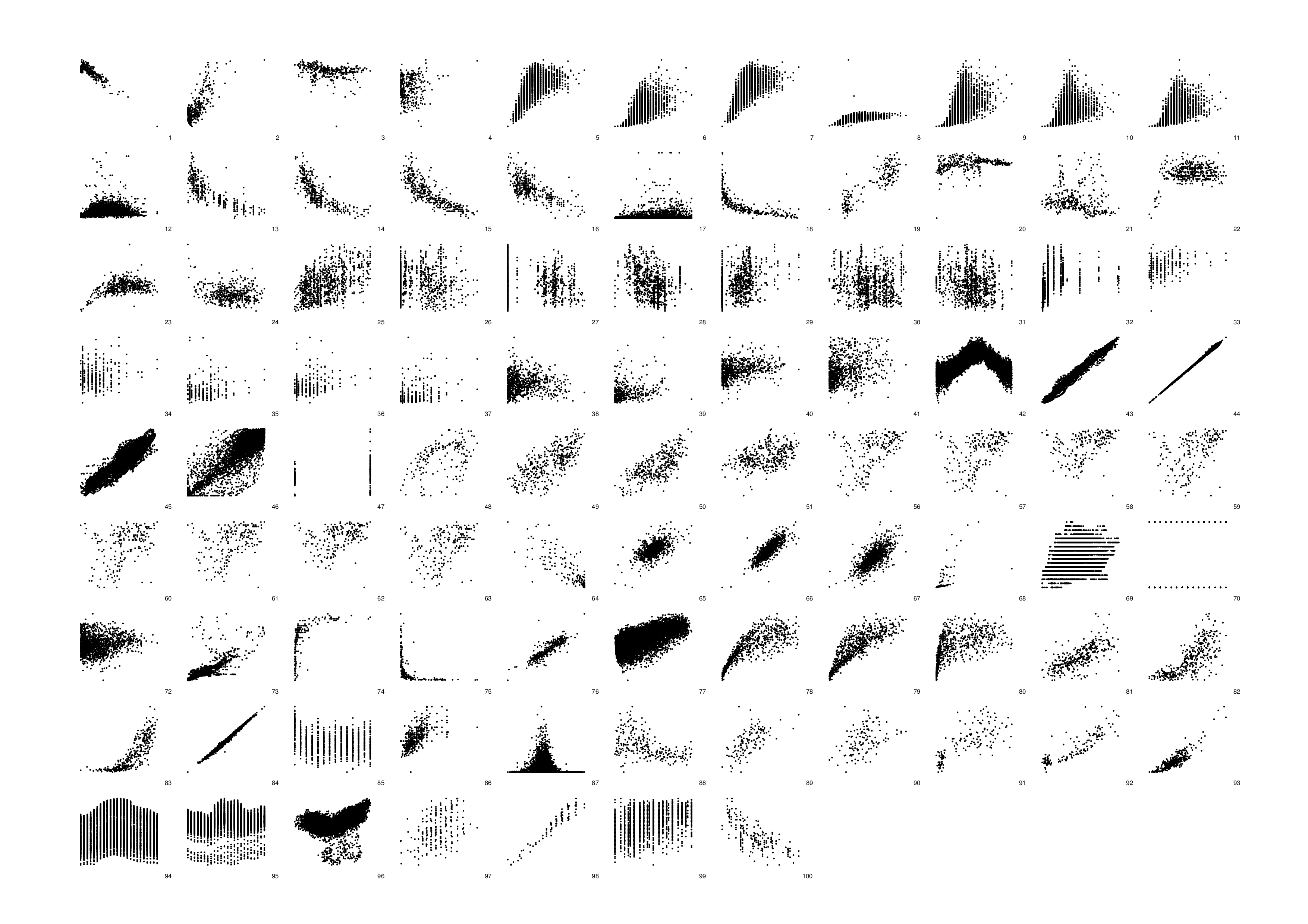
Figure 6: Scatter plots of the cause-effect pairs in the CauseEffectPairs benchmark data. We only show the pairs for which both variables are one-dimensional.

4.2.2 Simulated data

As collecting real-world benchmark data is a tedious process (mostly because the ground truths are unknown, and acquiring the necessary understanding of the data-generating process in order to decide about the ground truth is not straightforward), we also studied the performance of methods on simulated data where we can control the data-generating process, and therefore can be certain about the ground truth.

Simulating data can be done in many ways. It is not straightforward to simulate data in a “realistic” way, e.g., in such a way that scatter plots of simulated data look similar to those of the real-world data (see Figure 6). For reproducibility, we describe in Appendix C in detail how the simulations were done. Here, we will just sketch the main ideas.

We sample data from the following structural equation models. If we do not want to model a confounder, we use:

$$E_{X}\sim p_{E_{X}},\,E_{Y}\sim p_{E_{Y}}$$

$$X=f_{X}(E_{X})$$

$$Y=f_{Y}(X,E_{Y}),$$

and if we do want to include a confounder $Z$, we use:

$$E_{X}\sim p_{E_{X}},\,E_{Y}\sim p_{E_{Y}},\,E_{Z}\sim p_{E_{Z}}$$

$$Z=f_{Z}(E_{Z})$$

$$X=f_{X}(E_{X},E_{Z})$$

$$Y=f_{Y}(X,E_{Y},E_{Z}).$$

Here, the noise distributions $p_{E_{X}},p_{E_{Y}},p_{E_{Z}}$ are randomly generated distributions, and the causal mechanisms $f_{Z},f_{X},f_{Y}$ are randomly generated functions. Sampling the random distributions for a noise variable $E_{X}$ (and similarly for $E_{Y}$ and $E_{Z}$) is done by mapping a standard-normal distribution through a random function, which we sample from a Gaussian Process. The causal mechanism $f_{X}$ (and similarly $f_{Y}$ and $f_{Z}$) is drawn from a Gaussian Process as well. After sampling the noise distributions and the functional relations, we generate data for $X,Y,Z$. Finally, Gaussian measurement noise is added to both $X$ and $Y$.

By controlling various hyperparameters, we can control certain aspects of the data generation process. We considered four different scenarios. SIM is the default scenario without confounders. SIM-c includes a one-dimensional confounder, whose influences on $X$ and $Y$ are typically equally strong as the influence of $X$ on $Y$. The setting SIM-ln has low noise levels, and we would expect IGCI to work well in this scenario. Finally, SIM-G has approximate Gaussian distributions for the cause $X$ and approximately additive Gaussian noise (on top of a nonlinear relationship between cause and effect); we expect that methods which make these Gaussianity assumptions will work well in this scenario. Scatter plots of the simulated data are shown in Figures 7–10.

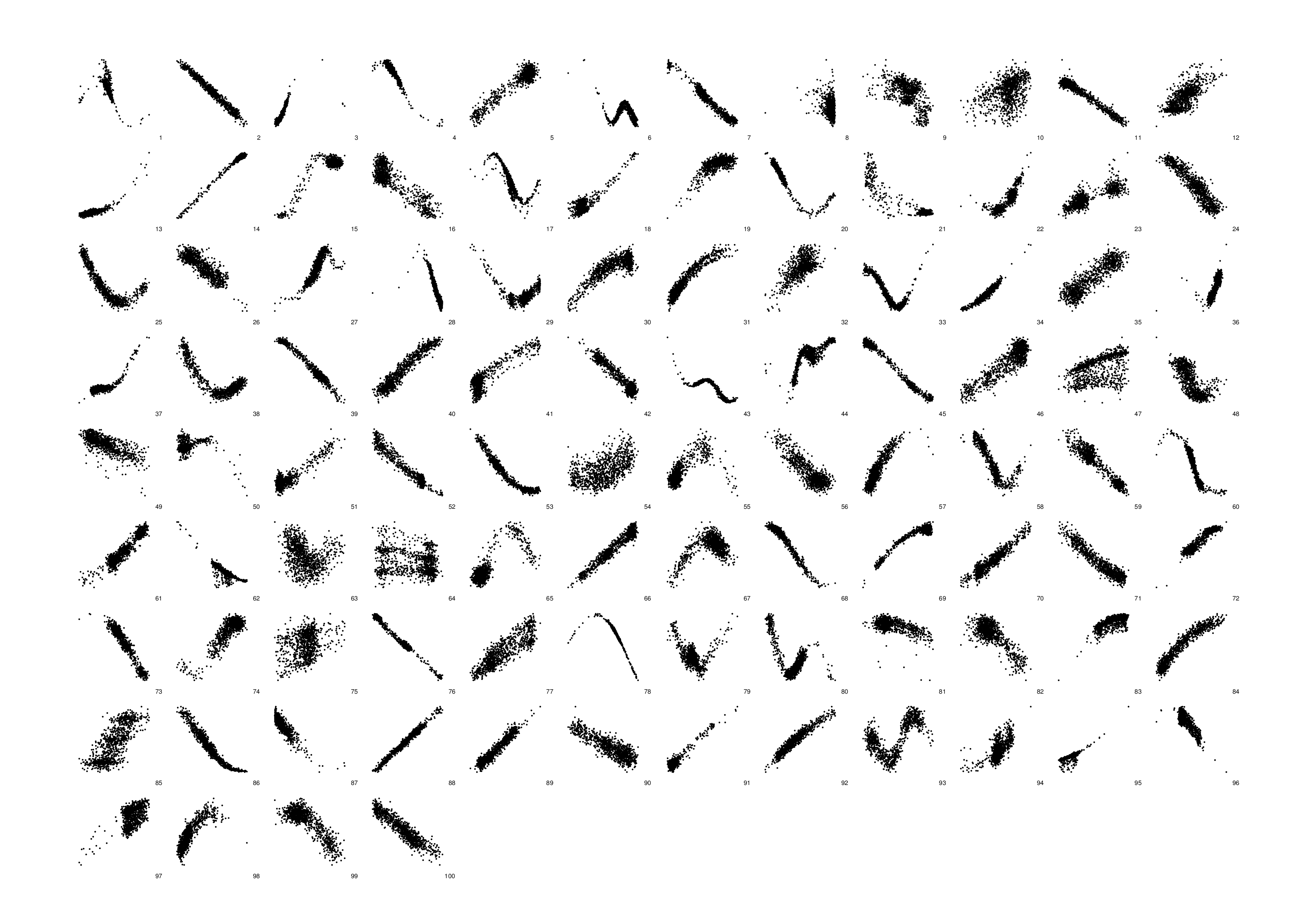
Figure 7: Scatter plots of the cause-effect pairs in simulation scenario SIM.

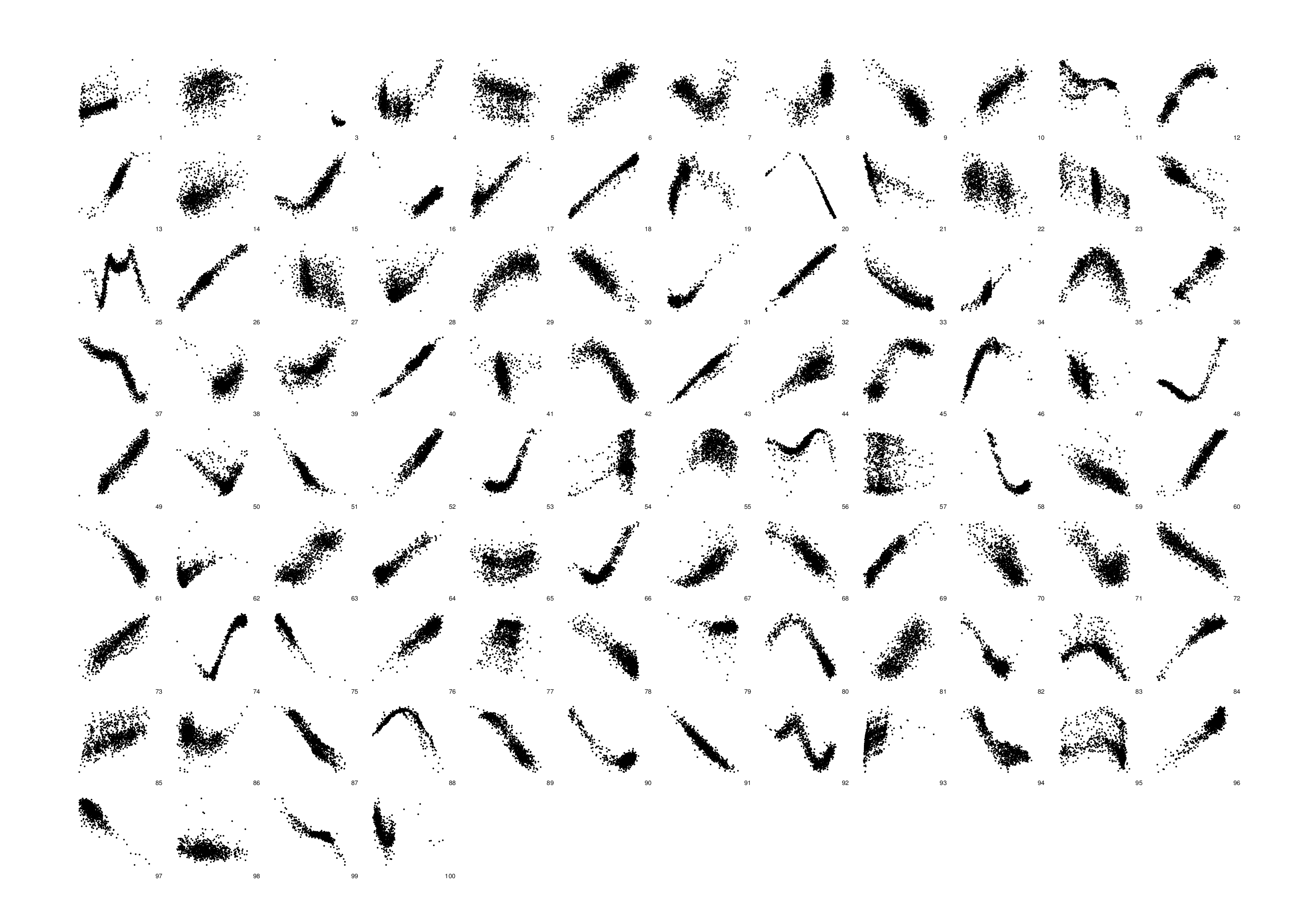
Figure 8: Scatter plots of the cause-effect pairs in simulation scenario SIM-c.

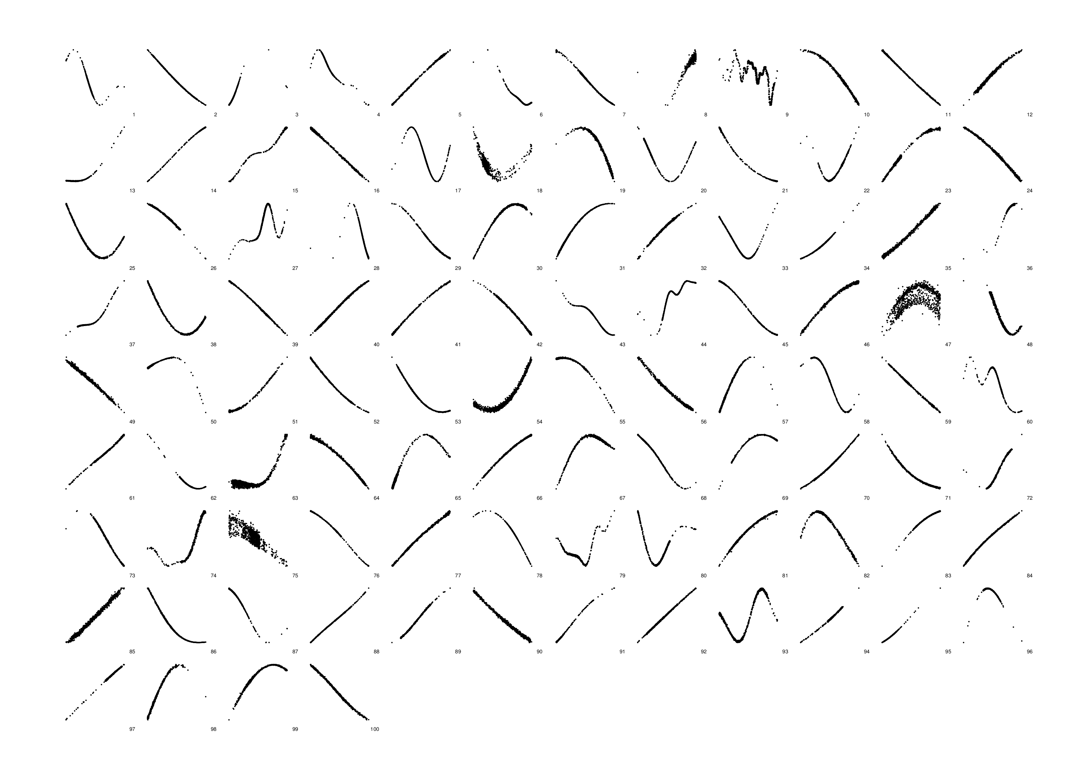
Figure 9: Scatter plots of the cause-effect pairs in simulation scenario SIM-ln.

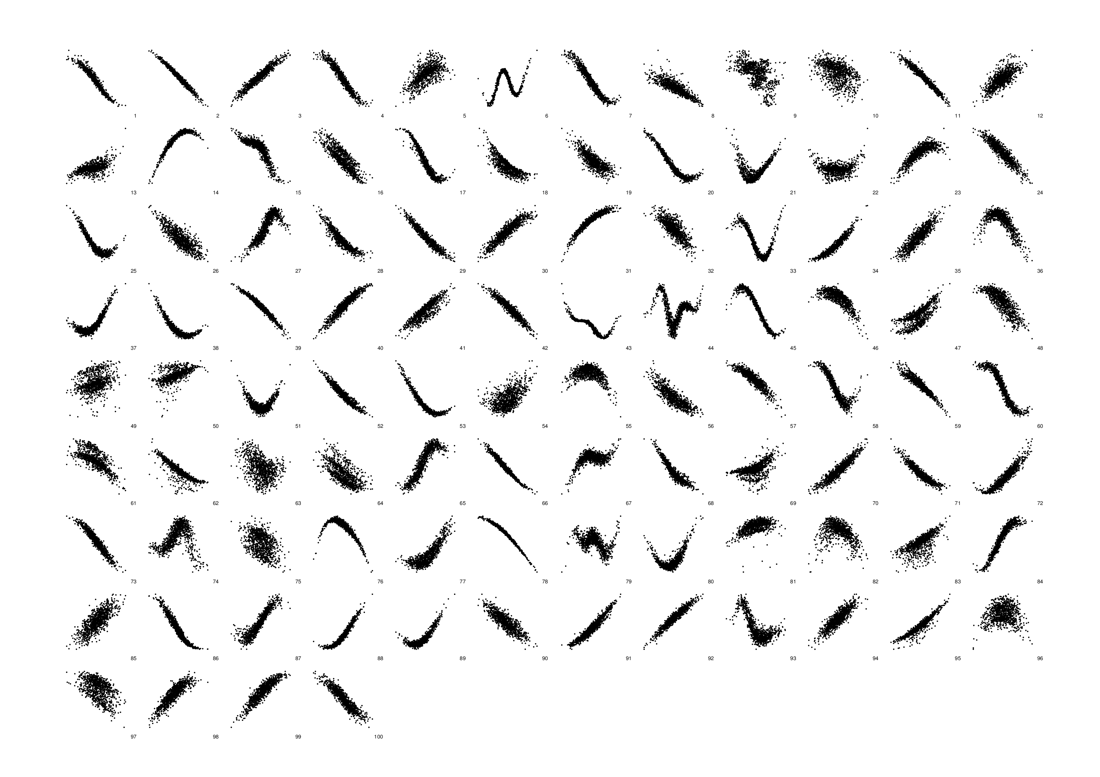
Figure 10: Scatter plots of the cause-effect pairs in simulation scenario SIM-G.

4.3 Preprocessing and Perturbations

The following preprocessing was applied to each pair $(X,Y)$. Both variables $X$ and $Y$ were standardized (i.e., an affine transformation is applied on both variables such that their empirical mean becomes 0, and their empirical standard deviation becomes 1). In order to study the effect of discretization and other small perturbations of the data, one of these four perturbations was applied:

unperturbed

: No perturbation is applied.

discretized

: Discretize the variable that has the most unique values such that after discretization, it has as many unique values as the other variable. The discretization procedure repeatedly merges those values for which the sum of the absolute error that would be caused by the merge is minimized.

undiscretized

: “Undiscretize” both variables $X$ and $Y$. The undiscretization procedure adds noise to each data point $z$, drawn uniformly from the interval $[0,z^{\prime}-z]$, where $z^{\prime}$ is the smallest value $z^{\prime}>z$ that occurs in the data.

small noise

: Add tiny independent Gaussian noise to both $X$ and $Y$ (with mean 0 and standard deviation $10^{-9}$).

Ideally, a causal discovery method should be robust against these and other small perturbations of the data.

4.4 Evaluation Measures

We evaluate the performance of the methods in two different ways:

forced-decision

: given a sample of a pair $(X,Y)$ the methods have to decide either $X\to Y$ or $Y\to X$; in this setting we evaluate the accuracy of these decisions;

ranked-decision

: we used the scores $\hat{C}_{X\to Y}$ and $\hat{C}_{Y\to X}$ to construct heuristic confidence estimates that are used to rank the decisions; we then produced receiver-operating characteristic (ROC) curves and used the area under the curve (AUC) as performance measure.

Some methods have an advantage in the second setting, as the scores on which their decisions are based yield a reasonably accurate ranking of the decisions. By only taking the most confident (highest ranked) decisions, the accuracy of these decisions increases, and this leads to a higher AUC than for random confidence estimates. Which of the two evaluation measures (accuracy or AUC) is the most relevant depends on the application.

4.4.1 Weights

For the CEP data, we cannot always consider pairs that come from the same data set as independent. For example, in the case of the Abalone data set (Bache and Lichman, 2013; Nash et al., 1994), the variables “whole weight”, “shucked weight”, “viscera weight”, “shell weight” are strongly correlated. Considering the four pairs (age, whole weight), (age, shucked weight), etc., as independent could introduce a bias. We (conservatively) correct for that bias by downweighting these pairs. In general, we chose the weights such that the weights of all pairs from the same data set are equal and sum to one. For the real-world cause-effect pairs, the weights are specified in Table LABEL:tab:CEP_pairs. For the simulated pairs, we do not use weighting.

4.4.2 Forced-decision: evaluation of accuracy

In the “forced-decision” setting, we calculate the weighted accuracy of a method in the following way:

$$\mathrm{accuracy}=\frac{\sum_{m=1}^{M}w_{m}\delta_{\hat{d}_{m},d_{m}}}{\sum_{m=1}^{M}w_{m}},$$ (26)

where $d_{m}$ is the true causal direction for the $m$’th pair (either “$\leftarrow$” or “$\rightarrow$”), $\hat{d}_{m}$ is the estimated direction (one of “$\leftarrow$”, “$\rightarrow$”, and “?”), and $w_{m}$ is the weight of the pair. Note that we are only awarding correct decisions, i.e., if no estimate is given ($d_{m}=\text{``?''}$), this will negatively affect the accuracy. We calculate confidence intervals assuming a binomial distribution using the method by Clopper and Pearson (1934).

4.4.3 Ranked-decision: evaluation of AUC

To construct an ROC curve, we need to rank the decisions based on some heuristic estimate of confidence. For most methods we simply use:

$$\hat{S}:=-\hat{C}_{X\to Y}+\hat{C}_{Y\to X}.$$ (27)

The interpretation is that the higher $\hat{S}$, the more likely $X\to Y$, and the lower $\hat{S}$, the more likely $Y\to X$. For ANM-pHSIC, we use a different heuristic:

$$\hat{S}:=\begin{cases}\frac{-1}{\min\{\hat{C}_{X\to Y},\hat{C}_{Y\to X}\}}&\text{ if }\hat{C}_{X\to Y}<\hat{C}_{Y\to X}\\ \frac{1}{\min\{\hat{C}_{X\to Y},\hat{C}_{Y\to X}\}}&\text{ if }\hat{C}_{X\to Y}>\hat{C}_{Y\to X},\\ \end{cases}$$ (28)

and for ANM-HSIC, we use:

$$\hat{S}:=\begin{cases}\frac{-1}{1-\min\{\hat{C}_{X\to Y},\hat{C}_{Y\to X}\}}&\text{ if }\hat{C}_{X\to Y}<\hat{C}_{Y\to X}\\ \frac{1}{1-\min\{\hat{C}_{X\to Y},\hat{C}_{Y\to X}\}}&\text{ if }\hat{C}_{X\to Y}>\hat{C}_{Y\to X}.\\ \end{cases}$$ (29)

In the “ranked-decision” setting, we also use weights to calculate weighted recall (depending on a threshold $\theta$)

$$\mathrm{recall}(\theta)=\frac{\sum_{m=1}^{M}w_{m}\mathbf{1}_{\hat{S}_{m}>\theta}\delta_{d_{m},\rightarrow}}{\sum_{m=1}^{M}w_{m}\delta_{d_{m},\rightarrow}},$$ (30)

where $\hat{S}_{m}$ is the heuristic score of the $m$’th pair (high values indicating high likelihood that $d_{m}={}\rightarrow$, low values indicating high likelihood that $d_{m}={}\leftarrow$), and the weighted precision (also depending on $\theta$)

$$\mathrm{precision}(\theta)=\frac{\sum_{m=1}^{M}w_{m}\mathbf{1}_{\hat{S}_{m}>\theta}\delta_{d_{m},\rightarrow}}{\sum_{m=1}^{M}w_{m}\mathbf{1}_{\hat{S}_{m}>\theta}}.$$ (31)

We use the MatLab routine perfcurve to produce (weighted) ROC curves and to estimate weighted AUC and confidence intervals for the weighted AUC by bootstrapping.

5 Results

In this section, we report the results of the experiments that we carried out in order to evaluate the performance of various methods. We plot the accuracies and AUCs as box plots, indicating the estimated (weighted) accuracy or AUC, the corresponding $68\%$ confidence interval, and the $95\%$ confidence interval. If there were pairs for which no decision was taken because of some failure, the number of nondecisions is indicated on the corresponding boxplot. The methods that we evaluated are listed in Table 2. Computation times are reported in Appendix E.

Table 2: The methods that are evaluated in this work.

Name	Algorithm	Score	Heuristic	Details
ANM-pHSIC	1	(5)	(28)	Data recycling, adaptive kernel bandwidth
ANM-HSIC	1	(6)	(29)	Data recycling, adaptive kernel bandwidth
ANM-HSIC-ds	1	(6)	(29)	Data splitting, adaptive kernel bandwidth
ANM-HSIC-fk	1	(6)	(29)	Data recycling, fixed kernel bandwidth (0.5)
ANM-HSIC-ds-fk	1	(6)	(29)	Data splitting, fixed kernel bandwidth (0.5)
ANM-ent-…	1	(9)	(27)	Data recycling, entropy estimators from Table 1
ANM-Gauss	1	(11)	(27)	Data recycling
ANM-FN	2	(12)	(27)
ANM-MML	2	(13)	(27)
IGCI-slope	3	(21)	(27)
IGCI-slope++	3	(23)	(27)
IGCI-ent-…	3	(22)	(27)	Entropy estimators from Table 1

5.1 Additive Noise Models

We start by reporting the results for methods that exploit additivity of the noise. Figure 11 shows the performance of all ANM methods on different unperturbed data sets, i.e., the CEP benchmark and various simulated data sets. Figure 12 shows the performance of the same methods on different perturbations of the CEP benchmark data. The six variants sp1,…,sp6 of the spacing estimators perform very similarly, so we show only the results for ANM-ent-sp1. For the “undiscretized” perturbed version of the CEP benchmark data, GP regression failed in one case because of a numerical problem, which explains the failures across all methods in Figure 12 for that case.

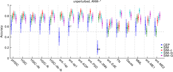
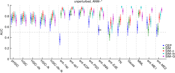
Figure 11: Accuracies (top) and AUCs (bottom) of various ANM methods on different (unperturbed) data sets. For the variants of the spacing estimator, only the results for sp1 are shown, as results for sp2,…,sp6 were similar.

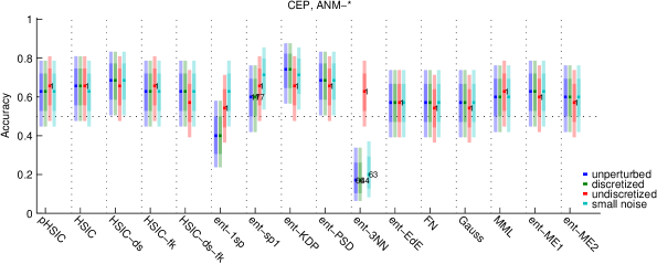
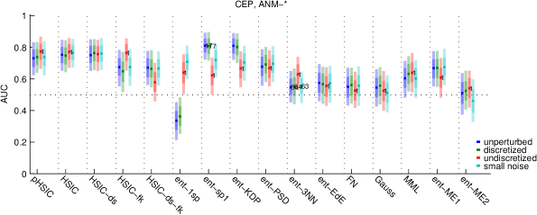
Figure 12: Accuracies (top) and AUCs (bottom) of various ANM methods on different perturbations of the CEP benchmark data. For the variants of the spacing estimator, only the results for sp1 are shown, as results for sp2,…,sp6 were similar.

5.1.1 HSIC-based scores

As we see in Figure 11 and Figure 12, the ANM methods that use HSIC perform reasonably well on all data sets, obtaining accuracies between 63% and 85%. Note that the simulated data (and also the real-world data) deviate in at least three ways from the assumptions made by the additive noise method: (i) the noise is not additive, (ii) a confounder can be present, and (iii) additional measurement noise was added to both cause and effect. Moreover, the results turn out to be robust against small perturbations of the data. This shows that the additive noise method can perform reasonably well, even in case of model misspecification.

The results of ANM-pHSIC and ANM-HSIC are very similar. The influence of various implementation details on performance is small. On the CEP benchmark, data-splitting (ANM-HSIC-ds) slightly increases accuracy, whereas using a fixed kernel (ANM-HSIC-fk, ANM-HSIC-ds-fk) slightly lowers AUC. Generally, the differences in performance are small and not statistically significant. The variant ANM-HSIC-ds-fk is proved to be consistent in Appendix A. If standard GP regression satisfies the property in (38), then ANM-HSIC-fk is also consistent.

5.1.2 Entropy-based scores

For the entropy-based score (9), we see in Figure 11 and Figure 12 that the results depend strongly on which entropy estimator is used.

All (nonparametric) entropy estimators (1sp, 3NN, spi, KDP, PSD) perform well on simulated data, with the exception of EdE. On the CEP benchmark on the other hand, the performance varies greatly over estimators. One of the reasons for this are discretization effects. Indeed, the differential entropy of a variable that can take only a finite number of values is $-\infty$. The way in which differential entropy estimators treat values that occur multiple times differs, and this can have a large influence on the estimated entropy. For example, 1sp simply ignores values that occur more than once, which leads to a performance that is below chance level on the CEP data. 3NN returns $-\infty$ (for both $\hat{C}_{X\to Y}$ and $\hat{C}_{Y\to X}$) in the majority of the pairs in the CEP benchmark and therefore often cannot decide. The spacing estimators spi also return $-\infty$ in quite a few cases. The only (nonparametric) entropy-based ANM methods that perform well on both the CEP benchmark data and the simulated data are ANM-ent-KDP and ANM-ent-PSD. Of these two methods, ANM-ent-PSD seems more robust under perturbations than ANM-ent-KDP, and can compete with the HSIC-based methods.

5.1.3 Other scores

Consider now the results for the “parametric” entropy estimators (ANM-Gauss, ANM-ent-ME1, ANM-ent-ME2), the empirical-Bayes method ANM-FN, and the MML method ANM-MML.

First, note that ANM-Gauss and ANM-FN perform very similarly. This means that the difference between these two scores (i.e., the complexity measure of the regression function, see also Appendix B) does not outweigh the common part (the likelihood) of these two scores. Both these scores do not perform much better than chance on the CEP data, probably because the Gaussianity assumption is typically violated in real data. They do obtain high accuracies and AUCs for the SIM-ln and SIM-G scenarios. For SIM-G this is to be expected, as the assumption that the cause has a Gaussian distribution is satisfied in that scenario. For SIM-ln it is not evident why these scores perform so well—it could be that the noise is close to additive and Gaussian in that scenario.

The related score ANM-MML, which employs a more sophisticated complexity measure for the distribution of the cause, performs better on the two simulation settings SIM and SIM-c. However, ANM-MML performs worse in the SIM-G scenario, which is probably due to a higher variance of the MML complexity measure compared with the simple Gaussian entropy measure. This is in line with expectations. However, performance of ANM-MML is hardly better than chance on the CEP data. In particular, the AUC of ANM-MML is worse than that of ANM-pHSIC.

The parametric entropy estimators ME1 and ME2 do not perform very well on the SIM data, although their performance on the other simulated data sets (in particular SIM-G) is good. The reasons for this behaviour are not understood; we speculate that the parametric assumptions made by these estimators match the actual distribution of the data in these particular simulation settings quite well. The accuracy and AUC of ANM-ent-ME1 and ANM-ent-ME2 on the CEP data are lower than those of ANM-pHSIC.

5.2 Information Geometric Causal Inference

Here we report the results of the evaluation of different IGCI variants. Figure 13 shows the performance of all the IGCI variants on different (unperturbed) data sets, the CEP benchmark and four different simulation settings, using the uniform base measure. Figure 14 shows the same for the Gaussian base measure. Figure 15 shows the performance of the IGCI methods on different perturbations of the CEP benchmark, using the uniform base measure, and Figure 16 for the Gaussian base measure. Again, the six variants sp1,…,sp6 of the spacing estimators perform very similarly, so we show only the results for IGCI-ent-sp1.

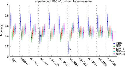
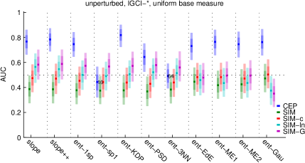
Figure 13: Accuracies (top) and AUCs (bottom) for various IGCI methods using the uniform base measure on different (unperturbed) data sets.

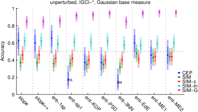
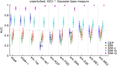
Figure 14: Accuracies (top) and AUCs (bottom) for various IGCI methods using the Gaussian base measure on different (unperturbed) data sets.

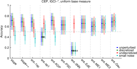
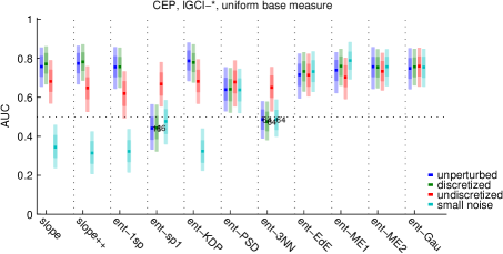
Figure 15: Accuracies (top) and AUCs (bottom) for various IGCI methods using the uniform base measure on different perturbations of the CEP benchmark data.

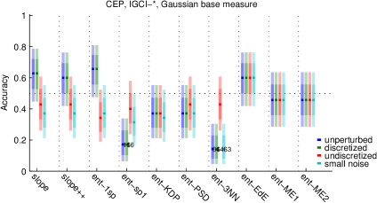
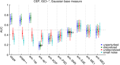
Figure 16: Accuracies (top) and AUCs (bottom) for various IGCI methods using the Gaussian base measure on different perturbations of the CEP benchmark data.

Let us first look at the performance on simulated data. Note that none of the IGCI methods performs well on the simulated data when using the uniform base measure. A very different picture emerges when using the Gaussian base measure: here the performance covers a wide spectrum, from lower than chance level on the SIM data to accuracies higher than 90% on SIM-G. The choice of the base measure clearly has a larger influence on the performance than the choice of the estimation method.

As IGCI was designed for the bijective deterministic case, one would expect that IGCI would work best on SIM-ln (without depending too strongly on the reference measure), because in that scenario the noise is relatively small. Surprisingly, this does not turn out to be the case. To understand this unexpected behavior, we inspect the scatter plots in Figure 9 and observe that the functions in SIM-ln are either non-injective or relatively close to linear. Both can spoil the performance despite having low noise (see also the remarks at the end of Subsection 3.2 on finite sample effects).

For the more noisy settings, earlier experiments showed that IGCI-slope and IGCI-1sp can perform surprisingly well on simulated data (Janzing et al., 2012). Here, however, we see that the performance of all IGCI variants on noisy data depends strongly on characteristics of the data generation process and on the chosen base measure. IGCI seems to pick up certain features in the data that turn out to be correlated with the causal direction in some settings, but can be anticorrelated with the causal direction in other settings. In addition, our results suggest that if the distribution of the cause is close to the base measure used in IGCI, then also for noisy data the method may work well (as in the SIM-G setting). However, for causal relations that are not sufficiently non-linear, performance can drop significantly (even below chance level) in case of a discrepancy between the actual distribution of the cause and the base measure assumed by IGCI.

Even though the performance of all IGCI variants with uniform base measure is close to chance level on the simulated data, most methods perform better than chance on the CEP data (with the exception of IGCI-ent-sp1 and IGCI-ent-3NN). When using the Gaussian base measure, performance of IGCI methods on CEP data varies considerably depending on implementation details. For some IGCI variants the performance on CEP data is robust to small perturbations (most notably the parametric entropy estimators), but for most non-parametric entropy estimators and for IGCI-slope, there is a strong dependence and sometimes even an inversion of the accuracy when perturbing the data slightly. We do not have a good explanation for these observations.

5.2.1 Original implementations

Let us now take a closer look at the accuracies of the original methods IGCI-slope and IGCI-ent-1sp that were proposed in (Daniušis et al., 2010; Janzing et al., 2012), and at the newly introduced IGCI-slope++ that is closely related to IGCI-slope. The IGCI variants slope, slope++ and ent-1sp perform very similar on all data sets. For both uniform and Gaussian base measures, the performance is better than chance level on the CEP benchmark, but not as much as in previous evaluations on earlier versions of the benchmark. The discrepancy with the accuracies of around 80% reported by Janzing et al. (2012) could be explained by the fact that here we evaluate on a larger set of cause-effect pairs, and we chose the weights more conservatively.

It is also interesting to look at the behavior under perturbations of the CEP data. When using the uniform base measure, the accuracy of both IGCI-slope and IGCI-ent-1sp drops back to chance level if small noise is added, whereas AUC even becomes worse than chance level. For the Gaussian base measure, both accuracy and AUC become worse than random guessing on certain perturbations of the CEP data, although discretization does not affect performance. This observation motivated the introduction of the slope-based estimator IGCI-slope++ that uses (23) instead of (21) in order to deal better with repetitions of values. However, as we can see, this estimator does not perform better in practice than the original estimator IGCI-slope.

5.2.2 Nonparametric entropy estimators

It is clear that discretization effects play an important role in the performance of the nonparametric entropy estimators. For example, the closely related estimators 1sp and spi perform comparably on simulated data, but on the CEP data, the spi estimators perform worse because of nondecisions due to repeated values. Similarly, the bad performance of IGCI-ent-3NN on the CEP data is related to discretization effects. This is in line with our observations on the behavior of these entropy estimators when using them for entropy-based ANM methods.

Further, note that the performance of IGCI-ent-KDP is qualitatively similar to that of IGCI-ent-PSD, but in contrast with the PSD estimator, the results of the KDP estimator are not robust under perturbations when using the uniform base measure. The only nonparametric entropy estimators that give results that are robust to small perturbations of the data (for both base measures) are PSD and EdE. The performance of IGCI-ent-PSD on the CEP benchmark depends on the chosen base measure: for the uniform base it is better than chance level, for the Gaussian base measure it is worse than chance level. Interestingly, the EdE estimator that performed poorly for ANM gives consistently good results on the CEP benchmark when used for IGCI: it is the only nonparametric entropy estimator that yields results that are better than chance for both base measures and irrespectively of whether the data were perturbed or not.

Apparently, implementation details of entropy estimators can result in huge differences in performance, often in ways that we do not understand well.

5.2.3 Parametric entropy estimators

Let us finally consider the performance of entropy-based IGCI methods that use parametric entropy estimators, which make additional assumptions on the distribution. As expected, these estimators are robust to small perturbations of the data.

Interestingly, IGCI-ent-Gau with uniform base measure turns out to be one of the best IGCI methods on the CEP benchmark, in the sense that it obtains good accuracy and AUC and in addition is robust to perturbations. Note that the performance of IGCI-ent-Gau on the CEP benchmark is comparable with that of the original implementation IGCI-slope and the newer version IGCI-slope++, but that only IGCI-ent-Gau is robust to small perturbations of the data. This estimator simply estimates entropy by assuming a Gaussian distribution. In other words, it uses:

$$\hat{C}_{X\to Y}:=\frac{1}{2}\log\widehat{\mathbb{V}\mathrm{ar}}(\tilde{\bm{y}})-\frac{1}{2}\log\widehat{\mathbb{V}\mathrm{ar}}(\tilde{\bm{x}})=\log\left(\frac{\sqrt{\widehat{\mathbb{V}\mathrm{ar}(\bm{y})}}}{\max(\bm{y})-\min(\bm{y})}\Bigg{/}\frac{\sqrt{\widehat{\mathbb{V}\mathrm{ar}(\bm{x})}}}{\max(\bm{x})-\min(\bm{x})}\right).$$

Apparently, the ratio of the size of the support of the distribution and its standard deviation is already quite informative on the causal direction for the CEP data. This might also explain the relatively good performance on this benchmark of IGCI-ent-ME1 and IGCI-ent-ME2 when using the uniform base measure, as these estimate entropy by fitting a parametric distribution to the data (which includes Gaussian distributions as a special case). On the other hand, these methods do not work better than chance on the simulated data.

Now let us look at the results when using the Gaussian base measure. IGCI-ent-Gau makes no sense in combination with the Gaussian base measure. IGCI-ent-ME1 and IGCI-ent-ME2 on the CEP data do not perform better than chance. On simulated data, they only do (extremely) well for the SIM-G scenario which uses a Gaussian distribution of the cause measure, i.e., for which the chosen base measure exactly corresponds with the distribution of the cause.

6 Discussion and Conclusion

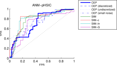
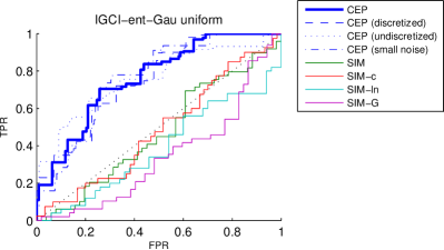
Figure 17: ROC curves for two of the best-performing methods (ANM-pHSIC and IGCI-ent-Gau). Both methods work well on the CEP benchmark and keep performing well under small perturbations of the data, but only ANM-pHSIC also performs well on the simulated data.

In this work, we considered a challenging bivariate causal discovery problem, where the task is to decide whether $X$ causes $Y$ or vice versa, using only a sample of purely observational data. We reviewed two families of methods that can be applied to this task: Additive Noise Methods (ANM) and Information Geometric Causal Inference (IGCI) methods. We discussed various possible implementations of these methods and how they are related.

In addition, we have proposed the CauseEffectPairs benchmark data set consisting of 100 real-world cause-effect pairs and we provided our justifications for the ground truths. We have used this benchmark data in combination with several simulated data sets in order to evaluate various bivariate causal discovery methods. Our main conclusions (illustrated in Figure 17) are twofold:

1. The ANM methods that use HSIC perform reasonably well on all data sets (including the perturbed versions of the CEP benchmark and all simulation settings), obtaining accuracies between 63% and 85% (see Figures 11 and 12). In particular, the original ANM-pHSIC method obtains an accuracy of 63 $\pm$ 10 % and an AUC of 0.74 $\pm$ 0.05 on the CEP benchmark. The only other ANM method that performs well on all data sets is ANM-ent-PSD. It obtains a higher accuracy (69 $\pm$ 10%) than ANM-pHSIC on the CEP benchmark, but a lower AUC (0.68 $\pm$ 0.06), but these differences are not statistically significant.

2. The performance of IGCI-based methods varies greatly depending on implementation details, perturbations of the data and certain characteristics of the data, in ways that we do not fully understand (see Figures 13, 14, 15, 16). In many cases, causal relations seem to be too linear for IGCI to work well. None of the IGCI implementations performed well on all data sets that we considered, and the apparent better-than-chance performance of some of these methods on the CEP benchmark remains somewhat of a mystery.

The former conclusion about the performance of ANM-pHSIC is in line with earlier reports, but the latter conclusion is surprising, considering that good performance of IGCI-slope and IGCI-ent-1sp has been reported on several occassions in earlier work (Daniušis et al., 2010; Mooij et al., 2010; Janzing et al., 2012; Statnikov et al., 2012; Sgouritsa et al., 2015). One possible explanation that the performance of IGCI on simulated data here differs from earlier reports is that earlier simulations used considerably smoother distributions of the cause variable.

Ironically, the original ANM method ANM-pHSIC proposed by Hoyer et al. (2009) turned out to be one of the best methods overall, despite the recent research efforts aimed at developing better methods. This observation motivated the consistency proof of HSIC-based ANM methods, the major theoretical contribution of this work. We expect that extending this consistency result to the multivariate case (see also Peters et al., 2014) should be straightforward.

One reason for the disappointing performance of several methods (in particular, the slope-based IGCI estimators and methods that make use of certain nonparametric differential entropy estimators) is discretization. When dealing with real-world data on a computer, variables of a continuous nature are usually discretized because they have to be represented as floating point numbers. Often, additional rounding is applied, for example because only the most significant digits are recorded. We found that for many methods, especially for those that use differential entropy estimators, (coarse) discretization of the data causes problems. This suggests that performance of several methods can still be improved, e.g., by using entropy estimators that are more robust to such discretization effects. The HSIC independence measure (and its $p$-value) and the PSD entropy estimator were found to be robust against small perturbations of the data, including discretization.

Since we compared many different implementations (which turned out to have quite different performance characteristics), we need to use a strong correction for multiple testing if we would like to conclude that one of these methods performs significantly better than chance. Although it seems unlikely that the good performance of ANM-pHSIC on both CEP data and all simulated data is due to chance alone, eventually we are most interested in the performance on real-world data alone. Unfortunately, the CEP benchmark turned out to be too small to warrant significant conclusions for any of the tested methods.

A rough estimate how large the CauseEffectPairs benchmark should have been in order to obtain significant results can easily be made. Using a standard (conservative) Bonferroni correction, taking into account that we compared 37 methods, we would need about 120 (weighted) pairs for an accuracy of 65% to be considered significant (with two-sided testing and 5% significance threshold). This is about four times as much as the current number of 37 (weighted) pairs in the CauseEffectPairs benchmark. Therefore, we suggest that at this point, the highest priority regarding future work should be to obtain more validation data, rather than developing additional methods or optimizing computation time of existing methods. We hope that our publication of the CauseEffectPairs benchmark data inspires researchers to collaborate on this important task and we invite everybody to contribute pairs to the CauseEffectPairs benchmark data.

Concluding, our results provide some evidence that distinguishing cause from effect is indeed possible from purely observational real-world data by exploiting certain statistical patterns in the data. However, the performance of current state-of-the-art bivariate causal discovery methods still has to be improved further in order to enable practical applications, and more validation data are needed in order to obtain statistically significant conclusions. Furthermore, it is not clear at this stage under what assumptions current methods could be extended to deal with possible confounding variables, an important issue in practice.

A Consistency Proof of ANM-HSIC

In this Appendix, we prove the consistency of Algorithm 1 with score (7), which is closely related to the algorithm originally proposed by Hoyer et al. (2009) that uses score (5). The main difference is that the original implementation uses the HSIC $p$-value, whereas here, we use the HSIC value itself as a score. Also, we consider the option of splitting the dataset into one part for regression and another part for independence testing. Finally, we fix the HSIC kernel instead of letting its bandwidth be chosen by a heuristic that depends on the data. The reason that we make these small modifications is that they lead to an easier proof of consistency of the method.

We start with recapitulating the definition and basic properties of the Hilbert Schmidt Independence Criterion (HSIC) in Section A.1. Then, we discuss asymptotic properties of non-parametric regression methods in Section A.2. Finally, we combine these ingredients in Section A.3.

A.1 Consistency of HSIC

We recapitulate the definitions and some asymptotic properties of the Hilbert Schmidt Independence Criterion (HSIC), following mostly the notations and terminology in (Gretton et al., 2005). The HSIC estimator that we use here is the original biased estimator proposed by Gretton et al. (2005).

Definition 11

Given two random variables $X\in\mathcal{X}$ and $Y\in\mathcal{Y}$ with joint distribution $\mathbb{P}_{X,Y}$, and bounded kernels $k:\mathcal{X}^{2}\to\mathbb{R}$ and $l:\mathcal{Y}^{2}\to\mathbb{R}$, we define the population HSIC of $X$ and $Y$ as:

$$\begin{split}\mathrm{HSIC}_{k,l}(X,Y):=&\mathbb{E}\big{(}k(X,X^{\prime})l(Y,Y^{\prime})\big{)}+\mathbb{E}\big{(}k(X,X^{\prime})\big{)}\mathbb{E}\big{(}l(Y,Y^{\prime})\big{)}\\ &-2\mathbb{E}\Big{(}\mathbb{E}\big{(}k(X,X^{\prime})\,|\,X\big{)}\mathbb{E}\big{(}l(Y,Y^{\prime})\,|\,Y\big{)}\Big{)}\end{split}$$

Here, $(X,Y)$ and $(X^{\prime},Y^{\prime})$ are two independent random variables distributed according to $\mathbb{P}_{X,Y}$.

When $k$ and $l$ are clear from the context, we will typically suppress the dependence of the population HSIC on the choice of the kernels $k$ and $l$, simply writing $\mathrm{HSIC}(X,Y)$ instead. The justification for the name “independence criterion” stems from the following important result (Fukumizu et al., 2008, Theorem 3):

Lemma 12

Whenever the product kernel $k\cdot l$ is characteristic (in the sense of (Fukumizu et al., 2008; Sriperumbudur et al., 2010)): $\mathrm{HSIC}_{k,l}(X,Y)=0$ if and only if $X\mbox{${}\perp\mkern-11.0mu\perp{}$}Y$ (i.e., $X$ and $Y$ are independent).  

A special case of this lemma, assuming that $X$ and $Y$ have compact domain, was proven originally in (Gretton et al., 2005). Recently, Gretton (2015) showed that a similar result also holds if both kernels $k$ and $l$ are characteristic and satisfy some other conditions as well. Intuitively, a characteristic kernel leads to an injective embedding of probability measures into the corresponding Reproducible Kernel Hilbert Space (RKHS). The HSIC is the squared RKHS distance between the embedded joint distribution and the embedded product of the marginals. Given that the embedding is injective, this distance is zero if and only if the variables are independent. Examples of characteristic kernels are Gaussian RBF kernels and Laplace kernels. For more details on the notion of characteristic kernel, see (Sriperumbudur et al., 2010). We will use the following (biased) estimator of the population HSIC (Gretton et al., 2005):

Definition 13

Given two $N$-tuples (with $N\geq 2$) $\bm{x}=(x_{1},\dots,x_{N})\in\mathcal{X}^{N}$ and $\bm{y}=(y_{1},\dots,y_{N})\in\mathcal{Y}^{N}$, and bounded kernels $k:\mathcal{X}^{2}\to\mathbb{R}$ and $l:\mathcal{Y}^{2}\to\mathbb{R}$, we define

$$\widehat{\mathrm{HSIC}}_{k,l}(\bm{x},\bm{y}):=(N-1)^{-2}\mathrm{tr}(KHLH)=(N-1)^{-2}\sum_{i,j=1}^{N}\bar{K}_{ij}L_{ij},$$ (32)

where $K_{ij}=k(x_{i},x_{j})$, $L_{ij}=l(y_{i},y_{j})$ are Gram matrices and $H_{ij}=\delta_{ij}-N^{-1}$ is a centering matrix, and we write $\bar{K}:=HKH$ for the centered Gram matrix $K$. Given an i.i.d. sample $\mathcal{D}_{N}=\{(x_{n},y_{n})\}_{n=1}^{N}$ from $\mathbb{P}_{X,Y}$, we define the empirical HSIC of $X$ and $Y$ estimated from $\mathcal{D}_{N}$ as:

$$\widehat{\mathrm{HSIC}}_{k,l}(X,Y;\mathcal{D}_{N}):=\widehat{\mathrm{HSIC}}_{k,l}(\bm{x},\bm{y}).$$

Again, when $k$ and $l$ are clear from the context, we will typically suppress the dependence of the empirical HSIC on the choice of the kernels $k$ and $l$. Unbiased estimators of the population HSIC were proposed in later work (Song et al., 2012), but we will not consider those here. A large deviation result for this empirical HSIC estimator is given by (Gretton et al., 2005, Theorem 3):

Lemma 14

Assume that kernels $k$ and $l$ are bounded almost everywhere by 1, and are non-negative. Suppose that the data set $\mathcal{D}_{N}$ consists of $N$ i.i.d. samples from some joint probability distribution $\mathbb{P}_{X,Y}$. Then, for $N\geq 2$ and all $\delta>0$, with probability at least $1-\delta$:

$$\left|\mathrm{HSIC}_{k,l}(X,Y)-\widehat{\mathrm{HSIC}}_{k,l}(X,Y;\mathcal{D}_{N})\right|\leq\sqrt{\frac{\log(6/\delta)}{\alpha^{2}N}}+\frac{c}{N},$$

where $\alpha^{2}>0.24$ and $c$ are constants.  

This directly implies the consistency of the empirical HSIC estimator:

Corollary 15

Let $(X_{1},Y_{1}),(X_{2},Y_{2}),\dots$ be i.i.d. according to $\mathbb{P}_{X,Y}$. Defining the sequence of data sets $\mathcal{D}_{N}=\{(X_{n},Y_{n})\}_{n=1}^{N}$ for $N=2,3,\dots$, we have for non-negative bounded kernels $k,l$ that, as $N\to\infty$:

$$\widehat{\mathrm{HSIC}}_{k,l}(X,Y;\mathcal{D}_{N})\stackrel{{\scriptstyle P}}{{\to}}\mathrm{HSIC}_{k,l}(X,Y).$$

 

We do not know of any results for consistency of HSIC when using adaptive kernel parameters (i.e., when estimating the kernel from the data). This is why we only present a consistency result for fixed kernels here.

For the special case that $\mathcal{Y}=\mathbb{R}$, we will use the following continuity property of the empirical HSIC estimator. It shows that for a Lipschitz-continuous kernel $l$, the empirical HSIC is also Lipschitz-continuous in the corresponding argument, but with a Lipschitz constant that scales at least as $N^{-1/2}$ for $N\to\infty$. This novel technical result will be the key to our consistency proof of Algorithm 1 with score (7).

Lemma 16

For all $N\geq 2$, for all $\bm{x}\in\mathcal{X}^{N}$, for all $\bm{y},\bm{y}^{\prime}\in\mathbb{R}^{N}$, for all bounded kernels $k:\mathcal{X}^{2}\to\mathbb{R}$, and for all bounded and Lipschitz-continuous kernels $l:\mathbb{R}^{2}\to\mathbb{R}$:

$$\left|\widehat{\mathrm{HSIC}}(\bm{x},\bm{y})-\widehat{\mathrm{HSIC}}(\bm{x},\bm{y}^{\prime})\right|\leq\frac{32\lambda C}{\sqrt{N}}\left\|{\bm{y}-\bm{y}^{\prime}}\right\|,$$

where $\left|k(\xi,\xi^{\prime})\right|\leq C$ for all $\xi,\xi^{\prime}\in\mathcal{X}$ and $\lambda$ is the Lipschitz constant of $l$.

Proof  From its definition, (32):

$$\left|\widehat{\mathrm{HSIC}}(\bm{x},\bm{y})-\widehat{\mathrm{HSIC}}(\bm{x},\bm{y}^{\prime})\right|=(N-1)^{-2}\left|\sum_{i,j=1}^{N}\bar{K}_{ij}(L_{ij}-L_{ij}^{\prime})\right|,$$

where $K_{ij}=k(x_{i},x_{j})$, $L_{ij}=l(y_{i},y_{j})$, $L_{ij}^{\prime}=l(y_{i}^{\prime},y_{j}^{\prime})$ and $\bar{K}:=HKH$ with $H_{ij}=\delta_{ij}-N^{-1}$. First, note that $\left|K_{ij}\right|\leq C$ implies that $\left|\bar{K}_{ij}\right|\leq 4C$:

$$\begin{split}\left|\bar{K}_{ij}\right|&=\left|K_{ij}-\frac{1}{N}\sum_{i^{\prime}=1}^{N}K_{i^{\prime}j}-\frac{1}{N}\sum_{j^{\prime}=1}^{N}K_{ij^{\prime}}+\frac{1}{N^{2}}\sum_{i^{\prime},j^{\prime}=1}^{N}K_{i^{\prime}j^{\prime}}\right|\\ &\leq\left|K_{ij}\right|+\frac{1}{N}\sum_{i^{\prime}=1}^{N}\left|K_{i^{\prime}j}\right|+\frac{1}{N}\sum_{j^{\prime}=1}^{N}\left|K_{ij^{\prime}}\right|+\frac{1}{N^{2}}\sum_{i^{\prime},j^{\prime}=1}^{N}\left|K_{i^{\prime}j^{\prime}}\right|\leq 4C.\end{split}$$

Now starting from the definition and using the triangle inequality:

$$\begin{split}\left|\sum_{i,j=1}^{N}\bar{K}_{ij}(L_{ij}-L_{ij}^{\prime})\right|\leq&\left|\sum_{i,j=1}^{N}\bar{K}_{ij}\big{(}l(y_{i}^{\prime},y_{j}^{\prime})-l(y_{i}^{\prime},y_{j})\big{)}\right|+\left|\sum_{i,j=1}^{N}\bar{K}_{ij}\big{(}l(y_{i}^{\prime},y_{j})-l(y_{i},y_{j})\big{)}\right|.\end{split}$$

For the first term, using Cauchy-Schwartz (in $\mathbb{R}^{N^{2}}$) and the Lipschitz property of $l$:

$$\begin{split}\left|\sum_{i,j=1}^{N}\bar{K}_{ij}\big{(}l(y_{i}^{\prime},y_{j}^{\prime})-l(y_{i}^{\prime},y_{j})\big{)}\right|^{2}&\leq\left(\sum_{i,j=1}^{N}\left|\bar{K}_{ij}\right|^{2}\right)\left(\sum_{i,j=1}^{N}\left|l(y_{i}^{\prime},y_{j}^{\prime})-l(y_{i}^{\prime},y_{j})\right|^{2}\right)\\ &\leq 16N^{2}C^{2}\cdot\lambda^{2}N\sum_{j=1}^{N}\left|y_{j}^{\prime}-y_{j}\right|^{2}\\ &=16N^{3}C^{2}\lambda^{2}\left\|{\bm{y}^{\prime}-\bm{y}}\right\|^{2}.\end{split}$$

The second term is similar. The result now follows (using that $\frac{N}{N-1}\leq 2$ for $N\geq 2$).  

A.2 Consistency of nonparametric regression

From now on, we will assume that both $X$ and $Y$ take values in $\mathbb{R}$. Györfi et al. (2002) provide consistency results for several nonparametric regression methods. Here we briefly discuss the main property (“weak universal consistency”) that is of particular interest in our setting.

Given a distribution $\mathbb{P}_{X,Y}$, one defines the regression function of $Y$ on $X$ as the conditional expectation

$$f(x):=\mathbb{E}(Y\,|\,X=x).$$

Given an i.i.d. sample of data points $\mathcal{D}_{N}=\{(x_{n},y_{n})\}_{n=1}^{N}$ (the “training” data), a regression method provides an estimate of the regression function $\hat{f}(\,\cdot\,;\mathcal{D}_{N})$. The mean squared error on the training data (also called “training error”) is defined as:

$$\frac{1}{N}\sum_{n=1}^{N}\left|f(x_{n})-\hat{f}(x_{n};\mathcal{D}_{N})\right|^{2}.$$

The risk (also called “generalization error”), i.e., the expected $L_{2}$ error on an independent test datum, is defined as:

$$\mathbb{E}_{X}\left|f(X)-\hat{f}(X;\mathcal{D}_{N})\right|^{2}=\int\left|f(x)-\hat{f}(x;\mathcal{D}_{N})\right|^{2}\,d\mathbb{P}_{X}(x).$$

Note that the risk is a random variable that depends on the training data $\mathcal{D}_{N}$.

If the expected risk converges to zero as the number of training points increases, the regression method is called “weakly consistent”. More precisely, following Györfi et al. (2002):

Definition 17

Let $(X_{1},Y_{1}),(X_{2},Y_{2}),\dots$ be i.i.d. according to $\mathbb{P}_{X,Y}$. Defining training data sets $\mathcal{D}_{N}=\{(X_{n},Y_{n})\}_{n=1}^{N}$ for $N=2,3,\dots$, and writing $\mathbb{E}_{\mathcal{D}_{N}}$ for the expectation value when averaging over $\mathcal{D}_{N}$, a sequence of estimated regression functions $\hat{f}(\cdot;\mathcal{D}_{N})$ is called weakly consistent for a certain distribution $\mathbb{P}_{X,Y}$ if

$$\lim_{N\to\infty}\mathbb{E}_{\mathcal{D}_{N}}\Big{(}\mathbb{E}_{X}\left|f(X)-\hat{f}(X;\mathcal{D}_{N})\right|^{2}\Big{)}=0.$$ (33)

A regression method is called weakly universally consistent if it is weakly consistent for all distributions $\mathbb{P}_{X,Y}$ with finite second moment of $Y$, i.e., with $\mathbb{E}_{Y}(Y^{2})<\infty$.

Many popular nonparametric regression methods have been shown to be weakly universally consistent, see e.g., (Györfi et al., 2002). One might expect naïvely that if the expected risk goes to zero, then also the expected training error should vanish asymptotically:

$$\lim_{N\to\infty}\mathbb{E}_{\mathcal{D}_{N}}\left(\frac{1}{N}\sum_{n=1}^{N}\left|f(X_{n})-\hat{f}(X_{n};\mathcal{D}_{N})\right|^{2}\right)=0.$$ (34)

However, property (34) does not necessarily follow from (33). One would expect that asymptotic results on the training error would actually be easier to obtain than results on generalization error. One result that we found in the literature is (Kpotufe et al., 2014, Lemma 5), which states that a certain box kernel regression method satisfies (34) under certain assumptions on the distribution $\mathbb{P}_{X,Y}$. The reason that we bring this up at this point is that property (34) allows to prove consistency even when one uses the same data for both regression and independence testing (see also Lemma 19).

From now on, we will always consider the following setting. Let $(\tilde{X}_{1},\tilde{Y}_{1})$, $(\tilde{X}_{2},\tilde{Y}_{2})$, $\dots$ be i.i.d. according to some joint distribution $\mathbb{P}_{X,Y}$. We distinguish two different scenarios:

• “Data splitting”: using half of the data for training, and the other half of the data for testing. In particular, we define $X_{n}:=\tilde{X}_{2n-1}$, $Y_{n}:=\tilde{Y}_{2n-1}$, $X_{n}^{\prime}:=\tilde{X}_{2n}$ and $Y_{n}^{\prime}:=\tilde{Y}_{2n}$ for $n=1,2,\dots$.

• “Data recycling”: using the same data both for regression and for testing. In particular, we define $X_{n}:=\tilde{X}_{n}$, $Y_{n}:=\tilde{Y}_{n}$, $X_{n}^{\prime}:=\tilde{X}_{n}$ and $Y_{n}^{\prime}:=\tilde{Y}_{n}$ for $n=1,2,\dots$.

In both scenarios, for $N=1,2,\dots$, we define a sequence of training data sets $\mathcal{D}_{N}:=\{(X_{n},Y_{n})\}_{n=1}^{N}$ (for the regression) and a sequence of test data sets $\mathcal{D}_{N}^{\prime}:=\{(X_{n}^{\prime},Y_{n}^{\prime})\}_{n=1}^{N}$ (for testing independence of residuals). Note that in the data recycling scenario, training and test data are identical, whereas in the data splitting scenario, training and test data are independent.

Define a random variable (the “residual”)

$$E:=Y-f(X)=Y-\mathbb{E}(Y\,|\,X),$$ (35)

and its vector-valued versions on the test data:

$$\bm{E}_{\dots N}^{\prime}:=\big{(}Y_{1}^{\prime}-f(X_{1}^{\prime}),\dots,Y_{N}^{\prime}-f(X_{N}^{\prime})\big{)},$$ (36)

called the true residuals. Using a regression method, we obtain an estimate $\hat{f}(x;\mathcal{D}_{N})$ for the regression function $f(x)=\mathbb{E}(Y\,|\,X=x)$ from the training data $\mathcal{D}_{N}$. We then define an estimate of the vector-valued version of $E$ on the test data:

$${\hat{\bm{E}}}_{\dots N}^{\prime}:=\big{(}Y_{1}^{\prime}-\hat{f}(X_{1}^{\prime};\mathcal{D}_{N}),\dots,Y_{N}^{\prime}-\hat{f}(X_{N}^{\prime};\mathcal{D}_{N})\big{)},$$ (37)

called the predicted residuals.

Definition 18

We call the regression method suitable for regressing $Y$ on $X$ if the mean squared error between true and predicted residuals vanishes asymptotically in expectation:

$$\lim_{N\to\infty}\mathbb{E}_{\mathcal{D}_{N},\mathcal{D}_{N}^{\prime}}\left(\frac{1}{N}\left\|{{\hat{\bm{E}}}_{\dots N}^{\prime}-\bm{E}_{\dots N}^{\prime}}\right\|^{2}\right)=0.$$ (38)

Here, the expectation is taken over both training data $\mathcal{D}_{N}$ and test data $\mathcal{D}_{N}^{\prime}$.

Lemma 19

In the data splitting case, any regression method that is weakly consistent for $\mathbb{P}_{X,Y}$ is suitable. In the data recycling case, any regression method satisfying property (34) is suitable.

Proof  Simply rewriting:

$$\begin{split}&\lim_{N\to\infty}\mathbb{E}\left(\frac{1}{N}\left\|{{\hat{\bm{E}}}_{\dots N}^{\prime}-\bm{E}_{\dots N}^{\prime}}\right\|^{2}\right)=\\ &\lim_{N\to\infty}\mathbb{E}\left(\frac{1}{N}\sum_{n=1}^{N}\left|\big{(}Y_{n}^{\prime}-\hat{f}(X_{n}^{\prime};\mathcal{D}_{N})\big{)}-\big{(}Y_{n}^{\prime}-f(X_{n}^{\prime})\big{)}\right|^{2}\right)=\\ &\lim_{N\to\infty}\mathbb{E}_{\mathcal{D}_{N},\mathcal{D}_{N}^{\prime}}\left(\frac{1}{N}\sum_{n=1}^{N}\left|\hat{f}(X_{n}^{\prime};\mathcal{D}_{N})-f(X_{n}^{\prime})\right|^{2}\right)\end{split}$$

Therefore, (38) reduces to (33) in the data splitting scenario (where each $X_{n}^{\prime}$ is an independent copy of $X$), and reduces to (34) in the data recycling scenario (where $X_{n}^{\prime}=X_{n}$).  
In particular, if $\mathbb{E}(X^{2})<\infty$ and $\mathbb{E}(Y^{2})<\infty$, any weakly universally consistent regression method is suitable both for regressing $X$ on $Y$ and $Y$ on $X$ in the data splitting scenario.

A.3 Consistency of ANM-HSIC

We can now prove our main result, stating that the empirical HSIC calculated from the test set inputs and the predicted residuals on the test set (using the regression function estimated from the training set) converges in probability to the population HSIC of the true inputs and the true residuals:

Theorem 20

Let $X,Y\in\mathbb{R}$ be two random variables with joint distribution $\mathbb{P}_{X,Y}$. Let $k,l:\mathbb{R}\times\mathbb{R}\to\mathbb{R}$ be two bounded non-negative kernels and assume that $l$ is Lipschitz continuous. Suppose we are given sequences of training data sets $\mathcal{D}_{N}$ and test data sets $\mathcal{D}_{N}^{\prime}$ (in either the data splitting or the data recycling scenario described above). Suppose we use a suitable regression procedure (c.f. Lemma 19), to obtain a sequence $\hat{f}(x;\mathcal{D}_{N})$ of estimates of the regression function $\mathbb{E}(Y\,|\,X=x)$ from the training data. Defining the true residual $E$ by (35), and the predicted residuals ${\hat{\bm{E}}}_{\dots N}^{\prime}$ on the test data as in (37), then, for $N\to\infty$:

$$\widehat{\mathrm{HSIC}}_{k,l}(\bm{X}_{\dots N}^{\prime},{\hat{\bm{E}}}_{\dots N}^{\prime})\stackrel{{\scriptstyle P}}{{\to}}\mathrm{HSIC}_{k,l}(X,E).$$

Proof  We start by applying Lemma 16:

$$\left|\widehat{\mathrm{HSIC}}(\bm{X}_{\dots N}^{\prime},{\hat{\bm{E}}}_{\dots N}^{\prime})-\widehat{\mathrm{HSIC}}(\bm{X}_{\dots N}^{\prime},\bm{E}_{\dots N}^{\prime})\right|^{2}\leq\left(\frac{32\lambda C}{\sqrt{N}}\right)^{2}\left\|{{\hat{\bm{E}}}_{\dots N}^{\prime}-\bm{E}_{\dots N}^{\prime}}\right\|^{2}$$

where $\lambda$ and $C$ are constants. From the suitability of the regression method, (38), it therefore follows that

$$\lim_{N\to\infty}\mathbb{E}_{\mathcal{D}_{N},\mathcal{D}_{N}^{\prime}}\left|\widehat{\mathrm{HSIC}}(\bm{X}_{\dots N}^{\prime},{\hat{\bm{E}}}_{\dots N}^{\prime})-\widehat{\mathrm{HSIC}}(\bm{X}_{\dots N}^{\prime},\bm{E}_{\dots N}^{\prime})\right|^{2}=0,$$

i.e.,

$$\widehat{\mathrm{HSIC}}(\bm{X}_{\dots N}^{\prime},{\hat{\bm{E}}}_{\dots N}^{\prime})-\widehat{\mathrm{HSIC}}(\bm{X}_{\dots N}^{\prime},\bm{E}_{\dots N}^{\prime})\stackrel{{\scriptstyle L_{2}}}{{\to}}0.$$

As convergence in $L_{2}$ implies convergence in probability (see, e.g., (Wasserman, 2004)),

$$\widehat{\mathrm{HSIC}}(\bm{X}_{\dots N}^{\prime},{\hat{\bm{E}}}_{\dots N}^{\prime})-\widehat{\mathrm{HSIC}}(\bm{X}_{\dots N}^{\prime},\bm{E}_{\dots N}^{\prime})\stackrel{{\scriptstyle P}}{{\to}}0.$$

From the consistency of the empirical HSIC, Corollary 15:

$$\widehat{\mathrm{HSIC}}(\bm{X}_{\dots N}^{\prime},\bm{E}_{\dots N}^{\prime})\stackrel{{\scriptstyle P}}{{\to}}\mathrm{HSIC}(X,E).$$

Hence, by taking sums (see e.g., (Wasserman, 2004, Theorem 5.5)), we arrive at the desired statement.  

We are now ready to show that Algorithm 1 with score (7) (which is the special case $k=l$) is consistent.

Corollary 21

Let $X,Y$ be two real-valued random variables with joint distribution $\mathbb{P}_{X,Y}$ that either satisfies an additive noise model $X\to Y$, or $Y\to X$, but not both. Suppose we are given sequences of training data sets $\mathcal{D}_{N}$ and test data sets $\mathcal{D}_{N}^{\prime}$ (in either the data splitting or the data recycling scenario). Let $k,l:\mathbb{R}\times\mathbb{R}\to\mathbb{R}$ be two bounded non-negative Lipschitz-continuous kernels such that their product $k\cdot l$ is characteristic. If the regression procedure used in Algorithm 1 is suitable for both $\mathbb{P}_{X,Y}$ and $\mathbb{P}_{Y,X}$, then Algorithm 1 with score (7) is a consistent procedure for estimating the direction of the additive noise model.

Proof  Define “population residuals” $E_{Y}:=Y-\mathbb{E}(Y\,|\,X)$ and $E_{X}:=X-\mathbb{E}(X\,|\,Y)$. Note that $\mathbb{P}_{X,Y}$ satisfies a bivariate additive noise model $X\to Y$ if and only if $E_{Y}\mbox{${}\perp\mkern-11.0mu\perp{}$}X$ (c.f. Lemma 7). Further, by Lemma 12, we have $\mathrm{HSIC}_{k,l}(X,E_{Y})=0$ if and only if $X\mbox{${}\perp\mkern-11.0mu\perp{}$}E_{Y}$. Similarly, $\mathbb{P}_{X,Y}$ satisfies a bivariate additive noise model $Y\to X$ if and only if $\mathrm{HSIC}_{l,k}(Y,E_{X})=0$.

Now, by Theorem 20,

$$\hat{C}_{X\to Y}:=\widehat{\mathrm{HSIC}}_{k,l}(\bm{X}_{\dots N}^{\prime},\hat{\bm{E}}_{Y}(\mathcal{D}_{N}^{\prime};\mathcal{D}_{N}))\stackrel{{\scriptstyle P}}{{\to}}\mathrm{HSIC}_{k,l}(X,E_{Y}),$$

and similarly

$$\hat{C}_{Y\to X}:=\widehat{\mathrm{HSIC}}_{l,k}(\bm{Y}_{\dots N}^{\prime},\hat{\bm{E}}_{X}(\mathcal{D}_{N}^{\prime};\mathcal{D}_{N}))\stackrel{{\scriptstyle P}}{{\to}}\mathrm{HSIC}_{l,k}(Y,E_{X}),$$

where the predicted residuals are defined by

$$\hat{\bm{E}}_{Y}(\mathcal{D}_{N}^{\prime};\mathcal{D}_{N}) :=\big{(}Y_{1}^{\prime}-\hat{f}_{Y}(X_{1}^{\prime};\mathcal{D}_{N}),\dots,Y_{N}^{\prime}-\hat{f}_{Y}(X_{N}^{\prime};\mathcal{D}_{N})\big{)},$$ (39)

$$\hat{\bm{E}}_{X}(\mathcal{D}_{N}^{\prime};\mathcal{D}_{N}) :=\big{(}X_{1}^{\prime}-\hat{f}_{X}(Y_{1}^{\prime};\mathcal{D}_{N}),\dots,X_{N}^{\prime}-\hat{f}_{X}(Y_{N}^{\prime};\mathcal{D}_{N})\big{)}.$$ (40)

with estimates $\hat{f}_{Y}(x;\mathcal{D}_{N}),\hat{f}_{X}(y;\mathcal{D}_{N})$ of the regression functions $\mathbb{E}(Y\,|\,X=x),\mathbb{E}(X\,|\,Y=y)$ from the training data $\mathcal{D}_{N}$.

Because $\mathbb{P}_{X,Y}$ satisfies an additive noise model only in one of the two directions, this implies that either $\mathrm{HSIC}_{k,l}(X,E_{Y})=0$ and $\mathrm{HSIC}_{l,k}(Y,E_{X})>0$ (corresponding with $X\to Y$), or $\mathrm{HSIC}_{k,l}(X,E_{Y})>0$ and $\mathrm{HSIC}_{l,k}(Y,E_{X})=0$ (corresponding with $Y\to X$). Therefore the test procedure is consistent.  

B Relationship between scores (11) and (12)

For the special case of an additive noise model $X\to Y$, the empirical-Bayes score proposed in Friedman and Nachman (2000) is given in (12):

$$\hat{C}_{X\to Y}=\min_{\mu,\tau^{2},\bm{\theta},\sigma^{2}}\left(-\log\mathcal{N}(\bm{x}\,|\,\mu\bm{1},\tau^{2}\bm{I})-\log\mathcal{N}(\bm{y}\,|\,\bm{0},\bm{K}_{\bm{\theta}}(\bm{x})+\sigma^{2}\bm{I})\right).$$

It is a sum of the negative log likelihood of a Gaussian model for the inputs:

$$\begin{split}&\min_{\mu,\tau^{2}}\big{(}-\log\mathcal{N}(\bm{x}\,|\,\mu\bm{1},\tau^{2}\bm{I})\big{)}\\ &=\min_{\mu,\tau^{2}}\left(\frac{N}{2}\log(2\pi\tau^{2})+\frac{1}{2\tau^{2}}\sum_{i=1}^{N}(x_{i}-\mu)^{2}\right)\\ &=\frac{N}{2}\log(2\pi e)+\frac{N}{2}\log\left(\frac{1}{N}\sum_{i=1}^{N}(x_{i}-\bar{x})^{2}\right)\end{split}$$ (41)

with $\bar{x}:=\frac{1}{N}\sum_{i=1}^{N}x_{i}$, and the negative log marginal likelihood of a GP model for the outputs, given the inputs:

$$\begin{split}&\min_{\bm{\theta},\sigma^{2}}\big{(}-\log\mathcal{N}(\bm{y}\,|\,0,\bm{K}_{\bm{\theta}}(\bm{x})+\sigma^{2}\bm{I})\big{)}\\ &=\min_{\bm{\theta},\sigma^{2}}\left(\frac{N}{2}\log(2\pi)+\frac{1}{2}\log|\det(\bm{K}_{\bm{\theta}}(\bm{x})+\sigma^{2}\bm{I})|+\bm{y}^{T}(\bm{K}_{\bm{\theta}}(\bm{x})+\sigma^{2}\bm{I})^{-1}\bm{y}\right).\end{split}$$ (42)

Note that (41) is an empirical estimator of the entropy of a Gaussian with variance $\mathbb{V}\mathrm{ar}(X)$, up to a factor $N$:

$$H(X)=\frac{1}{2}\log(2\pi e)+\frac{1}{2}\log\mathbb{V}\mathrm{ar}(X).$$

We will show that (42) is closely related to an empirical estimator of the entropy of the residuals $Y-\mathbb{E}(Y\,|\,X)$:

$$H(Y-\mathbb{E}(Y\,|\,X))=\frac{1}{2}\log(2\pi e)+\frac{1}{2}\log\mathbb{V}\mathrm{ar}(Y-\mathbb{E}(Y\,|\,X)).$$

This means that the score (12) considered by Friedman and Nachman (2000) is closely related to the Gaussian score (11) for $X\to Y$:

$$\hat{C}_{X\to Y}=\log\mathbb{V}\mathrm{ar}(X)+\log\mathbb{V}\mathrm{ar}(Y-\hat{f}_{Y}(X)).$$

The following Lemma shows that standard Gaussian Process regression can be interpreted as a penalized maximum likelihood optimization.

Lemma 22

Let $\bm{K}_{\bm{\theta}}(\bm{x})$ be the kernel matrix (abbreviated as $\bm{K}$) and define a negative penalized log-likelihood as:

$$-\log\mathcal{L}(\bm{f},\sigma^{2};\bm{y},\bm{K}):=\underbrace{\frac{N}{2}\log(2\pi\sigma^{2})+\frac{1}{2\sigma^{2}}\sum_{i=1}^{N}(y_{i}-f_{i})^{2}}_{Likelihood}+\underbrace{\frac{1}{2}\bm{f}^{T}\bm{K}^{-1}\bm{f}+\frac{1}{2}\log|\det\big{(}\bm{I}+\sigma^{-2}\bm{K}\big{)}|}_{Penalty}.$$ (43)

Minimizing with respect to $\bm{f}$ yields a minimum at:

$$\bm{\hat{f}}_{\sigma,\bm{\theta}}=\operatornamewithlimits{argmin}_{\bm{f}}\left(-\log\mathcal{L}(\bm{f},\sigma^{2};\bm{y},\bm{K}_{\bm{\theta}})\right)=\bm{K}_{\bm{\theta}}(\bm{K}_{\bm{\theta}}+\sigma^{2}\bm{I})^{-1}\bm{y},$$ (44)

and the value at the minimum is given by:

$$\min_{\bm{f}}\left(-\log\mathcal{L}(\bm{f},\sigma^{2};\bm{y},\bm{K}_{\bm{\theta}})\right)=-\log\mathcal{L}(\bm{\hat{f}}_{\sigma,\bm{\theta}},\sigma^{2};\bm{y},\bm{K}_{\bm{\theta}})=-\log\mathcal{N}(\bm{y}\,|\,\bm{0},\bm{K}_{\bm{\theta}}+\sigma^{2}\bm{I}).$$ (45)

Proof  Because $\bm{B}(\bm{A}^{-1}+\bm{B}^{-1})\bm{A}=\bm{A}+\bm{B}$ for invertible (equally-sized square) matrices $\bm{A},\bm{B}$, the following identity holds:

$$(\bm{A}^{-1}+\bm{B}^{-1})^{-1}=\bm{A}(\bm{A}+\bm{B})^{-1}\bm{B}.$$

Substituting $\bm{A}=\bm{K}$ and $\bm{B}=\sigma^{2}\bm{I}$, we obtain directly that:

$$(\bm{K}^{-1}+\sigma^{-2}\bm{I})^{-1}=\bm{K}(\bm{K}+\sigma^{2}\bm{I})^{-1}\sigma^{2}.$$ (46)

By taking log-determinants, it also follows that:

$$\log|\det\bm{K}|+\log|\det(\bm{K}^{-1}+\sigma^{-2}\bm{I})|=\log|\det\big{(}\bm{I}+\sigma^{-2}\bm{K}\big{)}|.$$ (47)

Therefore, we can rewrite (43) as follows:

$$\mathcal{L}(\bm{f},\sigma^{2};\bm{y},\bm{K})=\mathcal{N}(\bm{f}|\bm{0},\bm{K})\mathcal{N}(\bm{y}-\bm{f}|\bm{0},\sigma^{2}\bm{I})\left|\det\big{(}\bm{K}^{-1}+\sigma^{-2}\bm{I}\big{)}\right|^{-1/2}(2\pi)^{N/2}.$$ (48)

Equation (A.7) in (Rasmussen and Williams, 2006) for the product of two Gaussians states that

$$\mathcal{N}(\bm{x}|\bm{a},\bm{A})\mathcal{N}(\bm{x}|\bm{b},\bm{B})=\mathcal{N}(\bm{a}|\bm{b},\bm{A}+\bm{B})\mathcal{N}(\bm{x}|\bm{c},\bm{C}),$$

where $\bm{C}=(\bm{A}^{-1}+\bm{B}^{-1})^{-1}$ and $\bm{c}=\bm{C}(\bm{A}^{-1}\bm{a}+\bm{B}^{-1}\bm{b})$. Substituting $\bm{x}=\bm{f}$, $\bm{a}=\bm{0}$, $\bm{A}=\bm{K}$, $\bm{b}=\bm{y}$, and $\bm{B}=\sigma^{2}\bm{I}$, and using (46), this gives:

$$\begin{split}\mathcal{N}(\bm{f}|\bm{0},\bm{K})\mathcal{N}(\bm{y}-\bm{f}|\bm{0},\sigma^{2}\bm{I})=\mathcal{N}(\bm{y}\,|\,\bm{0},\bm{K}+\sigma^{2}\bm{I})\mathcal{N}(\bm{f}|\bm{\hat{f}},(\bm{K}^{-1}+\sigma^{-2}\bm{I})^{-1}),\end{split}$$ (49)

where

$$\bm{\hat{f}}_{\sigma,\bm{\theta}}:=\bm{K}_{\bm{\theta}}(\bm{K}_{\bm{\theta}}+\sigma^{2}\bm{I})^{-1}\bm{y}.$$

Therefore, we can rewrite (48) as:

$$\mathcal{L}(\bm{f},\sigma^{2};\bm{y},\bm{K})=\mathcal{N}(\bm{y}\,|\,\bm{0},\bm{K}+\sigma^{2}\bm{I})\mathcal{N}(\bm{f}|\bm{\hat{f}},(\bm{K}^{-1}+\sigma^{-2}\bm{I})^{-1})\left|\det\big{(}\bm{K}^{-1}+\sigma^{-2}\bm{I}\big{)}\right|^{-1/2}(2\pi)^{N/2}.$$

It is now obvious that the penalized likelihood is maximized for $\bm{f}=\bm{\hat{f}}_{\sigma,\bm{\theta}}$ (for fixed hyperparameters $\sigma,\bm{\theta}$) and that at the maximum, it has the value

$$\mathcal{L}(\bm{\hat{f}}_{\sigma,\bm{\theta}},\sigma^{2};\bm{y},\bm{K}_{\bm{\theta}})=\mathcal{N}(\bm{y}\,|\,\bm{0},\bm{K}_{\bm{\theta}}+\sigma^{2}\bm{I}).$$

 
Note that the estimated function (44) is identical to the mean posterior GP, and the value (45) is identical to the negative logarithm of the marginal likelihood (evidence) of the data according to the GP model (Rasmussen and Williams, 2006).

Making use of Lemma 22, the conditional part (42) in score (12) can be rewritten as:

$$\begin{split}&\min_{\sigma^{2},\bm{\theta}}\left(-\log\mathcal{N}(\bm{y}\,|\,\bm{0},\bm{K}_{\bm{\theta}}+\sigma^{2}\bm{I})\right)\\ &=\min_{\sigma^{2},\bm{\theta}}\left(\frac{N}{2}\log(2\pi\sigma^{2})+\frac{1}{2\sigma^{2}}\sum_{i=1}^{N}(y_{i}-(\bm{\hat{f}}_{\sigma,\bm{\theta}})_{i})^{2}+\frac{1}{2}\bm{\hat{f}}_{\sigma,\bm{\theta}}^{T}\bm{K}_{\bm{\theta}}^{-1}\bm{\hat{f}}_{\sigma,\bm{\theta}}+\frac{1}{2}\log|\det\big{(}\bm{I}+\sigma^{-2}\bm{K}_{\bm{\theta}}\big{)}|\right)\\ &=\underbrace{\frac{N}{2}\log(2\pi\hat{\sigma}^{2})+\frac{1}{2\hat{\sigma}^{2}}\sum_{i=1}^{N}(y_{i}-(\bm{\hat{f}})_{i})^{2}}_{\text{Likelihood term}}+\underbrace{\frac{1}{2}\bm{\hat{f}}^{T}\bm{K}_{\bm{\hat{\theta}}}^{-1}\bm{\hat{f}}+\frac{1}{2}\log|\det\big{(}\bm{I}+\hat{\sigma}^{-2}\bm{K}_{\bm{\hat{\theta}}}\big{)}|}_{\text{Complexity penalty}},\end{split}$$

where $\bm{\hat{f}}:=\bm{\hat{f}}_{\hat{\sigma},\bm{\hat{\theta}}}$ for the minimizing $(\hat{\sigma},\bm{\hat{\theta}})$. If the complexity penalty is small compared to the likelihood term around the optimal values $(\hat{\sigma},\bm{\hat{\theta}})$, we can approximate:

$$\begin{split}&\min_{\sigma^{2},\bm{\theta}}\left(-\log\mathcal{N}(\bm{y}\,|\,\bm{0},\bm{K}_{\bm{\theta}}+\sigma^{2}\bm{I})\right)\\ &\approx\frac{N}{2}\log(2\pi\hat{\sigma}^{2})+\frac{1}{2\hat{\sigma}^{2}}\sum_{i=1}^{N}(y_{i}-\hat{f}_{i})^{2}\\ &\approx\min_{\sigma^{2}}\left(\frac{N}{2}\log(2\pi\sigma^{2})+\frac{1}{2\sigma^{2}}\sum_{i=1}^{N}(y_{i}-\hat{f}_{i})^{2}\right)\\ &=\frac{N}{2}\log(2\pi e)+\frac{N}{2}\log\left(\frac{1}{N}\sum_{i=1}^{N}(y_{i}-\hat{f}_{i})^{2}\right).\end{split}$$

This shows that there is a close relationship between the two scores (12) and (11).

C Details on the simulated data

C.1 Sampling from a random density

We first describe how we sample from a random density. First, we sample $\bm{X}\in\mathbb{R}^{N}$ from a standard-normal distribution:

$$\bm{X}\sim\mathcal{N}(\bm{0}_{N},\bm{I}_{N})$$

and define $\overrightarrow{\bm{X}}$ to be the vector that is obtained by sorting $\bm{X}$ in ascending order. Then, we sample a realization $\bm{F}$ of a Gaussian Process with inputs $\overrightarrow{\bm{X}}$, using a kernel with hyperparameters $\bm{\theta}$ and white noise with standard deviation $\sigma$:

$$\bm{F}\sim\mathcal{N}(\bm{0},\bm{K}_{\bm{\theta}}(\overrightarrow{\bm{X}})+\sigma^{2}\bm{I}),$$

where $\bm{K}_{\bm{\theta}}(\overrightarrow{\bm{X}})$ is the Gram matrix for $\overrightarrow{\bm{X}}$ using kernel $k_{\bm{\theta}}$. We use the trapezoidal rule to calculate the cumulative integral of the function $e^{F}:\mathbb{R}\to\mathbb{R}$ that linearly interpolates the points $(\overrightarrow{\bm{X}},\exp(\bm{F}))$. In this way, we obtain a vector $\bm{G}\in\mathbb{R}^{N}$ where each element $G_{i}$ corresponds to $\int_{\overrightarrow{X}_{1}}^{\overrightarrow{X}_{i}}e^{F}(x)\,dx$. As covariance function, we used the Gaussian kernel:

$$k_{\bm{\theta}}(\bm{x},\bm{x}^{\prime})=\exp\left(-\sum_{i=1}^{D}\frac{(x_{i}-x_{i}^{\prime})^{2}}{\theta_{i}^{2}}\right).$$ (50)

We will denote this whole sampling procedure by:

$$\bm{G}\sim\mathcal{RD}(\bm{\theta},\sigma).$$

C.2 Sampling cause-effect pairs

We simulate cause-effect pairs as follows. First, we sample three noise variables:

$$W_{E_{X}} \sim\Gamma(a_{W_{E_{X}}},b_{W_{E_{X}}}) \bm{E}_{X} \sim\mathcal{RD}(W_{E_{X}},\tau)$$

$$W_{E_{Y}} \sim\Gamma(a_{W_{E_{Y}}},b_{W_{E_{Y}}}) \bm{E}_{Y} \sim\mathcal{RD}(W_{E_{X}},\tau)$$

$$W_{E_{Z}} \sim\Gamma(a_{W_{E_{Z}}},b_{W_{E_{Z}}}) \bm{E}_{Z} \sim\mathcal{RD}(W_{E_{Z}},\tau)$$

where each noise variable has a random characteristic length scale. We then standardize each noise sample $\bm{E}_{X}$, $\bm{E}_{Y}$ and $\bm{E}_{Z}$.

If there is no confounder, we sample $\bm{X}$ from a GP with inputs $\bm{E}_{X}$:

$$S_{E_{X}} \sim\Gamma(a_{S_{E_{X}}},b_{S_{E_{X}}})$$

$$\bm{X} \sim\mathcal{N}(\bm{0},\bm{K}_{S_{E_{X}}}(\bm{E}_{X})+\tau^{2}\bm{I})$$

and then we standardize $\bm{X}$. Then, we sample $\bm{Y}$ from a GP with inputs $(\bm{X},\bm{E}_{Y})\in\mathbb{R}^{N\times 2}$:

$$S_{X} \sim\Gamma(a_{S_{X}},b_{S_{X}})$$

$$S_{E_{Y}} \sim\Gamma(a_{S_{E_{Y}}},b_{S_{E_{Y}}})$$

$$\bm{Y} \sim\mathcal{N}(\bm{0},\bm{K}_{(S_{X},S_{E_{Y}})}((\bm{X},\bm{E}_{Y}))+\tau^{2}\bm{I})$$

and then we standardize $\bm{Y}$.

If there is a confounder, we sample $\bm{X}$ from a GP with inputs $(\bm{E}_{X},\bm{E}_{Z})\in\mathbb{R}^{N\times 2}$:

$$S_{E_{X}} \sim\Gamma(a_{S_{E_{X}}},b_{S_{E_{X}}})$$

$$S_{E_{Z}} \sim\Gamma(a_{S_{E_{Z}}},b_{S_{E_{Z}}})$$

$$\bm{X} \sim\mathcal{N}(\bm{0},\bm{K}_{(S_{E_{X}},S_{E_{Z}})}((\bm{E}_{X},\bm{E}_{Z}))+\tau^{2}\bm{I})$$

and then we standardize $\bm{X}$. Then, we sample $\bm{Y}$ from a GP with inputs $(\bm{X},\bm{E}_{Y},\bm{E}_{Z})\in\mathbb{R}^{N\times 3}$:

$$S_{X} \sim\Gamma(a_{S_{X}},b_{S_{X}})$$

$$S_{E_{Y}} \sim\Gamma(a_{S_{E_{Y}}},b_{S_{E_{Y}}})$$

$$S_{E_{Z}} \sim\Gamma(a_{S_{E_{Z}}},b_{S_{E_{Z}}})$$

$$\bm{Y} \sim\mathcal{N}(\bm{0},\bm{K}_{(S_{X},S_{E_{Y}},S_{E_{Z}})}((\bm{X},\bm{E}_{Y},\bm{E}_{Z}))+\tau^{2}\bm{I})$$

and then we standardize $\bm{Y}$.

Finally, we add measurement noise:

$$S_{M_{X}} \sim\Gamma(a_{S_{M_{X}}},b_{S_{M_{X}}})$$

$$\bm{M}_{X} \sim\mathcal{N}(\bm{0},S_{M_{X}}^{2}\bm{I})$$

$$\bm{X} \leftarrow\bm{X}+\bm{M}_{X}$$

$$S_{M_{Y}} \sim\Gamma(a_{S_{M_{Y}}},b_{S_{M_{Y}}})$$

$$\bm{M}_{Y} \sim\mathcal{N}(\bm{0},S_{M_{Y}}^{2}\bm{I})$$

$$\bm{Y} \leftarrow\bm{Y}+\bm{M}_{Y}$$

We considered the four scenarios in Table 3: SIM, a scenario without confounders; SIM-c, a similar scenario but with one confounder; SIM-ln, a scenario with low noise levels (for which we expect IGCI to perform well); SIM-G, a scenario with a distribution of $X$ that is almost Gaussian. We used $N=1000$ samples for each pair, and simulated 100 cause-effect pairs for each scenario.

Table 3: Parameter settings used to simulate cause-effect pairs for four scenarios. The common parameters for the four scenarios are: $\tau=10^{-4}$, $(a_{Wn{E_{Y}}},b_{W_{E_{Y}}})=(5,0.1)$, $(a_{W_{E_{Z}}},b_{W_{E_{Z}}})=(5,0.1)$, $(a_{S_{E_{Z}}},b_{S_{E_{Z}}})=(2,15)$, $(a_{S_{X}},b_{S_{X}})=(2,15)$.

name # confounders $(a_{W_{E_{X}}},b_{W_{E_{X}}})$ $(a_{S_{E_{X}}},b_{S_{E_{X}}})$ $(a_{S_{E_{Y}}},b_{S_{E_{Y}}})$ $(a_{S_{M_{X}}},b_{S_{M_{X}}})$ $(a_{S_{M_{Y}}},b_{S_{M_{Y}}})$ SIM 0 $(5,0.1)$ $(2,1.5)$ $(2,15)$ $(2,0.1)$ $(2,0.1)$ SIM-c 1 $(5,0.1)$ $(2,1.5)$ $(2,15)$ $(2,0.1)$ $(2,0.1)$ SIM-ln 0 $(5,0.1)$ $(2,1.5)$ $(2,300)$ $(2,0.01)$ $(2,0.01)$ SIM-G 0 $(10^{6},10^{-3})$ $(10^{6},10^{-3})$ $(2,15)$ $(2,0.1)$ $(2,0.1)$

D Description of the CauseEffectPairs benchmark set

The CauseEffectPairs benchmark set described here is an extension of the collection of the eight data sets that formed the CauseEffectPairs task in the Causality Challenge #2: Pot-Luck competition (Mooij and Janzing, 2010) that was performed as part of the NIPS 2008 Workshop on Causality (Guyon et al., 2010). Here we describe version 1.0 of the CauseEffectPairs benchmark, which consists of 100 “cause-effect pairs”, each one consisting of samples of a pair of statistically dependent random variables, where one variable is known to cause the other one. The task is to identify for each pair which of the two variables is the cause and which one the effect, using the observed samples only. The data are publicly available at (Mooij et al., 2014).

The data sets were selected such that we expect common agreement on the ground truth. For example, the first pair consists of measurements of altitude and mean annual temperature of more than 300 weather stations in Germany. It should be obvious that altitude causes temperature rather than the other way around. Even though part of the statistical dependences may also be due to hidden common causes and selection bias, we expect that there is a significant cause-effect relation between the two variables in each pair, based on our understanding of the data generating process.

The best way to decide upon the ground truth of the causal relationships in the systems that generated the data would be by performing interventions on one of the variables and observing whether the intervention changes the distribution of the other variable. Unfortunately, these interventions cannot be performed in practice for many of the existing pairs because the original data-generating system is no longer available, or because of other practical reasons. Therefore, we have selected data sets in which the causal direction should be clear from the meanings of the variables and the way in which the data were generated. Unfortunately, for many data sets that are publicly available, it is not always clearly documented exactly how the variables are defined and measured.

In selecting the cause-effect pair data sets, we applied the following criteria:

• The minimum number of samples per pair should be a few hundred;

• The variables should have values in $\mathbb{R}^{d}$ for some $d=1,2,3,\dots$;

• There should be a significant cause–effect relationship between the two variables;

• The direction of the causal relationship should be known or obvious from the meaning of the variables.

Version 1.0 of the CauseEffectPairs collection consists of 100 pairs satisfying these criteria, taken from 37 different data sets from different domains. We refer to these pairs as pair0001, …, pair00100. Table LABEL:tab:CEP_pairs gives an overview of the cause-effect pairs. In the following subsections, we describe the cause-effect pairs in detail, and motivate our decisions on the causal relationships present in the pairs. We provide a scatter plot for each pair, where the horizontal axis corresponds with the cause, and the vertical axis with the effect. For completeness, we describe all the pairs in the data set, including those that have been described before in (Mooij and Janzing, 2010).

Table 4: Overview of the pairs in version 1.0 of the CauseEffectPairs benchmark.

Pair	Variabele 1	Variable 2	Dataset	Ground Truth	Weight
pair0001	Altitude	Temperature	D1	$\rightarrow$	1/6
pair0002	Altitude	Precipitation	D1	$\rightarrow$	1/6
pair0003	Longitude	Temperature	D1	$\rightarrow$	1/6
pair0004	Altitude	Sunshine hours	D1	$\rightarrow$	1/6
pair0005	Age	Length	D2	$\rightarrow$	1/7
pair0006	Age	Shell weight	D2	$\rightarrow$	1/7
pair0007	Age	Diameter	D2	$\rightarrow$	1/7
pair0008	Age	Height	D2	$\rightarrow$	1/7
pair0009	Age	Whole weight	D2	$\rightarrow$	1/7
pair0010	Age	Shucked weight	D2	$\rightarrow$	1/7
pair0011	Age	Viscera weight	D2	$\rightarrow$	1/7
pair0012	Age	Wage per hour	D3	$\rightarrow$	1/2
pair0013	Displacement	Fuel consumption	D4	$\rightarrow$	1/4
pair0014	Horse power	Fuel consumption	D4	$\rightarrow$	1/4
pair0015	Weight	Fuel consumption	D4	$\rightarrow$	1/4
pair0016	Horsepower	Acceleration	D4	$\rightarrow$	1/4
pair0017	Age	Dividends from stocks	D3	$\rightarrow$	1/2
pair0018	Age	Concentration GAG	D5	$\rightarrow$	1
pair0019	Current duration	Next interval	D6	$\rightarrow$	1
pair0020	Latitude	Temperature	D1	$\rightarrow$	1/6
pair0021	Longitude	Precipitation	D1	$\rightarrow$	1/6
pair0022	Age	Height	D7	$\rightarrow$	1/3
pair0023	Age	Weight	D7	$\rightarrow$	1/3
pair0024	Age	Heart rate	D7	$\rightarrow$	1/3
pair0025	Cement	Compressive strength	D8	$\rightarrow$	1/8
pair0026	Blast furnace slag	Compressive strength	D8	$\rightarrow$	1/8
pair0027	Fly ash	Compressive strength	D8	$\rightarrow$	1/8
pair0028	Water	Compressive strength	D8	$\rightarrow$	1/8
pair0029	Superplasticizer	Compressive strength	D8	$\rightarrow$	1/8
pair0030	Coarse aggregate	Compressive strength	D8	$\rightarrow$	1/8
pair0031	Fine aggregate	Compressive strength	D8	$\rightarrow$	1/8
pair0032	Age	Compressive strength	D8	$\rightarrow$	1/8
pair0033	Alcohol consumption	Mean corpuscular volume	D9	$\rightarrow$	1/5
pair0034	Alcohol consumption	Alkaline phosphotase	D9	$\rightarrow$	1/5
pair0035	Alcohol consumption	Alanine aminotransferase	D9	$\rightarrow$	1/5
pair0036	Alcohol consumption	Aspartate aminotransferase	D9	$\rightarrow$	1/5
pair0037	Alcohol consumption	Gamma-glutamyl transpeptidase	D9	$\rightarrow$	1/5
pair0038	Age	Body mass index	D10	$\rightarrow$	1/4
pair0039	Age	Serum insulin	D10	$\rightarrow$	1/4
pair0040	Age	Diastolic blood pressure	D10	$\rightarrow$	1/4
pair0041	Age	Plasma glucose concentration	D10	$\rightarrow$	1/4
pair0042	Day of the year	Temperature	D11	$\rightarrow$	1/2
pair0043	Temperature at $t$	Temperature at $t+1$	D12	$\rightarrow$	1/4
pair0044	Surface pressure at $t$	Surface pressure at $t+1$	D12	$\rightarrow$	1/4
pair0045	Sea level pressure at $t$	Sea level pressure at $t+1$	D12	$\rightarrow$	1/4
pair0046	Relative humidity at $t$	Relative humidity at $t+1$	D12	$\rightarrow$	1/4
pair0047	Number of cars	Type of day	D13	$\leftarrow$	1
pair0048	Indoor temperature	Outdoor temperature	D14	$\leftarrow$	1
pair0049	Ozone concentration	Temperature	D15	$\leftarrow$	1/3
pair0050	Ozone concentration	Temperature	D15	$\leftarrow$	1/3
pair0051	Ozone concentration	Temperature	D15	$\leftarrow$	1/3
pair0052	(Temp, Press, SLP, Rh)	(Temp, Press, SLP, RH)	D12	$\leftarrow$	0
pair0053	Ozone concentration	(Wind speed, Radiation, Temperature)	D16	$\leftarrow$	0
pair0054	(Displacement, Horsepower, Weight)	(Fuel consumption, Acceleration)	D4	$\rightarrow$	0
pair0055	Ozone concentration (16-dim.)	Radiation (16-dim.)	D15	$\leftarrow$	0
pair0056	Female life expectancy, 2000–2005	Latitude of capital	D17	$\leftarrow$	1/12
pair0057	Female life expectancy, 1995–2000	Latitude of capital	D17	$\leftarrow$	1/12
pair0058	Female life expectancy, 1990–1995	Latitude of capital	D17	$\leftarrow$	1/12
pair0059	Female life expectancy, 1985–1990	Latitude of capital	D17	$\leftarrow$	1/12
pair0060	Male life expectancy, 2000–2005	Latitude of capital	D17	$\leftarrow$	1/12
pair0061	Male life expectancy, 1995–2000	Latitude of capital	D17	$\leftarrow$	1/12
pair0062	Male life expectancy, 1990–1995	Latitude of capital	D17	$\leftarrow$	1/12
pair0063	Male life expectancy, 1985–1990	Latitude of capital	D17	$\leftarrow$	1/12
pair0064	Drinking water access	Infant mortality	D17	$\rightarrow$	1/12
pair0065	Stock return of Hang Seng Bank	Stock return of HSBC Hldgs	D18	$\rightarrow$	1/3
pair0066	Stock return of Hutchison	Stock return of Cheung kong	D18	$\rightarrow$	1/3
pair0067	Stock return of Cheung kong	Stock return of Sun Hung Kai Prop.	D18	$\rightarrow$	1/3
pair0068	Bytes sent	Open http connections	D19	$\leftarrow$	1
pair0069	Inside temperature	Outside temperature	D20	$\leftarrow$	1
pair0070	Parameter	Answer	D21	$\rightarrow$	1
pair0071	Symptoms (6-dim.)	Classification of disease (2-dim.)	D22	$\rightarrow$	0
pair0072	Sunspots	Global mean temperature	D23	$\rightarrow$	1
pair0073	CO2 emissions	Energy use	D17	$\leftarrow$	1/12
pair0074	GNI per capita	Life expectancy	D17	$\rightarrow$	1/12
pair0075	Under-5 mortality rate	GNI per capita	D17	$\leftarrow$	1/12
pair0076	Population growth	Food consumption growth	D24	$\rightarrow$	1
pair0077	Temperature	Solar radiation	D11	$\leftarrow$	1/2
pair0078	PPFD	Net Ecosystem Productivity	D25	$\rightarrow$	1/3
pair0079	Net Ecosystem Productivity	Diffuse PPFD	D25	$\leftarrow$	1/3
pair0080	Net Ecosystem Productivity	Direct PPFD	D25	$\leftarrow$	1/3
pair0081	Temperature	Local CO2 flux, BE-Bra	D26	$\rightarrow$	1/3
pair0082	Temperature	Local CO2 flux, DE-Har	D26	$\rightarrow$	1/3
pair0083	Temperature	Local CO2 flux, US-PFa	D26	$\rightarrow$	1/3
pair0084	Employment	Population	D27	$\leftarrow$	1
pair0085	Time of measurement	Protein content of milk	D28	$\rightarrow$	1
pair0086	Size of apartment	Monthly rent	D29	$\rightarrow$	1
pair0087	Temperature	Total snow	D30	$\rightarrow$	1
pair0088	Age	Relative spinal bone mineral density	D31	$\rightarrow$	1
pair0089	Root decomposition in Oct	Root decomposition in Apr	D32	$\leftarrow$	1/4
pair0090	Root decomposition in Oct	Root decomposition in Apr	D32	$\leftarrow$	1/4
pair0091	Clay content in soil	soil moisture	D32	$\rightarrow$	1/4
pair0092	Organic carbon in soil	Clay content in soil	D32	$\leftarrow$	1/4
pair0093	Precipitation	Runoff	D33	$\rightarrow$	1
pair0094	Hour of the day	Temperature	D34	$\rightarrow$	1/3
pair0095	Hour of the day	Electricity consumption	D34	$\rightarrow$	1/3
pair0096	Temperature	Electricity consumption	D34	$\rightarrow$	1/3
pair0097	Initial speed	Final speed	D35	$\rightarrow$	1/2
pair0098	Initial speed	Final speed	D35	$\rightarrow$	1/2
pair0099	Language test score	Social-economic status family	D36	$\leftarrow$	1
pair0100	Cycle time of CPU	Performance	D37	$\rightarrow$	1

D1: DWD

The DWD climate data were provided by the Deutscher Wetterdienst (DWD). We downloaded the data from http://www.dwd.de and merged several of the original data sets to obtain data for 349 weather stations in Germany, selecting only those weather stations without missing data. After merging the data sets, we selected the following six variables: altitude, latitude, longitude, and annual mean values (over the years 1961–1990) of sunshine duration, temperature and precipitation. We converted the latitude and longitude variables from sexagesimal to decimal notation. Out of these six variables, we selected six different pairs with “obvious” causal relationships: altitude–temperature (pair0001), altitude–precipitation (pair0002), longitude–temperature (pair0003), altitude–sunshine hours (pair0004), latitute–temperature (pair0020), and longitude–precipitation (pair0021).

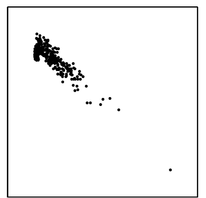
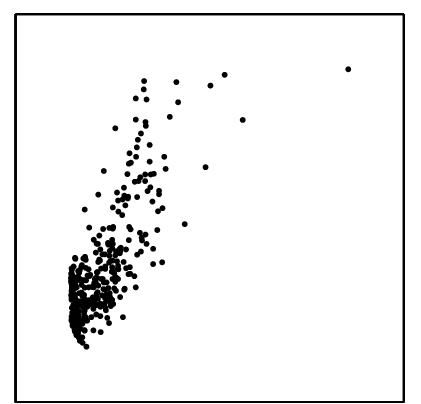
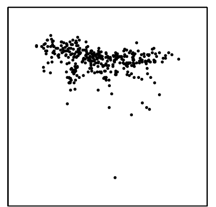
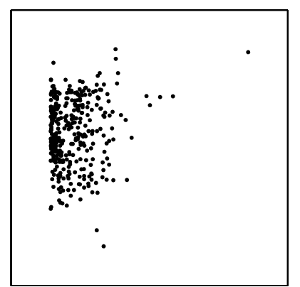
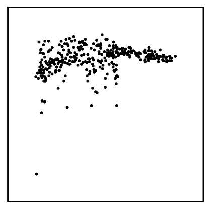
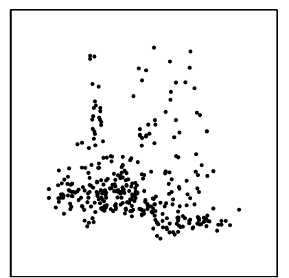
pair0001 pair0002 pair0003 pair0004 pair0020 pair0021

Figure 18: Scatter plots of pairs from D1. pair0001: altitude $\rightarrow$ temperature, pair0002: altitude $\rightarrow$ precipitation, pair0003: longitude $\rightarrow$ temperature, pair0004: altitude $\rightarrow$ sunshine hours, pair0020: latitude $\rightarrow$ temperature, pair0021: longitude $\rightarrow$ precipitation.

pair0001: Altitude $\rightarrow$ temperature

As an elementary fact of meteorology, places with higher altitude tend to be colder than those that are closer to sea level (roughly 1 centigrade per 100 meter). There is no doubt that altitude is the cause and temperature the effect: one could easily think of an intervention where the thermometer is lifted (e.g., by using a balloon) to measure the temperature at a higher point of the same longitude and latitude. On the other hand, heating or cooling a location usually does not change its altitude (except perhaps if the location happens to be the space enclosed by a hot air balloon, but let us assume that the thermometers used to gather this data were fixed to the ground). The altitudes in the DWD data set range from 0 m to 2960 m, which is sufficiently large to detect significant statistical dependences.

One potential confounder is latitude, since all mountains are in the south and far from the sea, which is also an important factor for the local climate. The places with the highest average temperatures are therefore those with low altitude but lying far in the south. Hence this confounder should induce positive correlations between altitude and temperature as opposed to the negative correlation between altitude and temperature that is observed empirically. This suggests that the direct causal relation between altitude and temperature dominates over the confounder.

pair0002: Altitude $\rightarrow$ precipitation

It is known that altitude is also an important factor for precipitation since rain often occurs when air is forced to rise over a mountain range and the air becomes oversaturated with water due to the lower temperature (orographic rainfall). This effect defines an indirect causal influence of altitude on precipitation via temperature. These causal relations are, however, less simple than the causal influence from altitude to temperature because gradients of the altitude with respect to the main direction of the wind are more relevant than the altitude itself. A hypothetical intervention that would allow us to validate the causal relation could be to build artificial mountains and observe orographic rainfall.

pair0003: Longitude $\rightarrow$ temperature

To detect the causal relation between longitude and temperature, a hypothetical intervention could be to move a thermometer between West and East. Even if one would adjust for altitude and latitude, it is unlikely that temperature would remain the same since the climate in the West is more oceanic and less continental than in the East of Germany. Therefore, longitude causes temperature.

pair0004: Altitude $\rightarrow$ sunshine hours

Sunshine duration and altitude are slightly positively correlated. Possible explanations are that higher weather stations are sometimes above low-hanging clouds. Cities in valleys, especially if they are close to rivers or lakes, typically have more misty days. Moving a sunshine sensor above the clouds clearly increases the sunshine duration whereas installing an artificial sun would not change the altitude. The causal influence from altitude to sunshine duration can be confounded, for instance, by the fact that there is a simple statistical dependence between altitude and longitude in Germany as explained earlier.

pair0020: Latitude $\rightarrow$ temperature

Moving a thermometer towards the equator will generally result in an increased mean annual temperature. Changing the temperature, on the other hand, does not necessarily result in a north-south movement of the thermometer. The obvious ground truth of latitude causing temperature might be somewhat “confounded” by longitude, in combination with the selection bias that arises from only including weather stations in Germany.

pair0021: Longitude $\rightarrow$ precipitation

As the climate in the West is more oceanic and less continental than in the East of Germany, we expect there to be a relationship between longitude and precipitation. Changing longitude by moving in East-West direction may therefore change precipitation, even if one would adjust for altitude and latitude. On the other hand, making it rain locally (e.g., by cloud seeding) will not result in a change in longitude.

D2: Abalone

The Abalone data set (Nash et al., 1994) in the UCI Machine Learning Repository (Bache and Lichman, 2013) contains 4177 measurements of several variables concerning the sea snail Abalone. We downloaded the data from https://archive.ics.uci.edu/ml/datasets/Abalone. The original data set contains the nine variables sex, length, diameter, height, whole weight, shucked weight, viscera weight, shell weight and number of rings. The number of rings in the shell is directly related to the age of the snail: adding 1.5 to the number of rings gives the age in years. Of these variables, we selected six pairs with obvious cause-effect relationships: age–length (pair0005), age–shell weight (pair0006), age–diameter (pair0007), age–height (pair0008), age–whole weight (pair0009), age–shucked weight (pair0010), age–viscera weight (pair0011).

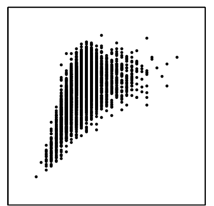
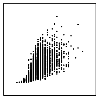
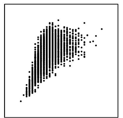
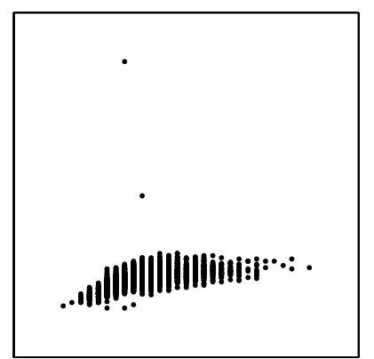
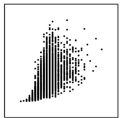
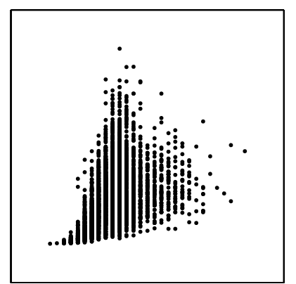
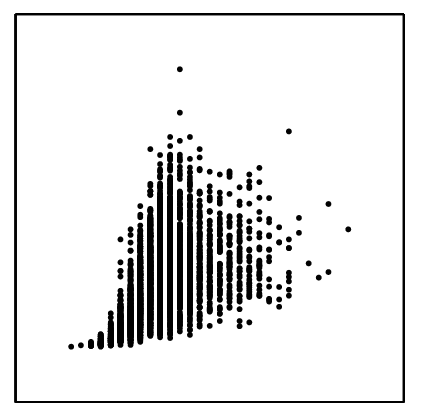
pair0005 pair0006 pair0007 pair0008 pair0009 pair0010 pair0011

Figure 19: Scatter plots of pairs from D2. pair0005: age $\rightarrow$ length, pair0006: age $\rightarrow$ shell weight, pair0007: age $\rightarrow$ diameter, pair0008: age $\rightarrow$ height, pair0009: age $\rightarrow$ whole weight, pair0010: age $\rightarrow$ shucked weight, pair0011: age $\rightarrow$ viscera weight.

pair0005–pair0011: Age $\rightarrow$ {length, shell weight, diameter, height, whole/shucked/viscera weight}

For the variable “age” it is not obvious what a reasonable intervention would be since there is no possibility to change the time. However, waiting and observing how variables change over time can be considered as equivalent to the hypothetical intervention on age (provided that the relevant background conditions do not change too much). Clearly, this “intervention” would change the probability distribution of the length, whereas changing the length of snails (by surgery) would not change the distribution of age (assuming that the surgery does not take years). Regardless of the difficulties of defining interventions, we expect common agreement on the ground truth: age causes all the other variables related to length, diameter height and weight.

There is one subtlety that has to do with how age is measured for these shells: this is done by counting the rings. For the variable “number of rings” however, changing the length of the snail may actually change the number of rings. We here presume that all snails have undergone their natural growing process so that the number of rings is a good proxy for the variable age.

D3: Census Income KDD

The Census Income (KDD) data set (U.S. Department of Commerce, 1994) in the UCI Machine Learning Repository (Bache and Lichman, 2013) has been extracted from the 1984 and 1985 U.S. Census studies. We downloaded the data from https://archive.ics.uci.edu/ml/datasets/Census-Income+(KDD). We have selected the following variables: AAGE (age), AHRSPAY (wage per hour) and DIVVAL (dividends from stocks).

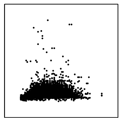
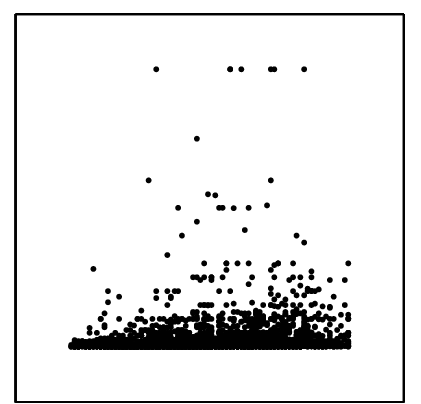
pair0012 pair0017

Figure 20: Scatter plots of pairs from D3. pair0012: age $\rightarrow$ wage per hour, pair0017: age $\rightarrow$ dividends from stocks.

pair0012: Age $\rightarrow$ wage per hour

We only used the first 5000 instances for which wage per hour was not equal to zero. The data clearly shows an increase of wage up to about 45 and a decrease for higher age.

As already argued for the Abalone data, interventions on the variable “age” are difficult to define. Compared to the discussion in the context of the Abalone data set, it seems more problematic to consider waiting as a reasonable “intervention” here, since the relevant (economical) background conditions change rapidly compared to the length of the human life: If someone’s salary is higher than the salary of a 20 year younger colleague because of his/her longer job experience, we cannot conclude that the younger colleague will earn the same money 20 years later as the older colleague earns now. Possibly, the factory or even the branch of industry he/she was working in does not exist any more and his/her job experience is no longer appreciated. However, we know that employees sometimes indeed do get a higher income because of their longer job experience. Pretending longer job experience by a fake certificate of employment would be a possible intervention. On the other hand, changing the wage per hour is an intervention that is easy to imagine (though difficult for us to perform) and this would certainly not change the age.

pair0017: Age $\rightarrow$ dividends from stocks

We only used the first 5000 instances for which dividends from stocks was not equal to zero. Similar considerations apply as for age vs. wage per hour. Doing an intervention on age is not practical, but companies could theoretically intervene on the dividends from stocks, and that would not result in a change of age, obviously. On the other hand, age influences income, and thereby over time, the amount of money that people can invest in stocks, and thereby, the amount of dividends they earn from stocks. This causal relation is a very indirect one, though, and the dependence between age and dividends from stock is less pronounced than that between age and wage per hour.

D4: Auto-MPG

The Auto-MPG data set in the UCI Machine Learning Repository (Bache and Lichman, 2013) concerns city-cycle fuel consumption in miles per gallon (MPG), i.e., the number of miles a car can drive on one gallon of gasoline, and contains several other attributes, like displacement, horsepower, weight, and acceleration. The original dataset comes from the StatLib library (Meyer and Vlachos, 2014) and was used in the 1983 American Statistical Association Exposition. We downloaded the data from http://archive.ics.uci.edu/ml/datasets/Auto+MPG and selected only instances without missing data, thereby obtaining 392 samples.

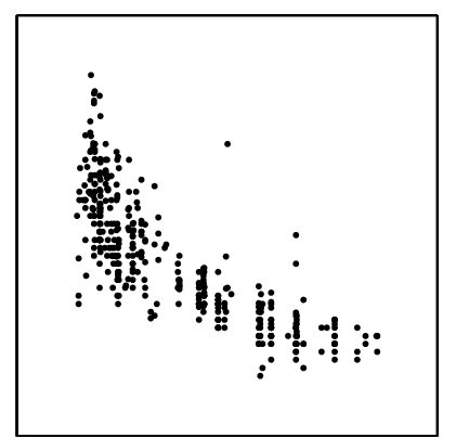
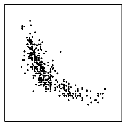
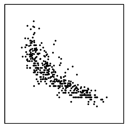
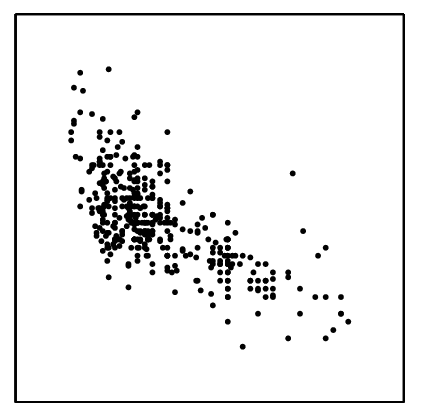
pair0013 pair0014 pair0015 pair0016

Figure 21: Scatter plots of pairs from D4. pair0013: displacement $\rightarrow$ fuel consumption, pair0014: horse power $\rightarrow$ fuel consumption, pair0015: weight $\rightarrow$ fuel consumption, pair0016: horsepower $\rightarrow$ acceleration, pair0054: (displacement,horsepower,weight) $\rightarrow$ (MPG,acceleration)

pair0013: Displacement $\rightarrow$ fuel consumption

Displacement is the total volume of air/fuel mixture an engine can draw in during one complete engine cycle. The larger the discplacement, the more fuel the engine can consume with every turn. Intervening on displacement (e.g., by increasing the cylinder bore) changes the fuel consumption. Changing the fuel consumption (e.g., by increasing the weight of the car, or changing its air resistance, or by using another gear) will not change the displacement, though.

pair0014: Horse power $\rightarrow$ fuel consumption

Horse power measures the amount of power an engine can deliver. There are various ways to define horsepower and different standards to measure horse power of vehicles. In general, though, it should be obvious that fuel consumption depends on various factors, including horse power. Changing horsepower (e.g., by adding more cylinders to an engine, or adding a second engine to the car) would lead to a change in fuel consumption. On the other hand, changing fuel consumption does not necessarily change horse power.

pair0015: Weight $\rightarrow$ fuel consumption

There is a strong selection bias here, as car designers use a more powerful motor (with higher fuel consumption) for a heavier car. Nevertheless, the causal relationship between weight and fuel consumption should be obvious: if we intervene on weight, then fuel consumption will change, but not necessarily vice versa.

pair0016: Horsepower $\rightarrow$ acceleration

Horsepower is one one of the factors that cause acceleration. Other factors are wheel size, the gear used, and air resistance. Intervening on acceleration does not necessarily change horsepower.

pair0054: (Displacement,horsepower,weight) $\rightarrow$ (MPG,acceleration)

This pair consists of two multivariate variables that are combinations of the variables we have considered before. The multivariate variable consisting of the three components displacement, horsepower and weight can be considered to cause the multivariate variable comprised of fuel consumption and acceleration.

D5: GAGurine

This data concerns the concentration of the chemical compound Glycosaminoglycan (GAG) in the urine of 314 children aged from zero to seventeen years. This is the GAGurine data set supplied with the MASS package of the computing language R (Venables and Ripley, 2002).

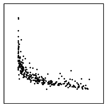
pair0018

Figure 22: Scatter plots of pairs from D5. pair0018: age $\rightarrow$ concentration GAG.

pair0018: Age $\rightarrow$ concentration GAG

Obviously, GAG concentration does not cause age, but it could be the other way around, considering the strong dependence between the two variables.

D6: Old Faithful

This is the geyser data set supplied with the MASS package of the computing language R (Venables and Ripley, 2002). It is originally described in (Azzalini and Bowman, 1990) and contains data about the duration of an eruption and the time interval between subsequent eruptions of the Old Faithful geyser in Yellowstone National Park, USA. The data consists of 194 samples and was collected in a single continuous measurement from August 1 to August 15, 1985.

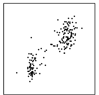
pair0019

Figure 23: Scatter plots of pairs from D6. pair0019: current duration $\rightarrow$ next interval.

pair0019: Current duration $\rightarrow$ next interval

The chronological ordering of events implicates that the time interval between the current and the next eruption is an effect of the duration of the current eruption.

D7: Arrhythmia

The Arrhythmia dataset (Guvenir et al., 1997) from the UCI Machine Learning Repository (Bache and Lichman, 2013) concerns cardiac arrhythmia. It consists of 452 patient records and contains many different variables. We downloaded the data from https://archive.ics.uci.edu/ml/datasets/Arrhythmia and only used the variables for which the causal relationships should be evident. We removed two instances from the dataset, corresponding with patient lengths of 680 and 780 cm, respectively.

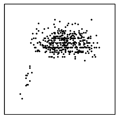
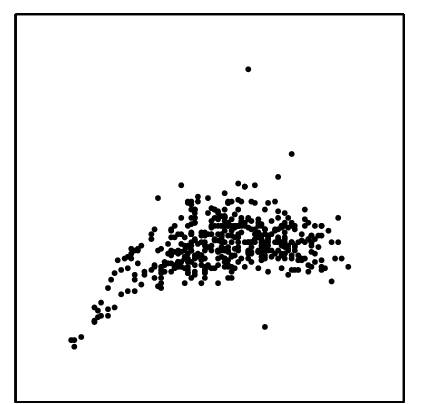
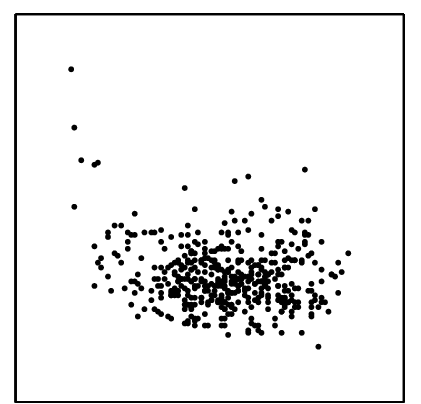
pair0022 pair0023 pair0024

Figure 24: Scatter plots of pairs from D7. pair0022: age $\rightarrow$ height, pair0023: age $\rightarrow$ weight, pair0024: age $\rightarrow$ heart rate.

pair0022–pair0024: Age $\rightarrow$ {height, weight, heart rate}

As discussed before, “interventions” on age (for example, waiting a few years) may affect height of persons. On the other hand, we know that height does not cause age. The same holds for age and weight and for age and heart rate. It is important to note here that age is simply measured in years since the birth of a person. Indeed, weight, height and also heart rate might influence “biological aging”, the gradual deterioration of function of the human body.

D8: Concrete Compressive Strength

This data set, available at the UCI Machine Learning Repository (Bache and Lichman, 2013), concerns a systematic study (Yeh, 1998) regarding concrete compressive strength as a function of ingredients and age. Citing (Yeh, 1998): “High-performance concrete (HPC) is a new terminology used in the concrete construction industry. In addition to the three basic ingredients in conventional concrete, i.e., Portland cement, fine and coarse aggregates, and water, the making of HPC needs to incorporate supplementary cementitious materials, such as fly ash and blast furnace slag, and chemical admixture, such as superplasticizer 1 and 2. Several studies independently have shown that concrete strength development is determined not only by the water-to-cement ratio, but that it also is influenced by the content of other concrete ingredients.” Compressive strength is measured in units of MPa, age in days, and the other variables are measured in kilograms per cubic metre of concrete mixture. The dataset was downloaded from https://archive.ics.uci.edu/ml/datasets/Concrete+Compressive+Strength and contains 1030 measurements.

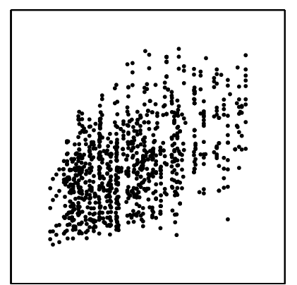
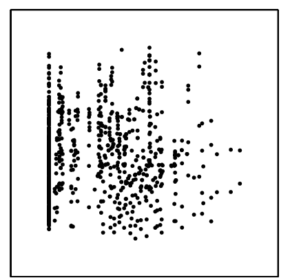
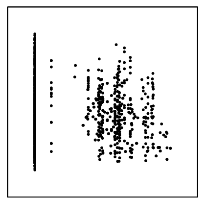
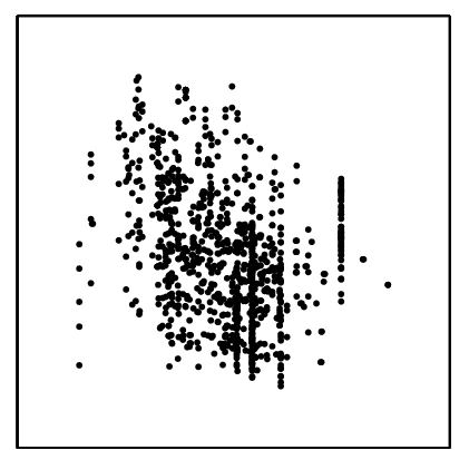
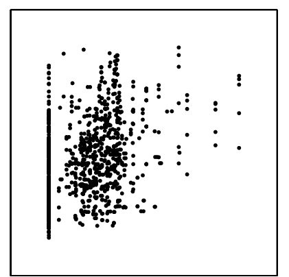
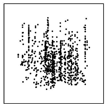
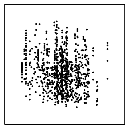
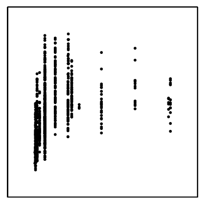
pair0025 pair0026 pair0027 pair0028 pair0029 pair0030 pair0031 pair0032

Figure 25: Scatter plots of pairs from D8. pair0025: cement $\rightarrow$ compressive strength, pair0026: blast furnace slag $\rightarrow$ compressive strength, pair0027: fly ash $\rightarrow$ compressive strength, pair0028: water $\rightarrow$ compressive strength, pair0029: superplasticizer $\rightarrow$ compressive strength, pair0030: coarse aggregate $\rightarrow$ compressive strength, pair0031: fine aggregate $\rightarrow$ compressive strength, pair0032: age $\rightarrow$ compressive strength.

pair0025–pair0032: {Cement, blast furnace slag, fly ash, water, superplasticizer, coarse aggregate, fine aggregate, age} $\rightarrow$ Compressive Strength

It should be obvious that compressive strength is the effect, and the other variables are its causes. Note, however, that in practice one cannot easily intervene on the mixture components without simultaneously changing the other mixture components. For example, if one adds more water to the mixture, then as a result, all other components will decrease, as they are measured in kilograms per cubic metre of concrete mixture. Nevertheless, we expect that we can see these interventions as reasonable approximations of “perfect interventions” on a single variable.

D9: Liver Disorders

This data set, available at the UCI Machine Learning Repository (Bache and Lichman, 2013), was collected by BUPA Medical Research Ltd. It consists of several blood test results, which are all thought to be indicative for liver disorders that may arise from excessive alcohol consumption. Each of the 345 instances constitutes the record of a single male individual. Daily alcohol consumption is measured in number of half-pint equivalents of alcoholic beverages drunk per day. The blood test results are mean corpuscular volume (MCV), alkaline phosphotase (ALP), alanine aminotransferase (ALT), aspartate aminotransferase (AST), and gamma-glutamyl transpeptidase (GGT). The data is available at https://archive.ics.uci.edu/ml/datasets/Liver+Disorders.

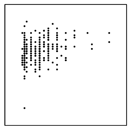
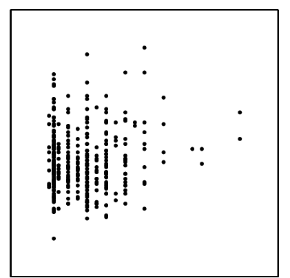
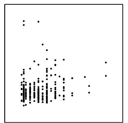
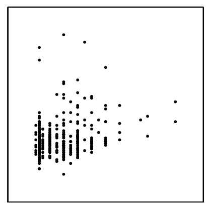
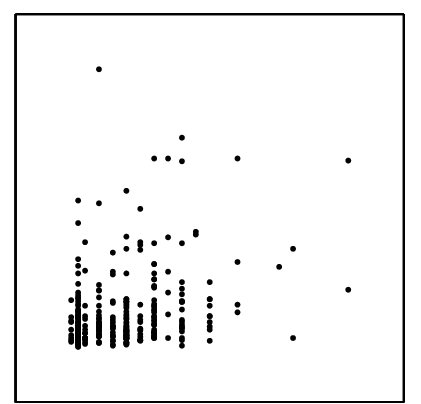
pair0033 pair0034 pair0035 pair0036 pair0037

Figure 26: Scatter plots of pairs from D9. pair0033: alcohol consumption $\rightarrow$ mean corpuscular volume, pair0034: alcohol consumption $\rightarrow$ alkaline phosphotase, pair0035: alcohol consumption $\rightarrow$ alanine aminotransferase, pair0036: alcohol consumption $\rightarrow$ aspartate aminotransferase, pair0037: alcohol consumption $\rightarrow$ gamma-glutamyl transpeptidase.

Although one would expect that daily alcohol consumption is the cause, and the blood test results are the effects, this is not necessarily the case. Indeed, citing (Baynes and Dominiczak, 1999): “[…] increased plasma concentrations of acetaldehyde after the ingestion of alcohol […] causes the individual to experience unpleasant flushing and sweating, which discourages alcohol abuse. Disulfiram, a drug that inhibits ALDH, also leads to these symptoms when alcohol is taken, and may be given to reinforce abstinence from alcohol.” This means that a priori, a reverse causation of the chemical whose concentration is measured in one of these blood tests on daily alcohol consumption cannot be excluded with certainty. Nevertheless, we consider this to be unlikely, as the medical literature describes how these particular blood tests can be used to diagnose liver disorders, but we did not find any evidence that these chemicals can be used to treat excessive alcohol consumption.

pair0033: Alcohol Consumption $\rightarrow$ Mean Corpuscular Volume

The mean corpuscular volume (MCV) is the average volume of a red blood cell. An elevated MCV has been associated with alcoholism (Tønnesen et al., 1986), but there are many other factors also associated with MCV.

pair0034: Alcohol Consumption $\rightarrow$ Alkaline Phosphotase

Alkaline phosphatase (ALP) is an enzyme that is predominantly abundant in liver cells, but is also present in bone and placental tissue. Elevated ALP levels in blood can be due to many different liver diseases and also bone diseases, but also occur during pregnancy (Braunwald et al., 2001).

pair0035: Alcohol Consumption $\rightarrow$ Alanine Aminotransferase

Alanine Aminotransferase (ALT) is an enzyme that is found primarily in the liver cells. It is released into the blood in greater amounts when there is damage to the liver cells, for example due to a viral hepatitis or bile duct problems. ALT levels are often normal in alcoholic liver disease (Braunwald et al., 2001).

pair0036: Alcohol Consumption $\rightarrow$ Aspartate Aminotransferase

Aspartate aminotransferase (AST) is an enzyme that is found in the liver, but also in many other bodily tissues, for example the heart and skeletal muscles. Similar to ALT, the AST levels raise in acute liver damage. Elevated AST levels are not specific to the liver, but can also be caused by other diseases, for example by pancreatitis. An AST:ALT ratio of more than 3:1 is highly suggestive of alcoholic liver disease (Braunwald et al., 2001).

pair0037: Alcohol Consumption $\rightarrow$ Gamma-Glutamyl Transpeptidase

Gamma-Glutamyl Transpeptidase (GGT) GGT is another enzyme that is primarily found in liver cells. It is rarely elevated in conditions other than liver disease. High GGT levels have been associated with alcohol use (Braunwald et al., 2001).

D10: Pima Indians Diabetes

This data set, available at the UCI Machine Learning Repository (Bache and Lichman, 2013), was collected by the National Institute of Diabetes and Digestive and Kidney Diseases in the USA to forecast the onset of diabetes mellitus in a high risk population of Pima Indians near Phoenix, Arizona. Cases in this data set were selected according to several criteria, in particular being female, at least 21 years of age and of Pima Indian heritage. This means that there could be selection bias on age.

We downloaded the data from https://archive.ics.uci.edu/ml/datasets/Pima+Indians+Diabetes. We only selected the instances with nonzero values, as it seems likely that zero values encode missing data. This yielded 768 samples.

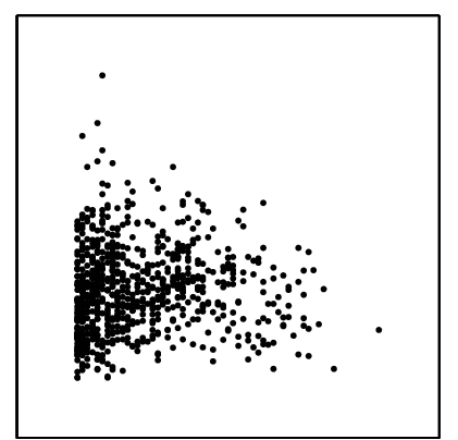
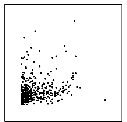
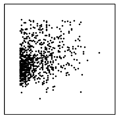
pair0038 pair0039 pair0040 pair0041

Figure 27: Scatter plots of pairs from D10. pair0038: age $\rightarrow$ body mass index, pair0039: age $\rightarrow$ serum insulin, pair0040: age $\rightarrow$ diastolic blood pressure, pair0041: age $\rightarrow$ plasma glucose concentration.

pair0038: Age $\rightarrow$ Body Mass Index

Body mass index (BMI) is defined as the ratio between weight (kg) and the square of height (m). Obviously, age is not caused by body mass index, but as age is a cause of both height and weight, age causes BMI.

pair0039: Age $\rightarrow$ Serum Insulin

2-Hour serum insulin ($\mu$U/ml), measured 2 hours after the ingestion of a standard dose of glucose, in an oral glucose tolerance test. We can exclude that serum insulin causes age, and there could be an effect of age on serum insulin. Another explanation for the observed dependence could be the selection bias.

pair0040: Age $\rightarrow$ Diastolic Blood Pressure

Diastolic blood pressure (mm Hg). It seems obvious that blood pressure does not cause age. The other causal direction seems plausible, but again, an alternative explanation for the dependence could be selection bias.

pair0041: Age $\rightarrow$ Plasma Glucose Concentration

Plasma glucose concentration, measured 2 hours after the ingestion of a standard dose of glucose, in an oral glucose tolerance test. Similar reasoning as before: we do not believe that plasma glucose concentration causes ages, but it could be the other way around, and there may be selection bias.

D11: B. Janzing’s meteo data

This data set is from a private weather station, owned by Bernward Janzing, located in Furtwangen (Black Forest), Germany at an altitude of 956 m. The measurements include temperature, precipitation, and snow height (since 1979), as well as solar radiation (since 1986). The data have been archived by Bernward Janzing, statistical evaluations have been published in (Janzing, 2004), monthly summaries of the weather are published in local newspapers since 1981.

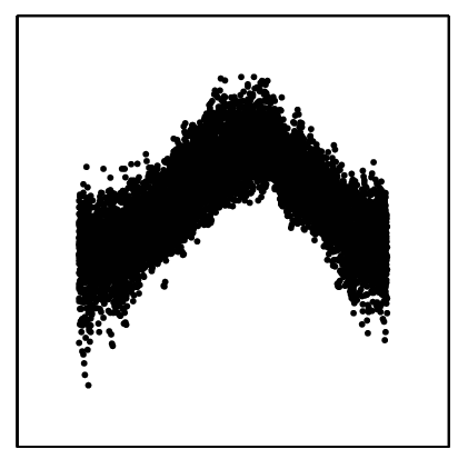
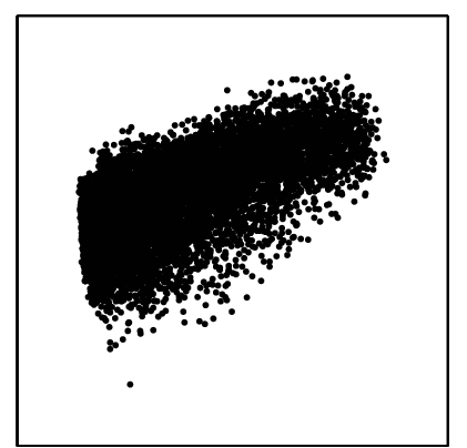
pair0042 pair0077

Figure 28: Scatter plots of pairs from D11. pair0042: day of the year $\rightarrow$ temperature, pair0077: solar radiation $\rightarrow$ temperature.

pair0042: Day of the year $\rightarrow$ Temperature

This data set shows the dependence between season and temperature over 25 years plus one month, namely the time range 01/01/1979–01/31/2004. It consists of 9162 measurements.

One variable is the day of the year, represented by an integer from $1$ to $365$ (or $366$ for leap years). The information about the year has been dropped. $Y$ is the mean temperature of the respective day, calculated according to the following definition:

$$T_{mean}:=\frac{T_{morning}+T_{midday}+2T_{evening}}{4},$$

where morning, midday, and evening are measured at 7:00 am, 14:00 pm, and 21:00 pm (MEZ), respectivley (without daylight saving time). Double counting of the evening value is official standard of the German authority “Deutscher Wetterdienst”. It has been defined at a time where no electronic data loggers were available and thermometers had to be read out by humans. Weighting the evening value twice has been considered a useful heuristics to account for the missing values at night.

We consider day of the year as the cause, since it can be seen as expressing the angular position on its orbit around the sun. Although true interventions are infeasible, it is commonly agreed that changing the position of the earth would result in temperature changes at a fixed location due to the different solar incidence angle.

pair0077: Solar radiation $\rightarrow$ Temperature

This data set shows the relation between solar radiation and temperature over 23 years, namely the interval 01/01/1986–12/31/2008. It consists of 8401 measurements.

Solar radiation is measured per area in $\mathrm{W}/\mathrm{m}^{2}$ averaged over one day on a horizontal surface. Temperature is the averaged daily, as in pair0042. The original data has been processed by us to extract the common time interval. We assume that radiation causes temperature. High solar radiation increases the temperature of the air already at a scale of hours. Interventions are easy to implement: Creating artificial shade on a large enough surface would decrease the air temperature. On longer time scales there might also be an influence from temperature to radiation via the generation of clouds through evaporation in more humid environments. This should, however, not play a role for daily averages.

D12: NCEP-NCAR Reanalysis

This data set, available from the NOAA (National Oceanic and Atmospheric Administration) Earth System Research Laboratory website at http://www.esrl.noaa.gov/psd/data/gridded/data.ncep.reanalysis.surface.html, is a subset of a reanalysis data set, incorporating observations and numerical weather prediction model output from 1948 to date (Kalnay et al., 1996). The reanalysis data set was produced by the National Center for Environmental Prediction (NCEP) and the National Center for Atmospheric Research (NCAR). Reanalysis data products aim for a realistic representation of all relevant climatological variables on a spatiotemporal grid. We collected four variables from a global grid of 144 $\times$ 73 cells: air temperature (in K, pair0043), surface pressure (in Pascal, pair0044), sea level pressure (in Pascal, pair0045) and relative humidity (in $\%$, pair0045) on two consecutive days, day 50 and day 51 of the year 2000 (i.e., Feb 19th and 20th). Each data pair consists of $144\times 73-143=10369$ data points, distributed across the globe. 143 data points were subtracted because at the north pole values are repeated across all longitudes.

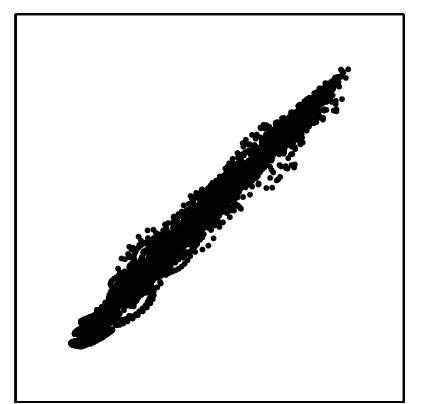
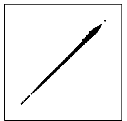
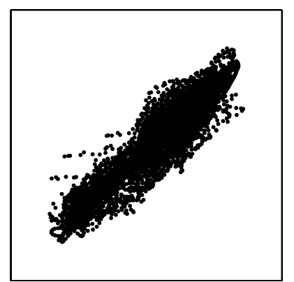
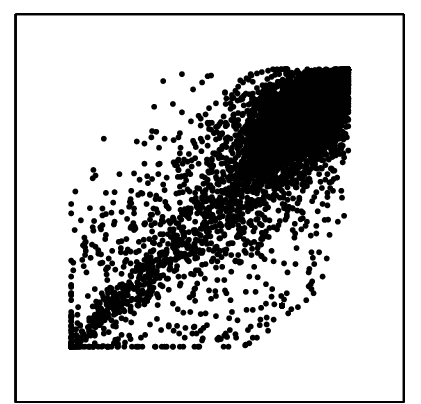
pair0043 pair0044 pair0045 pair0046

Figure 29: Scatter plots of pairs from D12. pair0043: temperature at t $\rightarrow$ temperature at t+1, pair0044: surface oressure at t $\rightarrow$ surface pressure at t+1, pair0045: sea level oressure at t $\rightarrow$ sea level pressure at t+1, pair0046: relative humidity at t $\rightarrow$ relative humidity at t+1, pair0052: (temp, press, slp, rh) at t $\rightarrow$ (temp, press, slp, rh) at t+1.

Each data point is the daily average over an area that covers 2.5^∘ $\times$ 2.5^∘ (approximately 250 km $\times$ 250 km at the equator). Because causal influence cannot propagate backwards in time, temperature, pressure and humidity in a certain area are partly affected by their value the day before in the same area.

pair0043: Temperature at t $\rightarrow$ Temperature at t+1

Due to heat storage, mean daily air temperature near surface at any day largely impact daily air temperature at the following day. We assume there is no causation backwards in time, hence the correlation between temperatures at two consecutive days must be driven by confounders (such as large-scale weather patterns) or a causal influence from the first day to the second.

pair0044: Surface Pressure at t $\rightarrow$ Surface Pressure at t+1

Pressure patterns near the earth’s surface are mostly driven by large-scale weather patterns. However, large-scale weather patterns are also driven by local pressure gradients and hence, some of the correlation between surface pressure at two consecutive days stems from a direct causal link between the first and the second day, as we assume there is no causation in time.

pair0045: Sea Level Pressure at t $\rightarrow$ Sea Level Pressure at t+1

Similar reasoning as in pair0044.

pair0046: Relative Humidity at t $\rightarrow$ Relative Humidity at t+1

Humidity of the air at one day affects the humidity of the following day because if no air movement takes place and no drying or moistening occurs, it will approximately stay the same. Furthermore, as reasoned above, because there is no causation backwards in time, relative humidity at day $t+1$ cannot affect humidity at day $t$. Note that relative humidity has values between 0 and 100. Values can be saturated in very humid places such as tropical rainforest and approach 0 in deserts. For this reason, the scatter plot looks as if the data were clipped.

pair0052: (Temp, Press, SLP, RH) at t $\rightarrow$ (Temp, Press, SLP, RH) at t+1

The pairs pair0043–pair0046 were combined to a 4-dimensional vector. From the reasoning above it follows that the vector of temperature, near surface pressure, sea level pressure and relative humidity at day $t$ has a causal influence on the vector of the same variables at time $t+1$.

D13: Traffic

This dataset has been extracted from http://www.b30-oberschwaben.de/html/tabelle.html, a website containing various kinds of information about the national highway B30. This is a road in the federal state Baden-Württemberg, Germany, which provides an important connection of the region around Ulm (in the North) with the Lake Constance region (in the South). After extraction, the data set contains 254 samples.

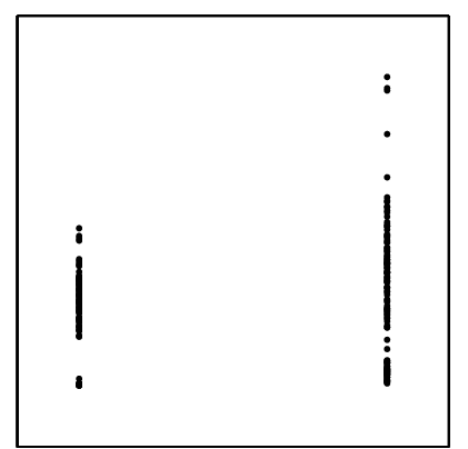
pair0047

Figure 30: Scatter plots of pairs from D13. pair0047: type of day $\rightarrow$ number of cars.

pair0047: Type of Day $\rightarrow$ Number of Cars

One variable is the number of cars per day, the other denotes the type of the respective day, with “1” indicating Sundays and holidays and “2” indicating working days. The type of day causes the number of cars per day. Indeed, introducing an additional holiday by a political decision would certainly change the amount of traffic on that day, while changing the amount of traffic by instructing a large number of drivers to drive or not to drive at a certain day would certainly not change the type of that day.

D14: Hipel & McLeod

This dataset contains 168 measurements of indoor and outdoor temperatures. It was taken from a book by Hipel and McLeod (1994) and can be downloaded from http://www.stats.uwo.ca/faculty/mcleod/epubs/mhsets/readme-mhsets.html.

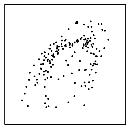
pair0048

Figure 31: Scatter plots of pairs from D14. pair0048: outdoor temperature $\rightarrow$ indoor temperature.

pair0048: Outdoor temperature $\rightarrow$ Indoor temperature

Outdoor temperatures can have a strong impact on indoor temperatures, in particular when indoor temperatures are not adjusted by air conditioning or heating. Contrarily, indoor temperatures will have little or no effect on outdoor temperatures, because the outside environment has a much larger heat capacity.

D15: Bafu

This data set deals with the relationship between daily ozone concentration in the air and temperature. It was downloaded from http://www.bafu.admin.ch/luft/luftbelastung/blick_zurueck/datenabfrage/index.html. Lower atmosphere ozone (O₃) is a secondary pollutant that is produced by the photochemical oxidation of carbon monoxide (CO), methane (CH₄), and non-methane volatile organic compounds (NMVOCs) by OH in the presence of nitrogen oxides (NO_x, NO + NO₂) (Rasmussen et al., 2012). It is known that ozone concentration strongly correlates with surface temperature (Bloomer et al., 2009). Several explanations are given in the literature (see e.g., Rasmussen et al., 2012). Without going into details of the complex underlying chemical processes, we mention that the crucial chemical reactions are stronger at higher temperatures. For instance, isoprene emissions of plants increase with increasing temperature and isoprene can play a similar role in the generation of O₃ as NO_x (Rasmussen et al., 2012). Apart from this, air pollution may be influenced indirectly by temperature, e.g., via increasing traffic at ‘good’ weather conditions or an increased occurrence rate of wildfires. All these explanations state a causal path from temperature to ozone. Note that the phenomenon of ozone pollution in the lower atmosphere discussed here should not be confused with the ‘ozone hole’, which is a lack of ozone in the higher atmosphere. Close to the surface, ozone concentration does not have an impact on temperatures. For all three data sets, ozone is measured in $\mu$g/m³ and temperature in ^∘C.

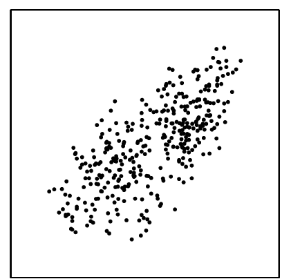
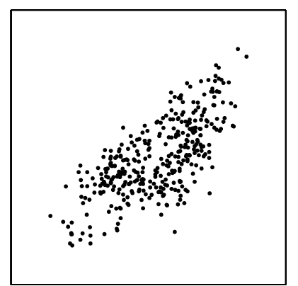
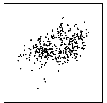
pair0049 pair0050 pair0051

Figure 32: Scatter plots of pairs from D15. pair0049: temperature $\rightarrow$ ozone concentration, pair0050: temperature $\rightarrow$ ozone concentration, pair0051: temperature $\rightarrow$ ozone concentration, pair0055: radiation $\rightarrow$ ozone concentration.

pair0049: Temperature $\rightarrow$ Ozone concentration

365 daily mean values of ozone and temperature of year 2009 in Lausanne-César-Roux, Switzerland.

pair0050: Temperature $\rightarrow$ Ozone concentration

365 daily mean values of ozone and temperature of year 2009 in Chaumont, Switzerland.

pair0051: Temperature $\rightarrow$ Ozone concentration

365 daily mean values of ozone and temperature of year 2009 in Davos-See, Switzerland.

pair0055: Radiation $\rightarrow$ Ozone concentration

72 daily mean values of ozone concentrations and radiation in the last 83 days of 2009 at 16 different places in Switzerland (11 days were deleted due to missing data). Solar radiation and surface ozone concentration are correlated (Feister and Balzer, 1991). The deposition of ozone is driven by complex micrometeorological processes including wind direction, air temperature, and global radiation (Stockwell et al., 1997). For instance, solar radiation affects the height of the planetary boundary layer and cloud formation and thus indirectly influences ozone concentrations. In contrast, global radiation is not driven by ozone concentrations close to the surface.

Ozone is given in $\mu$g/m³, radiation in W/m². The 16 different places are: 1: Bern-Bollwerk, 2: Magadino-Cadenazzo, 3: Lausanne-César-Roux, 4: Payerne, 5: Lugano-Universita, 6: Taenikon, 7: Zuerich-Kaserne, 8: Laegeren, 9: Basel-Binningen, 10: Chaumont, 11: Duebendorf, 12: Rigi-Seebodenalp, 13: Haerkingen, 14: Davos-See, 15: Sion-Aéroport, 16: Jungfraujoch.

D16: Environmental

We downloaded ozone concentration, wind speed, radiation and temperature from http://www.mathe.tu-freiberg.de/Stoyan/umwdat.html, discussed in Stoyan et al. (1997). The data consist of 989 daily values over the time period from 05/01/1989 to 10/31/1994 observed in Heilbronn, Germany.

pair0053: (wind speed, radiation, temperature) $\rightarrow$ Ozone concentration

As we have argued above in Section D15, wind direction (and speed), air temperature, and global radiation influence local ozone concentrations. Wind can influence ozone concentrations for example in the following way. No wind will keep the the concentration of ozone in a given air parcel constant if no lateral or vertical sources or sinks are prevalent. In contrast, winds can move and disperse and hence mix air with different ozone concentrations. Ozone concentration is given in $\mu$g/m³, wind speed in m/s, global radiation in W/m² and temperature in ^∘C.

D17: UNdata

The following data were taken from the “UNdata” database of the United Nations Statistics Division at http://data.un.org.

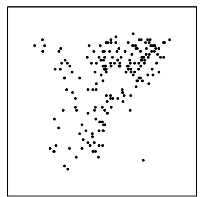
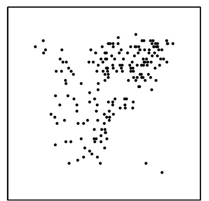
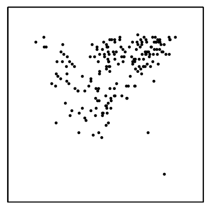
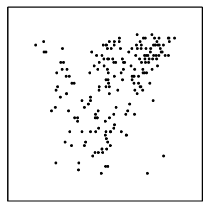
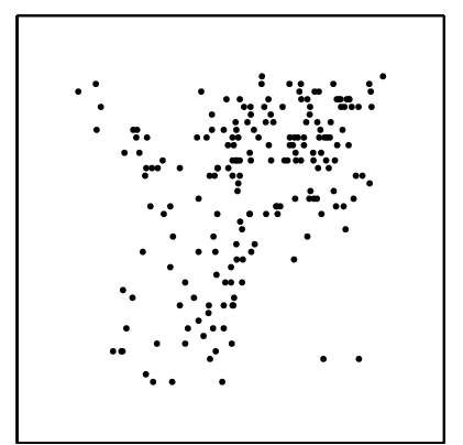
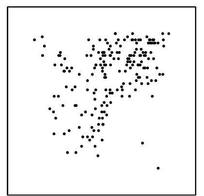
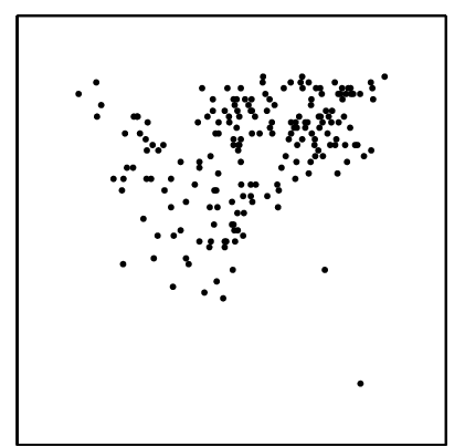
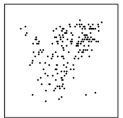
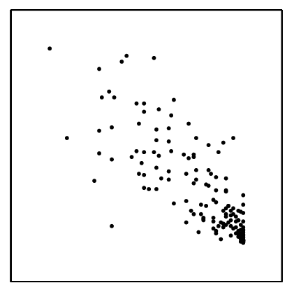
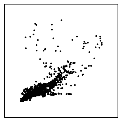
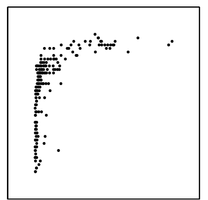
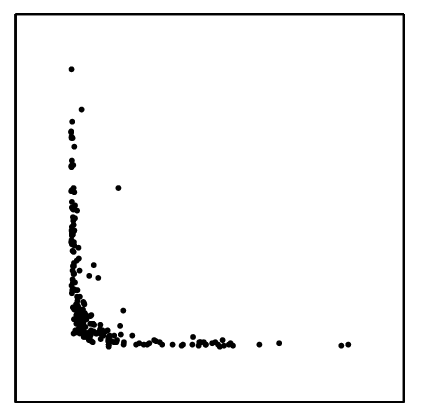
pair0056 pair0057 pair0058 pair0059 pair0060 pair0061 pair0062 pair0063 pair0064 pair0073 pair0074 pair0075

Figure 33: Scatter plots of pairs from D17. pair0056–pair0059: latitude of capital $\rightarrow$ female life expectancy, pair0060–pair0063: latitude of capital $\rightarrow$ male life expectancy, pair0064: drinking water access $\rightarrow$ infant mortality, pair0073: energy use $\rightarrow$ CO₂ emissions, pair0074: GNI per capita $\rightarrow$ life expectancy, pair0075: GNI per capita $\rightarrow$ under-5 mortality rate.

pair0056–pair0059: Latitude of Capital $\rightarrow$ Female Life Expectancy

Pairs pair0056–pair0059 consist of female life expectancy (in years) at birth versus latitude of the country’s capital, for various countries (China, Russia and Canada were removed). The four pairs correspond with measurements over the periods 2000–2005, 1995–2000, 1990–1995, 1985–1990, respectively. The data were downloaded from http://data.un.org/Data.aspx?d=GenderStat&f=inID%3a37.

The location of a country (encoded in the latitude of its capital) has an influence on how poor or rich a country is, hence affecting the quality of the health care system and ultimately life expectancy. This influence could stem from abundance of natural resources within the country’s borders or the influence neighboring countries have on its economic welfare. Furthermore, the latitude can influence life expectancy via climatic factors. For instance, life expectancy might be smaller if a country frequently experiences climatic extremes. In contrast, it is clear that life expectancy does not have any effect on latitude.

pair0060–pair0063: Latitude of Capital $\rightarrow$ Male Life Expectancy

Pairs pair0060–pair0063 are similar, but concern male life expectancy. The same reasoning as for female life expectancy applies here.

pair0064: Drinking Water Access $\rightarrow$ Infant Mortality

Here, one variable describes the percentage of population with sustainable access to improved drinking water sources in 2006, whereas the other variable denotes the infant mortality rate (per 1000 live births) for both sexes. The data were downloaded from http://data.un.org/Data.aspx?d=WHO&f=inID%3aMBD10 and http://data.un.org/Data.aspx?d=WHO&f=inID%3aRF03, respectively, and consist of 163 samples.

Clean drinking water is a primary requirement for health, in particular for infants (Esrey et al., 1991). Changing the percentage of people with access to clean water will directly change the mortality rate of infants, since infants are particularly susceptible to diseases (Lee et al., 1997). There may be some feedback, because if infant mortality is high in a poor country, development aid may be directed towards increasing the access to clean drinking water.

pair0073: Energy Use $\rightarrow$ CO₂ Emissions

This data set contains energy use (in kg of oil equivalent per capita) and CO₂ emission data from 152 countries between 1960 and 2005, yielding together 5084 samples. Considering the current energy mix across the world, the use of energy clearly results in CO₂ emissions (although in varying amounts across energy sources). Contrarily, a hypothetical change in CO₂ emissions will not affect the energy use of a country on the short term. On the longer term, if CO₂ emissions increase, this may cause energy use to decrease because of fear for climate change.

pair0074: GNI per capita $\rightarrow$ Life Expectancy

We collected the Gross National Income (GNI, in USD) per capita and the life expectancy at birth (in years) for 194 different countries. GNI can be seen as an index of wealth of a country. In general, richer countries have a better health care system than poor countries an thus can take better care of their citizens when they are ill. Reversely, we believe that the life expectancy of humans has a smaller impact on how wealthy a country is than vice versa.

pair0075: GNI per capita $\rightarrow$ Under-5 Mortality Rate

Here we collected the Gross National Income (GNI, in USD) per capita and the under-5 mortality rate (deaths per 1000 live births) for 205 different countries. The reasoning is similar as in pair0074. GNI as an index of wealth influences the quality of the health care system, which in turn determines whether young children will or will not die from minor diseases. As children typically do not contribute much to GNI per capita, we do not expect the reverse causal relation to be very strong.

D18: Yahoo database

These data denote stock return values and were downloaded from http://finance.yahoo.com. We collected 1331 samples from the following stocks between January 4th, 2000 and June 17, 2005: Hang Seng Bank (0011.HK), HSBC Hldgs (0005.HK), Hutchison (0013.HK), Cheung kong (0001.HK), and Sun Hung Kai Prop. (0016.HK). Subsequently, the following preprocessing was applied, which is common in financial data processing:

1. Extract the dividend/split adjusted closing price data from the Yahoo Finance data base.

2. For the few days when the price is not available, we use simple linear interpolation to estimate the price.

3. For each stock, denote the closing price on day $t$ by $P_{t}$, and the corresponding return is calculated as $X_{t}=(P_{t}-P_{t-1})/P_{t-1}$.

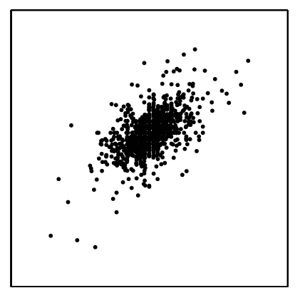
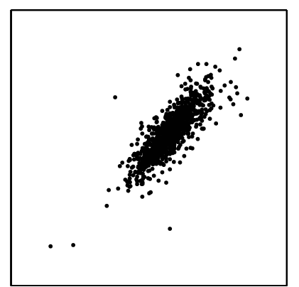
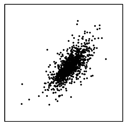
pair0065 pair0066 pair0067

Figure 34: Scatter plots of pairs from D18. pair0065: Stock Return of Hang Seng Bank $\rightarrow$ Stock Return of HSBC Hldgs, pair0066: Stock Return of Hutchison $\rightarrow$ Stock Return of Cheung kong, pair0067: Stock Return of Cheung kong $\rightarrow$ Stock Return of Sun Hung Kai Prop.

pair0065: Stock Return of Hang Seng Bank $\rightarrow$ Stock Return of HSBC Hldgs

HSBC owns 60$\%$ of Hang Seng Bank. Consequently, if stock returns of Hang Seng Bank change, this should have an influence on stock returns of HSBC Hldgs, whereas causation in the other direction would be expected to be less strong.

pair0066: Stock Return of Hutchison $\rightarrow$ Stock Return of Cheung kong

Cheung kong owns about 50$\%$ of Hutchison. Same reasoning as in pair0065.

pair0067: Stock Return of Cheung kong $\rightarrow$ Stock Return of Sun Hung Kai Prop.

Sun Hung Kai Prop. is a typical stock in the Hang Seng Property subindex, and is believed to depend on other major stocks, including Cheung kong.

D19: Internet traffic data

This dataset has been created from the log-files of a http-server of the Max Planck Institute for Intelligent Systems in Tübingen, Germany. The variable Internet connections counts the number of times an internal website of the institute has been accessed during a time interval of $1$ minute (more precisely, it counts the number of URL requests). Requests for non-existing websites are not counted. The variable Byte transferred counts the total number of bytes sent for all those accesses during the same time interval. The values $(x_{1},y_{1}),\dots,(x_{498},y_{498})$ refer to $498$ time intervals. To avoid too strong dependence between the measurements, the time intervals are not adjacent but have a distance of $20$ minutes.

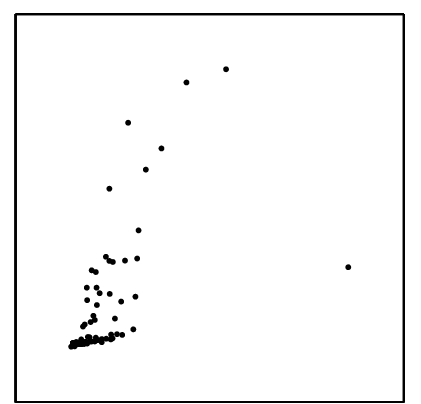
pair0068

Figure 35: Scatter plots of pairs from D19. pair0068: internet connections $\rightarrow$ bytes transferred.

pair0068: Internet connections $\rightarrow$ Bytes transferred

Internet connections causes Bytes transferred because an additional access of the website raises the transfer of data, while transferring more data does not create an additional website access. Note that not every access yields data transfer because the website may still be cached. However, this fact does not spoil the causal relation, it only makes it less deterministic.

D20: Inside and outside temperature

This bivariate time-series data consists of measurements of inside room temperature (^∘C) and outside temperature (^∘C), where measurements were taken every 5 minutes for a period of about 56 days, yielding a total of 16382 measurements. The outside thermometer was located on a spot that was exposed to direct sunlight, which explains the large fluctuations. The data were collected by Joris M. Mooij.

pair0069

Figure 36: Scatter plots of pairs from D20. pair0069: outside temperature $\rightarrow$ inside temperature.

pair0069: Outside Temperature $\rightarrow$ Inside Temperature

Although there is a causal relationship in both directions, we expect that the strongest effect is from outside temperature on inside temperature, as the heat capacity of the inside of a house is much smaller than that of its surroundings. See also the reasoning for pair0048.

D21: Armann & Buelthoff’s data

This dataset is taken from a psychological experiment that artificially generates images of human faces that interpolate between male and female, taking real faces as basis (Armann and Bülthoff, 2012). The interpolation is done via principal component analysis after representing true face images as vectors in an appropriate high-dimensional space. Human subjects are instructed to label the faces as male or female. The variable “parameter” runs between $0$ and $14$ and describes the transition from female to male. It is chosen by the experimenter. The binary variable “answer” indicates the answers ‘female’ and ’male’, respectively. The dataset consists of 4499 samples.

pair0070

Figure 37: Scatter plots of pairs from D21. pair0070: parameter $\rightarrow$ answer.

pair0070: Parameter $\rightarrow$ Answer

Certainly parameter causes answer. We do not have to talk about hypothetical interventions. Instead, we have a true intervention, since “parameter” has been set by the experimenter.

D22: Acute Inflammations

This data set, available at the UCI Machine Learning Repository (Bache and Lichman, 2013), was collected in order to create a computer expert system that decides whether a patient suffers from two different diseases of urinary system (Czerniak and Zarzycki, 2003). We downloaded it from https://archive.ics.uci.edu/ml/datasets/Acute+Inflammations. The two possible diseases are acute inflammations of urinary bladder and acute nephritises of renal pelvis origin. As it is also possible to chose none of those, the class variable takes values in $\{0,1\}^{2}$. The decision is based on six symptoms: temperature of patient (e.g. $35.9$), occurrence of nausea (“yes” or “no”), lumbar pain (“yes” or “no”), urine pushing (“yes” or “no”), micturition pains (“yes” or “no”) and burning of urethra, itch, swelling of urethra outlet (“yes” or “no”). These are grouped together in a six-dimensional vector “symptoms”.

pair0071: Symptoms $\rightarrow$ classification of disease

One would think that the disease is causing the symptoms but this data set was created artificially. The description on the UCI homepage says: “The data was created by a medical expert as a data set to test the expert system, which will perform the presumptive diagnosis of two diseases of urinary system. (…) Each instance represents an potential patient.” We thus consider the symptoms as the cause for the expert’s decision.

D23: Sunspot data

The data set consists of 1632 monthly values between May 1874 and April 2010 and therefore contains $1632$ data points. The temperature data have been taken from http://www.cru.uea.ac.uk/cru/data/temperature/ and have been collected by Climatic Research Unit (University of East Anglia) in conjunction with the Hadley Centre (at the UK Met Office) (Morice et al., 2012). The temperature data is expressed in deviations from the 1961–90 mean global temperature of the Earth (i.e., monthly anomalies). The sunspot data (Hathaway, 2010) are taken from the National Aeronautics and Space Administration and were downloaded from http://solarscience.msfc.nasa.gov/SunspotCycle.shtml. According to the description on that website, “sunspot number is calculated by first counting the number of sunspot groups and then the number of individual sunspots. The sunspot number is then given by the sum of the number of individual sunspots and ten times the number of groups. Since most sunspot groups have, on average, about ten spots, this formula for counting sunspots gives reliable numbers even when the observing conditions are less than ideal and small spots are hard to see.”

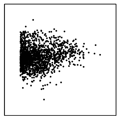
pair0072

Figure 38: Scatter plots of pairs from D23. pair0072: sunspots $\rightarrow$ global mean temperature.

pair0072: Sunspots $\rightarrow$ Global Mean Temperature

Sunspots are phenomena that appear temporarily on the sun’s surface. Although the causes of sunspots are not entirely understood, there is a significant dependence between the number of sunspots and the global mean temperature anomalies ($p$-value for zero correlation is less than $10^{-4}$). There is evidence that the Earth’s climate heats and cools as solar activity rises and falls (Haigh, 2007), and the sunspot number can be seen as a proxy for solar activity. Also, we do not believe that the Earth’s surface temperature (or changes of the Earth’s atmosphere) has an influence on the activity of the sun. We therefore consider number of sunspots causing temperature as the ground truth.

D24: Food and Agriculture Organization of the UN

The data set has been collected by Food and Agriculture Organization of the UN (http://www.fao.org/economic/ess/ess-fs/en/) and is accessible at http://www.docstoc.com/docs/102679223/Food-consumption-and-population-growth---FAO. It covers $174$ countries or areas during the period from 1990–92 to 1995–97 and the period from 1995–97 to 2000–02. As one entry is missing, this gives 347 data points. We selected two variables: population growth and food consumption. The first variable indicates the average annual rate of change of population (in %), the second one describes the average annual rate of change of total dietary consumption for total population (kcal/day) (also in %).

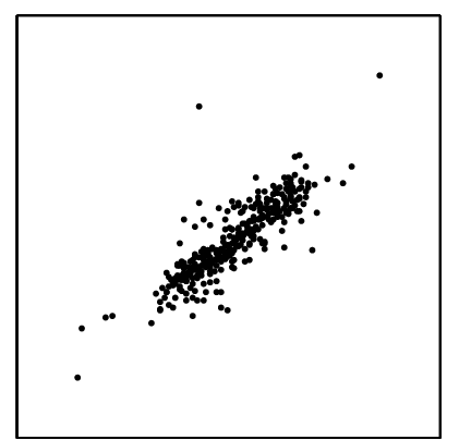
pair0076

Figure 39: Scatter plots of pairs from D24. pair0076: population growth $\rightarrow$ food consumption growth.

pair0076: Population Growth $\rightarrow$ Food Consumption Growth

We regard population growth to cause food consumption growth, mainly because more people eat more. Both variables are most likely also confounded by the availability of food, driven for instance by advances in agriculture and subsequently increasing yields, but also by national and international conflicts, the global food market and other economic factors. However, for the short time period considered here, confounders which mainly influence the variables on a temporal scale can probably be neglected. Their might also be a causal link from food consumption growth to population growth, for instance one could imagine that if people are well fed, they also reproduce more. However, we assume this link only plays a minor role here.

D25: Light response data

The filtered version of the light response data was obtained from Moffat (2012). It consists of 721 measurements of Net Ecosystem Productivity (NEP) and three different measures of the Photosynthetic Photon Flux Density (PPFD): the direct, diffuse, and total PPFD. NEP is a measure of the net $CO_{2}$ flux between the biosphere and the atmosphere, mainly driven by biotic activity. It is defined as the photosynthetic carbon uptake minus the carbon release by respiration, and depends on the available light. NEP is measured in units of $\mu\mathrm{mol\,CO_{2}}\,\mathrm{\,}\mathrm{m}^{-2}\,\mathrm{s}^{-1}$. PPFD measures light intensity in terms of photons that are available for photosynthesis, i.e., with wavelength between 400 nm and 700 nm (visible light). More precisely, PPFD is defined as the number of photons with wavelength of 400–700 nm falling on a certain area per time interval, measured in units of $\mu\mathrm{mol\,photons}\,\mathrm{m}^{-2}\,\mathrm{s}^{-1}$. The total PPFD is the sum of PPFDdif, which measures only diffusive photons, and PPFDdir, which measures only direct (solar light) photons. The data was measured over several hectare of a forest in Hainich, Germany (site name DE-Hai, latitude: $51.08^{\circ}$N, longitude: $10.45^{\circ}$E), and is available from http://fluxnet.ornl.gov.

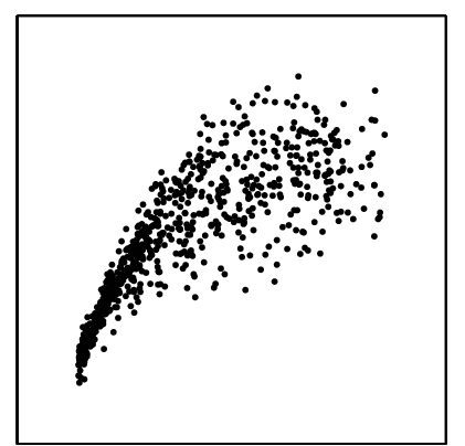
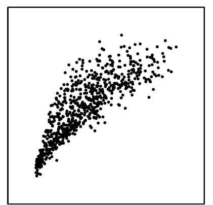
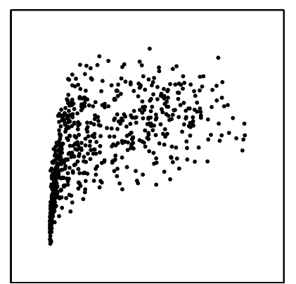
pair0078 pair0079 pair0080

Figure 40: Scatter plots of pairs from D25. pair0078: PPFD $\rightarrow$ NEP, pair0079: PPFDdif $\rightarrow$ NEP, pair0080: PPFDdir $\rightarrow$ NEP.

pair0078–pair0080: {PPFD,PPFDdif,PPFDdir} $\rightarrow$ NEP

Net Ecosystem Productivity is known to be driven by both the direct and the diffuse Photosynthetic Photon Flux Density, and hence also by their sum, the total PPFD.

D26: FLUXNET

The data set contains measurements of net $CO_{2}$ exchanges between atmosphere and biosphere aggregated over night, and the corresponding temperature. It is taken from the FLUXNET network (Baldocchi et al., 2001), available at http://fluxnet.ornl.gov (see also Section D25). The data have been collected at a 10 Hz rate and was aggregated to one value per day over one year (365 values) and at three different sites (BE-Bra, DE-Har, US-PFa). $CO_{2}$ exchange measurements typically have a footprint of about 1km². The data set contains further information on the quality of the data (“1” means that the value is credible, “NaN” means that the data point has been filled in).

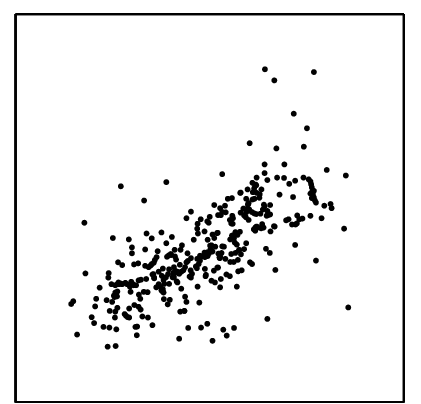
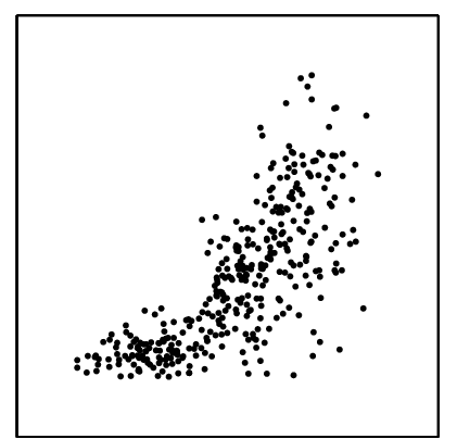
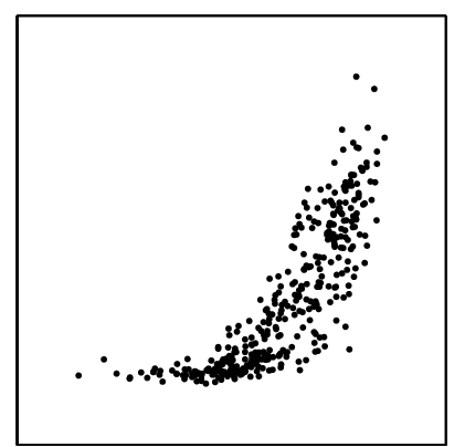
pair0081 pair0082 pair0083

Figure 41: Scatter plots of pairs from D26. pair0081 (BE-Bra): temperature $\rightarrow$ local $CO_{2}$ flux, pair0082 (DE-Har): temperature $\rightarrow$ local $CO_{2}$ flux, pair0083 (US-PFa): temperature $\rightarrow$ local $CO_{2}$ flux.

pair0081–pair0083: Temperature $\rightarrow$ Local $CO_{2}$ Flux

Because of lack of sunlight, $CO_{2}$ exchange at night approximates ecosystem respiration (carbon release from the biosphere to the atmosphere), which is largely dependent on temperature (e.g. Mahecha et al., 2010). The $CO_{2}$ flux is mostly generated by microbial decomposition in soils and maintenance respiration from plants and does not have a direct effect on temperature. We thus consider temperature causing $CO_{2}$ flux as the ground truth. The three pairs pair0081–pair0083 correspond with sites BE-Bra, DE-Har, US-PFa, respectively.

D27: US county-level growth data

The data set (Wheeler, 2003), available at http://www.spatial-econometrics.com/data/contents.html, contains both employment and population information for 3102 counties in the US in 1980. We selected columns eight and nine in the file “countyg.dat”. Column eight contains the natural logarithm of the number of employed people, while column nine contains the natural logarithm of the total number of people living in this county, and is therefore always larger than the number in column eight.

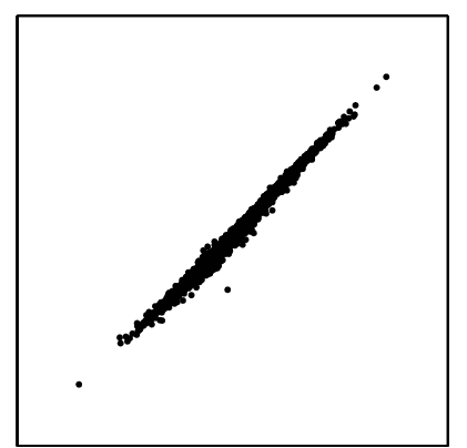
pair0084

Figure 42: Scatter plots of pairs from D27. pair0084: population $\rightarrow$ employment.

pair0084: Population $\rightarrow$ Employment

It seems reasonable that the total population causes the employment and not vice versa. If we increase the number of people living in an area, this has a direct effect on the number of employed people. We believe that the decision to move into an economically strong area is rather based on the employment rate rather than the absolute number of employed people. There might be an effect that the employment status influences the decision to get children but we regard this effect to be less relevant.

D28: Milk protein trial

This data set is extracted from that for the milk protein trial used by Verbyla and Cullis (1990). The original data set consists of assayed protein content of milk samples taken weekly from each of $79$ cows. The cows were randomly allocated to one of three diets: barley, mixed barley-lupins, and lupins, with $25$, $27$ and $27$ cows in the three groups, respectively. Measurements were taken for up to $19$ weeks but there were $38$ drop-outs from week $15$ onwards, corresponding to cows who stopped producing milk before the end of the experiment. We removed the missing values (drop-outs) in the data set: we did not consider the measurements from week 15 onwards, which contain many drop-outs, and we discarded the cows with drop-outs before week 15. Finally, the data set contains 71 cows and 14 weeks, i.e., 994 samples in total. Furthermore, we re-organized the data set to see the relationship between the milk protein and the time to take the measurement. We selected two variables: the time to take weekly measurements (from 1 to 14), and the protein content of the milk produced by each cow at that time.

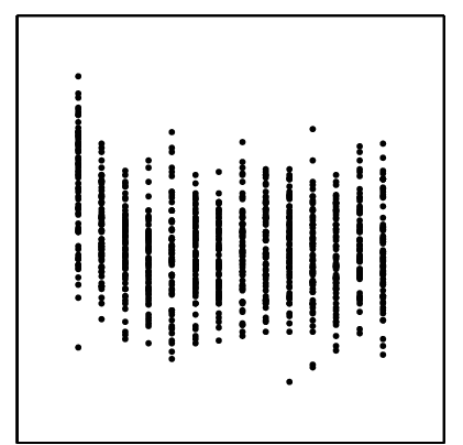
pair0085

Figure 43: Scatter plots of pairs from D28. pair0085: time of measurement $\rightarrow$ protein content of milk.

pair0085: Time of Measurement $\rightarrow$ Protein Content of Milk

Clearly, the time of the measurement causes the protein content and not vice versa. We do not consider the effect of the diets on the protein content.

D29: kamernet.nl data

This data was collected by Joris M. Mooij from http://www.kamernet.nl, a Dutch website for matching supply and demand of rooms and appartments for students, in 2007. The variables of interest are the size of the appartment or room (in $\mathrm{m}^{2}$) and the monthly rent in EUR. Two outliers (one with size $0\,\mathrm{m}^{2}$, the other with rent of 1 EUR per month) were removed, after which 666 samples remained.

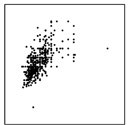
pair0086

Figure 44: Scatter plots of pairs from D29. pair0086: size of apartment $\rightarrow$ monthly rent.

pair0086: Size of apartment $\rightarrow$ Monthly rent

Obviously, the size causes the rent, and not vice versa.

D30: Whistler daily snowfall

The Whistler daily snowfall data is one of the data sets on http://www.mldata.org, and was originally obtained from http://www.climate.weatheroffice.ec.gc.ca/ (Whistler Roundhouse station, identifier 1108906). We downloaded it from http://www.mldata.org/repository/data/viewslug/whistler-daily-snowfall. It concerns historical daily snowfall data in Whistler, BC, Canada, over the period July 1, 1972 to December 31, 2009. It was measured at the top of the Whistler Gondola (Latitude: 50^∘04^′04.000^′′ N, Longitude: 122^∘56^′50.000^′′ W, Elevation: 1835 m). We selected two attributes, mean temperature (^∘C) and total snow (cm). The data consists of 7753 measurements of these two attributes.

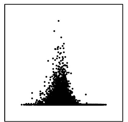
pair0087

Figure 45: Scatter plots of pairs from D30. pair0087: temperature $\rightarrow$ total snow.

pair0087: Temperature $\rightarrow$ Total Snow

Common sense tells us that the mean temperature is one of the causes of the total amount of snow, although there may be a small feedback effect of the amount of snow on temperature. Confounders are expected to be present (e.g., whether there are clouds).

D31: Bone Mineral Density

This dataset comes from the R package ElemStatLearn, and contains measurements of the age and the relative change of the bone mineral density of 261 adolescents. Each value is the difference in the spinal bone mineral density taken on two consecutive visits, divided by the average. The age is the average age over the two visits. We preprocessed the data by taking only the first measurement for each adolescent, as each adolescent has 1–3 measurements.

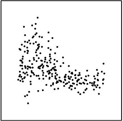
pair0088

Figure 46: Scatter plots of pairs from D31. pair0088: age $\rightarrow$ relative bone mineral density.

pair0088: Age $\rightarrow$ Bone mineral density

Age must be the cause, bone mineral density the effect.

D32: Soil properties

These data were collected within the Biodiversity Exploratories project, see http://www.biodiversity-exploratories.de. We used dataset 14686 (soil texture) and 16666 (root decomposition). With the goal to study fine root decomposition rates, Solly et al. (2014) placed litterbags containing fine roots in 150 forest and 150 grassland sites along a climate gradient across Germany. Besides the decomposition rates, a range of other relevant variables were measured, including soil properties such as clay content, soil organic carbon content and soil moisture. We deleted sites with missing values and separated grasslands and forests.

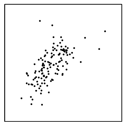
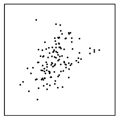
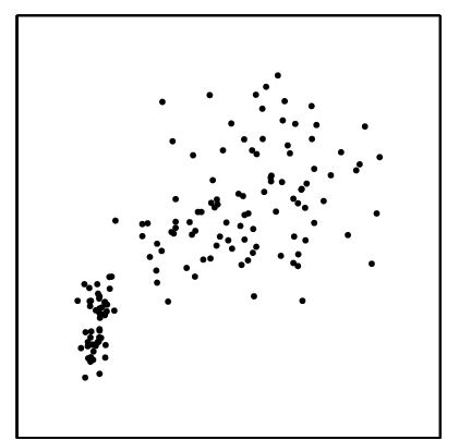
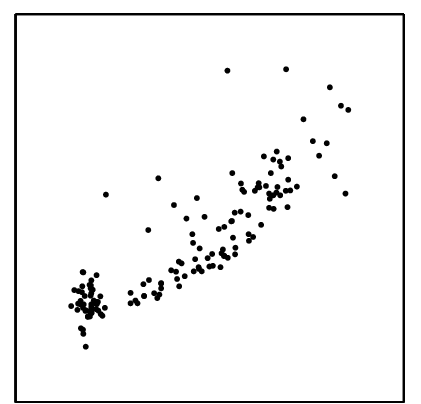
pair0089 pair0090 pair0091 pair0092

Figure 47: Scatter plots of pairs from D32. pair0089: Root decomposition in April $\rightarrow$ Root decomposition in October (Forests), pair0090: Root decomposition in April $\rightarrow$ Root decomposition in October (Grasslands), pair0091: Clay content in soil $\rightarrow$ Soil moisture (forests), pair0092: Clay content in soil $\rightarrow$ Organic carbon content (forests).

pair0089–pair0090: Root decomposition in April $\rightarrow$ Root decomposition in October

Root decomposition happens monotonously in time. Hence the amount decomposed in April directly affects the amount decomposed in October in the same year.

pair0091: Clay content in soil $\rightarrow$ Soil moisture

The amount of water that can be stored in soils depends on its texture. The clay content of a soil influences whether precipitation is stored longer in soils or runs off immediately. In contrast, it is clear that wetness of a soil does not affect its clay content.

pair0092: Clay content in soil $\rightarrow$ Organic carbon content

How much carbon an ecosystem stores in its soil depends on multiple factors, including the land cover type, climate and soil texture. Higher amounts of clay are favorable for storage of organic carbon (Solly et al., 2014). Soil organic carbon, on the other hand, does not alter the texture of a soil.

D33: Runoff data

This dataset comes from the MOPEX data base (http://www.nws.noaa.gov/ohd/mopex/mo_datasets.htm and can be downloaded directly from ftp://hydrology.nws.noaa.gov/pub/gcip/mopex/US_Data/Us_438_Daily/. It contains precipitation and runoff data from over 400 river catchments in the USA on a daily resolution from 1948 to 2004. We computed yearly averages of precipitation and runoff for each catchment.

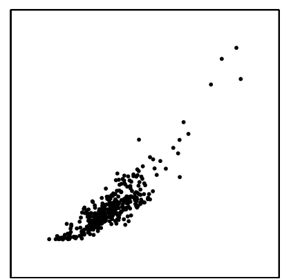
pair0093

Figure 48: Scatter plots of pairs from D33. pair0093: Precipitation $\rightarrow$ Runoff.

pair0093: Precipitation $\rightarrow$ Runoff

Precipitation is by far the largest driver for runoff in a given river catchment. There might be a very small feedback from runoff that evaporates and generates new precipitation. This is, however, negligible if the catchment does not span over full continents.

D34: Electricity load

This data set comes from a regional energy distributor in Turkey. It contains three variables, the hour of the day, temperature in degree Celsius and electricity consumption (load) in MW per hour. We are thank S. Armagan Tarim and Steve Prestwich for providing the data.

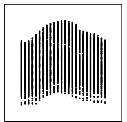
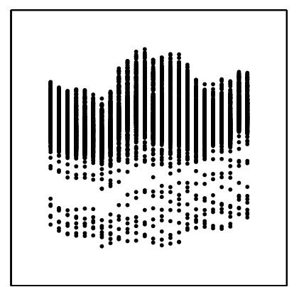
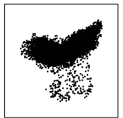
pair0094 pair0095 pair0096

Figure 49: Scatter plots of pairs from D34. pair0094: Hour of the day $\rightarrow$ Temperature, pair0095: Hour of the day $\rightarrow$ Electricity consumption, pair0096: Temperature $\rightarrow$ Electricity consumption.

pair0094: Hour of the day $\rightarrow$ Temperature

We consider hour of the day as the cause, since it can be seen as expressing the angular position of the sun. Although true interventions are unfeasible, it is commonly agreed that changing the position of the sun would result in temperature changes at a fixed location due to the different solar incidence angle.

pair0095: Hour of the day $\rightarrow$ Electricity consumption

The hour of the day constrains in many ways what people do and thus also their use of electricity. Consequently, we consider hour of the day as cause and electricity consumption as effect.

pair0096: Temperature $\rightarrow$ Electricity consumption

Changes in temperature can prompt people to use certain electric devices, e.g., an electric heating when it is gets very cold or the usage of a fan or air conditioning when it gets very hot. Furthermore, certain machines such as computers have to be cooled more if temperatures rise. Hence we consider temperature as cause and electricity consumption as effect.

D35: Ball track

The data has been recorded by D. Janzing using a ball track that has been equipped with two pairs of light barriers. The first pair measures the initial speed and the second pair the speed of a ball at some later position of the track. The units are arbitrary and differ for both measurements since they are obtained by inverting the time the ball needed to pass the distance between two light barriers of one pair.

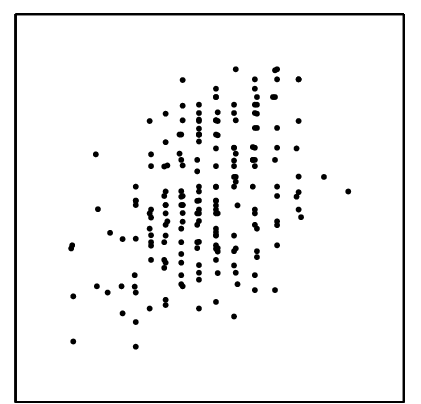
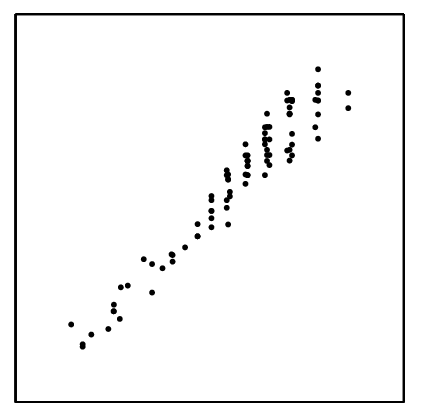
pair0097 pair0098

Figure 50: Scatter plots of pairs from D35. pair0097: Initial speed $\rightarrow$ Final speed, pair0098: Initial speed $\rightarrow$ Final speed.

The initial part of the track has large slope. The initial speed is strongly determined by the exact position where the ball is put on the track. For part of the runs, the position of the ball has been chosen by D. Janzing, the other part by a 4-year old child. This should avoid that the variation of the initial position is done in a too systematic way.

Two similar experiments have been performed, using different ball track setups. For pair0098 the ball track had a longer acceleration zone than for pair0097, which allows for larger variations in initial speed.

pair0097: Initial speed $\rightarrow$ Final speed

These data consists of 202 measurements. Obviously, the initial speed of the ball causes the final speed.

pair0098: Initial speed $\rightarrow$ Final speed

These data consist of 94 measurements. Again, the initial speed of the ball causes the final speed.

D36: nlschools

This is dataset nlschools from the R package MASS. The data were used by Snijders and Bosker (1999) as a running example and are about a study of 2287 eigth-grade pupils (aged about 11) in 132 classes in 131 schools in the Netherlands. We used two variables: lang, a language test score, and SES, the social-economic status of the pupil’s family.

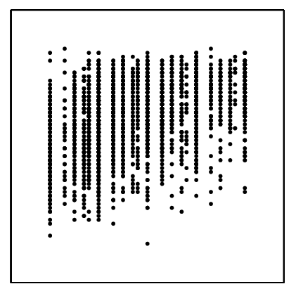
pair0099

Figure 51: Scatter plots of pairs from D36. pair0099: Social-economic status of family $\rightarrow$ Language test score.

pair0099: Social-economic status of family $\rightarrow$ Language test score

We consider the social-economic status of the pupil’s family to be the cause of the language test score of the pupil. However, note that selection bias may be present via the choice of the schools to include in the study.

D37: cpus

This is dataset cpus from the R package MASS, and concerns characteristics of 209 CPUs (Ein-Dor and Feldmesser, 1987). We used two variables: syct, cycle time in nanoseconds, and perf, the published performance on a benchmark mix relative to an IBM 370/158-3, and took the logarithms of the original values.

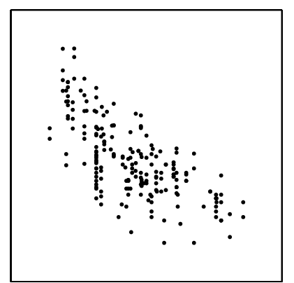
pair0100

Figure 52: Scatter plots of pairs from D37. pair0100: CPU cycle time $\rightarrow$ Performance.

pair0100: CPU cycle time $\rightarrow$ Performance

It should be obvious that CPU cycle time causes its performance.

E Computation time

We report the total computation time for each benchmark set and for each of our implementations of various methods in Figures 53 and 54. We used a machine with Intel Xeon CPU E5-2680 v2 @ 2.80GHz processors, 40 cores, and 125 GB of RAM. The measured computation time measures the total time spent (i.e., the sum of the computation times of individual cores). We did not spend much effort on optimizing the implementations, so the reported computation times should be seen as upper bounds on what is achievable. We only report results for the unperturbed data, as the preprocessing does not affect computation time significantly.

In general, for the ANM implementations, most time is taken by the Gaussian Process regression. The HSIC test and entropy estimators are relatively quick compared to that. A notable outlier is ANM-MML which spends much time on estimating the MML of the marginal distribution using the algorithm by Figueiredo and Jain (2002). IGCI implementations are much faster than ANM (about two orders of magnitude in our setting), as non-parametric regression is not required. One notable outlier for the IGCI implementations is IGCI-ent-PSD, which shows that the ent-PSD estimator is slower than the other entropy estimators in the ITE toolbox. Interestingly, this is also the only non-parameteric entropy estimator that turned out to be robust to perturbations of the data.

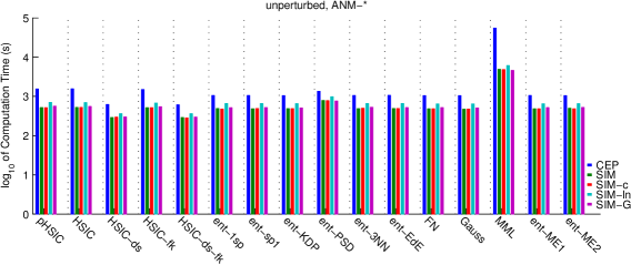
Figure 53: Computation times of various ANM methods on different (unperturbed) data sets. For the variants of the spacing estimator, only the results for sp1 are shown, as results for sp2,…,sp6 were similar.

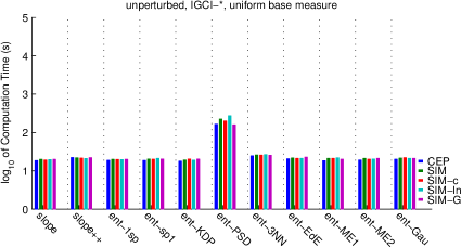
Figure 54: Computation times of various IGCI methods on different (unperturbed) data sets. For the variants of the spacing estimator, only the results for sp1 are shown, as results for sp2,…,sp6 were similar. We only show results for the uniform base measure as those for the Gaussian base measure are similar.

References

- Armann and Bülthoff (2012) R. Armann and I. Bülthoff. Male and female faces are only perceived categorically when linked to familiar identities – and when in doubt, he is a male. Vision Research, 63:69–80, 2012.
- Azzalini and Bowman (1990) A. Azzalini and A. W. Bowman. A look at some data on the Old Faithful Geyser. Applied Statistics, 39(3):357–365, 1990.
- Bache and Lichman (2013) K. Bache and M. Lichman. UCI Machine Learning Repository, 2013. URL http://archive.ics.uci.edu/ml.
- Baldocchi et al. (2001) D. Baldocchi, E. Falge, L. Gu, R. Olson, D. Hollinger, S. Running, P. Anthoni, C. Bernhofer, K. Davis, R. Evans, J. Fuentes, A. Goldstein, G. Katul, B. Law, X. Lee, Y. Malhi, T. Meyers, W. Munger, W. Oechel, K. T. Paw, K. Pelegaard, H. P. Schmid, R. Valentini, S. Verma, T. Vesala, K. Wilson, and S. Wofsy. FLUXNET: A new tool to study the temporal and spatial variability of ecosystem-scale carbon dioxide, water vapor, and energy flux densities. Bulletin of the American Meteorological Society, 82(11):2415–2434, 2001.
- Baynes and Dominiczak (1999) J. Baynes and M. H. Dominiczak. Medical Biochemistry. Mosby, 1999.
- Bloomer et al. (2009) J. Bloomer, J. W. Stehr, C. A. Piety, R. J. Salawitch, and R. R. Dickerson. Observed relationships of ozone air pollution with temperature and emissions. Geophysical Letters, 36(9), 2009.
- Bollen (1989) K. A. Bollen. Structural Equations with Latent Variables. John Wiley & Sons, 1989.
- Braunwald et al. (2001) E. Braunwald, A. S. Fauci, D. L. Kasper, S. L. Hauser, D. L. Long, and J. L. Jameson, editors. Principles of Internal Medicine: Volume 2. McGraw-Hill, 15th international edition, 2001.
- Bühlmann et al. (2014) P. Bühlmann, J. Peters, and J. Ernest. CAM: Causal additive models, high-dimensional order search and penalized regression. Annals of Statistics (to appear), ArXiv e-prints (1207.5136), 2014.
- Clopper and Pearson (1934) C. Clopper and E. S. Pearson. The use of confidence or fiducial limits illustrated in the case of the binomial. Biometrika, 26:404–413, 1934.
- Cover and Thomas (2006) T. M. Cover and J. A. Thomas. Elements of Information Theory. Wiley-Interscience, 2006.
- Czerniak and Zarzycki (2003) J. Czerniak and H. Zarzycki. Application of rough sets in the presumptive diagnosis of urinary system diseases. In J. Soldek and L. Drobiazgiewicz, editors, Artificial Intelligence and Security in Computing Systems, pages 41–51. Kluwer Academic Publishers, Norwell, MA, USA, 2003.
- Daniušis et al. (2010) P. Daniušis, D. Janzing, J. M. Mooij, J. Zscheischler, B. Steudel, K. Zhang, and B. Schölkopf. Inferring deterministic causal relations. In Proceedings of the 26th Annual Conference on Uncertainty in Artificial Intelligence (UAI 2010), pages 143–150, 2010.
- Eaton and Murphy (2007) D. Eaton and K. Murphy. Exact Bayesian structure learning from uncertain interventions. In Proceedings of the 11th International Conference on Artificial Intelligence and Statistics (AISTATS), pages 107–114, 2007.
- Eberhardt and Scheines (2007) F. Eberhardt and R. Scheines. Interventions and causal inference. Philosophy of Science, 74(5):981–995, 2007.
- Ebrahimi et al. (1994) N. Ebrahimi, K. Pflughoeft, and E. S. Soofi. Two measures of sample entropy. Statistics and Probability Letters, 20:225–234, 1994.
- Ein-Dor and Feldmesser (1987) P. Ein-Dor and J. Feldmesser. Attributes of the performance of central processing units: a relative performance prediction model. Communications of the ACM, 30:308–317, 1987.
- Esrey et al. (1991) S. A. Esrey, J. B. Potash, L. Roberts, and C. Shiff. Effects of improved water supply and sanitation on ascariasis, diarrhoea, dracunculiasis, hookworm infection, schistosomiasis, and trachoma. Bulletin of the World Health Organization, 69(5):609, 1991.
- Feister and Balzer (1991) U. Feister and K. Balzer. Surface ozone and meteorological predictors on a subregional scale. Atmospheric Environment. Part A. General Topics, 25(9):1781–1790, 1991.
- Figueiredo and Jain (2002) M. A. T. Figueiredo and A. K. Jain. Unsupervised learning of finite mixture models. IEEE Transactions on Pattern Analysis and Machine Intelligence, 24(3):381–396, March 2002.
- Friedman and Nachman (2000) N. Friedman and I. Nachman. Gaussian process networks. In Proceedings of the 16th Annual Conference on Uncertainty in Artificial Intelligence (UAI 2000), pages 211–219, 2000.
- Fukumizu et al. (2008) K. Fukumizu, A. Gretton, X. Sun, and B. Schölkopf. Kernel measures of conditional dependence. In Advances in Neural Information Processing Systems 20 (NIPS*2007), pages 489–496, 2008.
- Gray (2006) R. M. Gray. Toeplitz and circulant matrices: A review. Foundations and Trends in Communications and Information Theory, 2:155–239, 2006.